LICORS: Light Cone Reconstruction of States for Non-parametric Forecasting of Spatio-Temporal Systems

Abstract

We present a new, non-parametric forecasting method for data where continuous values are observed discretely in space and time. Our method, light-cone reconstruction of states (LICORS), uses physical principles to identify predictive states which are local properties of the system, both in space and time. LICORS discovers the number of predictive states and their predictive distributions automatically, and consistently, under mild assumptions on the data source. We provide an algorithm to implement our method, along with a cross-validation scheme to pick control settings. Simulations show that CV-tuned LICORS outperforms standard methods in forecasting challenging spatio-temporal dynamics. Our work provides applied researchers with a new, highly automatic method to analyze and forecast spatio-temporal data.

Keywords: non-parametric prediction, dynamical system, forecasting, predictive state reconstruction, spatio-temporal data.

1 Introduction

Many important scientific and data-analytic problems involve fields which vary over both space and time, e.g., data from functional magnetic resonance imaging, meteorological observations, or experimental studies in physics and chemistry. An outstanding objective in studying such data is prediction, where we want to describe the field in the future.

Spatio-temporal data being increasingly easy to acquire, manipulate and visualize, statisticians have developed corresponding methods for statistical inference, reviewed in works like Finkenstadt-Held-Isham-spatio-temporal-systems,Cressie-Wikle-spatio-temporal-data. The usual tools are a combination of ways of describing the distribution of the random field (e.g., various dependency measures), and stochastic modeling, focusing primarily on parametric inference, and secondarily on parameter-conditional predictions.

While these approaches are valuable, there is a complementary role for direct, non-parametric prediction of spatio-temporal data, just as with time series Bosq-nonparametric,Fan-Yao-time-series. Our aim here is to blend modern methods of non-parametric prediction with insights from nonlinear physics on the organization of spatial dynamics, yielding predictors of spatio-temporal evolution that are computationally efficient and make minimal assumptions on the data source, but are still accurate and even interpretable.

The idea behind our approach is simply that it takes time for influences to propagate across space, so we can constrain the search for predictors to a spatio-temporally local neighborhood at each point. We combine this with a novel form of non-parametric smoothing, which infers the prediction (regression or conditional probability) function by averaging together similar observations, where “similarity” is defined in terms of predictive consequences, effectively replacing the original geometry of the predictor variables with a new one, optimized for forecasting. The combination of these two tools lets us discover underlying structures, as well make fast and accurate predictions.

Section 2 formally defines our prediction problem and introduces our non-parametric localized approach. Section 3 gives the statistical methods to estimate these optimal predictors from discretely-observed continuous-valued fields. Section 4 shows, under weak conditions on the data-generating process, that our method consistently estimates the predictive distributions. Section 5 proposes a cross-validation scheme to choose our control settings, and compares our predictive accuracy to standard time series techniques. Finally, Section 6 summarizes this new methodology and discusses future work. Proofs and implementation details can be found in the Supplementary Material.

2 Local Prediction of Spatio-temporal Fields

2.1 Setting and Notation; Light Cones

We observe a random field $(X\left(\mathbf{r},t\right))_{\mathbf{r}\in\mathbf{S},t\in\mathbb{T}}$ in discrete space and time. The field takes values in a set $\mathcal{X}$, which may be discrete or continuous. Space $\mathbf{S}$ is a regular lattice, equipped with norm $\lVert\mathbf{r}\rVert$. Time $\mathbb{T}$ is taken to be the positive integers up to $T$.

Suppose that disturbances or influences in the system have a maximum speed of propagation, $c$. Then the only events which could affect what happens at a given $\left(\mathbf{r},t\right)$ are those where $s\leq t$ and $\lVert\mathbf{r}-\mathbf{u}\rVert\leq c(t-s)$. Since this set grows as $s$ recedes into the past, we call this the past light cone (PLC) of $\left(\mathbf{r},t\right)$. The future light cone (FLC) are all events which could be affected by the present moment $\left(\mathbf{r},t\right)$; it thus consists of all those $\left(\mathbf{u},s\right)$, where $s>t$ and $\lVert\mathbf{r}-\mathbf{u}\rVert\leq c(s-t)$. Light cones look like triangles in $(1+1)D$ fields, and in $(2+1)D$, pyramids (Fig. 1). Denote the configuration in the past cone of $\left(\mathbf{r},t\right)$ by $L^{-}\left(\mathbf{r},t\right)$:

$$L^{-}\left(\mathbf{r},t\right)=\left\{X\left(\mathbf{u},s\right)\mid s\leq t,\lVert\mathbf{r}-\mathbf{u}\rVert\leq c(t-s)\right\}$$ (1)

$L^{+}\left(\mathbf{r},t\right)$ is, similarly, the configuration in the future cone.

The spatio-temporal prediction problem is thus: use the configuration of the past cone, $L^{-}\left(\mathbf{r},t\right)$, to forecast the configuration of the future cone, $L^{+}\left(\mathbf{r},t\right)$. Light-cone prediction compromises between capturing global patterns and needing only local information. We will construct optimal predictors for light cones presently. Light cones can be defined for spatial extended patches of points. (When the “patch” becomes the whole spatial lattice, we are back to global prediction.) This leads to a parallel theory of prediction, but it turns out that the predictive state of a patch is determined by the predictive states of its points [§3.3, Lemma 2 and Theorem 3]CRS-prediction-on-networks, so we lose no information, and gain tractability, by not considering cones for patches.

(a)

(b)

Figure 1: Past (red) and future (blue) light cones in a $(1+1)D$ (a) and $(2+1)D$ (b) system. Here $c$, the velocity of signal propagation, is set to $1$. The past cone is truncated at a horizon of $h_{p}=3$ steps, while the future cone’s horizon is only $h_{f}=2$. Whether the present (green) is included in the past or the future cone is a matter of convention; see Section 5.

Computationally, we need to truncate the cones at a finite number of time steps — we will call these the past horizon $h_{p}$ of $L^{-}$, and likewise the future horizon $h_{f}$ of $L^{+}$. Doing this reduces $L^{+}$ and $L^{-}$ to finite-dimensional random vectors. (For instance, in Fig. 1, with $h_{p}=3$ and $c=1$, $\ell^{-}\left(\mathbf{r},t\right)$ has 15 degrees of freedom.) The horizons are control settings, and may be tuned through (for example) cross-validation (§5.2). Similarly, when the maximum speed of propagation $c$ is not given from background knowledge, it is also a control setting.

2.2 Predictive States

To predict the future $L^{+}\left(\mathbf{r},t\right)$ from a particular past configuration, say $\ell^{-}$, requires knowing the conditional distribution

$$\mathbb{P}\left(L^{+}\left(\mathbf{r},t\right)\mid L^{-}\left(\mathbf{r},t\right)=\ell^{-}\right)$$ (2)

for all $\ell^{-}$. (Subsequently $\left(\mathbf{r},t\right)$ may be omitted for readability.) Since treating this conditional distribution as an arbitrary function of $\ell^{-}$ is not feasible statistically or computationally, we try to find a sufficient statistic $\eta$ of past configurations that keeps the predictive information:

$$\mathbb{P}\left(L^{+}\left(\mathbf{r},t\right)\mid H\left(\mathbf{r},t\right)=\eta(\ell^{-})\right)=\mathbb{P}\left(L^{+}\left(\mathbf{r},t\right)\mid L^{-}\left(\mathbf{r},t\right)=\ell^{-}\right)~{}.$$ (3)

There are usually many sufficient statistics $\eta,\eta^{\prime},\ldots$. When $\eta$ and $\eta^{\prime}$ are both sufficient, but $\eta(\ell^{-})=f(\eta^{\prime}(\ell^{-}))$ for some $f$, then $\eta$ is a smaller, more compressed, summary of the data than $\eta^{\prime}$, and so the former is preferred by Occam’s Razor. The minimal sufficient statistic $\epsilon$ compresses the data as much as can be done without losing any predictive power, retaining only what is needed for optimal predictions.

We now construct the minimal sufficient statistic, following CRS-prediction-on-networks, to which we refer for some mathematical details.

Definition 2.1 (Equivalent configurations).

The past configurations $\ell_{i}^{-}$ at $\left(\mathbf{r},t\right)$ and $\ell_{j}^{-}$ at $\left(\mathbf{u},s\right)$ are predictively equivalent, $(\ell_{i}^{-},\left(\mathbf{r},t\right))\sim(\ell_{j}^{-},u\left(\mathbf{s},)\right)$, if they predict the same future with equal probabilities, i.e. if

$$\mathbb{P}\left(L^{+}\left(\mathbf{r},t\right)\mid L^{-}\left(\mathbf{r},t\right)=\ell_{i}^{-}\right)=\mathbb{P}\left(L^{+}\left(\mathbf{u},s\right)\mid L^{-}\left(\mathbf{u},s\right)=\ell_{j}^{-}\right)$$ (4)

Let $\left[(\ell^{-},\left(\mathbf{r},t\right))\right]$ be the equivalence class of $(\ell^{-},\left(\mathbf{r},t\right))$, i.e., the set of all past configurations and coordinates that predict the same future as $\ell^{-}$ does at $\left(\mathbf{r},t\right)$. Let

$$\epsilon(\ell^{-},\left(\mathbf{r},t\right))\equiv\left[\ell^{-}\right]$$ (5)

be the function mapping each $(\ell^{-},\left(\mathbf{r},t\right))$ to its predictive equivalence class. The values $\epsilon$ can take are the predictive states; they are the minimal statistics which are sufficient for predicting $L^{+}$ from $L^{-}$ CRS-prediction-on-networks.

Since each predictive state has a unique predictive distribution and vice versa. We will thus slightly abuse notation to denote by $\mathcal{E}$ both the set of equivalence classes and the set of predictive distributions, whose elements we will write $\epsilon_{j}$. We will further abuse notation by writing the mapping from past cone configurations to predictive distributions as $\epsilon(\cdot)$, leading to the measure-valued random field

$$S\left(\mathbf{r},t\right):=\epsilon\left(L^{-}\left(\mathbf{r},t\right)\right)~{}.$$ (6)

One can show CRS-prediction-on-networks that $S\left(\mathbf{r},t\right)$ is Markov even if $X\left(\mathbf{r},t\right)$ is not. However, $X$ is not an ordinary hidden Markov random field, since there is an unusual deterministic dependence between transitions in $S$ and the realization of $X$, analogous to that of a chain with complete connections Fernandez-Maillard-chains-with-complete-connections.

To be able to draw useful inferences from a single realization of the process, we must assume some form of homogeneity or invariance of the conditional distributions.

Assumption 2.2 (Conditional invariance).

The predictive distribution of a PLC configuration $\ell^{-}$ does not change over time or space. That is, for all $\mathbf{r},t$, all $\mathbf{u},s$, and all past light-cone configurations $\ell^{-}$,

$$(\ell^{-},\left(\mathbf{r},t\right))\sim(\ell^{-},\left(\mathbf{u},s\right))$$ (7)

We may thus regard $\sim$ as an equivalence relation among PLC configurations, and $\epsilon$ as a function over $\ell^{-}$ alone.

This is just conditional invariance, like the conditional stationarity for time series used in Caires-Ferreira-prediction-of-cond-stat-seq. It would be implied by the field being a Markov random field with homogeneous transitions, or of course by full stationarity and spatial invariance, but it is weaker. Assumption 7 lets us talk about the predictive distribution of a PLC configuration, regardless of when or where it was observed, and to draw inferences by pooling such observations. If this assumption fails, we could in principle still learn a different set of predictive states for each moment of time and/or each point of space (as in CRS-prediction-on-networks), but this would need data from multiple realizations of the same process.

3 Estimating Predictive States

We extend the work of CRS-prediction-on-networks,QSO-in-PRL to continuous-valued fields, introducing statistical methods to estimate and predict non-linear dynamics accurately and efficiently, while still obtaining insight into the spatio-temporal structure. Algorithmic details are given in the Supplementary Material.

Assume we have $T$ consecutive measurements of the field $X\left(\mathbf{r},t\right)$, observed over the lattice $\mathbf{S}$, with $N=|\mathbf{S}|\cdot T$ space-time coordinates $\left(\mathbf{r},t\right)$ in all. Each one of these $N$ point-instants has a past and a future light-cone configuration, $\ell^{-}\left(\mathbf{r},t\right)$ and $\ell^{+}\left(\mathbf{r},t\right)$, represented as, respectively, $n_{p}$ and $n_{f}$ dimensional vectors. Since predictive states are sets of PLC configurations with the same predictive distribution, we need to test this sameness, based on conditional samples $\{\ell^{+}\mid\ell_{i}^{-}\}_{i=1}^{N}$ from the observed field. We will apply non-parametric two-sample tests for $H_{0}~{}:~{}\mathbb{P}\left(L^{+}\mid L^{-}=\ell_{i}^{j}\right)=\mathbb{P}\left(L^{+}\mid L^{-}=\ell_{i}^{-}\right)$ pairwise for all $i$ and $j$. Because there are typically a great many past light cones (one for each point-instant), and light-cone configurations are themselves high-dimensional objects, we generally must do this step-wise.

3.1 Partitioning PLC Configurations: Similar Pasts Have Similar Futures

It is often reasonable to assume that the mapping from the past to predictive distributions is regular, so that if two historical configurations are close (in some suitable metric), then their predictive distributions are also close. This lets us avoid having to do some pairwise tests, as their results can be deduced from others.

Assumption 3.1 (Continuous histories).

For every $\rho>0$, there exists a $\delta>0$ such that

$$\lVert\ell_{i}^{-}-\ell_{j}^{-}\rVert<\delta\Rightarrow\mathcal{D}_{KL}\left(\mathbb{P}\left(L^{+}\mid\ell_{i}^{-}\right)\mid\mid\mathbb{P}\left(L^{+}\mid\ell_{j}^{-}\right)\right)<\rho,$$ (8)

where $\mathcal{D}_{KL}\left(p\mid\mid q\right)$ is the Kullback-Leibler divergence between distributions $p$ and $q$ Kullback-info-theory-and-stats.

Assumption 3.1 requires that sufficiently small changes ($<\delta$) in the local past make only negligible ($<\rho$) changes to the distribution of local future outcomes. Statistically, such smoothness-in-distribution lets us pool observations from highly similar PLC configurations, enhancing efficiency; physically, it reflects the smoothness of reasonable dynamical mechanisms. Chaotic systems, where the exact trajectory depends sensitively on initial conditions, do not present difficulties, since Assumption 3.1 is about the conditional distribution of the future given partial information on the past, and chaos has long been recognized as a way to stabilize such distributions, forming the basis for prediction and control of chaos Kantz-Schreiber-2nd.

We use Assumption 3.1 to justify an initial “pre-clustering” of the PLC configuration space, greatly reducing computational cost with little damage to predictions. We first divide the PLC configuration space using fast clustering algorithms into $K\ll N$ clusters, and then test equality of distributions between clusters ($\mathcal{O}(K^{2})$), rather than light cones ($\mathcal{O}(N^{2})$).

When $N$ is small enough, we can skip this initial pre-clustering. To simplify exposition, we treat this as assigning each distinct past cone to its own cluster.

3.2 Partitioning Clusters into Predictive States

Each cluster $P_{k}$ contains a set of similar PLC configurations, and also defines a sample of conditional FLCs, $\mathbf{F}_{k}(\delta)=\{\ell^{+}_{j}\mid\ell^{-}_{j}\in P_{k}\}\in\mathbb{R}^{N_{k}\times n_{f}}$, $k=1,\ldots,K$. Since all $\ell_{j}^{-}\in P_{k}$ have very similar distribution, $\mathbf{F}_{k}\sim Q$ is an approximate sample from the predictive distribution $\mathbb{P}\left(L^{+}\left(\mathbf{r},t\right)\mid\ell^{-}\in P_{k}\right)$. Lemma 4.7, below, shows that for sufficiently small $\delta$, $\mathbf{F}_{k_{i}}(\delta)$ is an exact sample of $p(\epsilon(P_{k_{i}}))$. Thus, to simplify the exposition, we ignore the $\rho$ difference in this section.

Thus, finding equivalent clusters reduces to testing hypotheses of the form $H_{0}:p_{k_{i}}=p_{k_{j}}$ based on the two samples $\mathbf{F}_{k_{i}}(\delta)$ and $\mathbf{F}_{k_{j}}(\delta)$. For $h_{f}=0$ and $c=1$, FLCs are one-dimensional and we can use a Kolmogorov-Smirnov test (or any other two-sample univariate test). In general, however, $\mathbf{F}_{k}$ are samples from a very high-dimensional distribution, and we use non-parametric, multivariate, two-sample tests [see e.g.][]Rosenbaum05_ExactTwosampleTest, RizzoSzekely10_DISCO,Grettonetal07_twosample_kernel. Any test satisfying Assumption 4.11 could be used.

To estimate the predictive states from an initial partitioning of PLC configurations, we iterate through the list of configurations, recursively testing equality of distributions. To initialize the algorithm, create the first predictive state $\epsilon_{1}$, containing the first configuration $\ell_{1}^{-}$. Then take $\ell^{-}_{2}$ and test if its distribution is equal to that of $\epsilon_{1}$. If it is (at the level $\alpha$), then put $\ell_{2}^{-}$ in $\epsilon_{1}$; otherwise generate a new predictive state $\epsilon_{2}$ with $\ell_{2}^{-}$. Then test the next configuration against all previously established predictive states and proceed as before. This continues until all configurations have been assigned to a predictive state.

The predictive distribution of each predictive state can be found by applying any consistent non-parametric density estimator to the future cone samples belonging to that state. If we only want point forecasts, we can skip estimating the whole predictive distribution and just get (e.g.) the mean of the samples.

4 Consistency

LICORS consistently recovers the correct assignment of past cone configurations to predictive states, and the predictive distributions, under weak assumptions on the data-generating process. These allow for the number of predictive states to grow slowly with the sample size, so that we have non-parametric consistency. We give all assumptions and lemmas in the main text; proofs are in the Supplementary Material.

4.1 Assumptions

Let $N=|\mathbf{S}\times\mathbb{T}|$ be the total number of space-time points at which we observe both the past and future light cone. We presume that $N\rightarrow\infty$, without caring whether $|\mathbf{S}|\rightarrow\infty$, $|\mathbb{T}|\rightarrow\infty$, or both.

Assumption 4.1 (Slowly growing number of predictive states).

The number of predictive states, $|\mathcal{E}|=m(N)=\operatorname{o}\bigl{(}N\bigr{)}$, and always $\leq N$.

Assumption 4.1 only guarantees that at least one of the predictive states grows in size. To bound testing error probabilities, the number of light cones seen in every state must grow as $N$ grows.

Assumption 4.2 (Increasing number of light cones in each state).

The number of light cones in each state, $N_{j}:=|\epsilon_{j}|$, grows with $N$: for all $\epsilon_{j}\in\mathcal{E}$,

$$\lim_{N\rightarrow\infty}{N_{j}(N)}=\infty$$ (9)

Let $N_{\min}=\min_{j}N_{j}$ be the number of samples in the smallest predictive state; thus also $N_{\min}\rightarrow\infty$ for $N\rightarrow\infty$. Assumption 4.2 means that the system re-visits each predictive state as it evolves, i.e., all states are recurrent. This lets us learn the predictive distribution of each state, from a growing sample of its behavior.

Assumption 4.3 (Bounded conditional distributions).

All predictive distributions $\epsilon_{j}\in\mathcal{E}$ have densities with respect to a common reference measure $\nu$, and $0<\iota<d\epsilon_{j}/d\nu<\kappa<\infty$, for some constants $\iota$ and $\kappa$.

This merely technical assumption guarantees bounded likelihood ratios.

Assumption 4.4 (Distinguishable predictive states).

The KL divergence between states is bounded from below: $\forall i\neq j$,

$$0<d_{\min}\leq\mathcal{D}_{KL}\left(\epsilon_{i}\mid\mid\epsilon_{j}\right)=:d_{i,j}$$ (10)

We do not need $d_{i,j}<\infty$. (In fact, $\mathcal{D}_{KL}\left(\epsilon_{i}\mid\mid\epsilon_{j}\right)=\infty$ is helpful.) (10) is automatically satisfied for any fixed number of states. For an increasing state space, $m=m(N)$, assume

$$\inf_{i,j\in m(N)}d_{i,j}=d_{\min}>0\text{ for }N\rightarrow\infty.$$ (11)

Lemma 4.5 (Conditionally independent FLCs).

If the cones $L^{+}\left(\mathbf{r},t\right)$ and $L^{+}\left(\mathbf{u},s\right)$ do not overlap, then

$$L^{+}\left(\mathbf{r},t\right)\mathchoice{\mathrel{\hbox{$\displaystyle\perp$}\kern-10.27771pt\mkern 4.0mu\hbox{$\displaystyle\perp$}}}{\mathrel{\hbox{$\textstyle\perp$}\kern-10.27771pt\mkern 4.0mu\hbox{$\textstyle\perp$}}}{\mathrel{\hbox{$\scriptstyle\perp$}\kern-8.02771pt\mkern 4.0mu\hbox{$\scriptstyle\perp$}}}{\mathrel{\hbox{$\scriptscriptstyle\perp$}\kern-6.52771pt\mkern 4.0mu\hbox{$\scriptscriptstyle\perp$}}}L^{+}\left(\mathbf{u},s\right)\mid S\left(\mathbf{r},t\right),S\left(\mathbf{u},s\right).$$ (12)

In particular,

$$\mathbb{P}\left(L^{+}\left(\mathbf{r},t\right),L^{+}\left(\mathbf{u},s\right)\mid S\left(\mathbf{r},t\right),S\left(\mathbf{u},s\right)\right)=\mathbb{P}\left(L^{+}\left(\mathbf{r},t\right)\mid S\left(\mathbf{r},t\right)\right)\mathbb{P}\left(L^{+}\left(\mathbf{u},s\right)\mid S\left(\mathbf{u},s\right)\right)~{}.$$ (13)

Corollary 4.6.

If $h_{f}=0$, then FLCs are conditionally independent given their predictive state.

4.1.1 Getting samples from $\epsilon_{i}$

We get a sample of FLCs from the predictive distribution of $\ell_{i}$ by first taking all PLCs in a $\delta$-neighborhood around $\ell_{i}$,

$$I_{i}(\delta)=\{j\mid\lVert\ell_{i}^{-}-\ell_{j}^{-}\rVert<\delta\}.$$ (14)

For later use, we denote by $S_{i}(N,\delta)=|I_{i}(\delta)|$ the number of such light cones. By Assumption 3.1, we get our sample from $\epsilon_{i}$ by collecting the corresponding future cone configurations:

$$\mathbf{F}_{i}(\delta)=\{\ell_{j}^{+}\mid j\in I_{i}(\delta)\},$$ (15)

Lemma 4.7.

For sufficiently small $\delta>0$, all past configurations in $I_{i}(\delta)$ are predictively equivalent: $\forall j,k\in I_{i}(\delta),\ell^{-}_{j}\sim\ell^{-}_{k}~{}$. Consequently, all $\ell^{+}_{j}$, $j\in I_{i}(\delta)$, are drawn from the same distribution $\epsilon(\ell^{-}_{i})$.

For finite $N$, it may not be possible in practice to find and use a sufficiently small $\delta$. With pre-clustering, for instance, some of the clusters may have diameters greater than the $\delta$ which guarantees equality of distribution. Then the samples $\mathbf{F}_{i}(\delta)$ are actually from multiple states. One could circumvent this by using more clusters, which generally shrinks cluster diameters, but this would also reduce the number of samples per neighborhood, increasing the error rate of our two-sample tests. In practice, then, one must trade off decreasing $\delta$ to discover all predictive states and keeping a low testing error.

Corollary 4.8.

For sufficiently small $\delta>0$, and non-overlapping FLCs, all the future configurations in $\mathbf{F}_{i}(\delta)$ are IID samples from $\epsilon(\ell^{-}_{i})$.

In general, for $h_{f}>0$ the FLCs in $\mathbf{F}_{i}(\delta)$ can be overlapping and the conditional likelihood does not factorize. Yet, without loss of generality, we can consider only non-overlapping FLCs. This is because we can explicitly exclude overlapping FLCs from $\mathbf{F}_{i}(\delta)$, at the cost of reducing the sample size to $\tilde{S}_{i}(N,\delta)\leq S_{i}(N,\delta)$. For each $\ell_{i}$, the maximum number of FLCs which we must thereby exclude, say $w$, is fixed geometrically, by $c$, $h_{f}$ and the dimension of the space $\mathbf{S}$, and does not grow with $N$. The exclusion thus is asymptotically irrelevant, since $\frac{S_{i}(N,\delta)}{w}\leq\tilde{S}_{i}(N,\delta)\leq S_{i}(N,\delta)$.

Further, note that, at least formally, it’s enough to analyze the univariate, zero-horizon FLC distributions, which rules out overlaps. This is because longer-horizon FLC distributions must be consistent with the one-step ahead distributions and the transition relations of the underlying predictive states. Thus we could get the $n_{f}$-dimensional FLC distribution by iteratively combining the univariate FLC distributions and the predictive state transitions, i.e., by chaining together one-step-ahead predictions, as in [Corollary 2]CMPPSS.

Assumption 4.9 (Number of samples from each cone).

For each fixed $\delta>0$, and each past light cone $\ell_{i}$, $S_{i}(N,\delta)\xrightarrow[N\rightarrow\infty]{}\infty$.

For each $\delta$, $S_{i}(N,\delta)$ is a random variable, and to establish consistency we need some regularity conditions on how $S_{i}$ grows with $N$. Let $S_{\min}(N,\delta)=\min_{j}S_{j}(N,\delta)$ be the smallest number of samples per $\delta$-neighborhood for each $N$ and $\delta$.

Assumption 4.10.

For some $\tilde{c}>0$,

$$N\cdot m(N)\cdot\mathbb{E}e^{-\tilde{c}d^{2}_{\min}S_{\min}(N,\delta)}\xrightarrow[N\rightarrow\infty]{}0~{}.$$ (16)

Since $\mathbb{E}e^{tS_{\min}(N,\delta)}$ is the moment generating function of $S_{\min}$, this amounts to asserting that the number of samples concentrates around its mean while growing, ruling out pathological cases where $S_{i}(N,\delta)$ grows to infinity, but concentrates around small values.

4.2 Unknown Predictive States: Two-sample Problem

With a finite number $N$ of observations, recovering the states is the same as determining which past cone configurations are predictively equivalent. We represent this with an $N\times N$ binary matrix $\mathbf{A}$, where $A_{ij}=1$ if and only if $\ell_{i}\sim\ell_{j}$. LICORS gives us an estimate of this matrix, $\widehat{\mathbf{A}}$, and we will say that the predictive states can be recovered consistently when

$$\mathbb{P}\left(\widehat{\mathbf{A}}\neq\mathbf{A}\right)\xrightarrow[N\rightarrow\infty]{}0~{}.$$ (17)

Since the predictive distributions are unknown, we use non-parametric two-sample tests to determine whether two past cone configurations are predictively equivalent. While simulations can always be used to approximate the power of particular tests against particular alternatives, there do not (yet) seem to be any general expressions for the power of such tests, analogous to the bounds on likelihood tests in terms of KL divergence Kullback-info-theory-and-stats. Nonetheless, we expect that for $N\rightarrow\infty$, the probability of error approaches zero, as long as the true distributions are far enough apart. We thus make the following assumption.

Assumption 4.11.

Suppose we have $n$ samples from distribution $p$, and $n^{\prime}$ samples from distribution $q$, all IID. Then there exist a positive constants $d_{n,n^{\prime}}$ tending to $0$ as $n,n^{\prime}\rightarrow\infty$, and a sequence of tests $T_{n,n^{\prime}}$ of $H_{0}:p=q$ vs. $H_{1}:p\neq q$ with size $\alpha=\operatorname{o}\bigl{(}\min(n,n^{\prime})^{-2}\bigr{)}$, and type II error rate $\beta(\alpha,n,n^{\prime})=\operatorname{o}\bigl{(}\min(n,n^{\prime})^{-2}\bigr{)}$ so long as $p$ and $q$ are mutually absolutely continuous and $\mathcal{D}_{KL}\left(p\mid\mid q\right)\geq d_{n,n^{\prime}}$.

Note that if the number of predictive states is constant in $N$, we can weaken the assumption to just a sequence of tests whose type I and type II error probabilities both go to zero supra-quadratically when $\mathcal{D}_{KL}\left(p\mid\mid q\right)\geq d_{\min}$.

Theorem 4.12 (Consistent predictive state estimation).

Under Assumptions 7, 3.1, 4.1, 4.2, 4.3, 4.4, 4.9, 4.10, and 4.11,

$$\mathbb{P}\left(\widehat{\mathbf{A}}\neq\mathbf{A}\right)\xrightarrow[N\rightarrow\infty]{}0.$$ (18)

5 Simulations

To evaluate the non-asymptotic predictive ability of LICORS, and to compare it to more conventional methods, we use the following simulation, designed to be challenging, but not impossible. $X\left(\mathbf{r},t\right)$ is a continuous-valued field in $(1+1)D$, with a discrete latent state $d\left(\mathbf{r},t\right)$. We use “wrap-around” boundary conditions, so sites $0$ and $|S|-1$ are adjacent, and the one spatial dimension is a torus. The observable field $X\left(\mathbf{r},t\right)$ is conditionally Gaussian,

$$X\left(\mathbf{r},t\right)\mid d\left(\mathbf{r},t\right)\sim\begin{cases}\mathcal{N}(d\left(\mathbf{r},t\right),1),&\text{ if }|d\left(\mathbf{r},t\right)|<4,\\ \mathcal{N}(0,1),&\text{otherwise},\end{cases}$$ (19)

with initial conditions $X\left(\mathbf{\cdot},1\right)=X\left(\mathbf{\cdot},2\right)=\mathbf{0}$. The state space $d\left(\mathbf{r},t\right)$ evolves with the observable field,

$$\small d\left(\mathbf{r},t\right)=\left[\frac{\sum_{i=-2}^{2}{X\left(\mathbf{r+i\bmod|S|},t-2\right)}}{5}-\frac{\sum_{i=-1}^{i}{X\left(\mathbf{r+i\bmod|S|},t-1\right)}}{3}\right],$$ (20)

where $[x]$ is the closest integer to $x$. In words, Eq. (20) says that the latent state $d\left(\mathbf{r},t\right)$ is the rounded difference between the sample average of the $5$ nearest sites at $t-2$ and the sample average of the $3$ nearest sites at $t-1$. Thus $h_{p}=2$ and $c=1$.

If we include the present in the FLC, (19) gives $h_{f}=0$, making FLC distributions one-dimensional and letting us use the Kolmogorov-Smirnov test. As $d\left(\mathbf{r},t\right)$ is integer-valued, a little calculation shows there are $7$ predictive states, which we may label with their conditional means as $\{\epsilon_{-3},\epsilon_{-2},\ldots,\epsilon_{2},\epsilon_{3}\}$. Thus $X\left(\mathbf{r},t\right)\mid\epsilon_{k}\sim\mathcal{N}(k,1)$.

(a)

(b)

Figure 2: Simulation of (19)–(20): (a) state-space $d\left(\mathbf{r},t\right)$, (b) observed field $X\left(\mathbf{r},t\right)$. Space (100 cells) runs vertically, time (200 steps, first 100 discarded for burn-in) runs from left to right.

(a)

(b)

Figure 3: Comparison of true and estimated predictive distributions. (a) true predictive state $S\left(\mathbf{r},t\right)$, with points colored by conditional expectations; (b) LICORS predictions, with states and distributions reconstructed using $k=50$ nearest neighbors (fixed) and $h_{p}=2,\alpha=0.2$ (chosen by cross-validation).

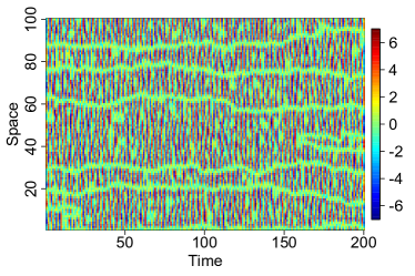
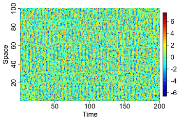
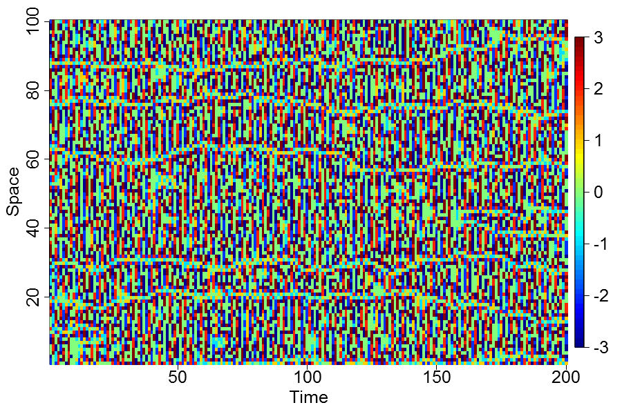
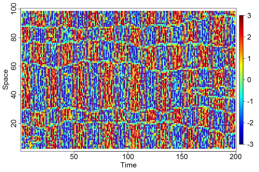
Figure 2 shows one realization of (19)–(20). The latent states have clear spatial structures, which is obscured in the observed field. Figure 3a shows the true predictive state space $S\left(\mathbf{r},t\right)$ (expected value at each at each $\left(\mathbf{r},t\right)$); the LICORS estimate $\widehat{S}\left(\mathbf{r},t\right)$ is shown in Fig. 3b. LICORS not only accurately estimates $S\left(\mathbf{r},t\right)$, but also learns the prediction rule (19) from the observed field $X\left(\mathbf{r},t\right)$.

5.1 Forecasting Competition: AR, VAR, and LICORS

A brute-force approach to spatio-temporal prediction would treat the whole spatial configuration at any one time as a single high-dimensional vector, and then use ordinary, parametric time-series methods such as vector auto-regressions (VAR) Luetkepohl07, or non- or semi- non-parametric models Bosq-nonparametric,Fan-Yao-time-series. Such global approaches suffer under the curse of dimensionality: real data sets may contain millions of space-time points, so fitting global models becomes impractical, even with strong regularization Bosq-Blanke-large-dim. Moreover, such global models will not be good representations of complex spatial dynamics.

On the other hand, space can be broken up into small patches (in the limit, single points), and then one can fit standard time series models to each patch’s low-dimensional time series. Such local strategies (partially) lift the curse of dimensionality, and thus make VAR or non-parametric time-series prediction practical, but creates the problem of selecting good sizes and shapes for these patches, and ignores spatial dependence across patches.

To show how LICORS escapes this dilemma, we compare it to other forecasting techniques in a simulation. Using $100$ replications of (19) – (20), with $n=100$ points in space, and $T=200$ steps in time, we compared LICORS, with and without pre-clustering, to (a) the empirical time-average of each spatial point; (b) a separate, univariate $AR(p)$ model for each point; a (c) separate $VAR(p)$ for each non-overlapping spatial patch of $5$ points; and the true conditional expectation function. (See §B.1 in the Supplemental Information for details of the competing methods.)

(a) In-sample

(b) Out-of-sample

Figure 4: MSEs for LICORS and parametric competitors on (19)–(20). LICORS with pre-clustering used $K=200$ clusters and varying past horizons; LICORS without pre-clustering use $k=50$ neighbors and $h_{p}=2$; both variants fixed $\alpha=0.05$.

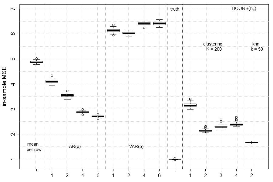
Figure 4 shows for each predictor the estimated mean squared error (MSE) for the in-sample (Fig. 4a) as well as out-of-sample (Fig. 4b) one-step ahead prediction error. Splitting up space while using standard methods appears not to help and may even hurt. LICORS performs best among all methods, once $h_{p}\geq 2$. While pre-clustering performs worse than direct estimation, it still predicts much better than the other methods.

Overall, LICORS with $h_{p}=2$ gives the best forecasts, where $\alpha=0.05$ was set in advance. At no point did we make an assumption about the number of predictive states or the shape of the conditional distribution. Even though the true system is conditionally Gaussian, LICORS out-performed the parametric Gaussian models. Thus we expect to do even better on non-Gaussian fields.

Even though we know the true light cone size in simulations, the “true” $\alpha$ can not be obtained directly. It controls the number of estimated predictive states: larger $\alpha$ implies less merging of clusters, and thus more number of predictive states; smaller $\alpha$ leads to more merging and hence less states.

In practice, one does not know the true light cone size nor the true number of states; they are rather control settings which affect the predictive performance. As we can accurately measure predictive performance by out-of-sample MSE, we propose a cross-validation (CV) procedure to tune $h_{p}$ and $\alpha$.

5.2 Cross-validation to Choose Optimal Control Settings

A good method should learn the invariant predictive structures of the system, avoiding over-fitting to the accidents of the observed sample. Ideally, the method should estimate nearly the same predictive states from (almost) any two realizations of the same system, while still being sensitive to differences between distinct systems.

Cross-validation is the classic way to handle this sensitivity-stability trade-off, and we use a data-set splitting version of it here. We simply divide the data set at its mid-point in time, use its earlier half to find predictive states, and evaluate the states’ performance on the data’s later half; see Supplemental Figure 7. (Assumption 7, of conditional stationarity, is important here.) While quite basic, simulations show that it does indeed find good control settings.

Using the same realizations of the model system as in the forecasting competition, we tried all combinations of $h_{p}\in\{1,2,3\}$ and $\alpha\in\{0.3,0.2,0.15,0.1,0.05,0.01,0.001\}$. We picked the control settings to do well on the continuation of the sample realization, but since this is a simulation, we can also check that these settings perform well on an independent realization of the same process. Figure 5 compares, for the selected control settings, the in-sample MSE on the first half of each realization, the MSE on the second half, and the MSE on all of a completely independent realization, for both the direct and the pre-clustered versions of LICORS. (As before, direct estimation does a bit better than pre-clustering.) There is little difference between the MSEs on the continuation of the training data and on independent data, indicating little over-fitting to accidents of particular sample paths. (See §B.2 in the supplemental information for further details.) Notably, CV picked the optimal $h_{p}$, namely 2, on all 100 trials.

Figure 5: Cross-validation for LICORS: MSE, using the CV-picked control settings, on the first half of each realization (“in-sample”), on the second half (“future”), and on all of an independent realization (“independent”).

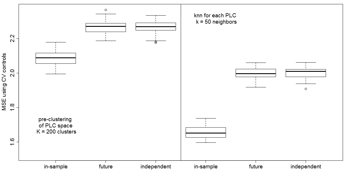
As expected, the smaller the value of $\alpha$ picked by CV, the more merging between clusters, and the smaller the number of states (see Supplemental Figure 8). Here, the true number of states $m=7$, but both pre-clustering and direct estimation give much higher $\widehat{m}$ (10–30 with pre-clustering, 30–90 without). The gap appears to be due to cross-validating pushing (in this context) for lower approximation error and more states, rather than fewer states and lower estimation error (§B.2 in the supplemental information). Having $\widehat{m}$ be substantially larger than $m$ thus does not degrade out-of-sample predictions.

6 Discussion

6.1 Related Work

Predictive state reconstruction estimates the prediction processes introduced by Knight-predictive-view. Knight’s construction is for stochastic processes $X$ with a single, continuous time index; but since $X_{t}$ can take values in infinite-dimensional spaces, most useful spatial models can implicitly be handled in this way, and by considering discrete time we avoid many measure-theoretic complications. After Knight, the same basic construction of the prediction process was independently rediscovered in nonlinear dynamics and physics Inferring-stat-compl,CMPPSS, in machine learning Jaeger-operator-models,predictive-representations-of-state,Langford-Salakhutdinov-Zhang, and in the philosophy of science Salmon-1984.

Spatio-temporally local prediction processes were introduced in CRS-prediction-on-networks,QSO-in-PRL to study self-organization and system complexity, along lines suggested by Grassberger-1986,Inferring-stat-compl. A related proposal was made by was made by Parlitz-Merkwirth-local-states, and light cones have been used in stochastic models of crystallization Capasso-Micheletti-spatial-birth-growth, going back to Kolmogorov-light-cones.

While the prediction-process formalism allows for continuous-valued observable fields, the prior work by Shalizi et al. only gave procedures for discrete-valued fields. Jänicke et al. used those procedures on continuous-valued data by discretizing them Jaenicke09_Diss,Janicke-Scheuermann-automatic-visualization,Jaenicke-et-al-multifield-visualization. We avoid discretization by using methods to estimate and compare continuous, high-dimensional distributions.

6.2 Conclusion

We introduce a new non-parametric method, LICORS, for spatio-temporal prediction. LICORS learns the predictive geometry in the state space underlying the system, by clustering observations according to the similarity of their local predictive distributions. Together with our cross-validation scheme, LICORS is a fully data-driven, non-parametric method to learn and use the non-linear, high-dimensional dynamics of a large class of spatio-temporal systems. The good performance of the CV procedure (Fig. 7) suggests that using it to find control settings in applications will avoid over-fitting.

Under weak assumptions, LICORS consistently estimates predictive distributions. Simulations show that it largely outperforms standard prediction methods. We have motivated presented results for $(1+1)D$ fields, but both the theory and practice extend without modification to higher-dimensional fields. While it will be good to extend LICORS to handle continuous predictive states, and to derive theoretical guarantees about its behavior under cross-validation, it can already be applied to experimental data. It provides a powerful, principled tool for forecasting complex spatio-temporal systems.

plainnat ../../../bib/PhD_thesis,../../../bib/locusts

Supplementary Material for “LICORS: Light Cone Reconstruction of States for Non-parametric Forecasting of Spatio-Temporal Systems”

Appendix A Predictive States: Details on Methodology, Implementation, and Algorithms

1. Collect the PLC and FLC configurations, $\ell^{-}\left(\mathbf{r},t\right)$ and $\ell^{+}\left(\mathbf{r},t\right)$, for each $\left(\mathbf{r},t\right)$ in the observed field $X\left(\mathbf{r},1\right),\ldots,X\left(\mathbf{r},T\right)$. 2. To cluster or not to cluster: (a) Assign each point to its own cluster. Only for small $N$ this is computationally feasible. (b) Perform an initial clustering (e.g. (e.g., K-means++ k-means-plus-plus) in the PLC configuration space (Section 3.1). 3. For each pair of clusters, test whether the estimated conditional FLC distributions are significantly different, at some fixed level $\alpha$ (Section 3.2). If not, merge them and go on. Stop when no more merges are possible. 4. Treat the remaining clusters as predictive states, and estimate the conditional distributions over FLC configurations. 5. Return the partition of PLC configurations into predictive states, and the associated predictive distributions.

Figure 6: Estimating predictive states from continuous-valued data: in 2a conditional distributions are tested for each $\ell^{-}_{i}$, $i=1,\ldots,N$, using a $\delta$-neighborhood (or $k$ nearest neighbors) of $\ell^{-}_{i}$ (see Section 4.1.1 for details); 2b uses an initial clustering to reduce complexity of the testing problem from $\mathcal{O}(N^{2})$ to $\mathcal{O}(K^{2})$ (see also Section 3.1).

Algorithm 1 Test equality of conditional predictive FLC distributions $\mathbb{P}\left(L^{+}\mid\text{clusterID}=k\right)$

0:  

  

Data:
$\mathbf{F}=\{\ell^{+}_{i}\}_{i=1}^{N}\in\mathbb{R}^{N\times n_{f}}$	$\ldots$	array with FLCs
clusterID	$\ldots$	labels of the PLC partitioning (step 2a or 2b in Fig. 6)
Parameters:
$\alpha\in[0,1]$	$\ldots$	significance level $\alpha$ for testing $H_{0}:\mathbb{P}\left(L^{+}\mid\ell^{-}_{i}\right)=\mathbb{P}\left(L^{+}\mid\ell^{-}_{j}\right)$

  

  $k_{\max}=\max$ clusterID

  for $k=1,\ldots,k_{\max}$ do

     fetch FLC samples given partition $P_{k}$: $\mathbf{F}_{k}=\{\ell^{+}_{i}\}_{\{i\mid clusterID[i]==k\}}$

     j = k

     lasttested = 0

     pvalue = 1

     while pvalue $>\alpha$ or $j\leq k_{\max}$ do

        j = j+ 1

        lasttested = j

        fetch FLC samples given partition $P_{j}$: $\mathbf{F}_{j}=\{\ell^{+}_{i}\}_{\{i\mid clusterID[i]==j\}}$

        pvalue $\leftarrow test(\mathbb{P}\left(L^{+}\mid P_{k}\right)=\mathbb{P}\left(L^{+}\mid P_{j}\right)\mid\mathbf{F}_{k},\mathbf{F}_{j})$

        if pvalue $<\alpha$ then

           merge cluster $j$ with cluster $k$: clusterID[clusterID == j] = k After no merging is possible clusterID contains the labels of the predictive states.

  return  clusterID

We partition the observed PLCs $\{\ell_{i}^{-}\}_{i=1}^{N}\subset\mathbb{R}^{n_{p}}$ into $K=K(\delta)$ disjoint groups $\{P_{k}\}_{k=1}^{K}$, choosing the number of groups so that all have diameters less than $\delta$. This choice of $K(\delta)$ guarantees (Assumption 3.1) that all $\ell^{-}\in P_{k}$ have predictive distributions that are at most $\rho$ apart. Thus all PLCs within a group $P_{k}$ are (nearly) equivalent by Definition 2.1. This in turn means we only need to compare predictive distributions between clusters.

A.1 Lebesgue Smoothing

In a standard kernel regression approach one would compute a similarity measure on PLCs $\ell^{-}_{i}$ and then use a weighted mean of FLCs $\ell_{i}^{+}$ to get a point prediction of the future cone, i.e.,

$$\widehat{L^{+}}\left(\mathbf{r},t\right)=\sum_{\left(\mathbf{q},\tau\right)}{w^{-}\left(\mathbf{q},\tau;\left(\mathbf{r},t\right)\right)\ell^{+}\left(\mathbf{q},\tau\right)}\text{ for all }\tau<t,$$ (21)

where $w^{-}\left(\mathbf{q},\tau;\left(\mathbf{r},t\right)\right)\propto K^{-}\left(\lVert\ell^{-}\left(\mathbf{r},t\right)-\ell^{-}\left(\mathbf{q},\tau\right)\rVert\right)$ are normalized weights determined by a kernel $K^{-}\left(\cdot\right)$ in the PLC configuration space. For example, a Gaussian kernel $K_{h}^{-}\left(\ell^{-}\left(\mathbf{r},t\right),\ell^{-}\left(\mathbf{q},\tau\right)\right)=\exp(-\frac{1}{h}\lVert\ell^{-}\left(\mathbf{r},t\right)-\ell^{-}\left(\mathbf{q},\tau\right)\rVert_{2}^{2})$ with squared Euclidean distance and bandwidth $h$.

Since $\left(\mathbf{q},\tau\right)$ ranges over the entire space-time, $\mathbf{q}\in\mathbf{S}$, $\tau=1,\ldots,t-1$, computing this many similarities $\{s_{\left(\mathbf{q},\tau\right),\left(\mathbf{r},t\right)}\}$ becomes very time consuming. A typical $10$-second video might have $N=3\cdot{10}^{7}$ space-time points. To evaluate (21) needs $3\cdot 10^{7}$ similarities in $n_{p}$-dimensional space — and this just to predict one FLC. If $N$ is large, then predictive state estimation is a necessary pre-step before making predictions.

Our approach differs in two important ways. First, we assume a discrete predictive state space which is sufficient to predict the future. Thus once we have estimated the predictive states $\epsilon_{1},\ldots,\epsilon_{m}$, we can predict the field at any $\left(\mathbf{r},t\right)$ using the average (or mode) of the estimated predictive state at $\left(\mathbf{r},t\right)$,

$$\widehat{L^{+}}\left(\mathbf{r},t\right)=\mathbb{E}_{\widehat{\epsilon}\left(\ell^{-}\left(\mathbf{r},t\right)\right)}\left(L^{+}\left(\mathbf{r},t\right)\right).$$ (22)

Second, we learn a new geometry on the PLC space by defining closeness in the FLC distribution space, rather than in the PLC configuration space. Thus a natural continuous state space extension of (22) is a Kernel regression with weights that depend on the similarity in the output rather than the input space, i.e.

$$\widehat{L^{+}}\left(\mathbf{r},t\right)=\sum_{\left(\mathbf{q},\tau\right)}{w^{+}\left(\mathbf{q},\tau;\left(\mathbf{r},t\right)\right)\ell^{+}\left(\mathbf{q},\tau\right)}\text{ for all }\tau<t,$$ (23)

where the normalized weights $w^{+}\left(\mathbf{q},\tau;\left(\mathbf{r},t\right)\right)\propto K^{+}\left(\lVert\mathbb{P}\left(\ell^{+}\left(\mathbf{r},t\right)\right)-\mathbb{P}\left(\ell^{+}\left(\mathbf{q},\tau\right)\right)\rVert\right)$ are based on a Kernel $K^{+}\left(\cdot\right)$ in the FLC distribution space.

One can generalize (23) to the classic non-parametric regression setting $y=m(x)+u$ and define a new Kernel regression estimator as

$$\widehat{m}^{(L)}(x)=\sum_{i=1}^{n}{\frac{K_{y}\left(\widehat{m}^{(R)}(x_{i})-m(x)\right)}{h_{y}}y_{i}}~{},$$ (24)

where $\widehat{m}^{(R)}(\cdot)$ serves as a pilot estimate; for example the classic kernel regression smoother

$$\widehat{m}^{(R)}(x)=\sum_{i=1}^{n}{\frac{K_{x}\left(x_{i}-x\right)}{h_{x}}y_{i}}~{}.$$ (25)

As we average over nearby predictions rather than nearby inputs, we may call (24) “Lebesgue smoothing”, in contrast to the “Riemann” smoothing of (25). If $N$ is small, then we can forecast with (23) forecast without estimating predictive states. However, here we focus on predictive-state recovery, and leave Lebesgue smoothed LICORS to future work.

Further performance enhancements for testing

While it is better to do $\mathcal{O}(K^{2})$ high-dimensional tests than $\mathcal{O}(N^{2})$, it would be better still to speed up each test. Since two distributions are the same only if their moments are, we can start by testing simply for equality of means, which is fast and powerful, and do a full distributional test only if we cannot reject on that basis. For multivariate mean tests we can use the Hotelling test ABW98 and its randomized generalization Lopes-et-al-randomized-Hotelling-test. Yet another strategy to reduce the number of costly high-dimensional, non-parametric tests is to test various functions $f(\cdot)$ of the samples. If the distributions of $\mathbf{F}_{k_{i}}(\delta)$ and $\mathbf{F}_{k_{j}}(\delta)$ are the same, then also $\mathbb{P}\left(f\left(\mathbf{F}_{k_{i}}(\delta)\right)\right)=\mathbb{P}\left(f\left(\mathbf{F}_{k_{j}}(\delta)\right)\right)$ for any measurable $f$. Particularly, we can apply random projections Lopes-et-al-randomized-Hotelling-test to $\mathbf{F}_{k_{i}}$ to go from the high-dimensional $\mathbb{R}^{n_{f}}$ down to the one-dimensional $\mathbb{R}$, followed by a Kolmogorov-Smirnov test. Only if these tests can not reject equality for several projections, one uses fully non-parametric tests.

Appendix B The Simulation and the Forecasting Competition

B.1 Details of Competing Methods

The local VAR models were fit with Lasso regularization BickelSong11_LargeVAR, as implemented in the fastVAR package fastVAR. We also tried un-regularized VAR models, but they performed even worse.

1. Split dataset at its middle in time: $\mathcal{D}_{1}=\{X\left(\mathbf{r},t\right)\}_{t=1}^{T/2}$ and $\mathcal{D}_{2}=\{X\left(\mathbf{r},t\right)\}_{t=T/2+1}^{T}$ 2. For each combination of control settings, do: (a) Training: estimate predictive states from $\mathcal{D}_{1}$ (b) Test-set prediction: find predictive state of each PLC $\in\mathcal{D}_{2}$ and predict its FLC $\in\mathcal{D}_{2}$. (c) Error: compare to the observed FLCs $\in\mathcal{D}_{2}$ and compute the loss. 3. Choose the control settings with the smallest test-set loss.

Figure 7: Cross-validation to choose control settings given data $\{X\left(\mathbf{r},t\right)\}_{t=1}^{T}$.

B.2 Excess Risk, Test Size, and Number of Estimated States

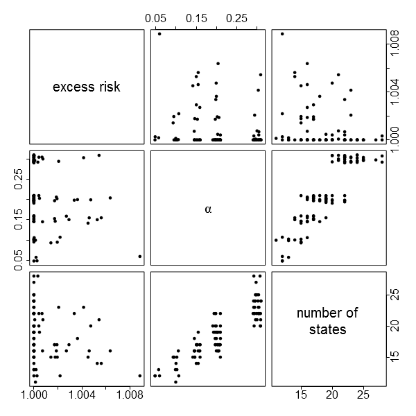
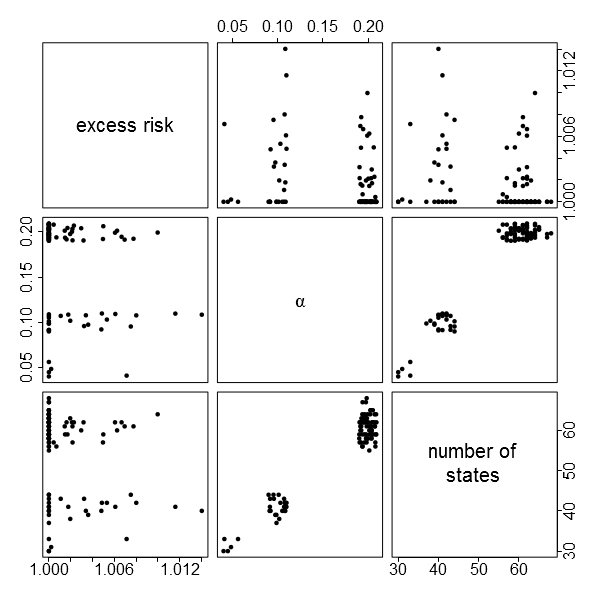
Figs. 8a and 8b show the expected relationship between $\alpha$ and the number of predictive states recovered $\widehat{m}$: smaller $\alpha$ leads to more merging, and fewer states. Here the true number of states $m=7$, but both pre-clustering and direct estimation give much higher $\widehat{m}$. Thus for LICORS, optimal forecasting pushes for more states and lower approximation error, rather than fewer states and lower estimation error. We can check this explanation by considering the ratio

$$\text{excess risk}:=\frac{\text{MSE(sample $i+1$)}\text{ using }(h_{p},\alpha)_{i,CV_{i}}}{\text{MSE(sample $i+1$)}\text{ using }(h_{p},\alpha)_{i+1,\min}}\geq 1.$$ (26)

Recall that $(h_{p},\alpha)_{i,CV_{i}}$ is chosen using only sample $i$, while $(h_{p},\alpha)_{i+1,\min}$ is the minimizing pair after having evaluated the MSE on sample $i+1$. The best that any data-driven procedure could do would be to guess $(h_{p},\alpha)_{i+1,\min}$ from sample $i$, so the excess risk is $\geq 1$, with equality only if CV picked the optimal control settings. The scatter-plots show that our CV procedure has an excess risk on the order of $10^{-2}$ compared to the oracle pair. Hence, even though $\widehat{m}$ is substantially larger than $m$, the difference is practically irrelevant for predictions.

(a)

(b)

Figure 8: Relations between excess risk, test size, and the number of reconstructed states for LICORS: (a) selected $\alpha$, number of estimated states, and excess risk (Eq. (26)) for pre-clustered LICORS; (b) the same for direct-estimation LICORS. $\alpha$ values in are jittered.

B.3 Discussion of the Simulations

The simulations showed that LICORS outperforms standard forecasting techniques by a large margin, even though it presumes very little about the data source. Especially note that the out-of-sample MSE in Fig. 5 is still much lower than the best parametric in-sample MSE in Fig. 4a — even though it uses only half the sample size. The good performance of the CV procedure (Fig. 7) suggests that using it to find control settings in applications will avoid over-fitting.

In real applications $N$ would typically on the order of millions (rather than merely $2\times{10}^{4}$), making pre-clustering essential computationally — at least until $\operatorname{\mathcal{O}}\bigl{(}N^{2}\bigr{)}$ comparisons for millions of data points become tractable. Pre-clustering usually leads to a performance loss as it hides fine structures in the predictive distribution space (see also the remark below Lemma 4.7). However, the in-sample and out-of-sample MSE comparison showed that this performance loss is small compared to the gain over standard parametric methods, and further attenuated with CV.

Appendix C Proofs

Proof of Lemma 4.5.

$$\mathbb{P}\left(L^{+}\left(\mathbf{r},t\right),L^{+}\left(\mathbf{u},s\right)\mid S\left(\mathbf{r},t\right),S\left(\mathbf{u},s\right)\right)$$ (27)

$$= \mathbb{P}\left(L^{+}\left(\mathbf{r},t\right)\mid L^{+}\left(\mathbf{u},s\right),S\left(\mathbf{r},t\right),S\left(\mathbf{u},s\right)\right)\mathbb{P}\left(L^{+}\left(\mathbf{u},s\right)\mid S\left(\mathbf{r},t\right),S\left(\mathbf{u},s\right)\right)$$ (28)

$$= \mathbb{P}\left(L^{+}\left(\mathbf{r},t\right)\mid L^{+}\left(\mathbf{u},s\right),S\left(\mathbf{r},t\right),S\left(\mathbf{u},s\right)\right)\mathbb{P}\left(L^{+}\left(\mathbf{u},s\right)\mid S\left(\mathbf{u},s\right)\right)$$ (29)

$$= \mathbb{P}\left(L^{+}\left(\mathbf{r},t\right)\mid S\left(\mathbf{r},t\right)\right)\mathbb{P}\left(L^{+}\left(\mathbf{u},s\right)\mid S\left(\mathbf{u},s\right)\right)~{},$$ (30)

The first equality is simple conditioning, the second equality holds since given the predictive state at $\left(\mathbf{u},s\right)$ the distribution of $L^{+}$ is independent of the predictive state at another $\left(\mathbf{r},t\right)$, and the last equality holds for the same reason as the second plus the non-overlap of the FLCs at $\left(\mathbf{r},t\right)$ and $\left(\mathbf{u},s\right)$. ∎

Proof of Corollary 4.6.

The FLC of $\left(\mathbf{r},t\right)$ with $h_{f}=0$ is just the single point $X\left(\mathbf{r},t\right)$. Since two univariate FLCs cannot overlap unless they are equal, the result follows immediately from Lemma 4.5. ∎

Proof of Lemma 4.7.

By contradiction. Assume that $\ell_{j}^{-}$ and $\ell^{-}_{k}$, with $j,k\in I_{i}(\delta)$, have different predictive states, without loss of generality $\epsilon_{1}$ and $\epsilon_{2}$. By Assumption 4.4, then, $\mathcal{D}_{KL}\left(\epsilon_{1}\mid\mid\epsilon_{2}\right)$ and $\mathcal{D}_{KL}\left(\epsilon_{2}\mid\mid\epsilon_{1}\right)$ are both at least $d_{\min}$. By the definition of $I_{i}(\delta)$, $\lVert\ell_{j}^{-}-\ell_{k}^{-}\rVert<2\delta$. By Assumption 3.1, then, $\mathcal{D}_{KL}\left(\epsilon_{1}\mid\mid\epsilon_{2}\right)$ and $\mathcal{D}_{KL}\left(\epsilon_{2}\mid\mid\epsilon_{1}\right)$ are both at most $\rho(2\delta)$. But by making $\delta$ sufficiently small, $\rho(2\delta)$ can be made as small as desired, and in particular can be made less than $d_{\min}$. This is a contradiction, so all the past cone configurations in $I_{i}(\delta)$ must be predictively equivalent. ∎

Proof of Corollary 4.8.

Immediate from combining Lemmas 4.7 and 4.5. ∎

Proof of Theorem 4.12.

Before going into the formal proof, we make an observation regarding non-parametric two-sample tests. Most of these, to have good operating characteristics, require independent samples. Since we will be applying the tests to $\mathbf{F}_{i}(\delta)$ and $\mathbf{F}_{j}(\delta)$,

Properties C.1 (Pairwise independent samples).

If

$$I_{i}(\delta)\cap I_{j}(\delta)=\emptyset.$$ (31)

then the samples $\mathbf{F}_{i}(\delta)$ are independent of $\mathbf{F}_{j}(\delta)$, $j\neq i$ (see (14)).

Let $\Delta_{ij}:=\lVert\ell_{i}^{-}-\ell_{j}^{-}\rVert$. If $\Delta_{ij}>2\delta$, then (31) is satisfied. If $\Delta_{ij}<2\delta$, then a sample in $\mathbf{F}_{i}(\delta)$ might also appear in $\mathbf{F}_{j}(\delta)$ and therefore violate the independence assumption for two sample tests.

For these rare cases redefine the index set $I_{i}(\delta)$ and $I_{j}(\delta)$ such that (31) holds. We can achieve this by excluding the intersection, split it in half ( $\pm 1$ sample), and then re-assign these halves to each index set. For all pairs $i\neq j$ determine $I_{i}(\delta)\cap I_{j}(\delta)=:I_{i\cap j}(\delta)$. Then let

$$I_{i} :=I_{i}\setminus I_{i\cap j}\cup\{i_{1},\ldots,i_{|I_{i\cap j}|/2}\mid i_{k}\in I_{i\cap j}\}$$ (32)

$$\text{ and }I_{j} :=I_{j}\setminus I_{i\cap j}\cup\{i_{|I_{i\cap j}|/2},\ldots,i_{|I_{i\cap j}|}\mid i_{k}\in I_{i\cap j}\}.$$ (33)

If $I_{i\cap j}=\emptyset$, (32)–(33) does not change the index set; if $I_{i\cap j}\neq\emptyset$, then (32)–(33) guarantees an empty intersection.

The proof of consistency relies crucially on a growing index set $I_{i}$. The re-definition in (32)–(33) does not change the rate at which $S_{i}(N,\delta)$ grows, because in the worst case (for very close PLCs) it just divides $s_{i}(N,\delta)$ and $s_{j}(N,\delta)$ in half.

Proof:

We first bound the error for each row $\widehat{\mathbf{A}}_{i}$, and then use a union bound for the probability of error for $\widehat{\mathbf{A}}$.

Bound error per row

For each row $T_{n,m}$ tests $H_{0}:\ell_{i}\sim\ell_{j}$, $j>i$ (due to symmetry the cases $j<i$ have already been tested before) based on the sample $\mathbf{F}_{i}(\delta)\sim\epsilon_{i}$ and $\mathbf{F}_{j}(\delta)\sim\epsilon_{j}$. The worst-case distance $d$ for the non-parametric test in Assumption 4.11 is $d=d_{\min}$. For simplicity consider the first row: here we have to make $N-1$ tests, of which $N_{1}-1$ should correctly accept, and $N-N_{1}$ should correctly reject equality of distributions.

$$\mathbb{P}\left(\widehat{\mathbf{A}}_{j}\neq\mathbf{A}_{j}\right) \leq (N_{j}-1)\mathbb{P}\left(\left(\text{type I}\right)+(N-N_{j})\right)\mathbb{P}\left(\text{type II}\right)$$ (34)

$$\leq (N_{j}-1)\alpha+(N-N_{j})\beta\left(\alpha,S_{\min}(N,\delta),S_{\min}(N,\delta)\right)$$ (35)

$$\leq N_{j}\alpha+(N-N_{j})\beta\left(\alpha,S_{\min}(N,\delta),S_{\min}(N,\delta)\right)$$ (36)

since the worst case, for type II error, is that both samples are as small as possible.

Bound error for entire matrix

The probability of error for the entire predictive state clustering can again be bounded using the union bound:

$$\mathbb{P}\left(\widehat{\mathbf{A}}\neq\mathbf{A}\right) =\mathbb{P}\left(\bigcup_{j=1}^{N}{\{\widehat{\mathbf{A}}_{j}\neq\mathbf{A}_{j}\}}\right)$$ (37)

$$\leq\sum_{j=1}^{N}{\mathbb{P}\left(\widehat{\mathbf{A}}_{j}\neq\mathbf{A}_{j}\right)}$$ (38)

$$\leq N\left(N_{\max}\alpha+(N-N_{\min})\beta\left(\alpha,S_{\min}(N,\delta),S_{\min}(N,\delta)\right)\right)$$ (39)

$$=NN_{\max}\alpha+(N^{2}-NN_{\min})\beta\left(\alpha,S_{\min}(N,\delta),S_{\min}(N,\delta)\right),$$ (40)

where $N_{\max}=\max_{j}N_{j}$ is the number of light cones in the largest predictive state.

Under Assumption 4.11, $\alpha$ and $\beta$ are both $\operatorname{o}\bigl{(}NN_{\max}\bigr{)}$, so the over-all arrow probability tends to zero. ∎

plainnat ../../../bib/PhD_thesis,../../../bib/locusts