Einstein–Podolsky–Rosen correlations from colliding Bose–Einstein condensates

Abstract

We propose an experiment which can demonstrate quantum correlations in a physical scenario as discussed in the seminal work of Einstein, Podolsky and Rosen. Momentum-entangled massive particles are produced via the four-wave mixing process of two colliding Bose–Einstein condensates. The particles’ quantum correlations can be shown in a double double-slit experiment or via ghost interference.

.1 I. Introduction

Since the seminal works of Einstein, Podolsky and Rosen (EPR) Eins1935 and Schrödinger Schr1935 numerous experiments have demonstrated the counter-intuitive effects of quantum entanglement, in particular the violation of local realism through Bell’s inequality Bell1964 . Entanglement has been demonstrated for many physical systems such as photons Free1972 ; Aspe1982 ; Kwia1995 , atoms Hagl1997 ; Gros2011 , ions Turc1998 ; Rowe2001 , and superconducting devices Stef2006 . Variants of the EPR experiment have been realized, for example exploiting the analogy with quadrature phase operators Ou1992 . But, until now, nobody was able to demonstrate the original EPR idea of an entangled state of freely moving massive particles in their external degrees of freedom, i.e. a state of the form $\int_{-\infty}^{\infty}$d$x\,\left|x\right\rangle_{\text{A}}\left|x\!+\!x_{0}\right\rangle_{\text{B}}=\int_{-\infty}^{\infty}$d$p\,$exp$(\tfrac{\text{i}}{\hbar}x_{0}p)\,\left|p\right\rangle_{\text{A}}\left|-p\right\rangle_{\text{B}}$, where, $x$ and $p$ denote position and momentum, $x_{0}$ is a constant, and indices label the two particles.

In this proposal, following the experimental approach of Ref. Perr2007 , we consider a Bose–Einstein condensate (BEC) of metastable helium-4 (⁴He^∗). Via interactions with lasers, the particles are outcoupled from the trap, brought to collision, and fall on a detector. The collisions prepare atom pairs in a three-dimensional version of the EPR state with fixed absolute momenta. While the idealized EPR state would have to be created everywhere in space, our pairs are created in a finite space volume. We propose to test the entanglement in a double double-slit experiment or via ghost interference.

We start with a short review of the procedure described in Ref. Perr2007 : ⁴He^∗ atoms of mass $m\simeq 6.646\!\cdot\!10^{-27}\,$kg are magnetically trapped and form a cigar-shaped BEC along the (horizontal) $x$ direction. One employs two $\sigma$-polarized laser beams counterpropagating horizontally along the $+x$ and $-x$ directions and a $\pi$-polarized laser beam from the top along the $-z$ direction fulfilling the Raman condition, all with a wavelength $\lambda_{\text{L}}\simeq 1.083\,$ µm. They bring the atoms into a magnetically insensitive state and thereby induce a velocity kick in the horizontal $\pm x$ directions and a kick upwards along $+z$. The recoil velocity of each kick is $v_{\text{rec}}=\tfrac{h}{\lambda_{\text{L}}\,m}\simeq 92\,$mm$/$s, where $h$ is Planck’s constant. Thus, the three laser beams produce a superposition of two counterpropagating matter waves of falling helium atoms, which subsequently scatter in a four-wave mixing process. In total, a fraction of about 5 % of all $10^{4}$ to $10^{5}$ helium atoms collides and is scattered from the two condensates. While the relative velocity of two scattered atoms is $2\,v_{\text{rec}}$, the velocity uncertainties can be obtained from the Gross-Pitaevskii equation. Assuming the trap parameters of Ref. Perr2007 , the BEC is elongated along $\pm x$ and the uncertainties are anisotropic: $\Delta v_{x}\simeq 0.0044\,v_{\text{rec}}$, $\Delta v_{y,z}\simeq 0.091\,v_{\text{rec}}$.

The collisions are, to a very good approximation, of s-wave type, i.e. isotropic, and take place over a characteristic timescale of $150\,$ µs Perr2007 . Depending on the size of the condensate the collisions can produce momentum correlated particle pairs, lying on a shell in velocity space, whose origin is at $v_{\text{rec}}\,\mathbf{\hat{e}}_{z}$ with radius $v_{\text{rec}}$. Within quantum mechanical uncertainties, momentum conservation requires the two partners to find themselves being anticorrelated to each other in momentum space. Most importantly, the isotropic nature of the s-wave scattering process gives rise to the superposition of all possible emission directions and thus to quantum mechanical entanglement in the external degrees of freedom of the two massive particles.

The atomic de Broglie wavelength $\lambda_{\text{dB}}$ associated with the recoil velocity is the same as the wavelength of the laser beams: $\lambda_{\text{dB}}=\tfrac{h}{m\,v_{\text{rec}}}\simeq 1.083\,$ µm. In Refs. Molm2008 and Perr2008 a model for the observed Hanbury-Brown Twiss (collinear) and back-to-back (BB) correlations of Ref. Perr2007 is developed.

.2 II. Double double-slit experiment

Now consider a double double-slit arrangement as in Figure 1. All particles hit by the lasers get a velocity kick of $v_{\text{rec}}$ in the $\pm x$ direction as well as upwards along $+z$. Let us consider only those particles which collided in such a way that they did not get any additional vertical velocity component and are moving along $\pm y$ direction with velocity $v_{\text{rec}}$ after the collision (i.e. along $\pm\mathbf{\hat{e}}_{y}+\mathbf{\hat{e}}_{z}$ with velocity $\!\sqrt{2}\,v_{\text{rec}}$). With gravity acceleration $g\simeq 9.81\,$m$/$s² and distance to the detector $H=0.5\,$m, the falling time is $\tau\simeq 328.8\,$ms. Having the coordinate origin $\mathbf{O}$ in the center of the initial condensate, the atoms pass the double-slit at a lateral position of $y=L_{1}$ at some height $-h$ and hit the detector at the maximally possible lateral distance $y=L_{1}+L_{2}=v_{\text{rec}}\,\tau\simeq 30.2\,$mm.

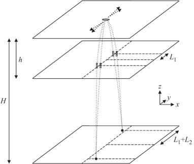
Figure 1: Schematic of the double double-slit experiment (not drawn to scale). Pairs of atoms collide at height $H$ and fall under gravity through the double slits onto the detector. See main text for details.

We can ignore the effect of gravity by considering only the top view of the experiment (Figure 2). The source S of size $S_{x}\times S_{y}\times S_{z}$ is emitting particle pairs A and B with velocity $v_{\text{rec}}$. At a distance $L_{1}$, there are two double-slits with slit separation $d$. At a further distance $L_{2}$ an observation screen is located. There are four possible paths for getting a coincidence between atom detections on the left and right side at positions $\mathbf{r}_{\text{A}}$ and $\mathbf{r}_{\text{B}}$ with $x$-coordinates $x_{\text{A}}$ and $x_{\text{B}}$, respectively: {$\mathbf{a}_{1}$,$\mathbf{b}_{1}$}, {$\mathbf{a}_{1}$,$\mathbf{b}_{2}$}, {$\mathbf{a}_{2}$,$\mathbf{b}_{1}$}, and {$\mathbf{a}_{2}$,$\mathbf{b}_{2}$}. Here {$\mathbf{a}_{i}$,$\mathbf{b}_{k}$} means particle A passed slit $\mathbf{a}_{i}$ and particle B passed slit $\mathbf{b}_{k}$ ($i,k=1,2$).

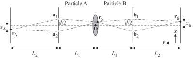
Figure 2: Schematic of the double double-slit experiment (top view, not drawn to scale). Pairs of atoms, A and B, are emitted from source points $\mathbf{r}_{\text{S}}$ within the BEC, pass double slits and arrive at detectors at positions $\mathbf{r}_{\text{A}}$ and $\mathbf{r}_{\text{B}}$. See main text for details.

As discussed in Refs. Horn1988 ; Gree1993 ; Horn1997 , there are two limiting cases in a double double-slit experiment:

1. If the source size is very small, there is no momentum correlation between the particles. The momentum spread of each individual particle is large enough so that it can go through either slit at the same time and its partner does not carry enough which-path-information to identify through which of them it went. Thus, each particle forms a Young pattern independently of its partner. One effectively has two single-particle interference patterns unrelated to entanglement. The far field double double-slit (dds) two-particle pattern at the observation screens is a product of two independent one-particle patterns and is of the form

   $$|\psi_{\text{AB}}^{\text{(dds)}}(x_{\text{A}},x_{\text{B}})|^{2}\propto\cos^{2}\!\left(\pi\dfrac{x_{\text{A}}}{d_{f}}\right)\cos^{2}\!\left(\pi\dfrac{x_{\text{B}}}{d_{f}}\right)$$ (1)

   with $d_{f}$ being the fringe distance.

2. If the source size is large (but still small compared to the slit distance), there is no one-particle interference pattern at either screen. The large source implies a small two-particle momentum uncertainty and therefore a high momentum correlation of the particle pairs. If one particle went through one slit, the other particle must have gone through the diagonally opposite one. However, since every particle is detected far behind a double-slit, the which-path information about its partner is erased. There is a superposition of two possibilities: particle A via upper slit & particle B via lower slit, and vice versa. The far field two-particle pattern cannot be factorized and has the form

   $$|\psi_{\text{AB}}^{\text{(dds)}}(x_{\text{A}},x_{\text{B}})|^{2}\propto\cos^{2}\!\left(\pi\dfrac{x_{\text{A}}\!-\!x_{\text{B}}}{d_{f}}\right).$$ (2)

   The Young fringes on, say, side B can be seen only conditionally on finding particles at a certain detector position $x_{\text{A}}$ on the left side. Only by measuring coincidences, an interference pattern can be seen. Its maximum on the right side is at the same $x$-position as the detector at the left side.

Importantly, there is also a third regime, namely the one of very large source size. If the condensate is comparable to or larger than the slit distance, the two-particle interference pattern arising from the diagonal paths {$\mathbf{a}_{1}$,$\mathbf{b}_{2}$} & {$\mathbf{a}_{2}$,$\mathbf{b}_{1}$} is superposed by a two-particle pattern originating from the horizontal paths {$\mathbf{a}_{1}$,$\mathbf{b}_{1}$} & {$\mathbf{a}_{2}$,$\mathbf{b}_{2}$}. Therefore, detection of one particle at either slit does not imply any information about the slit the other particle goes through. This restores one-particle interference and, due to complementarity, no genuine two-particle interference arises Jaeg1993 .

To calculate the two-particle interference pattern on the observation screen, we follow the treatment in Ref. Horn1997 , where one integrates over point sources which emit two spherical waves without any (anti)correlation in momentum. Remarkably, the anticorrelation and entanglement emerge naturally by integrating spherical waves of two particles emitted from the same position over a sufficiently large source area. This is in analogy to the Fourier transformation of a single particle in phase space, giving rise to reduced momentum uncertainty as the source grows larger. Let us denote the possible path lengths from $\mathbf{r}_{\text{S}}\equiv(x_{\text{S}},y_{\text{S}},z_{\text{S}})$ to $\mathbf{r}_{\text{A}}\equiv(x_{\text{A}},L_{1}+L_{2},0)$ and $\mathbf{r}_{\text{B}}\equiv(x_{\text{B}},-L_{1}-L_{2},0)$ by $L_{\mathbf{a}_{i}}\equiv\overline{\mathbf{r}_{\text{S}}\mathbf{a}_{i}}+\overline{\mathbf{a}_{i}\mathbf{r}_{\text{A}}}$ and $L_{\mathbf{b}_{i}}\equiv\overline{\mathbf{r}_{\text{S}}\mathbf{b}_{i}}+\overline{\mathbf{b}_{i}\mathbf{r}_{\text{B}}}$ with $i=1,2$, as calculated by simple geometry. The (unnormalized) quantum mechanical amplitude for two entangled particles, emerging from $\mathbf{r}_{\text{S}}$, to land at points $\mathbf{r}_{\text{A}}$ and $\mathbf{r}_{\text{B}}$ is

$$\psi_{\text{SAB}}^{\text{(dds)}}(\mathbf{r}_{\text{S}},\mathbf{r}_{\text{A}},\mathbf{r}_{\text{B}}) \propto\text{e}^{\text{i\thinspace}\frac{2\pi}{\lambda_{\text{dB}}}\,(L_{\mathbf{a}_{1}}+L_{\mathbf{b}_{1}})}+\text{e}^{\text{i\thinspace}\frac{2\pi}{\lambda_{\text{dB}}}\,(L_{\mathbf{a}_{1}}+L_{\mathbf{b}_{2}})}$$

$$\;\;\;\;+\text{e}^{\text{i\thinspace}\frac{2\pi}{\lambda_{\text{dB}}}\,(L_{\mathbf{a}_{2}}+L_{\mathbf{b}_{1}})}+\text{e}^{\text{i\thinspace}\frac{2\pi}{\lambda_{\text{dB}}}\,(L_{\mathbf{a}_{2}}+L_{\mathbf{b}_{2}})}.$$ (3)

It is a superposition of four equal-weight amplitudes corresponding to the possible path combinations of particles A and B. We have omitted the one-over-distance dependence of the amplitude of the spherical waves because it is practically constant in the far field and can be taken into the normalization factor. The phase of the amplitude of a collision to happen can be treated constant over the source volume if one neglects the expansion of the colliding BECs. Then, we can write down the quantum mechanical amplitude for two entangled particles, emerging from the whole source, to land at points $\mathbf{r}_{\text{A}}$ and $\mathbf{r}_{\text{B}}$. It is a superposition of all possible emission points over the source volume $V$ and is obtained via integration over the whole condensate, possibly with some weighting function $g(\mathbf{r}_{\text{S}})$:

$$\psi_{\text{AB}}^{\text{(dds)}}(\mathbf{r}_{\text{A}},\mathbf{r}_{\text{B}})\propto\dfrac{1}{V}\,{\displaystyle\iiint\nolimits_{\text{S}}}\,\text{d}\mathbf{r}_{\text{S}}\,g(\mathbf{r}_{\text{S}})\,\psi_{\text{SAB}}(\mathbf{r}_{\text{S}},\mathbf{r}_{\text{A}},\mathbf{r}_{\text{B}}).$$ (4)

Summing up, we have the following conditions for a two-particle interference experiment:

1. The source must be sufficiently large to achieve well defined momentum correlation and wash out the single-particle interference pattern:

   $$\dfrac{\Delta p_{x}}{p}\ll\dfrac{d}{L_{1}}.$$ (5)

   The relative momentum spread $\tfrac{\Delta p_{x}}{p}=\tfrac{\Delta p_{x}}{mv_{\text{rec}}}$ must be small enough not to “illuminate” both slits. The source size $S_{x}$ implicitly influences $\Delta p_{x}$. The larger the source size along $x$, the smaller $\Delta p_{x}$ becomes and the better the condition can be fulfilled.

2. The fringe distance $d_{f}$ should be much larger than the detector resolution $\delta x$:

   $$d_{f}=\lambda_{\text{dB}}\,\dfrac{L_{2}}{d}>5\,\delta x.$$ (6)

   Here we assume that one needs at least 5 pixels per oscillation.

3. The source must be sufficiently small not to destroy the two-particle interference pattern:

   $$S_{x}\ll d.$$ (7)

   If the source size becomes comparable to or larger than the slit distance, two two-particle interference patterns wash each other out.

Now we come to the parameter analysis. We take $\tfrac{\Delta p_{x}}{p}=\frac{1}{\pi}\sqrt{\frac{21}{8}}\,\frac{\lambda_{\text{dB}}}{S_{x}}\simeq\frac{0.56\,\mathrm{\SIUnitSymbolMicro}\text{m}}{S_{x}}$ Sten1999 and $S_{y}=10\,\mathrm{\SIUnitSymbolMicro}$m. This leaves $S_{x}$ as a free parameter, and we can write conditions (I), (II), and (III) in a single line:

$$0.56\,\mathrm{\SIUnitSymbolMicro}\text{m}\times\frac{L_{1}}{d}\;\overset{(\text{I})}{\ll}\;S_{x}\;\overset{(\text{III})}{\ll}\;d\;\overset{(\text{II})}{<}\;\frac{\lambda_{\text{dB}}\,L_{2}}{5\,\delta x}.$$ (8)

An approximate solution for all our simultaneous constraints is $d=100\,\mathrm{\SIUnitSymbolMicro}$m, $L_{1}=5\,$mm, $L_{2}=25\,$mm. Here $L_{1}+L_{2}$ exploits the maximal possible lateral distance given by the distance between BEC and detector of $H=0.5\,$m. The fringe distance becomes $d_{f}\simeq 271\,\mathrm{\SIUnitSymbolMicro}$m, which means that a fringe is resolved by only 4 to 5 pixels, given a detector resolution of $\delta x\simeq 60\,$ µm.

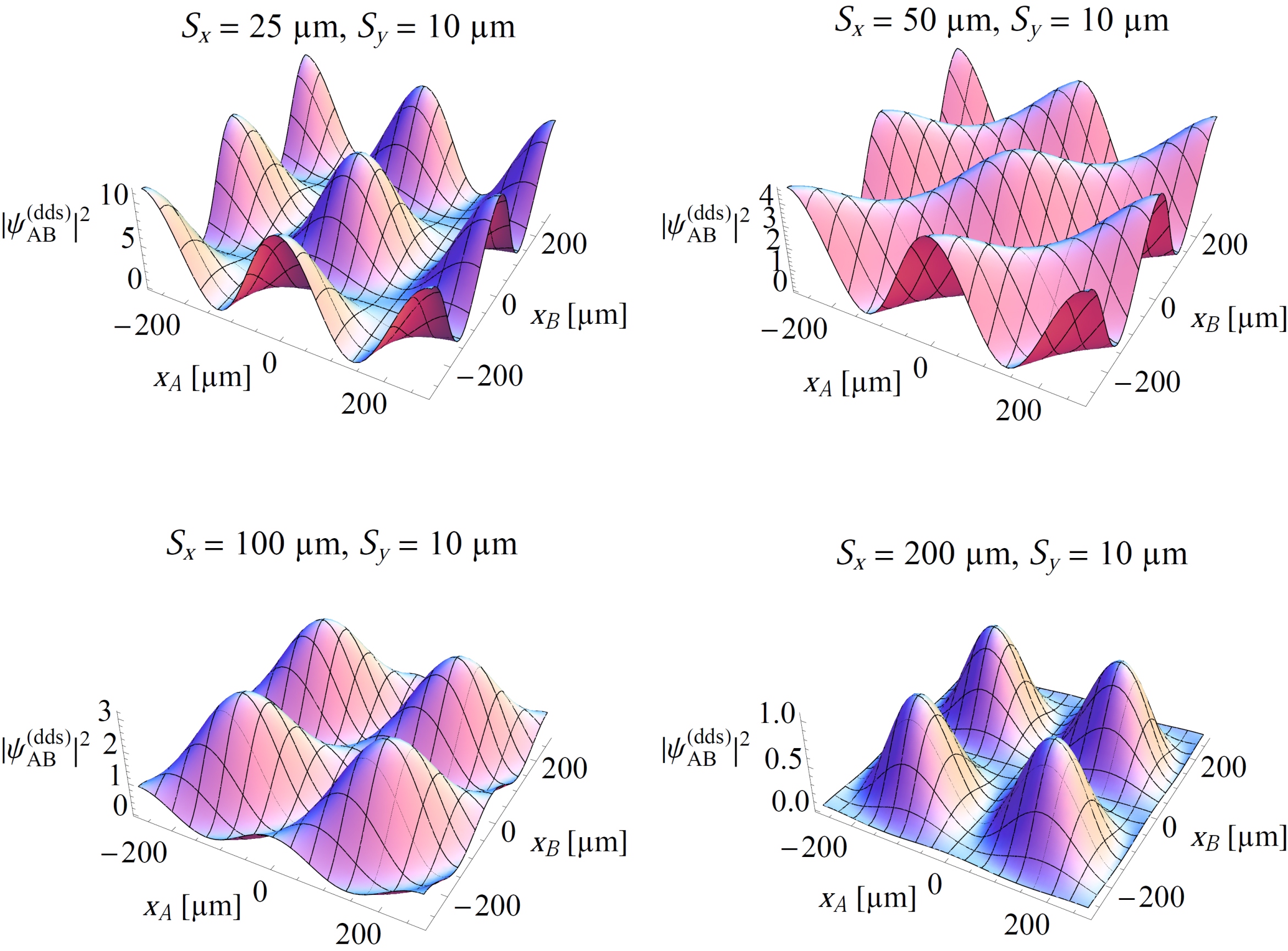
Figure 3: (Color online.) Two-particle probability distribution $|\psi_{\text{AB}}^{\text{(dds)}}|^{2}$ for the double double-slit experiment for different source sizes. The slit distance $d=100\,\mathrm{\SIUnitSymbolMicro}$m, source-slit distance $L_{1}=5\,$mm, and slit-detector distance $L_{2}=25\,$mm, are kept fixed, resulting in a constant fringe distance $d_{f}\simeq 271\,\mathrm{\SIUnitSymbolMicro}$m. For a very small source (top left, $S_{x}=25\,\mathrm{\SIUnitSymbolMicro}$m) the momentum spread of each individual particle is large and one obtains a product of two one-particle patterns of the form $\cos^{2}(\pi\tfrac{x_{\text{A}}}{d_{f}})\cos^{2}(\pi\tfrac{x_{\text{B}}}{d_{f}})$. If the source is larger than the slit distance (bottom right, $S_{x}=200\,\mathrm{\SIUnitSymbolMicro}$m), two two-particle patterns together wash out again into a factorizable pattern. An intermediate source size (top right, $S_{x}=50\,\mathrm{\SIUnitSymbolMicro}$m) fulfills all conditions for two-particle interference and shows a distribution of the unfactorizable form $\cos^{2}(\pi\tfrac{x_{\text{A}}-x_{\text{B}}}{d_{f}})$.

Figure 3 shows $|\psi_{\text{AB}}^{\text{(dds)}}|^{2}$ for various source sizes $S_{x}$. (The integration was done over a two-dimensional rectangular source with size $S_{y}=10\,$ µm along $y$ and constant weighting function. Integration over $y$ only marginally changes the pattern and so would an integration along $z$.) While in the top left picture ($S_{x}=25\,\mathrm{\SIUnitSymbolMicro}$m) condition (I) is violated, the bottom pictures ($S_{x}=100\,\mathrm{\SIUnitSymbolMicro}$m and $S_{x}=200\,\mathrm{\SIUnitSymbolMicro}$m) violate condition (III). The top right case ($S_{x}=50\,$ µm) shows a conditional interference pattern with high genuine two-particle visibility. For this choice of parameters conditions (8) read $28\,\mathrm{\SIUnitSymbolMicro}$m$\;\ll\;50\,\mathrm{\SIUnitSymbolMicro}$m$\;\ll\;100\,\mathrm{\SIUnitSymbolMicro}$m$\;<\;90\,\mathrm{\SIUnitSymbolMicro}$m and are approximately fulfilled. Decreasing or increasing the source size just a bit, lets us run into one or the other limitation. This shows that there is essentially no further freedom in any of the parameters given typical experimental constraints (falling height $H$, detector resolution $\delta x$). A double double-slit experiment therefore requires careful adjustment of the experimental parameters.

.3 III. Ghost interference

However, it turns out that we can circumvent condition (III), Ineq. (7), by removing one of the double-slits and using a ghost interference setup Stre1995 , as shown in Figure 4.

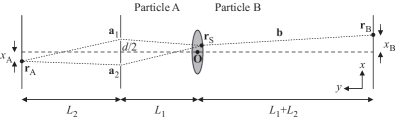
Figure 4: Schematic of the ghost interference experiment (top view, not drawn to scale). Pairs of atoms, A and B, are emitted from source points $\mathbf{r}_{\text{S}}$ within the BEC and arrive at detectors at positions $\mathbf{r}_{\text{A}}$ and $\mathbf{r}_{\text{B}}$. Only atom A passes through a double slit. See main text for details.

The possible path lengths from $\mathbf{r}_{\text{S}}$ to $\mathbf{r}_{\text{A}}\equiv(x_{\text{A}},L_{1}+L_{2},0)$ and $\mathbf{r}_{\text{B}}\equiv(x_{\text{B}},-L_{1}-L_{2},0)$ are abbreviated as $L_{\mathbf{a}_{i}}\equiv\overline{\mathbf{r}_{\text{S}}\mathbf{a}_{i}}+\overline{\mathbf{a}_{i}\mathbf{r}_{\text{A}}}$ ($i=1,2$) and $L_{\mathbf{b}}\equiv\overline{\mathbf{r}_{\text{S}}\mathbf{r}_{\text{B}}}$. The quantum mechanical amplitude for two entangled particles in ghost interference (gh), emerging from point $\mathbf{r}_{\text{S}}$, to land at points $\mathbf{r}_{\text{A}}$ and $\mathbf{r}_{\text{B}}$ is

$$\psi_{\text{SAB}}^{\text{(gh)}}(\mathbf{r}_{\text{S}},\mathbf{r}_{\text{A}},\mathbf{r}_{\text{B}})\propto\text{e}^{\text{i\thinspace}\frac{2\pi}{\lambda_{\text{dB}}}\,(L_{\mathbf{a}_{1}}+L_{\mathbf{b}})}+\text{e}^{\text{i\thinspace}\frac{2\pi}{\lambda_{\text{dB}}}\,(L_{\mathbf{a}_{2}}+L_{\mathbf{b}})}.$$ (9)

The quantum mechanical amplitude for two entangled particles, emerging from the whole source, to land at points $\mathbf{r}_{\text{A}}$ and $\mathbf{r}_{\text{B}}$ is again given by integration over all point sources:

$$\psi_{\text{AB}}^{\text{(gh)}}(\mathbf{r}_{\text{A}},\mathbf{r}_{\text{B}})\propto\dfrac{1}{V}\,{\displaystyle\iiint\nolimits_{\text{S}}}\,\text{d}\mathbf{r}_{\text{S}}\,g(\mathbf{r}_{\text{S}})\,\psi_{\text{SAB}}^{\text{(gh)}}(\mathbf{r}_{\text{S}},\mathbf{r}_{\text{A}},\mathbf{r}_{\text{B}}).$$ (10)

In the ghost interference setup with only one double-slit, condition (III) is not necessary any longer. The remaining conditions (I) and (II) in (8) can be easily fulfilled. Let us for instance choose $d=50\,\mathrm{\SIUnitSymbolMicro}$m, $L_{1}=5\,$mm, $L_{2}=25\,$mm. Due to the smaller slit distance as compared to the double double-slit scenario, the fringe distance on side A becomes $d_{f}^{\text{(A)}}=\lambda_{\text{dB}}\,\tfrac{L_{2}}{d}\simeq 542\,\mathrm{\SIUnitSymbolMicro}$m. The fringe distance on side B can be calculated via elementary geometrical considerations. It is $d_{f}^{\text{(B)}}=\lambda_{\text{dB}}\,\tfrac{2\,L_{1}+L_{2}}{d}\simeq 758\,\mathrm{\SIUnitSymbolMicro}$m. Both can easily be resolved with modern detectors. Conditions (I) and (II) read $S_{x}\gg 56\,\mathrm{\SIUnitSymbolMicro}$m, $d=50\,\mathrm{\SIUnitSymbolMicro}$m$\;\ll 83\,\mathrm{\SIUnitSymbolMicro}$m, leaving the only constraint $S_{x}\gg 56\,$ µm.

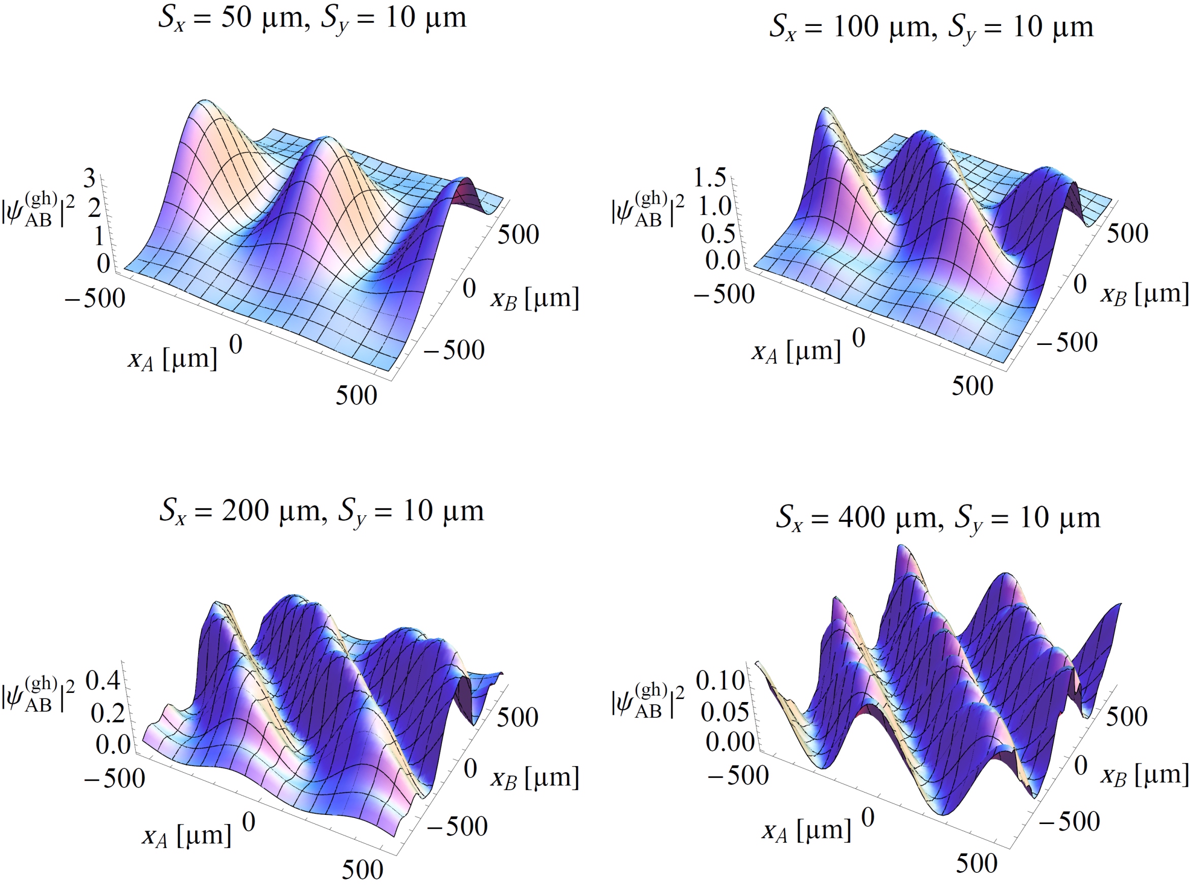
Figure 5: (Color online.) Two-particle probability distribution $|\psi_{\text{AB}}^{\text{(gh)}}|^{2}$ for the ghost interference experiment for different source sizes. The source-slit distance $L_{1}=5\,$mm and slit-detector distance $L_{2}=25\,$mm are the same as in Figure 3. The slit distance $d=50\,\mathrm{\SIUnitSymbolMicro}$m is smaller now, leading to larger fringe distances $d_{f}^{\text{(A)}}\simeq 542\,\mathrm{\SIUnitSymbolMicro}$m and $d_{f}^{\text{(B)}}\simeq 758\,\mathrm{\SIUnitSymbolMicro}$m at side A and B, respectively. A very small source (top left, $S_{x}=50\,\mathrm{\SIUnitSymbolMicro}$m) results in a product of two one-particle patterns. Large sources (bottom, $S_{x}=200\,\mathrm{\SIUnitSymbolMicro}$m and $400\,\mathrm{\SIUnitSymbolMicro}$m) show two-particle interference and produce a pattern of the unfactorizable form $\cos^{2}(\pi\tfrac{x_{\text{A}}+x_{\text{B}}}{d_{f}})$.

Figure 5 shows $|\psi_{\text{AB}}^{\text{(gh)}}|^{2}$ for different source sizes. One can see the transition from one-particle interference ($S_{x}=50\,$ µm, condition (I) not fulfilled) to almost perfect two-particle interference ($S_{x}=400\,$ µm) of the form $\cos^{2}(\pi\tfrac{x_{\text{A}}+x_{\text{B}}}{d_{f}})$. Note that condition (III), $S_{x}\ll d$, is clearly violated for the larger source sizes. Moreover, in contrast to the double double-slit experiment, the maximum of the interference pattern on one side is opposite to the conditioning detection on the other side.

Recently it was reported in Ref. Kher2012 that matter waves from colliding BECs violate the Cauchy-Schwarz inequality, ruling out a description in terms of classical stochastic random variable theories. The two-particle patterns discussed in the present work cannot be explained by classical correlations as soon as the two-particle visibility exceeds $\frac{1}{2}$ Ghos1987 ; Beli1992 . A strict proof that they must arise due to quantum entanglement can be made by employing a separability criterion using modular variables Gnei2011 .

.4 IV. Pair identification

Finally, we come to an important issue, namely the problem of identifying coincidences. The pulse duration of the lasers is of the order of 500 ns, which is negligible. The traveling time of the recoiled atoms from one side of the condensate to the center, i.e. a distance of about $100\,\mathrm{\SIUnitSymbolMicro}$m (more, if the condensate size is increased), is 1 ms. Therefore, all collisions certainly happen within $\Delta\tau_{\text{coll}}\simeq 1\,$ms, most of them likely within a fraction of that time. Ref. Perr2007 states that the time constant in the decay of the collision rate is $150\,$ µs. As discussed above, let us consider a pair of particles which collide into the $+y$ and $-y$ direction, with unchanged velocity component $v_{\text{rec}}$ along $+z$. Due to the velocity uncertainty we should assume that one particle has a velocity along $z$ of $v_{\text{rec}}$ and its entangled partner has $v_{\text{rec}}+\Delta v_{z}$. The times when they hit the detector plate are $\tau_{v_{\text{rec}}}\simeq 328.8\,$ms and $\tau_{v_{\text{rec}}+\Delta v_{z}}\simeq 329.7\,$ms. This means that two particles which must experimentally be identified as a coincidence can have a time spread of $\Delta\tau_{\text{pair}}\simeq 0.9\,$ms, which is of the order of the collision time scale $\Delta\tau_{\text{coll}}$. Two-particle interference requires to measure coincidences of entangled partners, i.e. identification of the correct subensemble on side A conditional on detection on side B. Since an identification by arrival time seems to be impossible, it appears to be necessary to reduce the laser intensity such that per shot, on average, only a few pairs collide in a way that they can reach the maximal lateral distance $L_{1}+L_{2}$ on opposite sides of the detector. Taking into account the finite detection efficiency makes the pair identification experimentally extremely challenging. It may be advantageous to replace the double slit (in ghost interference) by a grating to increase the possible count rates.

.5 V. Conclusion

An experimental demonstration of the original EPR gedanken experiment using momentum entanglement between pairs of two colliding BECs is within reach. While the problem of pair identification is very challenging, the constraints of source size, time-of-flight distances, and detector resolution are manageable and let conditional two-particle interference in a double double-slit configuration or a ghost interference setup seem feasible.

.6 Acknowledgments

The research was funded by the Doctoral Program CoQuS (Grant W1210) and SFB-FoQuS of the Austrian Science Fund (FWF).

References

- (1) A. Einstein, B. Podolsky, and N. Rosen, Phys. Rev. 47, 777 (1935).
- (2) E. Schrödinger, Naturwissenschaften 23, 807, 823, 844 (1935).
- (3) J. S. Bell, Physics (Long Island City, NY) 1, 195 (1964).
- (4) S. J. Freedman and J. F. Clauser, Phys. Rev. Lett. 28, 938 (1972).
- (5) A. Aspect, J. Dalibard, and G. Roger, Phys. Rev. Lett. 49, 1804 (1982).
- (6) P. G. Kwiat, K. Mattle, H. Weinfurter, A. Zeilinger, A. V. Sergienko, and Y. Shih, Phys. Rev. Lett. 75, 4337 (1995).
- (7) E. Hagley, X. Maître, G. Nogues, C. Wunderlich, M. Brune, J. M. Raimond, and S. Haroche, Phys. Rev. Lett. 79, 1 (1997).
- (8) C. Gross, H. Strobel, E. Nicklas, T. Zibold, N. Bar-Gill, G. Kurizik, M. K. Oberthaler, Nature. 480, 219 (2011).
- (9) Q. A. Turchette, C. S. Wood, B. E. King, C. J. Myatt, D. Leibfried, W. M. Itano, C. Monroe, and D. J. Wineland, Phys. Rev. Lett. 81, 3631 (1998).
- (10) M. A. Rowe, D. Kielpinski, V. Meyer, C. A. Sackett, W. M. Itano, C. Monroe, D. J. Wineland, Nature 409, 791 (2001).
- (11) M. Steffen, M. Ansmann, R. C. Bialczak, N. Katz, E. Lucero, R. McDermott, M. Neeley, E. M. Weig, A. N. Cleland, J. M. Martinis, Science 313, 1423 (2006).
- (12) Z. Y. Ou, S. F. Pereira, H. J. Kimble, and K. C. Peng, Phys. Rev. Lett. 68, 3663 (1992).
- (13) A. Perrin, H. Chang, V. Krachmalnicoff, M. Schellekens, D. Boiron, A. Aspect, and C. I. Westbrook, Phys. Rev. Lett. 99, 150405 (2007).
- (14) K. Mølmer, A. Perrin, V. Krachmalnicoff, V. Leung, D. Boiron, A. Aspect, and C. I. Westbrook, Phys. Rev. A 77, 033601 (2008).
- (15) A. Perrin, C. M. Savage, D. Boiron, V. Krachmalnicoff, C. I. Westbrook, and K. V. Kheruntsyan, New. J. Phys. 10, 045021 (2008).
- (16) M. A. Horne and A. Zeilinger, A possible spin-less experimental test of Bell’s inequality, in: Microphysical Reality and Quantum Formalism, edited by A. van der Merwe, F. Selleri, and G. Tarozzi (Kluwer Academic Publishers, 1988).
- (17) D. Greenberger, M. A. Horne, and A. Zeilinger, Phys. Today 46, 22 (1993).
- (18) M. A. Horne, Two-particle diffraction, in: Experimental Metaphysics, edited by R. S. Cohen, M. Horne, and J. Stachel (Kluwer Academic Publishers, 1997).
- (19) G. Jaeger, M. A. Horne, and A. Shimony, Phys. Rev. A 48, 1023 (1993).
- (20) J. Stenger, S. Inouye, A. P. Chikkatur, D. M. Stamper-Kurn, D. E. Pritchard, and W. Ketterle, Phys. Rev. Lett. 82, 4569 (1999).
- (21) D. V. Strekalov, A. V. Sergienko, D. N. Klyshko, and Y. H. Shih, Phys. Rev. Lett. 74, 3600 (1995).
- (22) K. V. Kheruntsyan, J.-C. Jaskula, P. Deuar, M. Bonneau, G. B. Patridge, J. Ruaudel, R. Lopes, D. Boiron, and C. I. Westbrook, Phys. Rev. Lett. 108, 260401 (2012).
- (23) C. Gneiting and K. Hornberger, Phys. Rev. Lett. 106, 210501 (2011).
- (24) R. Ghosh and L. Mandel, Phys. Rev. Lett. 59, 1903 (1987).
- (25) A. V. Belinsky and D. N. Klyshko, Phys. Lett. A 166, 303 (1992).