Lectures on Self-Avoiding Walks

Abstract.

These lecture notes provide a rapid introduction to a number of rigorous results on self-avoiding walks, with emphasis on the critical behaviour. Following an introductory overview of the central problems, an account is given of the Hammersley–Welsh bound on the number of self-avoiding walks and its consequences for the growth rates of bridges and self-avoiding polygons. A detailed proof that the connective constant on the hexagonal lattice equals $\sqrt{2+\sqrt{2}}$ is then provided. The lace expansion for self-avoiding walks is described, and its use in understanding the critical behaviour in dimensions $d>4$ is discussed. Functional integral representations of the self-avoiding walk model are discussed and developed, and their use in a renormalisation group analysis in dimension $4$ is sketched. Problems and solutions from tutorials are included.

Foreword

These notes are based on a course on Self-Avoiding Walks given in Búzios, Brazil, in August 2010, as part of the Clay Mathematics Institute Summer School and the XIV Brazilian Probability School. The course consisted of six lectures by Gordon Slade, a lecture by Hugo Duminil-Copin based on recent joint work with Stanislav Smirnov (see Section 3), and tutorials by Roland Bauerschmidt and Jesse Goodman. The written version of Slade’s lectures was drafted by Bauerschmidt and Goodman, and the written version of Duminil-Copin’s lecture was drafted by himself. The final manuscript was integrated and prepared jointly by the four authors.

1. Introduction and overview of the critical behaviour

These lecture notes focus on a number of rigorous results for self-avoiding walks on the $d$-dimensional integer lattice ${\mathbb{Z}}^{d}$. The model is defined by assigning equal probability to all paths of length $n$ starting from the origin and without self-intersections. This family of probability measures is not consistent as $n$ is varied, and thus does not define a stochastic process; the model is combinatorial in nature. The natural questions about self-avoiding walks concern the asymptotic behaviour as the length of the paths tends to infinity. Despite its simple definition, the self-avoiding walk is difficult to study in a mathematically rigorous manner. Many of the important problems remain unsolved, and the basic problems encompass many of the features and challenges of critical phenomena. This section gives the basic definitions and an overview of the critical behaviour.

1.1. Simple random walks

The basic reference model is simple random walk (SRW). Let $\Omega\subset\mathbb{Z}^{d}$ be the set of possible steps. The primary examples considered in these lectures are

(1.1) $$\begin{split}\text{the nearest-neighbour model:}\qquad\quad\Omega&=\left\{x\in\mathbb{Z}^{d}:\left\lVert x\right\rVert_{1}=1\right\},\\ \text{the spread-out model:}\qquad\quad\Omega&=\left\{x\in\mathbb{Z}^{d}:0<\left\lVert x\right\rVert_{\infty}\leq L\right\},\end{split}$$

where $L$ is a fixed integer, usually large. An $n$-step walk is a sequence $\omega=(\omega(0),\omega(1),\dotsc,\omega(n))$ with $\omega(j)-\omega(j-1)\in\Omega$ for $j=1,\dotsc,n$. The $n$-step simple random walk is the uniform measure on $n$-step walks. We define the sets

(1.2) $$\mathcal{W}_{n}(0,x)=\{\omega:\omega\text{ is an $n$-step walk with $\omega(0)=0$ and $\omega(n)=x$}\}$$

and

(1.3) $$\mathcal{W}_{n}=\bigcup_{x\in\mathbb{Z}^{d}}\mathcal{W}_{n}(0,x).$$

1.2. Self-avoiding walks

The weakly self-avoiding walk and the strictly self-avoiding walk (the latter also called simply self-avoiding walk) are the main subjects of these notes. These are random paths on $\mathbb{Z}^{d}$, defined as follows. Given an $n$-step walk $\omega\in\mathcal{W}_{n}$, and integers $s,t$ with $0\leq s<t\leq n$, let

(1.4) $$U_{st}=U_{st}(\omega)=-1_{\left\{\omega(s)=\omega(t)\right\}}=\begin{cases}-1&\text{if $\omega(s)=\omega(t)$},\\ \;\;\,0&\text{if $\omega(s)\neq\omega(t)$}.\end{cases}$$

Fix $\lambda\in[0,1]$. We assign to each path $\omega\in\mathcal{W}_{n}$ the weighting factor

(1.5) $$\prod_{0\leq s<t\leq n}(1+\lambda U_{st}(\omega)).$$

The weights can also be expressed as Boltzmann weights:

(1.6) $$\prod_{0\leq s<t\leq n}(1+\lambda U_{st}(\omega))=\exp\Bigl{(}-g\sum_{0\leq s<t\leq n}1_{\left\{\omega(s)=\omega(t)\right\}}\Bigr{)}$$

with $g=-\log(1-\lambda)\in[0,\infty)$ for $\lambda\in[0,1)$. Making the convention $\infty\cdot 0=0$, the case $\lambda=1$ corresponds to $g=\infty$.

The choice $\lambda=0$ assigns equal weight to all walks in $\mathcal{W}_{n}$; this is the case of the simple random walk. For $\lambda\in(0,1)$, self-intersections are penalised but not forbidden, and the model is called the weakly self-avoiding walk. The choice $\lambda=1$ prevents any return to a previously visited site, and defines the self-avoiding walk (SAW). More precisely, an $n$-step walk $\omega$ is a self-avoiding walk if and only if the expression (1.5) is non-zero for $\lambda=1$, which happens if and only if $\omega$ visits each site at most once, and for such walks the weight equals $1$.

These weights give rise to associated partition sums $c_{n}^{(\lambda)}(x)$ and $c_{n}^{(\lambda)}$ for walks in $\mathcal{W}_{n}(0,x)$ and $\mathcal{W}_{n}$, respectively:

(1.7) $$c_{n}^{(\lambda)}(x)=\sum_{\omega\in\mathcal{W}_{n}(0,x)}\prod_{0\leq s<t\leq n}(1+\lambda U_{st}(\omega)),\quad c_{n}^{(\lambda)}=\sum_{x\in\mathbb{Z}^{d}}c_{n}^{(\lambda)}(x).$$

In the case $\lambda=1$, $c_{n}^{(1)}(x)$ counts the number of self-avoiding walks of length $n$ ending at $x$, and $c_{n}^{(1)}$ counts all $n$-step self-avoiding walks. The case $\lambda=0$ reverts to simple random walk, for which $c_{n}^{(0)}=\left\lvert\Omega\right\rvert^{n}$. When $\lambda=1$ we will often drop the superscript $(1)$ and write simple $c_{n}$ instead of $c_{n}^{(1)}$.

We also define probability measures $\mathbb{Q}^{(\lambda)}_{n}$ on $\mathcal{W}_{n}$ with expectations $\mathbb{E}^{(\lambda)}_{n}$:

(1.8) $$\mathbb{Q}_{n}^{(\lambda)}(A)=\frac{1}{c_{n}^{(\lambda)}}\sum_{\omega\in A}\prod_{0\leq s<t\leq n}(1+\lambda U_{st}(\omega))\quad(A\subset\mathcal{W}_{n}),$$

(1.9) $$\mathbb{E}_{n}^{(\lambda)}(X)=\frac{1}{c_{n}^{(\lambda)}}\sum_{\omega\in\mathcal{W}_{n}}X(\omega)\prod_{0\leq s<t\leq n}(1+\lambda U_{st}(\omega))\quad(X:\mathcal{W}_{n}\to{\mathbb{R}}).$$

The measures $\mathbb{Q}_{n}^{(\lambda)}$ define the weakly self-avoiding walk when $\lambda\in(0,1)$ and the strictly self-avoiding walk when $\lambda=1$. Occasionally we will also consider self-avoiding walks that do not begin at the origin.

1.3. Subadditivity and the connective constant

The sequence $c_{n}^{(\lambda)}$ has the following submultiplicativity property:

(1.10) $$c_{n+m}^{(\lambda)}\leq\sum_{\omega\in\mathcal{W}_{n+m}}\prod_{0\leq s<t\leq n}(1+\lambda U_{st})\prod_{n\leq s^{\prime}<t^{\prime}\leq n+m}(1+\lambda U_{s^{\prime}t^{\prime}})\leq c_{n}^{(\lambda)}c_{m}^{(\lambda)}.$$

Therefore, $\log c_{n}^{(\lambda)}$ is a subadditive sequence: $\log c_{n+m}^{(\lambda)}\leq\log c_{n}^{(\lambda)}+\log c_{m}^{(\lambda)}$.

Lemma 1.1.

If $a_{1},a_{2},\dotsc\in\mathbb{R}$ obey $a_{n+m}\leq a_{n}+a_{m}$ for every $n,m$, then

(1.11) $$\lim_{n\to\infty}\frac{a_{n}}{n}=\inf_{n\geq 1}\frac{a_{n}}{n}\in[-\infty,\infty).$$

Proof.

See Problem 1.1. The value $-\infty$ is possible, e.g., for the sequence $a_{n}=-n^{2}$. ∎

Applying Lemma 1.1 to $c_{n}^{(\lambda)}$ gives the existence of $\mu_{\lambda}$ such that $\lim\frac{1}{n}\log c_{n}^{(\lambda)}=\log\mu_{\lambda}\leq\frac{1}{n}\log c_{n}^{(\lambda)}$ for all $n$, i.e.,

(1.12) $$\mu_{\lambda}=\lim_{n\to\infty}(c_{n}^{(\lambda)})^{1/n}\text{ exists, and}\quad c_{n}^{(\lambda)}\geq\mu_{\lambda}^{n}\quad\text{for all $n$}.$$

In the special case $\lambda=1$, we write simply $\mu=\mu_{1}$. This $\mu$, which depends on $d$ (and also on $L$ for the spread-out model), is called the connective constant. For the nearest-neighbour model, by counting only walks that move in positive coordinate directions, and by counting walks that are restricted only to prevent immediate reversals of steps, we obtain

(1.13) $$d^{n}\leq c_{n}\leq 2d(2d-1)^{n-1}\qquad\text{which implies}\qquad d\leq\mu\leq 2d-1.$$

For $d=2$, the following rigorous bounds are known:

(1.14) $$\mu\in[2.625\,622,2.679\,193].$$

The lower bound is due to Jensen [47] via bridge enumeration (bridges are defined in Section 2.1 below), and the upper bound is due to Pönitz and Tittmann [64] by comparison with finite-memory walks. The estimate

(1.15) $$\mu=2.638\,158\,530\,31(3)$$

is given in [45]; here the $3$ in parentheses represents the subjective error in the last digit. It has been observed that $1/\mu$ is well approximated by the smallest positive root of $581x^{4}+7x^{2}-13=0$ [23, 48], though no derivation or explanation of this quartic polynomial is known, and later evidence has raised doubts about its validity [45].

Even though the definition of self-avoiding walks has been restricted to the graph $\mathbb{Z}^{d}$ thus far, it applies more generally. In 1982, arguments based on a Coulomb gas formalism led Nienhuis [61] to predict that on the hexagonal lattice the connective constant is equal to $\sqrt{2+\sqrt{2}}$. This was very recently proved by Duminil-Copin and Smirnov [24], whose theorem is the following.

Theorem 1.2.

The connective constant for the hexagonal lattice is

(1.16) $$\mu=\textstyle{\sqrt{2+\sqrt{2}}}.$$

The proof of Theorem 1.2 is presented in Section 3 below. Except for trivial cases, this is the only lattice for which the connective constant is known explicitly.

Returning to ${\mathbb{Z}}^{d}$, in 1963, Kesten [50] proved that

(1.17) $$\lim_{n\to\infty}\frac{c_{n+2}}{c_{n}}=\mu^{2},$$

but it remains an open problem (for $d=2,3,4$) to prove that

(1.18) $$\lim\limits_{n\to\infty}\dfrac{c_{n+1}}{c_{n}}=\mu.$$

Even the proof of $c_{n+1}\geq c_{n}$ is a non-trivial result, proved by O’Brien [62], though it is not hard to show that $c_{n+2}\geq c_{n}$.

1.4. $1/d$ expansion

It was proved by Hara and Slade [35] that the connective constant $\mu(d)$ for $\mathbb{Z}^{d}$ (with nearest-neighbour steps) has an asymptotic expansion in powers of $1/2d$ as $d\to\infty$: There exist integers $a_{i}\in\mathbb{Z}$, $i=-1,0,1,\dotsc$ such that

(1.19) $$\mu(d)\sim\sum_{i=-1}^{\infty}\frac{a_{i}}{(2d)^{i}}$$

in the sense that $\mu(d)=a_{-1}(2d)+a_{0}+\dotsb+a_{M-1}(2d)^{-(M-1)}+O(d^{-M})$, for each fixed $M$. In Problem 5.1 below, the first three terms are computed. The constant in the $O(d^{-M})$ term may depend on $M$. It is expected, though not proved, that the asymptotic series in (1.19) has radius of convergence $0$, so that the right-hand side of (1.19) diverges for each fixed $d$. The values of $a_{i}$ are known for $i=-1,0,\dotsc,11$ and grow rapidly in magnitude; see Clisby, Liang, and Slade [21].

Graham [26] has proved Borel-type error bounds for the asymptotic expansion of $z_{c}=z_{c}(d)=\mu^{-1}$. Namely, writing the asymptotic expansion of $z_{c}$ as $\sum_{i=1}^{\infty}\alpha_{i}(2d)^{-i}$, there is a constant $C$, independent of $d$ and $M$, such that for each $M$ and for all $d\geq 1$,

(1.20) $$\Big{|}z_{c}-\sum_{i=1}^{M-1}\frac{\alpha_{i}}{(2d)^{i}}\Big{|}\leq\frac{C^{M}M!}{(2d)^{M}}.$$

An extension of (1.20) to complex values of the dimension $d$ would be needed in order to apply the method of Borel summation to recover the value of $z_{c}$, and hence of $\mu(d)$, from the asymptotic series.

1.5. Critical exponents

It is a characteristic feature of models of statistical mechanics at the critical point that there exist critical exponents which describe the asymptotic behaviour on the large scale. It is a deep conjecture, not yet properly understood mathematically, that these critical exponents are universal, meaning that they depend only on the spatial dimension of the system, but not on details such as the specific lattice in $\mathbb{R}^{d}$. For the case of the self-avoiding walk, this conjecture of universality extends to lack of dependence on the constant $\lambda$, as soon as $\lambda>0$. We now introduce the critical exponents, and in Section 1.6 we will discuss what is known about them in more detail.

1.5.1. Number of self-avoiding walks

It is predicted that for each $d$ there is a constant $\gamma$ such that for all $\lambda\in(0,1]$, and for both the nearest-neighbour and spread-out models,

(1.21) $$c_{n}^{(\lambda)}\sim A_{\lambda}\mu_{\lambda}^{n}n^{\gamma-1}.$$

Here $f(n)\sim g(n)$ means $\lim_{n\to\infty}f(n)/g(n)=1$. The predicted values of the critical exponent $\gamma$ are:

(1.22) $$\gamma=\begin{cases}1&d=1,\\ \tfrac{43}{32}&d=2,\\ 1.16\ldots&d=3,\\ 1&d=4,\\ 1&d\geq 5.\end{cases}$$

In fact, for $d=4$, the prediction involves a logarithmic correction:

(1.23) $$c_{n}^{(\lambda)}\sim A_{\lambda}\mu_{\lambda}^{n}(\log n)^{1/4}.$$

This situation should be compared with simple random walk, for which $c_{n}^{(0)}=\left\lvert\Omega\right\rvert^{n}$, so that $\mu_{0}$ is equal to the degree $\left\lvert\Omega\right\rvert$ of the lattice, and $\gamma=1$.

In the case of the self-avoiding walk (i.e., $\lambda=1$), $\gamma$ has a probabilistic interpretation. Sampling independently from two $n$-step self-avoiding walks uniformly,

(1.24) $$\mathbb{P}(\omega_{1}\cap\omega_{2}=\left\{0\right\})=\frac{c_{2n}}{c_{n}^{2}}\sim{\rm const}\frac{1}{n^{\gamma-1}},$$

so $\gamma$ is a measure of how likely it is for two self-avoiding walks to avoid each other. The analogous question for SRW is discussed in [53].

Despite the precision of the prediction (1.21), the best rigorously known bounds in dimension $d=2,3,4$ are very far from tight and almost 50 years old. In [29], Hammersley and Welsh proved that, for all $d\geq 2$,

(1.25) $$\mu^{n}\leq c_{n}\leq\mu^{n}e^{\kappa\sqrt{n}}$$

(the lower bound is just subadditivity, the upper bound is nontrivial). This was improved slightly by Kesten [50], who showed that for $d=3,4,\ldots$,

(1.26) $$\mu^{n}\leq c_{n}\leq\mu^{n}\exp\left(\kappa n^{2/(d+2)}\log n\right).$$

The proof of the Hammersley–Welsh bound is the subject of Section 2.1.

1.5.2. Mean-square displacement

Let $|x|$ denote the Euclidean norm of $x\in\mathbb{R}^{d}$. It is predicted that for $\lambda\in(0,1]$, and for both the nearest-neighbour and spread-out models,

(1.27) $$\mathbb{E}_{n}^{(\lambda)}\left\lvert\omega(n)\right\rvert^{2}\sim D_{\lambda}n^{2\nu},$$

with

(1.28) $$\nu=\begin{cases}1&d=1,\\ \tfrac{3}{4}&d=2,\\ 0.588\ldots&d=3,\\ \tfrac{1}{2}&d=4,\\ \tfrac{1}{2}&d\geq 5.\end{cases}$$

Again, a logarithmic correction is predicted for $d=4$:

(1.29) $$\mathbb{E}_{n}^{(\lambda)}\left\lvert\omega(n)\right\rvert^{2}\sim D_{\lambda}n(\log n)^{1/4}.$$

This should be compared with the SRW, for which $\nu=\tfrac{1}{2}$ in all dimensions.

Almost nothing is known rigorously about $\nu$ in dimensions $2,3,4$. It is an open problem to show that the mean-square displacement grows at least as rapidly as simple random walk, and grows more slowly than ballistically, i.e., it has not been proved that

(1.30) $$cn\leq\mathbb{E}_{n}^{(1)}\left\lvert\omega(n)\right\rvert^{2}\leq Cn^{2-\epsilon},$$

or even that the endpoint is typically as far away as the surface of a ball of volume $n$, i.e., $cn^{2/d}\leq\mathbb{E}_{n}^{(1)}\left\lvert\omega(n)\right\rvert^{2}$. Madras (unpublished) has shown $\mathbb{E}_{n}^{(1)}\left\lvert\omega(n)\right\rvert^{2}\geq cn^{4/3d}$.

1.5.3. Two-point function and susceptibility

The two-point function is defined by

(1.31) $$G_{z}^{(\lambda)}(x)=\sum_{n=0}^{\infty}c_{n}^{(\lambda)}(x)z^{n},$$

and the susceptibility by

(1.32) $$\chi^{(\lambda)}(z)=\sum_{x\in\mathbb{Z}^{d}}G_{z}^{(\lambda)}(x)=\sum_{n=0}^{\infty}c_{n}^{(\lambda)}z^{n}.$$

Since $\chi^{(\lambda)}$ is a power series whose coefficients satisfy (1.12), its radius of convergence $z_{c}^{(\lambda)}$ is given by $z_{c}^{(\lambda)}=\mu_{\lambda}^{-1}$. The value $z_{c}^{(\lambda)}$ is referred to as the critical point.

Proposition 1.3.

Fix $\lambda\in[0,1],z\in(0,z_{c}^{(\lambda)})$. Then $G_{z}^{(\lambda)}(x)$ decays exponentially in $x$.

Proof.

For simplicity, we consider only the nearest-neighbour model, and we omit $\lambda$ from the notation. Since $c_{n}(x)=0$ if $n<\left\lVert x\right\rVert_{1}$,

(1.33) $$G_{z}(x)=\sum_{n=\left\lVert x\right\rVert_{1}}^{\infty}c_{n}(x)z^{n}\leq\sum_{n=\left\lVert x\right\rVert_{1}}^{\infty}c_{n}z^{n}.$$

Fix $z<z_{c}=1/\mu$ and choose $\epsilon>0$ such that $z(\mu+\epsilon)<1$. Since $c_{n}^{1/n}\to\mu$, there exists $K=K(\epsilon)$ such that $c_{n}\leq K(\mu+\epsilon)^{n}$ for all $n$. Hence

(1.34) $$G_{z}(x)\leq K\sum_{n=\left\lVert x\right\rVert_{1}}^{\infty}(z(\mu+\epsilon))^{n}\leq K^{\prime}(z(\mu+\epsilon))^{\left\lVert x\right\rVert_{1}},$$

as claimed. ∎

We restrict temporarily to $\lambda=1$. Much is known about $G_{z}(x)$ for $z<z_{c}$: there is a norm $\left\lvert\,\cdot\,\right\rvert_{z}$ on $\mathbb{R}^{d}$, satisfying $\|u\|_{\infty}\leq\left\lvert u\right\rvert_{z}\leq\|u\|_{1}$ for all $u\in\mathbb{R}^{d}$, such that $m(z)=\lim\limits_{\left\lvert x\right\rvert_{z}\to\infty}-\frac{\log G_{z}(x)}{\left\lvert x\right\rvert_{z}}$ exists and is finite. The correlation length is defined by $\xi(z)=1/m(z)$, and hence approximately

(1.35) $$G_{z}(x)\approx e^{-\left\lvert x\right\rvert_{z}/\xi(z)}.$$

Indeed, more precise asymptotics (Ornstein–Zernike decay) are known [17, 57, 15]:

(1.36) $$G_{z}(x)\sim\frac{c}{|x|_{z}^{(d-1)/2}}e^{-|x|_{z}/\xi(z)}\quad\text{as $x\to\infty$},$$

and the arguments leading to this also prove that

(1.37) $$\lim\limits_{z\nearrow z_{c}}\xi(z)=\infty.$$

As a refinement of (1.37), it is predicted that as $z\nearrow z_{c}$,

(1.38) $$\xi(z) \sim\mathrm{const}\left(1-\frac{z}{z_{c}}\right)^{-\nu},$$

and that, in addition, as $\left\lvert x\right\rvert\to\infty$ (for $d\geq 2$),

(1.39) $$G_{z_{c}}(x) \sim\frac{\mathrm{const}}{\left\lvert x\right\rvert^{d-2+\eta}}.$$

The exponents $\gamma$, $\eta$ and $\nu$ are predicted to be related to each other via Fisher’s relation (see, e.g., [57]):

(1.40) $$\gamma=(2-\eta)\nu.$$

There is typically a correspondence between the asymptotic growth of the coefficients in a generating function and the behaviour of the generating function near its dominant singularity. For our purpose we note that, under suitable hypotheses,

(1.41) $$a_{n}\sim\frac{n^{\gamma-1}}{R^{n}}\text{ as $n\to\infty$}\qquad\overset{\approx}{\Longleftrightarrow}\qquad\sum_{n}a_{n}z^{n}\sim\frac{C}{(1-z/R)^{\gamma}}\text{ as $z\nearrow R$}.$$

The easier $\implies$ direction is known as an Abelian theorem, and the more delicate $\Longleftarrow$ direction is known as a Tauberian theorem [36]. With this in mind, our earlier prediction for $c_{n}^{(\lambda)}$ for $\lambda\in(0,1]$ corresponds to:

(1.42) $$\chi^{(\lambda)}(z)\sim\frac{\mathrm{const}_{\lambda}}{(1-z/z_{c})^{\gamma}}$$

as $z\nearrow z_{c}$, with an additional factor $\left\lvert\log(1-z/z_{c})\right\rvert^{1/4}$ on the right-hand side when $d=4$.

1.6. Effect of the dimension

Universality asserts that self-avoiding walks on different lattices in a fixed dimension $d$ should behave in the same way, independently of the fine details of how the model is defined. However, the behaviour does depend very strongly on the dimension.

1.6.1. $d=1$

For the nearest-neighbour model with $\lambda=1$ it is a triviality that $c_{n}^{(1)}=2$ for all $n\geq 1$ and $\left\lvert\omega(n)\right\rvert=n$ for all $\omega$, since a self-avoiding walk must continue either in the negative or in the positive direction. Any configuration $\omega\in\mathcal{W}_{n}$ is possible when $\lambda\in(0,1)$, however, and it is by no means trivial to prove that the critical behaviour when $\lambda\in(0,1)$ is similar to the case of $\lambda=1$. The following theorem of König [52] (extending a result of Greven and den Hollander [27]) proves that the weakly self-avoiding walk measure (1.8) does have ballistic behaviour for all $\lambda\in(0,1)$.

Theorem 1.4.

Let $d=1$. For each $\lambda\in(0,1)$, there exist $\theta(\lambda)\in(0,1)$ and $\sigma(\lambda)\in(0,\infty)$ such that for all $u\in\mathbb{R}$,

(1.43) $$\lim_{n\to\infty}\mathbb{Q}_{n}^{(\lambda)}\!\left(\frac{\left\lvert\omega(n)\right\rvert-n\theta}{\sigma\sqrt{n}}\leq u\right)=\int_{-\infty}^{u}\frac{e^{-t^{2}/2}}{\sqrt{2\pi}}\,dt.$$

A similar result is proved in [52] for the 1-dimensional spread-out strictly self-avoiding walk. The result of Theorem 1.4 should be contrasted to the case $\lambda=0$, which has diffusive rather than ballistic behaviour. It remains an open problem to prove the intuitively appealing statement that $\theta$ should be an increasing function of $\lambda$. A review of results for $d=1$ is given in [40].

1.6.2. $d=2$

Based on non-rigorous Coulomb gas methods, Nienhuis [61] predicted that $\gamma=\tfrac{43}{32}$, $\nu=\tfrac{3}{4}$. These predicted values have been confirmed numerically by Monte Carlo simulation, e.g., [55], and exact enumeration of self-avoiding walks up to length $n=71$ [46].

Lawler, Schramm, and Werner [54] have given major mathematical support to these predictions. Roughly speaking, they show that if self-avoiding walk has a scaling limit, and if this scaling limit has a certain conformal invariance property, then the scaling limit must be $\mathrm{SLE}_{8/3}$ (the Schramm–Loewner evolution with parameter $\kappa=\frac{8}{3}$). The values of $\gamma$ and $\nu$ are then recovered from an $\mathrm{SLE}_{8/3}$ computation. Numerical evidence supporting the statement that the scaling limit is $\mathrm{SLE}_{8/3}$ is given in [49]. However, until now, it remains an open problem to prove the required existence and conformal invariance of the scaling limit.

The result of [54] is discussed in greater detail in the course of Vincent Beffara [1]. Here, we describe it only briefly, as follows. Consider a simply connected domain $\Omega$ in the complex plane $\mathbb{C}$ with two points $a$ and $b$ on the boundary. Fix $\delta>0$, and let $(\Omega_{\delta},a_{\delta},b_{\delta})$ be a discrete approximation of $(\Omega,a,b)$ in the following sense: $\Omega_{\delta}$ is the largest finite domain of $\delta\mathbb{Z}^{2}$ included in $\Omega$, $a_{\delta}$ and $b_{\delta}$ are the closest vertices of $\delta\mathbb{Z}^{2}$ to $a$ and $b$ respectively. When $\delta$ goes to 0, this provides an approximation of the domain.

For fixed $z,\delta>0$, there is a probability measure on the set of self-avoiding walks $\omega$ between $a_{\delta}$ and $b_{\delta}$ that remain in $\Omega_{\delta}$ by assigning to $\omega$ a Boltzmann weight proportional to $z^{\ell(\omega)}$, where $\ell(\omega)$ denotes the length of $\omega$. We obtain a random piecewise linear curve, denoted by $\omega_{\delta}$.

It is possible to prove that when $z<z_{c}=1/\mu$, walks are penalised so much with respect to their length that $\omega_{\delta}$ becomes straight when $\delta$ goes to 0; this is closely related to the Ornstein–Zernike decay results. On the other hand, it is expected that, when $z>z_{c}$, the entropy wins against the penalisation and $\omega_{\delta}$ becomes space filling when $\delta$ tends to 0. Finally, when $z=z_{c}$, the sequence of measures conjecturally converges to a random continuous curve. It is for this case that we have the following conjecture of Lawler, Schramm and Werner [54].

Conjecture 1.5.

For $z=z_{c}$, the random curve $\omega_{\delta}$ converges to $\mathrm{SLE}_{8/3}$ from $a$ and $b$ in the domain $\Omega$.

It remains a major open problem in 2-dimensional statistical mechanics to prove the conjecture.

1.6.3. $d=3$

For $d=3$, there are no rigorous results for critical exponents, and no mathematically well-defined candidate has been proposed for the scaling limit. An early prediction for the values of $\nu$, referred to as the Flory values [25], was $\nu=\frac{3}{d+2}$ for $1\leq d\leq 4$. This does give the correct answer for $d=1,2,4$, but it is not quite accurate for $d=3$—the Flory argument is very remote from a rigorous mathematical proof. Flory’s interest in the problem was motivated by the use of SAWs to model polymer molecules; this application is discussed in detail in the course of Frank den Hollander [42] (see also [43]).

For $d=3$, there are three methods to compute the exponents approximately. In one method, non-rigorous field theory computations in theoretical physics [28] combine the $n\to 0$ limit for the $O(n)$ model with an expansion in $\epsilon=4-d$ about dimension $d=4$, with $\epsilon=1$. Secondly, Monte Carlo studies have been carried out with walks of length 33,000,000 [20], using the pivot algorithm [58, 44]. Finally, exact enumeration plus series analysis has been used; currently the most extensive enumerations in dimensions $d\geq 3$ use the lace expansion [21], and for $d=3$ walks have been enumerated to length $n=30$. The exact enumeration estimates for $d=3$ are $\mu=4.684043(12)$, $\gamma=1.1568(8)$, $\nu=0.5876(5)$ [21]. Monte Carlo estimates are consistent with these values: $\gamma=1.1575(6)$ [16] and $\nu=0.587597(7)$ [20].

1.6.4. $d=4$

Four dimensions is the upper critical dimension for the self-avoiding walk. This term encapsulates the notion that for $d>4$ self-avoiding walk has the same critical behaviour as simple random walk, while for $d<4$ it does not. The dimension $4$ can be guessed by considering the fractal properties of the simple random walk: for $d\geq 2$, the path of a simple random walk is two-dimensional. If $d>4$, two independent two-dimensional objects should generically not intersect, so that the effect of self-interaction between the past and the future of a simple random walk should be negligible. In $d=4$, the expected number of intersections between two independent random walks tends to infinity, but only logarithmically in the length. Such considerations are related to the logarithmic corrections that appear in (1.23) and (1.29).

The existence of logarithmic corrections to scaling has been proved for models of weakly self-avoiding walk on a 4-dimensional hierarchical lattice, using rigorous renormalisation group methods [5, 9, 10, 32]. The hierarchical lattice is a simplification of the hypercubic lattice $\mathbb{Z}^{4}$ which is particularly amenable to the renormalisation group approach. Recently there has been progress in the application of renormalisation group methods to a continuous-time weakly self-avoiding walk model on $\mathbb{Z}^{4}$ itself, and in particular it has been proved in this context that the critical two-point function has $|x|^{-2}$ decay [12], which is a statement that the critical exponent $\eta$ is equal to $0$. This is the topic of Section 7 below.

1.6.5. $d\geq 5$

Using the lace expansion, it has been proved that for the nearest-neighbour model in dimensions $d\geq 5$ the critical exponents exist and take their so-called mean field values $\gamma=1$, $\nu=\frac{1}{2}$ [34, 33] and $\eta=0$ [30], and that the scaling limit is Brownian motion [33]. The lace expansion for self-avoiding walks is discussed in Section 4, and its application to prove simple random walk behaviour in dimensions $d\geq 5$ is discussed in Section 5.

1.7. Tutorial

Problem 1.1.

Let $(a_{n})$ be a real-valued sequence that is subadditive, that is, $a_{n+m}\leq a_{n}+a_{m}$ holds for all $n,m$. Prove that $\lim_{n\to\infty}n^{-1}a_{n}$ exists in $[-\infty,\infty)$ and equals $\inf_{n}n^{-1}a_{n}$.

Problem 1.2.

Prove that the connective constant $\mu$ for the nearest-neighbour model on the square lattice $\mathbb{Z}^{2}$ obeys the strict inequalities $2<\mu<3$.

Problem 1.3.

A family of probability measures $(\mathbb{P}_{n})$ on $\mathcal{W}_{n}$ is called consistent if $\mathbb{P}_{n}(\omega)=\sum_{\rho>\omega}\mathbb{P}_{m}(\rho)$ for all $m>n$ and for all $\omega\in\mathcal{W}_{n}$, where the sum is over all $\rho\in\mathcal{W}_{m}$ whose first $n$ steps agree with $\omega$. Show that $\mathbb{Q}_{n}^{(1)}$, the uniform measure on SAWs, does not provide a consistent family.

Problem 1.4.

Show that the Fourier transform of the two-point function of the 1-dimensional strictly self-avoiding walk is given by

(1.44) $$\hat{G}_{z}(k)=\frac{1-z^{2}}{1+z^{2}-2z\cos k}.$$

Here $\hat{f}(k)=\sum_{x\in\mathbb{Z}^{d}}f(x)e^{ik\cdot x}$.

Problem 1.5.

Suppose that $f(z)=\sum_{n=0}^{\infty}a_{n}z^{n}$ has radius of convergence $1$. Suppose that $|f(z)|\leq c|1-z|^{-b}$ uniformly in $|z|<1$, with $b\geq 1$. Prove that, for some constant $C$, $|a_{n}|\leq Cn^{b-1}$ if $b>1$, and that $|a_{n}|\leq C\log n$ if $b=1$. Hint:

(1.45) $$a_{n}=\frac{1}{2\pi i}\oint_{\Gamma_{n}}\frac{f(z)}{z^{n+1}}\;dz,$$

where $\Gamma_{n}=\{z\in\mathbb{C}:|z|=1-\frac{1}{n}\}$.

Problem 1.6.

Consider the nearest-neighbour simple random walk $(X_{n})_{n\geq 0}$ on $\mathbb{Z}^{d}$ started at the origin. Let $D(x)=(2d)^{-1}1_{\left\{\|x\|_{1}=1\right\}}$ denote its step distribution. The two-point function for simple random walk is defined by

(1.46) $$C_{z}(x)=\sum_{n\geq 0}c^{(0)}_{n}(x)z^{n}=\sum_{n\geq 0}D^{*n}(x)(2dz)^{n},$$

where $D^{*n}$ denotes the $n$-fold convolution of $D$ with itself.

(a) Let $u$ denote the probability that the walk ever returns to the origin. The walk is recurrent if $u=1$ and transient if $u<1$. Let $N$ denote the random number of visits to the origin, including the initial visit at time $0$, and let $m={\mathbb{E}}(N)$. Show that $m=(1-u)^{-1}$; so the walk is recurrent if and only if $m=\infty$.

(b) Show that

(1.47) $$m=\sum_{n\geq 0}{\mathbb{P}}(X_{n}=0)=\int_{[-\pi,\pi]^{d}}\frac{1}{1-\hat{D}(k)}\frac{d^{d}k}{(2\pi)^{d}}.$$

Thus transience is characterised by the integrability of $\hat{C}_{z_{0}}(k)$, where $z_{0}=(2d)^{-1}$.

(c) Show that the walk is recurrent in dimensions $d\leq 2$ and transient for $d>2$.

Problem 1.7.

Let $X^{1}=(X^{1}_{i})_{i\geq 0}$ and $X^{2}=(X^{2}_{i})_{i\geq 0}$ be two independent nearest-neighbour simple random walks on $\mathbb{Z}^{d}$ started at the origin, and let

(1.48) $$I=\sum_{i\geq 0}\sum_{j\geq 0}1_{\left\{X^{1}_{i}=X^{2}_{j}\right\}}$$

be the random number of intersections of the two walks. Show that

(1.49) $${\mathbb{E}}(I)=\int_{[-\pi,\pi]^{d}}\frac{1}{[1-\hat{D}(k)]^{2}}\frac{d^{d}k}{(2\pi)^{d}}.$$

Thus ${\mathbb{E}}(I)$ is finite if and only if $\hat{C}_{z_{0}}$ is square integrable. Conclude that the expected number of intersections is finite if $d>4$ and infinite if $d\leq 4$.

2. Bridges and polygons

Throughout this section, we consider only the nearest-neighbour strictly self-avoiding walk on $\mathbb{Z}^{d}$. We will introduce a class of self-avoiding walks called bridges, and will show that the number of bridges grows with the same exponential rate as the number of self-avoiding walks, namely as $\mu^{n}$. The analogous fact for the hexagonal lattice ${\mathbb{H}}$ will be used in Section 3 as an ingredient in the proof that the connective constant for ${\mathbb{H}}$ is $\sqrt{2+\sqrt{2}}$. The study of bridges will also lead to the proof of the Hammersley–Welsh bound (1.25) on $c_{n}$. Finally, we will study self-avoiding polygons, and show that they too grow in number as $\mu^{n}$.

2.1. Bridges and the Hammersley–Welsh bound

For a self-avoiding walk $\omega$, denote by $\omega_{1}(i)$ the first spatial coordinate of $\omega(i)$.

Definition 2.1.

An $n$-step bridge is an $n$-step SAW $\omega$ such that

(2.1) $$\omega_{1}(0)<\omega_{1}(i)\leq\omega_{1}(n)\qquad\qquad\text{for $i=1,2,\dotsc,n$.}$$

Let $b_{n}$ be the number of $n$-step bridges with $\omega(0)=0$ for $n>1$, and $b_{0}=1$.

While the number of self-avoiding walks is a submultiplicative sequence, the number of bridges is supermultiplicative:

(2.2) $$b_{n+m}\geq b_{n}b_{m}.$$

Thus, applying Lemma 1.1 to $-\log b_{n}$, we obtain the existence of the bridge growth constant $\mu_{\text{Bridge}}$ defined by

(2.3) $$\mu_{\text{Bridge}}=\lim_{n\to\infty}b_{n}^{1/n}=\sup_{n\geq 1}b_{n}^{1/n}.$$

Using the trivial inequality $\mu_{\text{Bridge}}\leq\mu$ we conclude that

(2.4) $$b_{n}\leq\mu_{\text{Bridge}}^{n}\leq\mu^{n}.$$

Definition 2.2.

An $n$-step half-space walk is an $n$-step SAW $\omega$ with

(2.5) $$\omega_{1}(0)<\omega_{1}(i)\qquad\qquad\text{for $i=1,2,\dotsc,n$.}$$

Let $h_{0}=1$, and for $n\geq 1$, let $h_{n}$ denote the number of $n$-step half-space walks with $\omega(0)=0$.

Definition 2.3.

The span of an $n$-step SAW $\omega$ is

(2.6) $$\max_{0\leq i\leq n}\omega_{1}(i)-\min_{0\leq i\leq n}\omega_{1}(i).$$

Let $b_{n,A}$ be the number of $n$-step bridges with span $A$.

We will use the following result on integer partitions which dates back to 1917, due to Hardy and Ramanujan [37].

Theorem 2.4.

For an integer $A\geq 1$, let $P_{D}(A)$ denote the number of ways of writing $A=A_{1}+\dotsb+A_{k}$ with $A_{1}>\dotsb>A_{k}\geq 1$, for any $k\geq 1$. Then

(2.7) $$\log P_{D}(A)\sim\pi\left(\frac{A}{3}\right)^{1/2}$$

as $A\to\infty$.

Proposition 2.5.

$h_{n}\leq P_{D}(n)b_{n}$ for all $n\geq 1$.

Proof.

Set $n_{0}=0$ and inductively define

(2.8) $$A_{i+1}=\max_{j>n_{i}}(-1)^{i}(\omega_{1}(j)-\omega_{1}(n_{i}))$$

and

(2.9) $$n_{i+1}=\max\left\{j>n_{i}:(-1)^{i}(\omega_{1}(j)-\omega_{1}(n_{i}))=A_{i+1}\right\}.$$

In words, $j=n_{1}$ maximises $\omega_{1}(j)$, $j=n_{2}$ minimises $\omega_{1}(j)$ for $j>n_{1}$, $n_{3}$ maximises $\omega_{1}(j)$ for $j>n_{2}$, and so on in an alternating pattern. In addition $A_{1}=\omega_{1}(n_{1})-\omega_{1}(n_{0})$, $A_{2}=\omega_{1}(n_{1})-\omega_{1}(n_{2})$ and so on. Moreover, the $n_{i}$ are chosen to be the last times these extrema are attained.

Figure 1. A half-space walk is decomposed into bridges, which are reflected to form a single bridge.

This procedure stops at some step $K\geq 1$ when $n_{K}=n$. Since the $n_{i}$ are chosen maximal, it follows that $A_{i+1}<A_{i}$. Note that $K=1$ if and only if $\omega$ is a bridge, and in that case $A_{1}$ is the span of $\omega$. Let $h_{n}[a_{1},\dotsc,a_{k}]$ denote the number of $n$-step half-space walks with $K=k$, $A_{i}=a_{i}$ for $i=1,\dotsc,k$. We observe that

(2.10) $$h_{n}[a_{1},a_{2},a_{3},\dotsc,a_{k}]\leq h_{n}[a_{1}+a_{2},a_{3},\dotsc,a_{n}].$$

To obtain this, reflect the part of the walk $(\omega(j))_{j\geq n_{1}}$ across the line $\omega_{1}=A_{1}$; see Figure 1. Repeating this inequality gives

(2.11) $$h_{n}[a_{1},\dotsc,a_{k}]\leq h_{n}[a_{1}+\cdots+a_{k}]=b_{n,a_{1}+\cdots+a_{k}}.$$

So we can bound

$$h_{n} =\sum_{k\geq 1}\,\sum_{a_{1}>\dotsb>a_{k}>0}h_{n}[a_{1},\dotsc,a_{k}]$$

$$\leq\sum_{k\geq 1}\,\sum_{a_{1}>\dotsb>a_{k}>0}b_{n,a_{1}+\cdots+a_{k}}$$

(2.12) $$=\sum_{A=1}^{n}P_{D}(A)b_{n,A}.$$

Bounding $P_{D}(A)$ by $P_{D}(n)$, we obtain $h_{n}\leq P_{D}(n)\sum\limits_{A=1}^{n}b_{n,A}=P_{D}(n)b_{n}$ as claimed. ∎

We can now prove the Hammersley–Welsh bound (1.25), from [29].

Theorem 2.6.

Fix $B>\pi(\tfrac{2}{3})^{1/2}$. Then there is $n_{0}=n_{0}(B)$ independent of the dimension $d\geq 2$ such that

(2.13) $$c_{n}\leq b_{n+1}e^{B\sqrt{n}}\leq\mu^{n+1}e^{B\sqrt{n}}\qquad\text{for $n\geq n_{0}$.}$$

Note that (2.13), though an improvement over $c_{n}\leq\mu^{n}e^{o(n)}$ which follows from the definition (1.12) of $\mu$, is still much larger than the predicted growth $c_{n}\sim A\mu^{n}n^{\gamma-1}$ from (1.21). It is an open problem to improve Theorem 2.6 in $d=2,3,4$ beyond the result of Kesten [50] shown in (1.26).

Figure 2. The decomposition of a self-avoiding walk into two half-space walks.

Proof of Theorem 2.6.

We first prove

(2.14) $$c_{n}\leq\sum_{m=0}^{n}h_{n-m}h_{m+1},$$

using the decomposition depicted in Figure 2, as follows. Given an $n$-step SAW $\omega$, let

(2.15) $$x_{1}=\min_{0\leq i\leq n}\omega_{1}(i),\qquad m=\max\left\{i:\omega_{1}(i)=x_{1}\right\}.$$

Write $e_{1}$ for the unit vector in the first coordinate direction of $\mathbb{Z}^{d}$. Then (after translating by $\omega(m)$) the walk $(\omega(m),\omega(m+1),\dotsc,\omega(n))$ is an $(n-m)$-step half-space walk, and (after translating by $\omega(m)-e_{1}$) the walk $(\omega(m)-e_{1},\omega(m),\omega(m-1),\linebreak\dotsc,\omega(1),\omega(0))$ is an $(m+1)$-step half-space walk. This proves (2.14).

Next, we apply Proposition 2.5 in (2.14) and use (2.2) to get

$$c_{n} \leq\sum_{m=0}^{n}P_{D}(n-m)P_{D}(m+1)b_{n-m}b_{m+1}$$

(2.16) $$\leq b_{n+1}\sum_{m=0}^{n}P_{D}(n-m)P_{D}(m+1).$$

Fix $B>B^{\prime}>\pi(\tfrac{2}{3})^{1/2}$. By Theorem 2.4, there is $K>0$ such that $P_{D}(A)\leq K\exp\left(B^{\prime}(A/2)^{1/2}\right)$ and consequently

(2.17) $$P_{D}(n-m)P_{D}(m+1)\leq K^{2}\exp\left[B^{\prime}\left(\sqrt{\frac{n-m}{2}}+\sqrt{\frac{m+1}{2}}\right)\right]\!.$$

The bound $x^{1/2}+y^{1/2}\leq(2x+2y)^{1/2}$ now gives

(2.18) $$c_{n}\leq(n+1)K^{2}e^{B^{\prime}\sqrt{n+1}}b_{n+1}\leq e^{B\sqrt{n}}b_{n+1}$$

if $n\geq n_{0}(B)$. By (2.4), the result follows. ∎

Corollary 2.7.

For $n\geq n_{0}(B)$,

(2.19) $$b_{n}\geq c_{n-1}e^{-B\sqrt{n-1}}\geq\mu^{n-1}e^{-B\sqrt{n-1}}.$$

In particular, $b_{n}^{1/n}\to\mu$ and so $\mu_{\text{Bridge}}=\mu$.

Corollary 2.8.

Define the bridge generating function $B(z)=\sum_{n=0}^{\infty}b_{n}z^{n}$. Then

(2.20) $$\chi(z)\leq\frac{1}{z}e^{2(B(z)-1)}$$

and in particular $B(1/\mu)=\infty$.

Proof.

In the proof of Proposition 2.5, we decomposed a half-space walk into subwalks on $[n_{i-1},n_{i}]$ for $i=1,\dotsc,K$. Note that each such subwalk was in fact a bridge of span $A_{i}$. With this observation, we conclude that

(2.21) $$h_{n}\leq\sum_{k=1}^{\infty}\sum_{A_{1}>\dotsb>A_{k}}\sum_{0=n_{0}<n_{1}<\dotsb<n_{k}=n}\prod_{i=1}^{k}b_{n_{i}-n_{i-1},A_{i}}$$

(the second sum is over $A_{1}$ when $k=1$). The choice of a descending sequence $A_{1}>\dotsb>A_{k}$ of arbitrary length is equivalent to the choice of a subset of $\mathbb{N}$, so that taking generating functions gives

(2.22) $$\sum_{n=0}^{\infty}h_{n}z^{n}\leq\prod_{A=1}^{\infty}\left(1+\sum_{m=1}^{\infty}b_{m,A}z^{m}\right)\!.$$

Using the inequality $1+x\leq e^{x}$, we obtain

(2.23) $$\sum_{n=0}^{\infty}h_{n}z^{n}\leq\exp\left(\sum_{A=1}^{\infty}\sum_{m=1}^{\infty}b_{m,A}z^{m}\right)=e^{B(z)-1}.$$

Now using (2.14) gives

$$\chi(z)=\sum_{n=0}^{\infty}c_{n}z^{n} \leq\frac{1}{z}\sum_{n=0}^{\infty}\sum_{m=0}^{n}h_{n-m}z^{n-m}h_{m+1}z^{m+1}$$

$$=\frac{1}{z}\left(\sum_{n=0}^{\infty}h_{n}z^{n}\right)\left(\sum_{n=1}^{\infty}h_{n}z^{n}\right)$$

(2.24) $$\leq\frac{1}{z}e^{2(B(z)-1)},$$

as required. ∎

2.2. Self-avoiding polygons

A $2n$-step self-avoiding return is a walk $\omega\in\mathcal{W}_{2n}$ with $\omega(2n)=\omega(0)=0$ and with $\omega(i)\neq\omega(j)$ for distinct pairs $i,j$ other than the pair $0,2n$. A self-avoiding polygon is a self-avoiding return with both the orientation and the location of the origin forgotten. Thus we can count self-avoiding polygons by counting self-avoiding returns up to orientation and translation invariance, and their number is

(2.25) $$q_{2n}=\frac{2dc_{2n-1}(e_{1})}{2\cdot 2n},\qquad\text{$n\geq 2$,}$$

where $e_{1}=(1,0,\dotsc,0)$ is the first standard basis vector. Here, the $2$ in the denominator cancels the choice of orientation, and the $2n$ cancels the choice of origin in the polygon.

Figure 3. Concatenation of a 10-step polygon and a 14-step polygon to produce a 24-step polygon in ${\mathbb{Z}}^{2}$.

We first observe that two self-avoiding polygons can be concatenated to form a larger self-avoiding polygon. Consider first the case of $d=2$. The procedure is as in Figure 3, namely we join a “rightmost” bond of one polygon to a “leftmost” bond of the other. This shows that for even integers $m,n\geq 4$, and for $d=2$, $q_{m}q_{n}\leq q_{m+n}$. With a little thought (see [57] for details), in general dimensions $d\geq 2$ one obtains

(2.26) $$\frac{q_{m}q_{n}}{d-1}\leq q_{m+n},$$

and if we set $q_{2}=1$ and make the easy observation that $q_{n}\leq q_{n+2}$, then (2.26) holds for all even $m,n\geq 2$. It follows from (2.26) that

(2.27) $$q_{2n}^{1/2n}\to\mu_{\text{Polygon}}\leq\mu,\qquad q_{2n}\leq\mu_{\text{Polygon}}^{2n}\leq\mu^{2n}\quad\text{for all $n\geq 2$}.$$

Theorem 2.9.

There is a constant $K=K(d)$ such that, for all $n\geq 1$,

(2.28) $$c_{2n+1}(e_{1})\geq\frac{K}{n^{d+2}}b_{n}^{2}.$$

Figure 4. Proof of Theorem 2.9. Here $n=12$. (a) The $n$-step bridges $\omega$ and $\upsilon$, and the vector ${\bf v}$. (b) The derived walks $\overline{\omega}$ and $\overline{\upsilon}$. (c) The $(2n+1)$-step walk $\rho$; here $u=(1,0)$. The shaded lines are the hyperplanes orthogonal to ${\bf v}$.

Proof.

We first show the inequality

(2.29) $$\sum_{x\in\mathbb{Z}^{d}}b_{n}(x)^{2}\leq 2d(n+1)^{2}c_{2n+1}(e_{1})$$

where $b_{n}(x)$ denotes the number of $n$-step bridges ending at $x$. The proof is illustrated in Figure 4. Namely, given $n$-step bridges $\omega$ and $\upsilon$ with $\omega(n)=\upsilon(n)=x\in\mathbb{Z}^{d}$, let ${\bf v}\in\mathbb{R}^{d}$ be some non-zero vector orthogonal to $x$, and fix some unit direction $u\in\mathbb{Z}^{d}$ with $u\cdot{\bf v}>0$. Let $i\in\left\{0,1,\dotsc,n\right\}$ be the smallest index maximising $\omega(i)\cdot{\bf v}$ and $j\in\left\{0,1,\dotsc,n\right\}$ the smallest index minimising $\upsilon(j)\cdot{\bf v}$. Split $\omega$ into the pieces before and after $i$ and interchange them to produce a walk $\overline{\omega}$, as in Figure 4(b). Do the same for $\upsilon$ and $j$. Finally combine $\overline{\omega}$ and $\overline{\upsilon}$ with an inserted step $u$ to produce a SAW $\rho$ with $\rho(2n+1)=u$, as in Figure 4(c). The resulting map $(\omega,\upsilon)\mapsto(\rho,i,j)$ is one-to-one, which proves (2.29).

Now, applying the Cauchy-Schwarz inequality to (2.29) gives

$$b_{n}^{2} =\left(\sum_{x\in\mathbb{Z}^{d}}b_{n}(x)1_{\left\{b_{n}(x)\neq 0\right\}}\right)^{2}\leq\sum_{x\in\mathbb{Z}^{d}}b_{n}(x)^{2}\sum_{x\in\mathbb{Z}^{d}}1_{\left\{b_{n}(x)\neq 0\right\}}$$

(2.30) $$\leq n(2n+1)^{d-1}\sum_{x\in\mathbb{Z}^{d}}b_{n}(x)^{2}.$$

Thus $2dc_{2n+1}(e_{1})\geq\frac{b_{n}^{2}}{n(n+1)^{2}(2n+1)^{d-1}}$, which completes the proof. ∎

Corollary 2.10.

There is a $C>0$ such that

(2.31) $$\mu^{2n}e^{-C\sqrt{n}}\leq c_{2n+1}(e_{1})\leq(n+1)\mu^{2n+2}.$$

In particular, $\mu_{\rm{Polygon}}=\mu$.

Proof.

The lower bound follows from Theorem 2.9 and Corollary 2.7. The upper bound follows from (2.25) and (2.27) (using $d\geq 2$). ∎

With a little more work, it can be shown that for any fixed $x\neq 0$, $c_{n}(x)^{1/n}\to\mu$ as $n\to\infty$ along the subsequence of integers whose parity agrees with $\left\lVert x\right\rVert_{1}$. The details can be found in [57]. Thus the radius of convergence of the two-point function $G_{z}(x)=\sum_{n=0}^{\infty}c_{n}(x)z^{n}$ is equal to $z_{c}=1/\mu$ for all $x$.

3. The connective constant on the hexagonal lattice

Throughout this section, we consider self-avoiding walks on the hexagonal lattice $\mathbb{H}$. Our first and primary goal is to prove the following theorem from [24]. The proof makes use of a certain observable of broader significance, and following the proof we discuss this in the context of the $O(n)$ models.

Theorem 3.1.

For the hexagonal lattice ${\mathbb{H}}$,

(3.1) $$\mu=\textstyle{\sqrt{2+\sqrt{2}}}.$$

As a matter of convenience, we extend walks at their extremities by two half-edges in such a way that they start and end at mid-edges, i.e., centres of edges of $\mathbb{H}$. The set of mid-edges will be called $H$. We position the hexagonal lattice $\mathbb{H}$ of mesh size 1 in $\mathbb{C}$ so that there exists a horizontal edge $e$ with mid-edge $a$ being $0$. We now write $c_{n}$ for the number of $n$-step SAWs on the hexagonal lattice $\mathbb{H}$ which start at $0$, and $\chi(z)=\sum_{n=0}^{\infty}c_{n}z^{n}$ for the susceptibility.

We first point out that it suffices to count bridges. On the hexagonal lattice, a bridge is defined by the following adaptation of Definition 2.1: a bridge on ${\mathbb{H}}$ is a SAW which never revisits the vertical line through its starting point, never visits a vertical line to the right of the vertical line through its endpoint, and moreover starts and ends at the midpoint of a horizontal edge. We now use $b_{n}$ to denote the number of $n$-step bridges on ${\mathbb{H}}$ which start at $0$. It is straightforward to adapt the arguments used to prove Corollary 2.7 to the hexagonal lattice, leading to the conclusion that $\mu_{\text{Bridge}}=\mu$ also on ${\mathbb{H}}$. Thus it suffices to show that

(3.2) $$\mu_{\text{Bridge}}=\textstyle{\sqrt{2+\sqrt{2}}}.$$

Using notation which anticipates our conclusion but which should not create confusion, we will write

(3.3) $$z_{c}=\frac{1}{\sqrt{2+\sqrt{2}}}.$$

We also write $B(z)=\sum_{n=0}^{\infty}b_{n}z^{n}$ for $z>0$. To prove (3.2), it suffices to prove that $B(z_{c})=\infty$ or $\chi(z_{c})=\infty$, and that $B(z)<\infty$ whenever $z<z_{c}$. This is what we will prove.

3.1. The holomorphic observable

The proof is based on a generalisation of the two-point function that we call the holomorphic observable. In this section, we introduce the holomorphic observable and prove its discrete analyticity. Some preliminary definitions are required.

A domain $\Omega\subset H$ is a union of all mid-edges emanating from a given connected collection of vertices $V(\Omega)$; see Figure 5. In other words, a mid-edge $x$ belongs to $\Omega$ if at least one end-point of its associated edge is in $V(\Omega)$. The boundary $\partial\Omega$ consists of mid-edges whose associated edge has exactly one endpoint in $\Omega$. We further assume $\Omega$ to be simply connected, i.e., having a connected complement.

Figure 5. Left: A domain $\Omega$ whose boundary mid-edges are pictured by small black squares. Vertices of $V(\Omega)$ correspond to circles. Right: Winding of a SAW $\omega$.

Definition 3.2.

The winding ${\rm W}_{\omega}(a,b)$ of a SAW $\omega$ between mid-edges $a$ and $b$ (not necessarily the start and end of $\omega$) is the total rotation in radians when $\omega$ is traversed from $a$ to $b$; see Figure 5.

We write $\omega:a\rightarrow E$ if a walk $\omega$ starts at mid-edge $a$ and ends at some mid-edge of $E\subset H$. In the case where $E=\{b\}$, we simply write $\omega:a\rightarrow b$. The length $\ell(\omega)$ of the walk is the number of vertices belonging to $\omega$. The following definition provides a generalisation of the two-point function $G_{z}(x)$.

Definition 3.3.

Fix $a\in\partial\Omega$ and $\sigma\in\mathbb{R}$. For $x\in\Omega$ and $z\geq 0$, the holomorphic observable is defined to be

(3.4) $$F_{z}(x)=\sum_{\omega\subset\Omega:\ a\rightarrow x}e^{-i\sigma{\rm W}_{\omega}(a,x)}z^{\ell(\omega)}.$$

In contrast to the two-point function, the weights in the holomorphic observable need not be positive. For the special case $z=z_{c}$ and $\sigma=\frac{5}{8}$, $F_{z_{c}}$ satisfies the relation in the following lemma, a relation which can be regarded as a weak form of discrete analyticity, and which will be crucial in the rest of the proof.

Lemma 3.4.

If $z=z_{c}$ and $\sigma=\frac{5}{8}$, then, for every vertex $v\in V(\Omega)$,

(3.5) $$(p-v)F_{z_{c}}(p)+(q-v)F_{z_{c}}(q)+(r-v)F_{z_{c}}(r)=0,$$

where $p,q,r$ are the mid-edges of the three edges adjacent to $v$.

Proof.

Let $z\geq 0$ and $\sigma\in\mathbb{R}$. We will specialise later to $z=z_{c}$ and $\sigma=\frac{5}{8}$. We assume without loss of generality that $p,q$ and $r$ are oriented counter-clockwise around $v$. By definition, $(p-v)F_{z}(p)+(q-v)F_{z}(q)+(r-v)F_{z}(r)$ is a sum of contributions $c(\omega)$ over all possible SAWs $\omega$ ending at $p,q$ or $r$. For instance, if $\omega$ ends at the mid-edge $p$, then its contribution will be

(3.6) $$c(\omega)=(p-v)e^{-i\sigma{\rm W}_{\omega}(a,p)}z^{\ell(\omega)}.$$

The set of walks $\omega$ finishing at $p,q$ or $r$ can be partitioned into pairs and triplets of walks as depicted in Figure 6, in the following way:

• If a SAW $\omega_{1}$ visits all three mid-edges $p,q,r$, then the edges belonging to $\omega_{1}$ form a SAW plus (up to a half-edge) a self-avoiding return from $v$ to $v$. One can associate to $\omega_{1}$ the walk $\omega_{2}$ passing through the same edges, but traversing the return from $v$ to $v$ in the opposite direction. Thus, walks visiting the three mid-edges can be grouped in pairs.

• If a walk $\omega_{1}$ visits only one mid-edge, it can be associated to two walks $\omega_{2}$ and $\omega_{3}$ that visit exactly two mid-edges by prolonging the walk one step further (there are two possible choices). The reverse is true: a walk visiting exactly two mid-edges is naturally associated to a walk visiting only one mid-edge by erasing the last step. Thus, walks visiting one or two mid-edges can be grouped in triplets.

We will prove that when $\sigma=\frac{5}{8}$ and $z=z_{c}$ the sum of contributions for each pair and each triplet vanishes, and therefore the total sum is zero.

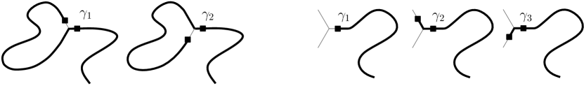
Figure 6. Left: a pair of walks visiting the three mid-edges and matched together. Right: a triplet of walks, one visiting one mid-edge, the two others visiting two mid-edges, which are matched together.

Let $\omega_{1}$ and $\omega_{2}$ be two walks that are grouped as in the first case. Without loss of generality, we assume that $\omega_{1}$ ends at $q$ and $\omega_{2}$ ends at $r$. Note that $\omega_{1}$ and $\omega_{2}$ coincide up to the mid-edge $p$ since $(\omega_{1},\omega_{2})$ are matched together. Then

(3.7) $$\ell(\omega_{1})=\ell(\omega_{2})\quad\quad\text{and}\quad\quad\left\{\ \begin{subarray}{c}{\rm W}_{\omega_{1}}(a,q)={\rm W}_{\omega_{1}}(a,p)+{\rm W}_{\omega_{1}}(p,q)={\rm W}_{\omega_{1}}(a,p)-\frac{4\pi}{3}\\ \ \\ {\rm W}_{\omega_{2}}(a,r)={\rm W}_{\omega_{2}}(a,p)+{\rm W}_{\omega_{2}}(p,r)={\rm W}_{\omega_{1}}(a,p)+\frac{4\pi}{3}.\end{subarray}\right.$$

In evaluating the winding of $\omega_{1}$ between $p$ and $q$, we used the fact that $a\in\partial\Omega$ and $\Omega$ is simply connected. The term $e^{-i\sigma{\rm W}_{\omega}(a,x)}$ gives a weight $\lambda$ or $\bar{\lambda}$ per left or right turn of $\omega$, where

(3.8) $$\lambda=\exp\left(-i\sigma\frac{\pi}{3}\right).$$

Writing $j=e^{i2\pi/3}$, we obtain

$$c(\omega_{1})+c(\omega_{2}) =(q-v)e^{-i\sigma{\rm W}_{\omega_{1}}(a,q)}z^{\ell(\omega_{1})}+(r-v)e^{-i\sigma{\rm W}_{\omega_{2}}(a,r)}z^{\ell(\omega_{2})}$$

(3.9) $$=(p-v)e^{-i\sigma{\rm W}_{\omega_{1}}(a,p)}z^{\ell(\omega_{1})}\left(j\bar{\lambda}^{4}+\bar{j}\lambda^{4}\right).$$

Now we set $\sigma=\frac{5}{8}$ so that $j\bar{\lambda}^{4}+\bar{j}\lambda^{4}=2\cos(\frac{3\pi}{2})=0$, and hence

(3.10) $$c(\omega_{1})+c(\omega_{2}) =0.$$

Let $\omega_{1},\omega_{2},\omega_{3}$ be three walks matched as in the second case. Without loss of generality, we assume that $\omega_{1}$ ends at $p$ and that $\omega_{2}$ and $\omega_{3}$ extend $\omega_{1}$ to $q$ and $r$ respectively. As before, we easily find that

(3.11) $$\ell(\omega_{2})=\ell(\omega_{3})=\ell(\omega_{1})+1\quad\quad\text{and}\quad\quad\left\{\ \begin{subarray}{c}{\rm W}_{\omega_{2}}(a,r)={\rm W}_{\omega_{2}}(a,p)+{\rm W}_{\omega_{2}}(p,q)={\rm W}_{\omega_{1}}(a,p)-\frac{\pi}{3}\\ \ \\ {\rm W}_{\omega_{3}}(a,r)={\rm W}_{\omega_{3}}(a,p)+{\rm W}_{\omega_{3}}(p,r)={\rm W}_{\omega_{1}}(a,p)+\frac{\pi}{3},\end{subarray}\right.$$

and thus

(3.12) $$c(\omega_{1})+c(\omega_{2})+c(\omega_{3}) =(p-v)e^{-i\sigma{\rm W}_{\omega_{1}}(a,p)}z^{\ell(\omega_{1})}\left(1+zj\bar{\lambda}+z\bar{j}\lambda\right).$$

Now we choose $z$ such that $1+zj\bar{\lambda}+z\bar{j}\lambda=0$. Due to our choice $\sigma=\frac{5}{8}$, we have $\lambda=\exp(-i\frac{5\pi}{24})$. Thus we choose $z_{c}^{-1}=2\cos\frac{\pi}{8}=\sqrt{2+\sqrt{2}}$.

Now the desired identity (3.5) follows immediately by summing over all the pairs and triplets of walks. ∎

The last step of the proof of Lemma 3.4 is the only place where the choice $z=z_{c}=1/\sqrt{2+\sqrt{2}}$ is used in the proof of Theorem 3.1.

3.2. Proof of Theorem 3.1 completed.

Now we will apply Lemma 3.4 to prove Theorem 3.1.

We consider a vertical strip domain $S_{T}$ composed of the vertices of $T$ strips of hexagons, and its finite version $S_{T,L}$ cut at height $L$ at an angle of $\frac{\pi}{3}$; see Figure 7. We denote the left and right boundaries of $S_{T}$ by $\alpha$ and $\beta$, respectively, and the top and bottom boundaries of $S_{T,L}$ by $\epsilon$ and $\bar{\epsilon}$, respectively. We also introduce the positive quantities:

(3.13) $$A_{T,L}(z) =\sum_{\begin{subarray}{c}\omega\subset S_{T,L}:\ a\rightarrow\alpha\setminus\{a\}\end{subarray}}z^{\ell(\omega)},$$

(3.14) $$B_{T,L}(z) =\sum_{\begin{subarray}{c}\omega\subset S_{T,L}:\ a\rightarrow\beta\end{subarray}}z^{\ell(\omega)},$$

(3.15) $$E_{T,L}(z) =\sum_{\begin{subarray}{c}\omega\subset S_{T,L}:\ a\rightarrow\epsilon\cup\bar{\epsilon}\end{subarray}}z^{\ell(\omega)}.$$

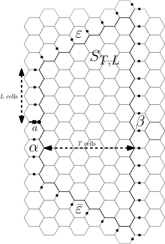
Figure 7. Domain $S_{T,L}$ and boundary parts $\alpha$, $\beta$, $\epsilon$ and $\bar{\epsilon}$.

Lemma 3.5.

For $z=z_{c}$,

(3.16) $$1=c_{\alpha}A_{T,L}(z_{c})+B_{T,L}(z_{c})+c_{\epsilon}E_{T,L}(z_{c}),$$

where $c_{\alpha}=\cos\left(\frac{3\pi}{8}\right)$ and $c_{\epsilon}=\cos\left(\frac{\pi}{4}\right)$.

Proof.

We fix $z=z_{c}$ and drop it from the notation. We sum the relation (3.5) over all vertices in $V(S_{T,L})$. Contributions at interior mid-edges vanish and we arrive at

(3.17) $$-\sum_{x\in\alpha}F(x)+\sum_{x\in\beta}F(x)+j\sum_{x\in\epsilon}F(x)+\bar{j}\sum_{x\in\bar{\epsilon}}F(x)=0.$$

The winding of any SAW from $a$ to the bottom part of $\alpha$ is $-\pi$, while the winding to the top part is $\pi$. Using this and symmetry, together with the fact that the only SAW from $a$ to $a$ has length $0$, we conclude that

(3.18) $$\sum_{x\in\alpha}F(x)=F(a)+\sum_{x\in\alpha\setminus\{a\}}F(x)=1+\frac{e^{-i\sigma\pi}+e^{i\sigma\pi}}{2}A_{T,L}=1-c_{\alpha}A_{T,L}.$$

Similarly, the winding from $a$ to any half-edge in $\beta$, $\epsilon$ or $\bar{\epsilon}$ is respectively $0$, $\frac{2\pi}{3}$ or $-\frac{2\pi}{3}$. Therefore, again using symmetry,

(3.19) $$\sum_{x\in\beta}F(x)=B_{T,L},\quad\quad j\sum_{x\in\epsilon}F(x)+\bar{j}\sum_{x\in\bar{\epsilon}}F(x)=c_{\epsilon}E_{T,L}.$$

The proof is completed by inserting (3.18)–(3.19) into (3.17). ∎

The sequences $(A_{T,L}(z))_{L>0}$ and $(B_{T,L}(z))_{L>0}$ are increasing in $L$ and are bounded for $z\leq z_{c}$, thanks to (3.16) and the monotonicity in $z$. Thus they have limits

(3.20) $$A_{T}(z) =\lim_{L\rightarrow\infty}A_{T,L}(z)=\sum_{\omega\subset S_{T}:\ a\rightarrow\alpha\setminus\{a\}}z^{\ell(\omega)},$$

(3.21) $$B_{T}(z) =\lim_{L\rightarrow\infty}B_{T,L}(z)=\sum_{\omega\subset S_{T}:\ a\rightarrow\beta}z^{\ell(\omega)}.$$

When $z=z_{c}$, via (3.16) again, we conclude that $(E_{T,L}(z_{c}))_{L>0}$ is decreasing and converges to a limit $E_{T}(z_{c})=\lim_{L\rightarrow\infty}E_{T,L}(z_{c})$. Thus, by (3.16),

(3.22) $$1=c_{\alpha}A_{T}(z_{c})+B_{T}(z_{c})+c_{\epsilon}E_{T}(z_{c}).$$

Proof of Theorem 3.1.

The bridge generating function is given by $B(z)=\sum_{T=0}^{\infty}B_{T}(z)$. Recall that it suffices to show that $B(z)<\infty$ for $z<z_{c}$, and that $B(z_{c})=\infty$ or $\chi(z_{c})=\infty$.

We first assume $z<z_{c}$. Since $B_{T}(z)$ involves only bridges of length at least $T$, it follows from (3.22) that

(3.23) $$B_{T}(z)\leq\left(\frac{z}{z_{c}}\right)^{T}B_{T}(z_{c})\leq\left(\frac{z}{z_{c}}\right)^{T},$$

and hence $B(z)$ is finite since the right-hand side is summable.

It remains to prove that $B(z_{c})=\infty$ or $\chi(z_{c})=\infty$. We do this by considering two separate cases. Suppose first that, for some $T$, $E_{T}(z_{c})>0$. As noted previously, $E_{T,L}(z_{c})$ is decreasing in $L$. Therefore, as required,

(3.24) $$\chi(z_{c})\geq\sum_{L=1}^{\infty}E_{T,L}(z_{c})\geq\sum_{L=1}^{\infty}E_{T}(z_{c})=\infty.$$

It remains to consider the case that $E^{z_{c}}_{T}=0$ for every $T$. In this case, (3.22) simplifies to

(3.25) $$1=c_{\alpha}A_{T}(z_{c})+B_{T}(z_{c}).$$

Observe that walks contributing to $A_{T+1}(z_{c})$ but not to $A_{T}(z_{c})$ must visit some vertex adjacent to the right edge of $S_{T+1}$. Cutting such a walk at the first such point (and adding half-edges to the two halves), we obtain two bridges of span $T+1$ in $S_{T+1}$. We conclude from this that

(3.26) $$A_{T+1}(z_{c})-A_{T}(z_{c})\leq z_{c}\left(B_{T+1}(z_{c})\right)^{2}.$$

Combining (3.25) for $T$ and $T+1$ with (3.26), we can write

$$0 =[c_{\alpha}A_{T+1}(z_{c})+B_{T+1}(z_{c})]-[c_{\alpha}A_{T}(z_{c})+B_{T}(z_{c})]$$

(3.27) $$\leq c_{\alpha}z_{c}\left(B_{T+1}(z_{c})\right)^{2}+B_{T+1}(z_{c})-B_{T}(z_{c}),$$

so

(3.28) $$c_{\alpha}z_{c}\left(B_{T+1}(z_{c})\right)^{2}+B_{T+1}(z_{c})\geq B_{T}(z_{c}).$$

It is an easy exercise to verify by induction that

(3.29) $$B_{T}(z_{c})\geq\min\{B_{1}(z_{c}),1/(c_{\alpha}z_{c})\}\frac{1}{T}$$

for every $T\geq 1$. This implies, as required, that

(3.30) $$B(z_{c})\geq\sum_{T=1}^{\infty}B_{T}(z_{c})=\infty.$$

This completes the proof. ∎

3.3. Conjecture 1.5 and the holomorphic observable

Recall the statement of Conjecture 1.5. When formulated on ${\mathbb{H}}$, this conjecture concerns a simply connected domain $\Omega$ in the complex plane $\mathbb{C}$ with two points $a$ and $b$ on the boundary, with a discrete approximation given by the largest finite domain $\Omega_{\delta}$ of $\delta{\mathbb{H}}$ included in $\Omega$, and with $a_{\delta}$ and $b_{\delta}$ the closest vertices of $\delta{\mathbb{H}}$ to $a$ and $b$ respectively. A probability measure $\mathbb{P}_{z,\delta}$ is defined on the set of SAWs $\omega$ between $a_{\delta}$ and $b_{\delta}$ that remain in $\Omega_{\delta}$ by assigning to $\omega$ a weight proportional to $z_{c}^{\ell(\omega)}$. We obtain a random curve denoted $\omega_{\delta}$. We can also define the observable in this context, and we denote it by $F_{\delta}$. Conjecture 1.5 then asserts that the random curve $\omega_{\delta}$ converges to $\mathrm{SLE}_{8/3}$ from $a$ and $b$ in the domain $\Omega$.

A possible approach to proving Conjecture 1.5 might be the following. First, prove a precompactness result for self-avoiding walks. Then, by taking a subsequence, we could assume that the curve $\gamma_{\delta}$ converges to a continuous curve (in fact, the limiting object would need to be a Loewner chain, see [1]). The second step would consist in identifying the possible limits. The holomorphic observable should play a crucial role in this step. Indeed, if $F_{\delta}$ converges when rescaled to an explicit function, one could use the martingale technique introduced in [70] to verify that the only possible limit is $\mathrm{SLE}_{8/3}$.

Regarding the convergence of $F_{\delta}$, we first recall that in the discrete setting contour integrals should be performed along dual edges. For ${\mathbb{H}}$, the dual edges form a triangular lattice, and Lemma 3.4 has the enlightening interpretation that the contour integral vanishes along any elementary dual triangle. Any area enclosed by a discrete closed dual contour is a union of elementary triangles, and hence the integral along any discrete closed contour also vanishes. This is a discrete analogue of Morera’s theorem. It implies that if the limit of $F_{\delta}$ (properly rescaled) exists and is continuous, then it is automatically holomorphic. By studying the boundary conditions, it is even possible to identify the limit. This leads to the following conjecture, which is based on ideas in [70].

Conjecture 3.6.

Let $\Omega$ be a simply connected domain (not equal to $\mathbb{C}$), let $z\in\Omega$, and let $a,b$ be two distinct points on the boundary of $\Omega$. We assume that the boundary of $\Omega$ is smooth near $b$. For $\delta>0$, let $F_{\delta}$ be the holomorphic observable in the domain $(\Omega_{\delta},a_{\delta},b_{\delta})$ approximating $(\Omega,a,b)$, and let $z_{\delta}$ be the closest point in $\Omega_{\delta}$ to $z$. Then

(3.31) $$\lim_{\delta\rightarrow 0}\frac{F_{\delta}(a_{\delta},z_{\delta})}{F_{\delta}(a_{\delta},b_{\delta})}=\left(\frac{\Phi^{\prime}(z)}{\Phi^{\prime}(b)}\right)^{5/8},$$

where $\Phi$ is a conformal map from $\Omega$ to the upper half-plane mapping a to $\infty$ and $b$ to 0.

The right-hand side of (3.31) is well-defined, since the conformal map $\Phi$ is unique up to multiplication by a real factor.

3.4. Loop models and holomorphic observables.

The original motivation for the introduction of the holomorphic observable stems from a more general context, which we now discuss. The loop $O(n)$ model is a lattice model on a domain $\Omega$. We restrict attention in this discussion to the hexagonal lattice ${\mathbb{H}}$. A configuration $\omega$ is a family of self-avoiding loops, and its probability is proportional to $z^{\#\text{edges}}n^{\#\text{loops}}$. The loop parameter $n$ is taken in $[0,2]$. There are other variants of the model; for instance, one can introduce an interface going from one point $a$ on the boundary to the inside, or one interface between two points of the boundary. The case $n=1$ corresponds to the Ising model, while the case $n=0$ corresponds to the self-avoiding walk (when allowing one interface).

Fix $n\in[0,2]$. It is a non-rigorous prediction of [61] that the model has the following three phases distinguished by the value of $z$:

• If $z<1/\sqrt{2+\sqrt{2-n}}$, the loops are sparse (typically of logarithmic size in the size of the domain). This phase is subcritical.

• If $z=1/\sqrt{2+\sqrt{2-n}}$, the loops are dilute (there are loops of the size of the domain which are typically separated be a distance of the size of the domain). This phase is critical.

• If $z>1/\sqrt{2+\sqrt{2-n}}$, the loops are dense (there are loops of the size of the domain which are typically separated be a distance much smaller than the size of the domain). This phase is critical as well.

Consider the special case of the Ising model at its critical value $z_{c}=1/\sqrt{3}$. Let $E$ denote the set of configurations consisting only of self-avoiding loops, and let $E(a,x)$ denote the set of configurations with self-avoiding loops plus an interface $\gamma$ from $a$ to $x$. Then, ignoring the issue of boundary conditions, the Ising spin-spin correlation is given in terms of the loop model by

(3.32) $$\left\langle\sigma(a)\sigma(x)\right\rangle=\frac{\sum_{\omega\in E(a,x)}z_{c}^{\#\text{edges}}}{\sum_{\omega\in E}z_{c}^{\#\text{edges}}}.$$

A natural operation in physics consists in flipping the sign of the coupling constant of the Ising model along a path from $a$ to $x$, in such a way that a monodromy is introduced: if we follow a path turning around $x$, spins are reversed after one whole turn. See, e.g., [65]. In terms of the loop representation, the spin-spin correlation $\left\langle\sigma(a)\sigma(x)\right\rangle_{\text{monodromy}}$ in this new Ising model is

(3.33) $$\left\langle\sigma(a)\sigma(x)\right\rangle_{\text{monodromy}}=\frac{\sum_{\omega\in E(a,x)}(-1)^{\#\text{turns of }\gamma\text{ around }x}z_{c}^{\#\text{edges}}}{\sum_{\omega\in E}z_{c}^{\#\text{edges}}}$$

where $\gamma$ is the interface between $a$ and $x$.

The numerator of the right-hand side of (3.33) can be rewritten as

(3.34) $$\sum_{\omega\in E(a,x)}e^{-i\frac{1}{2}{\rm W}_{\gamma}(a,x)}z^{\#\text{edges}}n^{\#\text{loops}}$$

with $n=1$. This is of the same form as the holomorphic observable (3.4). With general values of $n$, and with the freedom to choose the value of $\sigma\in[0,1]$, we obtain the observable

(3.35) $$F_{z}(x)=\sum_{\omega\in E(a,x)}e^{-i\sigma{\rm W}_{\gamma}(a,x)}z^{\#\text{edges}}n^{\#\text{loops}}.$$

The values of $\sigma$ and $z$ need to be chosen according to the value of $n$. If $\sigma=\sigma(n)$ satisfies $2\cos[(1+2\sigma)2\pi/3]=-n$ and $z=z(n)=1/\sqrt{2+\sqrt{2-n}}$, then the proof of Lemma 3.4 can be modified to yield its conclusion in this more general context.

To conclude this discussion, consider the loop $O(n)$ model with a family of self-avoiding loops and a single interface between two boundary points $a$ and $b$. For $n=1$ and $z=1/\sqrt{3}$, it has been proved that the interface converges to $\mathrm{SLE}_{3}$ [18]. For other values of $z$ and $n$, the following behaviour is conjectured [70].

Conjecture 3.7.

Fix $n\in[0,2]$. For $z=1/\sqrt{2+\sqrt{2-n}}$, the interface between $a$ and $b$ converges, as the lattice spacing goes to zero, to

(3.36) $$\mathrm{SLE}_{\kappa}\quad\text{with}\quad\kappa=\frac{4\pi}{2\pi-\arccos(-n/2)}.$$

For $z>1/\sqrt{2+\sqrt{2-n}}$, the interface between $a$ and $b$ converges, as the lattice spacing goes to zero, to

(3.37) $$\mathrm{SLE}_{\kappa}\quad\text{with}\quad\kappa=\frac{4\pi}{\arccos(-n/2)}.$$

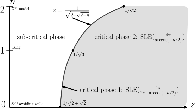
Figure 8. Phase diagram for $O(n)$ models.

Conjecture 3.7 is summarised in Figure 8. The value of $\arccos$ is in $[0,\pi]$, so the first regime corresponds to $\kappa\in[\frac{8}{3},4]$ and the second to $\kappa\in[4,8]$. These two critical regimes do not belong to the same universality class, in the sense that the scaling limit of the interface is not the same. In particular, since $\mathrm{SLE}_{\kappa}$ curves are simple for $\kappa\leq 4$ but not for $\kappa>4$ (see [1]), in the dilute phase the interface is conjectured to be simple in the scaling limit, but not in the dense phase. In addition, all the $\mathrm{SLE}_{\kappa}$ models for $\frac{8}{3}\leq\kappa\leq 8$ arise in these $O(n)$ models. This rich behaviour is at the heart of the mathematical interest in $O(n)$ models. To prove the conjecture remains a major challenge in 2-dimensional statistical mechanics.

4. The lace expansion

4.1. Main results

In dimensions $d\geq 5$, it has been proved that SAW has the same scaling behaviour as SRW. The following two theorems, due to Hara and Slade [33, 34] and to Hara [30], respectively, show that the critical exponents $\gamma,\nu,\eta$ exist and take the values $\gamma=1$, $\nu=\frac{1}{2}$, $\eta=0$, and that the scaling limit is Brownian motion.

Theorem 4.1.

Fix $d\geq 5$, and consider the nearest-neighbour SAW on $\mathbb{Z}^{d}$. There exist constants $A,D,\epsilon>0$ such that, as $n\to\infty$,

(4.1) $$c_{n} =A\mu^{n}[1+O(n^{-\epsilon})],$$

(4.2) $$\mathbb{E}_{n}\left\lvert\omega(n)\right\rvert^{2} =Dn[1+O(n^{-\epsilon})].$$

Also,

(4.3) $$\left(\frac{\omega(\left\lfloor nt\right\rfloor)}{\sqrt{Dn}}\right)_{t\geq 0} \to(B_{t})_{t\geq 0},$$

where $B_{t}$ denotes Brownian motion and the convergence is in distribution.

Theorem 4.2.

Fix $d\geq 5$, and consider the nearest-neighbour SAW on $\mathbb{Z}^{d}$. There are constants $c,\epsilon>0$ such that, as $x\to\infty$,

(4.4) $$G_{z_{c}}(x)=\frac{c}{\left\lvert x\right\rvert^{d-2}}\left[1+O\left(\left\lvert x\right\rvert^{-\epsilon}\right)\right].$$

The proofs are based on the lace expansion, a technique that was introduced by Brydges and Spencer [14] to study the weakly SAW in dimensions $d>4$. Since 1985, the method of lace expansion has been highly developed and extended to several other models: percolation ($d>6$), oriented percolation ($d>4$ spatial dimensions), the contact process ($d>4$), lattice trees and lattice animals ($d>8$), the Ising model ($d>4$), and to random subgraphs of high-dimensional transitive graphs such as the Boolean cube. For a review and references, see [69].

Versions of Theorems 4.1–4.2 have been proved also for spread-out models; see [57, 31]. More recently, the above two theorems have been extended also to study long-range SAWs based on simple random walks which take steps of length $r$ with probability proportional to $r^{-d-\alpha}$ for some $\alpha$. For $\alpha\in(0,2)$, the upper critical dimension (recall Section 1.6.4) is reduced from $4$ to $2\alpha$, and the Brownian limit is replaced by a stable law in dimensions $d>2\alpha$ [38]. Further results in this direction can be found in [39, 19].

Our goal now is modest. In this section, we will derive the lace expansion. In Section 5, we will sketch a proof of how it can be used to prove that $\gamma=1$, in the sense that

(4.5) $$\chi(z)\asymp\left(1-z/z_{c}\right)^{-1}\qquad\text{as $z\nearrow z_{c}$,}$$

both for the nearest-neighbour model with $d\geq d_{0}\gg 4$, and for the spread-out model with $L\geq L_{0}(d)\gg 1$ and any $d>4$. Here, the notation $f(z)\asymp g(z)$ means that there exist positive $c_{1},c_{2}$ such that $c_{1}g(z)\leq f(z)\leq c_{2}g(z)$ holds uniformly in $z$. The lower bound in (4.5) holds in all dimensions and follows immediately from the elementary observation in (1.12) that $c_{n}\geq\mu^{n}=z_{c}^{-n}$, since

(4.6) $$\chi(z)=\sum_{n=0}^{\infty}c_{n}z^{n}\geq\sum_{n=0}^{\infty}(\mu z)^{n}=\frac{1}{1-z/z_{c}}$$

for $z<z_{c}$. It therefore suffices to prove that in high dimensions we have the complementary upper bound

(4.7) $$\chi(z)\leq\frac{C}{1-z/z_{c}}$$

for some finite constant $C$.

4.2. The differential inequality for $\chi(z)$

We prove (4.7) by means of a differential inequality—an inequality relating $\tfrac{d}{dz}\chi(z)$ to $\chi(z)$. The derivation of the differential inequality and its implication for (4.7) first appeared in [3].

The differential inequality is expressed in terms of the quantity

(4.8) $${\sf B}(z)=\sum_{x\in\mathbb{Z}^{d}}G_{z}(x)^{2}$$

for $z\leq z_{c}$. Proposition 1.3 ensures that ${\sf B}(z)$ is finite for $z<z_{c}$. If we assume, as usual, that $G_{z_{c}}\sim c|x|^{-(d-2+\eta)}$, then ${\sf B}(z_{c})$ will be finite precisely when $d>4-2\eta$. With Fisher’s relation (1.40) and the predicted values of $\gamma$ and $\nu$ from (1.22) and (1.28), this inequality can be expected to hold, and correspondingly ${\sf B}(z_{c})<\infty$, only for $d>4$ (this is a prediction, not a theorem). We refer to ${\sf B}(z)$ as the bubble diagram because we express (4.8) diagramatically as

(4.9) $${\sf B}(z)=\raisebox{-18.7898pt}{\begin{picture}(0.0,0.0)\includegraphics{Bubble_pspdftex}\end{picture}\begin{picture}(1252.0,589.0)(1175.0,-716.0)\put(1201.0,-661.0){\makebox(0.0,0.0)[b]{\smash{{{\color[rgb]{0,0,0}$0$}}}}} \end{picture}}\,.$$

In this diagram, each line represents a factor $G_{z}(x)$ and the unlabelled vertex is summed over $x\in\mathbb{Z}^{d}$. The condition that ${\sf B}(z_{c})<\infty$ will be referred to as the bubble condition.

We now derive the differential inequality

(4.10) $$\frac{d}{dz}\left(z\chi(z)\right)\geq\frac{\chi(z)^{2}}{{\sf B}(z)}.$$

Assuming (4.10), we obtain (4.7) as if we were solving a differential equation. Namely, using the monotonicity of ${\sf B}$, we first replace ${\sf B}(z)$ by ${\sf B}(z_{c})$ in (4.10). We then rearrange and integrate from $z$ to $z_{c}$, using the terminal value $\chi(z_{c})=\infty$ from (4.6), to obtain

$$\frac{1}{z^{2}\chi(z)^{2}}\frac{d}{dz}\left(z\chi(z)\right) \geq\frac{1}{z^{2}{\sf B}(z_{c})}$$

$$-\frac{d}{dz}\left(\frac{1}{z\chi(z)}\right) \geq\frac{d}{dz}\left(\frac{-1}{z{\sf B}(z_{c})}\right)$$

$$-0+\frac{1}{z\chi(z)} \geq\frac{1}{{\sf B}(z_{c})}\left(-\frac{1}{z_{c}}+\frac{1}{z}\right)$$

(4.11) $$\frac{{\sf B}(z_{c})}{1-z/z_{c}} \geq\chi(z).$$

Thus we have reduced the proof of (4.5) to verifying (4.10) and showing that ${\sf B}(z_{c})<\infty$ in high dimensions. We will prove (4.10) now, and in Section 5 we will sketch the proof of the bubble condition in high dimensions.

We will use diagrams to derive (4.10). A proof using more conventional mathematical notation can be found, e.g., in [69]. In the diagrams in the next two paragraphs, each dot denotes a point in $\mathbb{Z}^{d}$, and if a dot is unlabelled then it is summed over all points in $\mathbb{Z}^{d}$. Each arc (or line) in a diagram represents a generating function for a SAW connecting the endpoints. At times SAWs corresponding to distinct lines must be mutually-avoiding. We will indicate this condition by labelling diagram lines and listing in groups those that mutually avoid.

With these conventions, we can describe the two-point function and the susceptibility succinctly by

(4.12) $$G_{z}(x)=\raisebox{-14.45377pt}{\begin{picture}(0.0,0.0)\includegraphics{Gzofx_pspdftex}\end{picture}\begin{picture}(1252.0,305.0)(1175.0,-641.0)\put(1201.0,-586.0){\makebox(0.0,0.0)[b]{\smash{{{\color[rgb]{0,0,0}$0$}}}}} \put(2401.0,-586.0){\makebox(0.0,0.0)[b]{\smash{{{\color[rgb]{0,0,0}$x$}}}}} \end{picture}}\,, \chi(z)=\raisebox{-14.45377pt}{\begin{picture}(0.0,0.0)\includegraphics{chiofz_pspdftex}\end{picture}\begin{picture}(1252.0,305.0)(1175.0,-641.0)\put(1201.0,-586.0){\makebox(0.0,0.0)[b]{\smash{{{\color[rgb]{0,0,0}$0$}}}}} \end{picture}}\,.$$

In order to obtain (4.10), let us consider $Q(z)=\frac{d}{dz}(z\chi(z))$. Note that $Q(z)$ can be regarded as the generating function for SAWs weighted by the number of vertices visited in the walk. We represent this diagrammatically as:

(4.13) $$Q(z)=\sum_{n=0}^{\infty}(n+1)c_{n}z^{n}=\raisebox{-23.84923pt}{\begin{picture}(0.0,0.0)\includegraphics{Qofz_pspdftex}\end{picture}\begin{picture}(2452.0,633.0)(1175.0,-796.0)\put(2401.0,-736.0){\makebox(0.0,0.0)[b]{\smash{{{\color[rgb]{0,0,0}$[12]$}}}}} \put(1201.0,-586.0){\makebox(0.0,0.0)[b]{\smash{{{\color[rgb]{0,0,0}$0$}}}}} \put(1801.0,-286.0){\makebox(0.0,0.0)[b]{\smash{{{\color[rgb]{0,0,0}$1$}}}}} \put(3001.0,-286.0){\makebox(0.0,0.0)[b]{\smash{{{\color[rgb]{0,0,0}$2$}}}}} \end{picture}}.$$

In (4.13), each segment represents a SAW path, and the notation [12] indicates that SAWs 1 and 2 must be mutually avoiding, apart from one shared vertex.

We apply inclusion-exclusion to (4.13), first summing over all pairs of SAWs, mutually avoiding or not, and then subtracting configurations where SAWs 1 and 2 intersect. We parametrise the subtracted term according to the last intersection point along the second walk. Renumbering the subwalks, we have

(4.14) $$Q(z)=\raisebox{-14.45377pt}{\begin{picture}(0.0,0.0)\includegraphics{QInc_pspdftex}\end{picture}\begin{picture}(1852.0,305.0)(1175.0,-641.0)\put(1201.0,-586.0){\makebox(0.0,0.0)[b]{\smash{{{\color[rgb]{0,0,0}$0$}}}}} \end{picture}}\>-\>\raisebox{-28.18524pt}{\begin{picture}(0.0,0.0)\includegraphics{QExcl_pspdftex}\end{picture}\begin{picture}(2452.0,1083.0)(1175.0,-871.0)\put(2026.0,-811.0){\makebox(0.0,0.0)[b]{\smash{{{\color[rgb]{0,0,0}$3$}}}}} \put(1201.0,-586.0){\makebox(0.0,0.0)[b]{\smash{{{\color[rgb]{0,0,0}$0$}}}}} \put(1426.0,-286.0){\makebox(0.0,0.0)[b]{\smash{{{\color[rgb]{0,0,0}$1$}}}}} \put(2626.0,89.0){\makebox(0.0,0.0)[b]{\smash{{{\color[rgb]{0,0,0}$4$}}}}} \put(3001.0,-811.0){\makebox(0.0,0.0)[b]{\smash{{{\color[rgb]{0,0,0}$[124][34]$}}}}} \put(2026.0,-511.0){\makebox(0.0,0.0)[b]{\smash{{{\color[rgb]{0,0,0}$2$}}}}} \end{picture}}$$

where the notation $[124][34]$ means that walks 1, 2 and 4 must be mutually avoiding except at the endpoints, whereas walk 3 must avoid walk 4 but is allowed to intersect walks 1 and 2. Also, SAWs 2 and 3 must each take at least one step. We obtain an inequality by relaxing the avoidance pattern to [14], keeping the requirement that the walk 23 should be non-empty:

$$Q(z) \geq\raisebox{-14.45377pt}{\begin{picture}(0.0,0.0)\includegraphics{QInc_pspdftex}\end{picture}\begin{picture}(1852.0,305.0)(1175.0,-641.0)\put(1201.0,-586.0){\makebox(0.0,0.0)[b]{\smash{{{\color[rgb]{0,0,0}$0$}}}}} \end{picture}}-\raisebox{-28.18524pt}{\begin{picture}(0.0,0.0)\includegraphics{QExclRelax_pspdftex}\end{picture}\begin{picture}(2452.0,1083.0)(1175.0,-871.0)\put(3001.0,-811.0){\makebox(0.0,0.0)[b]{\smash{{{\color[rgb]{0,0,0}$[14]$}}}}} \put(1201.0,-586.0){\makebox(0.0,0.0)[b]{\smash{{{\color[rgb]{0,0,0}$0$}}}}} \put(1426.0,-286.0){\makebox(0.0,0.0)[b]{\smash{{{\color[rgb]{0,0,0}$1$}}}}} \put(2626.0,89.0){\makebox(0.0,0.0)[b]{\smash{{{\color[rgb]{0,0,0}$4$}}}}} \end{picture}}$$

(4.15) $$=\chi(z)^{2}-Q(z)({\sf B}(z)-1).$$

Rearranging gives the inequality (4.10).

4.3. The lace expansion by inclusion-exclusion

The proof of the bubble condition is based on the lace expansion. The original derivation of the lace expansion by Brydges and Spencer [14] made use of a certain graphical construction called a lace. Later, it was realised that repeated inclusion-exclusion leads to the same expansion [68]. We present the inclusion-exclusion approach now; the approach via laces is treated in the problems of Section 4.4. The underlying graph plays little role in the derivation, and the following discussion pertains to either nearest-neighbour or spread-out SAWs. Indeed, with minor modifications, the discussion also applies on general graphs [22].

We use the convolution $(f*g)(x)=\sum_{y\in\mathbb{Z}^{d}}f(y)g(x-y)$ of two functions $f,g$ on $\mathbb{Z}^{d}$. The lace expansion gives rise to a formula for $c_{n}(x)$, for $n\geq 1$, of the form

(4.16) $$\begin{split}c_{n}(x)&=(c_{1}*c_{n-1})(x)+\sum_{m=2}^{n}(\pi_{m}*c_{n-m})(x)\\ &=\sum_{y\in\mathbb{Z}^{d}}c_{1}(y)c_{n-1}(x-y)+\sum_{m=2}^{n}\sum_{y\in\mathbb{Z}^{d}}\pi_{m}(y)c_{n-m}(x-y),\end{split}$$

in which the coefficients $\pi_{m}(y)$ are certain combinatorial integers that we will define below. Note that the identity (4.16) would hold for SRW with $\pi\equiv 0$. The quantity $\pi_{m}(y)$ can therefore be understood as a correction factor determining to what degree SAWs fail to behave like SRWs. In this sense, the lace expansion studies the SAW as a perturbation of the SRW.

Our starting point is similar to that of the derivation of the differential inequality (4.10), but now we will work with identities rather than inequalities. Also, rather than working with generating functions, we will work instead with walks with a fixed number of steps and without factors $z$: diagrams now arise from walks of fixed length. We begin by dividing an $n$-step SAW ($n\geq 1$) into its first step and the remainder of the walk. Because of self-avoidance, these two parts must be mutually avoiding, and we perform inclusion-exclusion on this condition:

$\displaystyle=\raisebox{-23.84923pt}{\begin{picture}(0.0,0.0)\includegraphics{c1ConvcAvoid_pspdftex}\end{picture}\begin{picture}(1252.0,633.0)(1175.0,-796.0)\put(1801.0,-736.0){\makebox(0.0,0.0)[b]{\smash{{{\color[rgb]{0,0,0}$[12]$}}}}} \put(1201.0,-586.0){\makebox(0.0,0.0)[b]{\smash{{{\color[rgb]{0,0,0}$0$}}}}} \put(2401.0,-586.0){\makebox(0.0,0.0)[b]{\smash{{{\color[rgb]{0,0,0}$x$}}}}} \put(1351.0,-286.0){\makebox(0.0,0.0)[b]{\smash{{{\color[rgb]{0,0,0}$1$}}}}} \put(1951.0,-286.0){\makebox(0.0,0.0)[b]{\smash{{{\color[rgb]{0,0,0}$2$}}}}} \end{picture}}$

(4.17) $$=\raisebox{-14.45377pt}{\begin{picture}(0.0,0.0)\includegraphics{c1Convc_pspdftex}\end{picture}\begin{picture}(1252.0,343.0)(1175.0,-641.0)\put(2401.0,-586.0){\makebox(0.0,0.0)[b]{\smash{{{\color[rgb]{0,0,0}$x$}}}}} \put(1201.0,-586.0){\makebox(0.0,0.0)[b]{\smash{{{\color[rgb]{0,0,0}$0$}}}}} \end{picture}}\>-\>\raisebox{-23.84923pt}{\begin{picture}(0.0,0.0)\includegraphics{LoopConvcAvoid_pspdftex}\end{picture}\begin{picture}(1398.0,1044.0)(1029.0,-796.0)\put(1801.0,-286.0){\makebox(0.0,0.0)[b]{\smash{{{\color[rgb]{0,0,0}$2$}}}}} \put(1201.0,-586.0){\makebox(0.0,0.0)[b]{\smash{{{\color[rgb]{0,0,0}$0$}}}}} \put(2401.0,-586.0){\makebox(0.0,0.0)[b]{\smash{{{\color[rgb]{0,0,0}$x$}}}}} \put(1501.0,14.0){\makebox(0.0,0.0)[b]{\smash{{{\color[rgb]{0,0,0}$1$}}}}} \put(1801.0,-736.0){\makebox(0.0,0.0)[b]{\smash{{{\color[rgb]{0,0,0}$[12]$}}}}} \end{picture}}$$

where \begin{picture}(352.0,126.0)(1025.0,-724.0)\end{picture} indicates a single step. In more detail, the first term on the right-hand side represents $(c_{1}*c_{n-1})(x)$, and the subtracted term represents the number of $n$-step walks from $0$ to $x$ which are self-avoiding apart from a single required return to $0$. We again perform inclusion-exclusion, first on the avoidance $[12]$ in the second term of (4.17) (noting now the first time along walk 2 that walk 1 is hit):

(4.18)

and then on the avoidance $$[34]$$ in the second term of (4.18) (noting the first time along walk 4 that walk 3 is hit):

(4.19)

The process is continued recursively. Since the total number $n$ of steps is finite, the above process terminates after a finite number of applications of inclusion-exclusion, because each application uses at least one step. The result is

$\displaystyle=\raisebox{-14.45377pt}{\begin{picture}(0.0,0.0)\includegraphics{c1Convc_pspdftex}\end{picture}\begin{picture}(1252.0,343.0)(1175.0,-641.0)\put(2401.0,-586.0){\makebox(0.0,0.0)[b]{\smash{{{\color[rgb]{0,0,0}$x$}}}}} \put(1201.0,-586.0){\makebox(0.0,0.0)[b]{\smash{{{\color[rgb]{0,0,0}$0$}}}}} \end{picture}}\>-\>\raisebox{-14.45377pt}{\begin{picture}(0.0,0.0)\includegraphics{LoopConvc_pspdftex}\end{picture}\begin{picture}(1398.0,889.0)(1029.0,-641.0)\put(1201.0,-586.0){\makebox(0.0,0.0)[b]{\smash{{{\color[rgb]{0,0,0}$0$}}}}} \put(2401.0,-586.0){\makebox(0.0,0.0)[b]{\smash{{{\color[rgb]{0,0,0}$x$}}}}} \end{picture}}$

(4.20) $$\quad+\>\raisebox{-23.84923pt}{\begin{picture}(0.0,0.0)\includegraphics{ThetaConvc_pspdftex}\end{picture}\begin{picture}(1466.0,920.0)(1111.0,-796.0)\put(1876.0,-736.0){\makebox(0.0,0.0)[b]{\smash{{{\color[rgb]{0,0,0}$[123]$}}}}} \put(2551.0,-136.0){\makebox(0.0,0.0)[b]{\smash{{{\color[rgb]{0,0,0}$x$}}}}} \put(1651.0,-436.0){\makebox(0.0,0.0)[b]{\smash{{{\color[rgb]{0,0,0}$3$}}}}} \put(1351.0,-136.0){\makebox(0.0,0.0)[b]{\smash{{{\color[rgb]{0,0,0}$2$}}}}} \put(1126.0,-61.0){\makebox(0.0,0.0)[b]{\smash{{{\color[rgb]{0,0,0}$1$}}}}} \put(1201.0,-586.0){\makebox(0.0,0.0)[b]{\smash{{{\color[rgb]{0,0,0}$0$}}}}} \end{picture}}\>-\>\raisebox{-23.84923pt}{\begin{picture}(0.0,0.0)\includegraphics{ThirdLaceConvc_pspdftex}\end{picture}\begin{picture}(1616.0,921.0)(1111.0,-796.0)\put(1951.0,-736.0){\makebox(0.0,0.0)[b]{\smash{{{\color[rgb]{0,0,0}$[1234][345]$}}}}} \put(2701.0,-586.0){\makebox(0.0,0.0)[b]{\smash{{{\color[rgb]{0,0,0}$x$}}}}} \put(1351.0,-136.0){\makebox(0.0,0.0)[b]{\smash{{{\color[rgb]{0,0,0}$2$}}}}} \put(1126.0,-61.0){\makebox(0.0,0.0)[b]{\smash{{{\color[rgb]{0,0,0}$1$}}}}} \put(1201.0,-586.0){\makebox(0.0,0.0)[b]{\smash{{{\color[rgb]{0,0,0}$0$}}}}} \put(1651.0,-511.0){\makebox(0.0,0.0)[b]{\smash{{{\color[rgb]{0,0,0}$3$}}}}} \put(2176.0,-61.0){\makebox(0.0,0.0)[b]{\smash{{{\color[rgb]{0,0,0}$5$}}}}} \put(1951.0,-136.0){\makebox(0.0,0.0)[b]{\smash{{{\color[rgb]{0,0,0}$4$}}}}} \end{picture}}\>+\dots$$

The first term on the right-hand side is just $(c_{1}*c_{n-1})(x)$. In the remaining terms on the right-hand side, we regard the line ending at $x$ as having length $n-m$, so that $m$ steps are used by the other lines. We also regard the line ending at $x$ as starting at $y$. A crucial fact is that the line ending at $x$ has no dependence on the other lines, so it represents $c_{n-m}(x-y)$. Thus, if we define the coefficients $\pi_{m}(y)$ as

$$\pi_{m}(y) =-\>\raisebox{-14.45377pt}{\begin{picture}(0.0,0.0)\includegraphics{Loop_pspdftex}\end{picture}\begin{picture}(343.0,889.0)(1029.0,-641.0)\put(1201.0,-586.0){\makebox(0.0,0.0)[b]{\smash{{{\color[rgb]{0,0,0}$0$}}}}} \end{picture}}\delta_{0y}+\>\raisebox{-23.84923pt}{\begin{picture}(0.0,0.0)\includegraphics{Theta_pspdftex}\end{picture}\begin{picture}(705.0,907.0)(1111.0,-721.0)\put(1501.0,-661.0){\makebox(0.0,0.0)[b]{\smash{{{\color[rgb]{0,0,0}$[123]$}}}}} \put(1651.0,-436.0){\makebox(0.0,0.0)[b]{\smash{{{\color[rgb]{0,0,0}$3$}}}}} \put(1351.0,-136.0){\makebox(0.0,0.0)[b]{\smash{{{\color[rgb]{0,0,0}$2$}}}}} \put(1126.0,-61.0){\makebox(0.0,0.0)[b]{\smash{{{\color[rgb]{0,0,0}$1$}}}}} \put(1201.0,-586.0){\makebox(0.0,0.0)[b]{\smash{{{\color[rgb]{0,0,0}$0$}}}}} \put(1801.0,51.0){\makebox(0.0,0.0)[b]{\smash{{{\color[rgb]{0,0,0}$y$}}}}} \end{picture}}\>-\>\raisebox{-23.84923pt}{\begin{picture}(0.0,0.0)\includegraphics{ThirdLace_pspdftex}\end{picture}\begin{picture}(1080.0,921.0)(1111.0,-796.0)\put(2101.0,-586.0){\makebox(0.0,0.0)[b]{\smash{{{\color[rgb]{0,0,0}\raisebox{1.66702pt}{$y$}}}}}} \put(1351.0,-136.0){\makebox(0.0,0.0)[b]{\smash{{{\color[rgb]{0,0,0}$2$}}}}} \put(1126.0,-61.0){\makebox(0.0,0.0)[b]{\smash{{{\color[rgb]{0,0,0}$1$}}}}} \put(1201.0,-586.0){\makebox(0.0,0.0)[b]{\smash{{{\color[rgb]{0,0,0}$0$}}}}} \put(1651.0,-511.0){\makebox(0.0,0.0)[b]{\smash{{{\color[rgb]{0,0,0}$3$}}}}} \put(2176.0,-61.0){\makebox(0.0,0.0)[b]{\smash{{{\color[rgb]{0,0,0}$5$}}}}} \put(1951.0,-136.0){\makebox(0.0,0.0)[b]{\smash{{{\color[rgb]{0,0,0}$4$}}}}} \put(1651.0,-736.0){\makebox(0.0,0.0)[b]{\smash{{{\color[rgb]{0,0,0}$[1234][345]$}}}}} \end{picture}}\>+\dotsc$$

(4.21) $$=\sum_{N=1}^{\infty}(-1)^{N}\pi_{m}^{(N)}(y),$$

where $\delta_{xy}=1_{\left\{x=y\right\}}$ denotes the Kronecker delta, then (4.20) becomes (4.16), namely

(4.22) $$c_{n}(x) =\sum_{y\in\mathbb{Z}^{d}}c_{1}(y)c_{n-1}(x-y)+\sum_{m=2}^{n}\sum_{y\in\mathbb{Z}^{d}}\pi_{m}(y)c_{n-m}(x-y).$$

By definition, $\pi_{m}^{(1)}(y)$ counts the number of $m$-step self-avoiding returns if $y=0$, and is otherwise $0$. Also, $\pi_{m}^{(2)}(y)$ counts the number of $m$-step “$\theta$-diagrams” with vertices $0$ and $y$, i.e., the number of $m$-step walks which start at zero, end at $y$, and are self-avoiding apart from a required return to $0$ and a visit to $y$ before terminating at $y$. With more attention to the inclusion-exclusion procedure, it can be seen that in the three diagrams on the right-hand side of (4.21) all the individual subwalks must have length at least $1$ except for subwalk 3 of the third term which may have length $0$. As noted above, the inclusion-exclusion procedure terminates after a finite number of steps, so the terms in the series (4.21) are eventually all zero, but as $m$ increases more and more terms are non-zero. If the diagrams make you uncomfortable, formulas for $\pi_{m}(y)$ are given in Section 4.4. This completes the derivation of the lace expansion.

Our next task is to relate $\pi_{m}(y)$ to our goal of proving the bubble condition. Equation (4.16) contains two convolutions: a convolution in space given by the sum over $y$, and a convolution in time given by the sum over $m$. To eliminate these and facilitate analysis, we pass to generating functions and Fourier transforms. By definition of the two-point function,

(4.23) $$G_{z}(x) =\sum_{n=0}^{\infty}c_{n}(x)z^{n}=\delta_{0x}+\sum_{n=1}^{\infty}c_{n}(x)z^{n},$$

and we define

(4.24) $$\Pi_{z}(x) =\sum_{m=2}^{\infty}\pi_{m}(x)z^{m}.$$

From (4.16), we obtain

(4.25) $$\begin{split}G_{z}(x)&=\delta_{0x}+\sum_{y\in\mathbb{Z}^{d}}zc_{1}(y)G_{z}(x-y)+\sum_{y\in\mathbb{Z}^{d}}\Pi_{z}(y)G_{z}(x-y)\\ &=\delta_{0x}+z(c_{1}*G_{z})(x)+(\Pi_{z}*G_{z})(x).\end{split}$$

Given an absolutely summable function $f:\mathbb{Z}^{d}\to\mathbb{C}$, we write its Fourier transform as

(4.26) $$\hat{f}(k)=\sum_{x\in\mathbb{Z}^{d}}f(x)e^{ik\cdot x},$$

with $k=(k_{1},\ldots,k_{d})\in[-\pi,\pi]^{d}$. Then (4.25) gives

(4.27) $$\hat{G}_{z}(k)=1+z\hat{c}_{1}(k)\hat{G}_{z}(k)+\hat{\Pi}_{z}(k)\hat{G}_{z}(k).$$

We solve for $\hat{G}_{z}(k)$ to obtain

(4.28) $$\hat{G}_{z}(k)=\frac{1}{1-z\hat{c}_{1}(k)-\hat{\Pi}_{z}(k)}.$$

It is convenient to express $c_{1}(y)$ in terms of the probability distribution for the steps of the corresponding SRW model:

(4.29) $$D(y)=\frac{c_{1}(y)}{\left\lvert\Omega\right\rvert},\qquad\qquad\hat{c}_{1}(k)=\left\lvert\Omega\right\rvert\hat{D}(k),$$

where $\left\lvert\Omega\right\rvert$ denotes the cardinality of either option for the set $\Omega$ defined in (1.1). For the nearest-neighbour model, $\left\lvert\Omega\right\rvert=2d$ and

(4.30) $$\hat{D}(k)=\frac{1}{2d}\sum_{j=1}^{d}\bigl{(}e^{ik_{j}}+e^{-ik_{j}}\bigr{)}=\frac{1}{d}\sum_{j=1}^{d}\cos k_{j}.$$

To simplify the notation, we define $\hat{F}_{z}(k)$ by

(4.31) $$\hat{G}_{z}(k)=\frac{1}{1-z\left\lvert\Omega\right\rvert\hat{D}(k)-\hat{\Pi}_{z}(k)}=\frac{1}{\hat{F}_{z}(k)}.$$

Notice that $\hat{G}_{z}(0)=\sum_{x\in\mathbb{Z}^{d}}\sum_{n=0}^{\infty}c_{n}(x)z^{n}=\chi(z)$, so that $\hat{G}_{z}(0)$ will have a singularity at $z=z_{c}$. To emphasise this, we will write

$$\hat{F}_{z}(k) =\hat{F}_{z}(0)+\bigl{(}\hat{F}_{z}(k)-\hat{F}_{z}(0)\bigr{)}$$

(4.32) $$=\chi(z)^{-1}+z\left\lvert\Omega\right\rvert\bigl{(}1-\hat{D}(k)\bigr{)}+\bigl{(}\hat{\Pi}_{z}(0)-\hat{\Pi}_{z}(k)\bigr{)}.$$

Now we can make contact with our goal of proving the bubble condition. By Parseval’s relation,

(4.33) $${\sf B}(z)=\sum_{x\in\mathbb{Z}^{d}}G_{z}(x)^{2}=\int_{[-\pi,\pi]^{d}}|\hat{G}_{z}(k)|^{2}\frac{d^{d}k}{(2\pi)^{d}}$$

(this includes the case where one side of the equality, and hence both, are infinite). The issue of whether ${\sf B}(z_{c})<\infty$ or not boils down to the question of whether the singularity of the integrand is integrable or not, so we will need to understand the asymptotics of the terms in (4.32) as $k\to 0$ and $z\nearrow z_{c}$. In principle there could be other singularities when $z=z_{c}$, but for the nearest-neighbour and spread-out models $1-\hat{D}(k)>0$ for non-zero $k$, and one of the goals of the analysis will be to prove that the term $\hat{\Pi}_{z}(0)-\hat{\Pi}_{z}(k)$ cannot create a cancellation.

The term $1-\hat{D}(k)$ is explicit, and for the nearest-neighbour model has asymptotic behaviour

(4.34) $$1-\hat{D}(k)=\frac{1}{d}\sum_{j=1}^{d}(1-\cos k_{j})\sim\frac{\left\lvert k\right\rvert^{2}}{2d}$$

as $k\to 0$. We need to see that the term $\hat{\Pi}_{z}(0)-\hat{\Pi}_{z}(k)$ is relatively small in high dimensions. By symmetry, we can write this term as

(4.35) $$\hat{\Pi}_{z}(0)-\hat{\Pi}_{z}(k) =\sum_{x\in\mathbb{Z}^{d}}(1-e^{ik\cdot x})\Pi_{z}(x)=\sum_{x\in\mathbb{Z}^{d}}(1-\cos k\cdot x)\Pi_{z}(x).$$

Finally, we note that the equation $\chi(z_{c})=\infty$ can be rewritten as $0=\chi(z_{c})^{-1}=1-z_{c}\left\lvert\Omega\right\rvert-\hat{\Pi}_{z_{c}}(0)$, from which we see that the critical point $z_{c}$ is given implicitly by

(4.36) $$z_{c}=\frac{1}{\left\lvert\Omega\right\rvert}\bigl{(}1-\hat{\Pi}_{z_{c}}(0)\bigr{)}.$$

This equation has been the starting point for the study of $z_{c}$, in particular for the derivation of the $1/d$ expansion for the connective constant discussed in Section 1.4. Problem 5.1 below indicates how the first terms are obtained.

4.4. Tutorial

These problems develop the original derivation of the lace expansion by Brydges and Spencer [14]. All this material can also be found in [69].

We require a notion of graphs on integer intervals, and connectivity of these graphs. We emphasise in advance that the notion of connectivity is not the usual graph theoretic one, but that it is the right notion in this context.

Definition 4.3.

(i) Let $I=[a,b]$ be an interval of non-negative integers. An edge is a pair $st=\{s,t\}$ with $s,t\in\mathbb{Z}$ and $a\leq s<t\leq b$. A graph on $[a,b]$ is a set of edges. We denote the set of all graphs on $[a,b]$ by $\mathcal{B}[a,b]$.

(ii) A graph $\Gamma\in\mathcal{B}[a,b]$ is connected if $a,b$ are endpoints of edges, and if for any $c\in(a,b)$, there are $s,t\in[a,b]$ such that $c\in(s,t)$ and $st\in\Gamma$. Equivalently, $\Gamma$ is connected if $(a,b)=\cup_{st\in\Gamma}(s,t)$. The set of all connected graphs on $[a,b]$ is denoted by $\mathcal{G}[a,b]$.

Problem 4.1.

Give an example of a graph which is connected in the above sense, but not path-connected in the usual graph theoretic sense, and give an example which is path-connected, but not connected in the above sense.

Let $U_{st}(\omega)=-1_{\left\{\omega(s)\neq\omega(t)\right\}}$, and for $a<b$ define

(4.37) $$K[a,b](\omega)=\prod_{a\leq s<t\leq b}(1+U_{st}(\omega)),\quad K[a,a](\omega)=1,$$

so that

(4.38) $$c_{n}(x)=\sum_{\omega\in\mathcal{W}_{n}(0,x)}K[0,n](\omega).$$

Problem 4.2.

Show that

(4.39) $$K[a,b](\omega)=\sum_{\Gamma\in\mathcal{B}[a,b]}\prod_{st\in\Gamma}U_{st}(\omega).$$

Problem 4.3.

For $a<b$, let

(4.40) $$J[a,b](\omega)=\sum_{\Gamma\in\mathcal{G}[a,b]}\prod_{st\in\Gamma}U_{st}(\omega).$$

Show that

(4.41) $$K[a,b]=K[a+1,b]+\sum_{j=a+1}^{b}J[a,j]K[j,b].$$

Problem 4.4.

Define

(4.42) $$\pi_{m}(x)=\sum_{\omega\in\mathcal{W}_{m}(0,x)}J[0,m](\omega)$$

for $m\geq 1$. Use Problem 4.3 to show that, for $n\geq 1$,

(4.43) $$c_{n}(x)=(c_{1}*c_{n-1})(x)+\sum_{m=1}^{n}(\pi_{m}*c_{n-m})(x).$$

(Compared to (4.16), the sum here starts at $m=1$ instead of $m=2$. In fact, we will see that $\pi_{1}(x)=0$ for the self-avoiding walk, since walks cannot self-intersect in 1 step.)

Definition 4.4.

A lace is a minimally connected graph, that is, a connected graph for which the removal of any edge would result in a disconnected graph. The set of laces on $[a,b]$ is denoted $\mathcal{L}[a,b]$.

Problem 4.5.

Let $L=\{s_{1}t_{1},\dots,s_{N}t_{N}\}$, where $s_{l}<t_{l}$ and $s_{l}\leq s_{l+1}$ for all $l$ (and all the edges are different). Show that $L$ is a lace if and only if

(4.44) $$a=s_{1}<s_{2},\quad s_{N}<t_{N-1}<t_{N}=b,\quad s_{l+1}<t_{l}\leq s_{l+2}\quad(1\leq l\leq N-2),$$

or $L=\left\{ab\right\}$ if $N=1$. In particular, for $N>1$, $L$ divides $[a,b]$ into $2N-1$ subintervals,

(4.45) $$[s_{1},s_{2}],[s_{2},t_{1}],[t_{1},s_{3}][s_{3},t_{2}],\dots,[t_{N-2},s_{N}][s_{N},t_{N-1}],[t_{N-1},t_{N}].$$

Determine which of these intervals must have length at least $1$, and which can have length $0$.

Let $\Gamma\in\mathcal{G}[a,b]$ be a connected graph. We associate a unique lace ${\sf L}_{\Gamma}$ to $\Gamma$ as follows: Let

(4.46) $$\begin{split}t_{1}=\max\{t:at\in\Gamma\},&\quad s_{1}=a,\\ t_{i+1}=\max\{t:\exists s<t_{i}\text{ such that }st\in\Gamma\},&\quad s_{i+1}=\min\{s:st_{i+1}\in\Gamma\}.\end{split}$$

The procedure terminates when $t_{N}=b$ for some $N$, and we then define ${\sf L}_{\Gamma}=\{s_{1}t_{1},\dots,s_{N}t_{N}\}$. We define the set of edges compatible with a lace $L\in\mathcal{L}[a,b]$ to be

(4.47) $$\mathcal{C}(L)=\{st:{\sf L}_{L\cup\{st\}}=L,st\notin L\}.$$

Problem 4.6.

Show that ${\sf L}_{\Gamma}=L$ if and only if $L\subset\Gamma$ and $\Gamma\setminus L\subset\mathcal{C}(L)$.

Problem 4.7.

Show that

(4.48) $$J[a,b](\omega)=\sum_{L\in\mathcal{L}[a,b]}\prod_{st\in L}U_{st}(\omega)\sum_{\Gamma:L_{\Gamma}=L}\prod_{s^{\prime}t^{\prime}\in\Gamma\setminus L}U_{s^{\prime}t^{\prime}}(\omega).$$

Conclude from the previous exercise that

(4.49) $$\sum_{\Gamma:{\sf L}_{\Gamma}=L}\prod_{s^{\prime}t^{\prime}\in\Gamma\setminus L}U_{s^{\prime}t^{\prime}}(\omega)=\prod_{s^{\prime}t^{\prime}\in\mathcal{C}(L)}(1+U_{s^{\prime}t^{\prime}}(\omega)),$$

and thus

(4.50) $$J[a,b](\omega)=\sum_{L\in\mathcal{L}[a,b]}\prod_{st\in L}U_{st}(\omega)\prod_{s^{\prime}t^{\prime}\in\mathcal{C}(L)}(1+U_{s^{\prime}t^{\prime}}(\omega)).$$

Problem 4.8.

Let $\mathcal{L}^{(N)}[a,b]$ denote the set of laces on $[a,b]$ which consist of exactly $N$ edges. Define

(4.51) $$J^{(N)}[a,b](\omega)=\sum_{L\in\mathcal{L}^{(N)}[a,b]}\prod_{st\in L}U_{st}(\omega)\prod_{s^{\prime}t^{\prime}\in\mathcal{C}(L)}(1+U_{s^{\prime}t^{\prime}}(\omega))$$

and

(4.52) $$\pi_{m}^{(N)}(x)=(-1)^{N}\sum_{\omega\in\mathcal{W}_{m}(0,x)}J^{(N)}[0,m](\omega).$$

1. Prove that

   (4.53) $$\pi_{m}(x)=\sum_{N=1}^{\infty}(-1)^{N}\pi_{m}^{(N)}(x)$$

   with $\pi_{m}^{(N)}(x)\geq 0$.

2. Describe the walk configurations that correspond to non-zero terms in $\pi_{m}^{(N)}(x)$, for $N=1,2,3,4$. What parts of the walk must be mutually avoiding?

3. What is the interpretation of the possibly empty intervals in Problem 4.5?

5. Lace expansion analysis in dimensions $d>4$

In this section, we outline a proof that the bubble condition holds for the nearest-neighbour model in sufficiently high dimensions, and for the spread-out model in dimensions $d>4$ provided $L$ is large enough. As noted above, the bubble condition implies that $\gamma=1$ in the sense that the susceptibility diverges linearly at the critical point as in (4.5). Proving the bubble condition will require control of the generating function $\hat{\Pi}_{z}(k)$ at the critical value $z=z_{c}$. According to (4.21) (see also Problem 4.8), $\Pi_{z}$ is given by an infinite series

(5.1) $$\Pi_{z}(x)=\sum_{N=1}^{\infty}(-1)^{N}\Pi_{z}^{(N)}(x),\qquad\Pi_{z}^{(N)}(x)=\sum_{m=2}^{\infty}\pi_{m}^{(N)}(x)z^{m}.$$

The lace expansion is said to converge if $\Pi_{z}(x)$ is absolutely summable when $z=z_{c}$, in the strong sense that

(5.2) $$\sum_{x\in\mathbb{Z}^{d}}\sum_{N=1}^{\infty}\Pi_{z_{c}}^{(N)}(x)<\infty.$$

There are now several different approaches to proving convergence of the lace expansion. In particular, a powerful but technically demanding method involves the study of (4.16) by induction on $n$ [41]. Here we will follow the relatively simple approach of [69], which was inspired by a similar argument for percolation in [2]. Some details are omitted below; these can all be found in [69].

We will make use of the usual $\ell^{p}$ norms on functions on $\mathbb{Z}^{d}$, for $p=1,2,\infty$. In addition, when dealing with functions on the torus $[-\pi,\pi]^{d}$, we will use the usual $L^{p}$ norms with respect to the probability measure $(2\pi)^{-d}d^{d}k$ on the torus, for $p=1,2$. To simplify the notation, we will sometimes omit the measure, and write, e.g., ${\sf B}(z)=\int\hat{G}_{z}^{2}=\|\hat{G}_{z}\|_{2}^{2}$.

5.1. Diagrammatic estimates

We will obtain bounds on $\Pi_{z}(x)$ in terms of $G_{z}(x)$ and the closely related quantity $H_{z}(x)$ defined by

(5.3) $$H_{z}(x)=G_{z}(x)-\delta_{0x}=\sum_{n=1}^{\infty}c_{n}(x)z^{n}.$$

The trivial term $c_{0}(x)=\delta_{0x}$ in $G_{z}(x)$ gives rise to a contribution $1$ in the bubble diagram, and it will be important in the following that this contribution sometimes be omitted. It is for this reason that we use $H_{z}$ as well as $G_{z}$.

The following diagrammatic estimates bound $\Pi_{z}$ in terms of $H_{z}$ and $G_{z}$. Once this theorem has been proved, the details of the definition of $\Pi_{z}$ are no longer needed—the rest of the argument is analysis that uses the diagrammatic estimates.

Theorem 5.1.

For any $z\geq 0$,

(5.4) $$\sum_{x\in\mathbb{Z}^{d}}\Pi_{z}^{(1)}(x) \leq z\left\lvert\Omega\right\rvert\left\lVert H_{z}\right\rVert_{\infty},$$

(5.5) $$\sum_{x\in\mathbb{Z}^{d}}(1-\cos k\cdot x)\Pi_{z}^{(1)}(x) =0,$$

and for $N\geq 2$,

(5.6) $$\sum_{x\in\mathbb{Z}^{d}}\Pi_{z}^{(N)}(x) \leq\left\lVert H_{z}\right\rVert_{\infty}\left\lVert G_{z}*H_{z}\right\rVert_{\infty}^{N-1},$$

(5.7) $$\sum_{x\in\mathbb{Z}^{d}}(1-\cos k\cdot x)\Pi_{z}^{(N)}(x) \leq N^{2}\left\lVert(1-\cos k\cdot x)H_{z}\right\rVert_{\infty}\left\lVert G_{z}*H_{z}\right\rVert_{\infty}^{N-1}.$$

Proof.

We prove just the cases $N=1,2$ here; the complete proof can be found in [69, Theorem 4.1].

For $N=1$, since $\pi_{m}^{(1)}(x)$ is equal to $\delta_{0x}$ times the number $\sum_{y\in\Omega}c_{m-1}(y)$ of self-avoiding returns, we have

(5.8) $$\sum_{x\in\mathbb{Z}^{d}}\Pi_{z}^{(1)}(x)=\sum_{y\in\Omega}\sum_{m=2}^{\infty}c_{m-1}(y)z^{m}=\sum_{y\in\Omega}zH_{z}(y),$$

which implies (5.4). Also, (5.5) follows from

(5.9) $$\sum_{x\in\mathbb{Z}^{d}}(1-\cos k\cdot x)\Pi_{z}^{(1)}(x)=(1-\cos k\cdot 0)\Pi_{z}^{(1)}(0)=0.$$

For $N=2$, dropping the mutual avoidance constraint between the three lines in $\pi_{m}^{(2)}(x)$ in (4.21) gives

$$\sum_{x\in\mathbb{Z}^{d}}\Pi_{z}^{(2)}(x) \leq\sum_{x\in\mathbb{Z}^{d}}H_{z}(x)^{3}\leq\left\lVert H_{z}\right\rVert_{\infty}(H_{z}*H_{z})(0)$$

(5.10) $$\leq\left\lVert H_{z}\right\rVert_{\infty}\left\lVert H_{z}*H_{z}\right\rVert_{\infty}$$

and

(5.11) $$\sum_{x\in\mathbb{Z}^{d}}(1-\cos k\cdot x)\Pi_{z}^{(2)}(x) \leq\left\lVert(1-\cos k\cdot x)H_{z}\right\rVert_{\infty}\left\lVert H_{z}*H_{z}\right\rVert_{\infty}.$$

Since $0\leq H_{z}(x)\leq G_{z}(x)$, this is stronger than (5.6) and (5.7). ∎

5.2. The small parameter

Theorem 5.1 shows that the sum over $N$ in (5.1) can be dominated by the sum of a geometric series with ratio $\left\lVert G_{z}*H_{z}\right\rVert_{\infty}$. Ideally, we would like this ratio to be small. A Cauchy–Schwarz estimate gives

$$\left\lVert H_{z}*G_{z}\right\rVert_{\infty} \leq\left\lVert H_{z}\right\rVert_{\infty}+\left\lVert H_{z}*H_{z}\right\rVert_{\infty}\leq\left\lVert H_{z}\right\rVert_{\infty}+\left\lVert H_{z}\right\rVert_{2}^{2}$$

(5.12) $$\leq\left\lVert H_{z}\right\rVert_{\infty}+\left\lVert G_{z}\right\rVert_{2}^{2}=\left\lVert H_{z}\right\rVert_{\infty}+{\sf B}(z),$$

but this looks problematic because the upper bound involves the bubble diagram —the very quantity we are trying to prove is finite at the critical point! So we will need some insight to make good use of the diagrammatic estimates.

An important idea will be to use not just the finiteness, but also the smallness of $H_{z}$. Specifically, we might hope that $\left\lVert H_{z_{c}}\right\rVert_{2}^{2}=\left\lVert\smash[t]{\hat{H}_{z_{c}}}\right\rVert_{2}^{2}=\left\lVert\smash[t]{\hat{G}_{z_{c}}-1}\right\rVert_{2}^{2}$ should be small when the corresponding quantity for SRW is small.

Let $C_{z}(x)=\sum_{n=0}c_{n}^{(0)}(x)z^{n}$ be the analogue of $G_{z}(x)$ for the SRW model. Its critical value is $z_{0}=\left\lvert\Omega\right\rvert^{-1}$, and

(5.13) $$\hat{C}_{z}(k)=\frac{1}{1-z\left\lvert\Omega\right\rvert\hat{D}(k)},\qquad\qquad\hat{C}_{z_{0}}(k)=\frac{1}{1-\hat{D}(k)}.$$

The SRW analogue of $\left\lVert\smash[t]{\hat{G}_{z_{c}}-1}\right\rVert_{2}^{2}$ is

(5.14) $$\left\lVert\smash[t]{\hat{C}_{z_{0}}-1}\right\rVert_{2}^{2}=\int\left(\frac{1}{1-\hat{D}}-1\right)^{2}=\int\frac{\hat{D}^{2}}{\bigl{(}1-\hat{D}\bigr{)}^{2}}.$$

The following elementary proposition shows that the above integral is small for the models we are studying. The hypothesis $d>4$ is needed for convergence, due to the $(|k|^{-2})^{2}$ singularity at the origin.

Proposition 5.2.

Let $d>4$. Then

(5.15) $$\int\frac{\hat{D}^{2}}{\bigl{(}1-\hat{D}\bigr{)}^{2}}\leq\beta$$

where, for some constant $K$,

(5.16) $$\beta=\begin{cases}\dfrac{K}{d-4}&\text{for the nearest-neighbour model,}\\ \text{\raisebox{0.0pt}[17.50002pt]{}}\dfrac{K}{L^{d}}&\text{for the spread-out model.}\end{cases}$$

Proof.

This is a calculus problem. For the nearest-neighbour model, see [57, Lemma A.3], and for the spread-out model see [69, Proposition 5.3]. ∎

We will prove the following theorem.

Theorem 5.3.

There are constants $\beta_{0}$ and $C$, independent of $d$ and $L$, such that when (5.15) holds with $\beta\leq\beta_{0}$ we have ${\sf B}(z_{c})\leq 1+C\beta$.

Theorem 5.3 achieves our goal of proving the bubble condition for the nearest-neighbour model in sufficiently high dimensions, and for the spread-out model with $L$ sufficiently large in dimensions $d>4$. As noted previously, this gives the following corollary that $\gamma=1$ in high dimensions.

Corollary 5.4.

When (5.15) holds with $\beta\leq\beta_{0}$, then as $z\nearrow z_{c}$,

(5.17) $$\chi(z)\asymp\frac{1}{1-z/z_{c}}.$$

5.3. Proof of Theorem 5.3

We begin with the following elementary lemma, which will be a principal ingredient in the proof.

Lemma 5.5.

Let $a<b$ be real numbers and let $f$ be a continuous real-valued function on $[z_{1},z_{2})$ such that $f(z_{1})\leq a$. Suppose that, for each $z\in(z_{1},z_{2})$, we have the implication

(5.18) $$f(z)\leq b\qquad\implies\qquad f(z)\leq a.$$

Then $f(z)\leq a$ for all $z\in[z_{1},z_{2})$.

Proof.

The result is a straightforward application of the Intermediate Value Theorem. ∎

Figure 9. The definition of $p(z)$.

We will apply Lemma 5.5 to a carefully chosen function $f$, based on a coupling between $\hat{G}$ on the parameter range $[0,z_{c})$, and the SRW analogue $\hat{C}$ on the parameter range $[0,z_{0})$. To define the coupling, let $z\in[0,z_{c})$ and define $p(z)\in[0,z_{0})$ by

(5.19) $$\hat{G}_{z}(0)=\chi(z)=\hat{C}_{p(z)}(0)=\frac{1}{1-p(z)\left\lvert\Omega\right\rvert},$$

i.e.,

(5.20) $$p(z)\left\lvert\Omega\right\rvert=1-\chi(z)^{-1}=z\left\lvert\Omega\right\rvert+\hat{\Pi}_{z}(0).$$

See Figure 9. We expect (or hope!) that $\hat{G}_{z}(k)\approx\hat{C}_{p(z)}(k)$ for all $k$, not just for $k=0$, as well as an additional condition that expresses another form of similarity between $\hat{G}_{z}(k)$ and $\hat{C}_{p(z)}(k)$. For the latter, we define

(5.21) $$-\tfrac{1}{2}\Delta_{k}\hat{G}_{z}(l)=\hat{G}_{z}(l)-\tfrac{1}{2}\bigl{(}\hat{G}_{z}(l+k)+\hat{G}_{z}(l-k)\bigr{)};$$

this is the Fourier transform of $(1-\cos k\cdot x)G_{z}(x)$ with $l$ as the dual variable. We aim to apply Lemma 5.5 with $z_{1}=0$, $z_{2}=z_{c}$, $a=1+{\rm const}\cdot\beta$ (with a constant whose value is determined in (5.27) below), $b=4$ (in fact, any fixed $b>1$ will do here), and

(5.22) $$f(z)=\max\left\{f_{1}(z),f_{2}(z),f_{3}(z)\right\}$$

where

(5.23) $$f_{1}(z)=z\left\lvert\Omega\right\rvert,\qquad f_{2}(z)=\sup_{k\in[-\pi,\pi]^{d}}\frac{|\hat{G}_{z}(k)|}{|\hat{C}_{p(z)}(k)|},$$

and

(5.24) $$f_{3}(z)=\sup_{k,l\in[-\pi,\pi]^{d}}\frac{\frac{1}{2}|\Delta_{k}\hat{G}_{z}(l)|}{|U_{p(z)}(k,l)|},$$

with

$$U_{p(z)}(k,l) =16\hat{C}_{p(z)}(k)^{-1}\left(\hat{C}_{p(z)}(l-k)\hat{C}_{p(z)}(l)+\hat{C}_{p(z)}(l+k)\hat{C}_{p(z)}(l)\right.$$

(5.25) $$\hskip 79.66771pt\left.+\hat{C}_{p(z)}(l-k)\hat{C}_{p(z)}(l+k)\right).$$

The choice of $U_{p(z)}(k,l)$ is made for technical reasons not explained here, and should be regarded as a useful replacement for the more natural choice $\frac{1}{2}|\Delta_{k}\hat{C}_{p(z)}(l)|$.

The conclusion from Lemma 5.5 would be that $f(z)\leq a$ for all $z\in[0,z_{c})$. The inequality (5.15) can be used to show that $\|(1-\hat{D})^{-1}\|_{2}^{2}\leq 1+3\beta$ (see [69, (5.10)]), and hence we may assume that $\|(1-\hat{D})^{-1}\|_{2}^{2}\leq 2$. Using $f_{2}(z)\leq a$ we therefore conclude that

$$B(z_{c}) =\lim_{z\nearrow z_{c}}B(z)=\lim_{z\nearrow z_{c}}\left\lVert\smash[t]{\hat{G}_{z}}\right\rVert_{2}^{2}$$

$$\leq a^{2}\lim_{z\nearrow z_{c}}\|\hat{C}_{p(z)}\|_{2}^{2}=a^{2}\bigl{\|}\bigl{(}1-\hat{D}\bigr{)}^{-1}\bigr{\|}_{2}^{2}$$

(5.26) $$\leq 2a^{2}<\infty$$

which is our goal. Thus it suffices to verify the hypotheses on $f(z)$ in Lemma 5.5. This is the content of the following lemma.

Lemma 5.6.

The function $f(z)$ defined by (5.22)–(5.24) is continuous on $[0,z_{c})$, with $f(0)=1$, and for each $z\in(0,z_{c})$,

(5.27) $$f(z)\leq 4\qquad\implies\qquad f(z)\leq 1+O(\beta).$$

Proof.

It is relatively easy to verify the continuity of $f$, and we omit the details. To see that $f(0)=1\leq a$, we observe that $f_{1}(0)=0$, $p(0)=0$ and hence $f_{2}(0)=1/1=1$, and $f_{3}(0)=0$. The difficult step is to prove the implication (5.27), and the remainder of the proof concerns this step. We assume throughout that $f(z)\leq 4$.

We consider first $f_{1}(z)=z\left\lvert\Omega\right\rvert$. Our goal is to prove that $f_{1}(z)\leq 1+O(\beta)$, and for this we will only use the assumptions $f_{1}(z)\leq 4$ and $f_{2}(z)\leq 4$; we do not yet need $f_{3}$. Since $0<\chi(z)<\infty$, we have $\chi(z)^{-1}=1-z\left\lvert\Omega\right\rvert-\hat{\Pi}_{z}(0)>0$, i.e.,

(5.28) $$f_{1}(z)=z\left\lvert\Omega\right\rvert<1-\hat{\Pi}_{z}(0)\leq 1+|\hat{\Pi}_{z}(0)|.$$

The required bound for $f_{1}(z)$ will follow once we show that for all $z\in(0,z_{c})$ and for all $k\in[-\pi,\pi]^{d}$,

(5.29) $$|\hat{\Pi}_{z}(k)|\leq O(\beta).$$

To prove (5.29) we use Theorem 5.1 (more precisely, (5.4) and (5.6)), to obtain

$$|\hat{\Pi}_{z}(k)| \leq\sum_{N=1}^{\infty}\sum_{x\in\mathbb{Z}^{d}}\Pi_{z}^{(N)}(x)$$

(5.30) $$\leq\left\lVert H_{z}\right\rVert_{\infty}\left(f_{1}(z)+\sum_{N=2}^{\infty}\left\lVert G_{z}*H_{z}\right\rVert_{\infty}^{N-1}\right).$$

For the first term, we use $f_{1}(z)\leq 4$. For the second term, we need a bound on $\left\lVert G_{z}*H_{z}\right\rVert_{\infty}$ in order to bound the sum. By definition,

(5.31) $$\left\lVert G_{z}*H_{z}\right\rVert_{\infty}\leq\left\lVert H_{z}\right\rVert_{\infty}+\left\lVert H_{z}*H_{z}\right\rVert_{\infty}\leq\left\lVert H_{z}\right\rVert_{\infty}+\left\lVert H_{z}\right\rVert_{2}^{2}.$$

Now $H_{z}$ is the generating function for SAWs which take at least one step. By omitting the avoidance constraint between the first step and subsequent steps, we obtain

(5.32) $$H_{z}(x)\leq z\left\lvert\Omega\right\rvert(D*G_{z})(x)\leq 4(D*G_{z})(x).$$

Thus we can bound the second term in (5.31), using $f_{2}(z)\leq 4$ and Proposition 5.2, as

$$\left\lVert H_{z}\right\rVert_{2}^{2} \leq 4^{2}\left\lVert D*G_{z}\right\rVert_{2}^{2}=4^{2}\bigl{\|}\hat{D}\hat{G}_{z}\bigr{\|}_{2}^{2}$$

$$\leq 4^{4}\bigl{\|}\hat{D}\hat{C}_{p(z)}\bigr{\|}_{2}^{2}=4^{4}\left\lVert D*C_{p(z)}\right\rVert_{2}^{2}$$

$$\leq 4^{4}\left\lVert D*C_{z_{0}}\right\rVert_{2}^{2}=4^{4}\bigl{\|}\hat{D}\bigl{(}1-\hat{D}\bigr{)}^{-1}\bigr{\|}_{2}^{2}$$

(5.33) $$\leq 4^{4}\beta.$$

Similar estimates show $\left\lVert H_{z}\right\rVert_{\infty}\leq O(\beta)$. If we substitute these estimates into (5.30), we obtain

(5.34) $$|\hat{\Pi}_{z}(k)|\leq C\beta\left(4+\sum_{N=2}^{\infty}(C\beta)^{N-1}\right)$$

for some constant $C$, so that (5.29) will hold for $\beta$ sufficiently small. This completes the proof for $f_{1}(z)$.

We next sketch the proof that $f_{2}(z)\leq 1+O(\beta)$. Recalling the notation $\hat{F}_{z}(k)=\hat{G}_{z}(k)^{-1}$ introduced in (4.31), and using the formulas (5.19) and (5.20) for $p(z)$, we obtain

$$\frac{\hat{G}_{z}(k)}{\hat{C}_{p(z)}(k)}-1 =\frac{1-p(z)\left\lvert\Omega\right\rvert\hat{D}(k)}{\hat{F}_{z}(k)}-1$$

$$=\frac{1-\bigl{(}z\left\lvert\Omega\right\rvert+\hat{\Pi}_{z}(0)\bigr{)}\hat{D}(k)-\hat{F}_{z}(k)}{\hat{F}_{z}(k)}$$

$$=\frac{-\hat{\Pi}_{z}(0)\hat{D}(k)+\hat{\Pi}_{z}(k)}{\hat{F}_{z}(k)}$$

(5.35) $$=\frac{\hat{\Pi}_{z}(0)\bigl{(}1-\hat{D}(k)\bigr{)}-\bigl{(}\hat{\Pi}_{z}(0)-\hat{\Pi}_{z}(k)\bigr{)}}{\hat{F}_{z}(k)}.$$

The bound $f_{3}(z)\leq 4$ and (5.7) can be used to show that $|\hat{\Pi}_{z}(0)-\hat{\Pi}_{z}(k)|\leq\linebreak O(\beta)\bigl{(}1-\hat{D}(k)\bigr{)}$ (see [69] for details); it is precisely at this point that the need to include $f_{3}$ in the definition of $f$ arises. Together with (5.29), this shows that the numerator of (5.35) is $O(\beta)\bigl{(}1-\hat{D}(k)\bigr{)}$.

For the denominator, we recall the formula (4.32):

(5.36) $$\hat{F}_{z}(k)=\chi(z)^{-1}+z\left\lvert\Omega\right\rvert\bigl{(}1-\hat{D}(k)\bigr{)}+\bigl{(}\hat{\Pi}_{z}(0)-\hat{\Pi}_{z}(k)\bigr{)}.$$

To bound $\hat{F}_{z}(k)$ from below, we consider two parameter ranges for $z$. If $z\leq\tfrac{1}{2}\left\lvert\Omega\right\rvert^{-1}$, we can make the trivial estimate $\chi(z)^{-1}\geq\hat{C}_{z}(0)^{-1}=1-z\left\lvert\Omega\right\rvert\geq\tfrac{1}{2}$, so that $\hat{F}_{z}(k)\geq\tfrac{1}{2}+0-O(\beta)\geq\tfrac{1}{4}$ for small $\beta$. Since the numerator of (5.35) is itself $O(\beta)$, this proves that $f_{2}(z)\leq 1+O(\beta)$ for this range of $z$.

It remains to consider $\tfrac{1}{2}\left\lvert\Omega\right\rvert^{-1}\leq z\leq z_{c}$. Now we estimate

(5.37) $$\hat{F}_{z}(k)\geq 0+\tfrac{1}{2}\bigl{(}1-\hat{D}(k)\bigr{)}-O(\beta)\bigl{(}1-\hat{D}(k)\bigr{)}\geq\tfrac{1}{4}\bigl{(}1-\hat{D}(k)\bigr{)}.$$

The factors $1-\hat{D}(k)$ in the numerator and denominator of (5.35) cancel, leaving $O(\beta)$ as desired.

Finally the proof for $f_{3}(z)$ is similar to the proof for $f_{2}(z)$, and we refer to [69] for the details. ∎

5.4. Tutorial

For simplicity, we restrict our attention now to the nearest-neighbour model of SAWs in dimensions sufficiently high that the preceding arguments and conclusions apply. In Lemma 5.6, we found that $f_{2}(z)\leq a=1+O(d^{-1})$, since $\beta\leq O((d-4)^{-1})=O(d^{-1})$. This estimate, which states that

(5.38) $$\hat{G}_{z}(k)\leq a\hat{C}_{p(z)}(k)\qquad k\in[\-\pi,\pi]^{d},\;\;\;z\in(0,z_{c}),$$

is most important for $k\approx 0$, the small frequencies, and it is referred to as the infrared bound. Other bounds obtained in Lemma 5.6 can be framed as follows: there is a constant $c$, independent of $z\leq z_{c}$, such that

(5.39) $$\|H_{z}\|_{2}^{2}\leq cd^{-1},\quad\|H_{z}\|_{\infty}\leq cd^{-1},\quad\|\Pi_{z}\|_{1}\leq cd^{-1},$$

and

(5.40) $$\|\Pi_{z}^{(N)}\|_{1}\leq(cd^{-1})^{N},\quad\sum_{N=M}^{\infty}\|\Pi_{z}^{(N)}\|_{1}\leq cd^{-M}.$$

We also recall that the Fourier transform of the two-point function can be written as

(5.41) $$\hat{G}_{z}(k)=\frac{1}{1-z|\Omega|\hat{D}(k)-\hat{\Pi}_{z}(k)}.$$

Since $\hat{G}_{z}(0)\to\infty$ as $z\to z_{c}$, we obtain the equation

(5.42) $$1-z_{c}|\Omega|-\hat{\Pi}_{z_{c}}(0)=0.$$

This equation provides a starting point to study the connective constant $\mu=z_{c}^{-1}$.

Problem 5.1.

In this problem, we show that the connective constant obeys

(5.43) $$\mu=2d-1-(2d)^{-1}+O((2d)^{-2})\qquad\text{as $d\to\infty$.}$$

This special case of the results discussed in Section 1.4 was first proved by Kesten [51], by very different means.

(a) Let $m\geq 1$ be an integer. Show that $\|(1-\hat{D})^{-m}\|_{1}$ is non-increasing in $d>2m$. In particular, it follows that $\|\hat{C}_{z_{0}}\|_{2}$ is bounded uniformly in $d>4$.

Hint: $A^{-m}=\Gamma(m)^{-1}\int_{0}^{\infty}u^{m-1}e^{-uA}\;du$.

(b) Let $H^{(j)}_{z}(x)=\sum_{m=j}^{\infty}c_{m}(x)z^{m}$ be the generating function for SAWs that take at least $j$ steps. By relaxing the condition of mutual self-avoidance for the first $j$ steps, show that

(5.44) $$\|H^{(j)}_{z_{c}}\|_{\infty}\leq O((2d)^{-j/2}),\quad j>1.$$

Hint: Use the infrared bound for the two-point function (5.38), and that the probability that a $2j$-step simple random walk which starts at $0$ also ends at $0$ is

(5.45) $$\|\hat{D}^{2j}\|_{1}\leq O((2d)^{-j}).$$

(c) Recall that $\pi^{(1)}_{n}(x)=0$ if $x\neq 0$, so that $\hat{\Pi}^{(1)}_{z}(0)=\sum_{x\in\mathbb{Z}^{d}}\Pi^{(1)}_{z}(x)=\Pi^{(1)}_{z}(0)$ is the generating function for all self-avoiding returns. Prove that

(5.46) $$\hat{\Pi}^{(1)}_{z_{c}}(0)=(2d)^{-1}+3(2d)^{-2}+O((2d)^{-3})$$

(d) Note that $\hat{\Pi}^{(2)}_{z}(0)$ is the generating function for all $\theta$-walks: paths that visit their eventual endpoint, return to the origin, then return to their endpoint, and are otherwise self-avoiding. Prove that

(5.47) $$\hat{\Pi}^{(2)}_{z}(0)=(2d)^{-2}+O((2d)^{-3}).$$

(e) Conclude from (c) and (d) that

(5.48) $$\hat{\Pi}_{z}(0)=-(2d)^{-1}-2(2d)^{-2}+O((2d)^{-3}),$$

and use this to show

(5.49) $$\mu=2d-1-(2d)^{-1}+O((2d)^{-2}).$$

We have seen in Section 4.2 that $\chi(z)\asymp(1-z/z_{c})^{-1}$ in high dimensions, assuming the bubble condition. The next problem shows that this bound can be improved to an asymptotic formula.

Problem 5.2.

(a) Show that

(5.50) $$\frac{d[z\chi(z)]}{dz}=V(z)\chi(z)^{2},\quad\text{where }V(z)=1-\hat{\Pi}_{z}(0)+z\frac{d\hat{\Pi}_{z}(0)}{dz}.$$

Hint: Let $\hat{F}_{z}(0)=\chi(z)^{-1}=1-z|\Omega|-\hat{\Pi}_{z}(0)$ and express the left-hand side in terms of $\hat{F}_{z}(0)$.

(b) Show that $\hat{\Pi}_{z_{c}}(0)$, $\frac{d}{dz}\hat{\Pi}_{z_{c}}(0)$ and thus $V(z_{c})$ are finite. It follows that

(5.51) $$\frac{d[z\chi(z)]}{dz}=V(z)\chi(z)^{2}\sim V(z_{c})\chi(z)^{2}\quad\text{ as $z\nearrow z_{c}$,}$$

where $f(z)\sim g(z)$ means $\lim_{z\nearrow z_{c}}f(z)/g(z)=1$.

(c) Prove that $\chi(z)\sim A(1-z/z_{c})^{-1}$ as $z\nearrow z_{c}$, where the constant $A$ is given by $A=z_{c}^{-1}[2d+\frac{d}{dz}|_{z=z_{c}}\hat{\Pi}_{z}(0)]^{-1}$.

6. Integral representation for walk models

It has long been understood by physicists that it is sometimes possible to represent random fields by random walks. Ideas in this direction due to Symanzik [71] were influential among mathematicians, and inspired, e.g., the analysis of [6, 7] who showed how to use random walks to represent and analyse ferromagnetic lattice spin systems. In this section, we develop representations of two random walk models in terms of random fields, via functional integrals. Our ultimate goal is rather the opposite to that of [6, 7], namely we wish to study models of random walks via studying their integral representations. This will be the topic of Section 7.

We begin in Section 6.1 with some background material about Gaussian integrals. In Section 6.2, we use these Gaussian integrals to represent a model of SAWs in a background of self-avoiding loops, a model closely related to the $O(n)$ loop model discussed in Section 3.4. The random field in these Gaussian integrals is called a boson field in physics. It was realised in the physics literature [59, 63] that the loops in the loop model could be eliminated by the use of anti-commuting variables, referred to as a fermion field, thereby providing a representation for models of SAWs. The anti-commuting variables can be understood in terms of differential forms with their anti-commuting wedge product, and in Sections 6.3–6.4 we provide the relevant background on differential forms and their integration. Finally, in Section 6.5, we obtain an integral representation for SAWs. The ideas in this section are developed in further detail in [11].

6.1. Gaussian integrals

Fix a positive integer $M$. Later, we identify the set $\{1,\dots,M\}$ with a finite set $\Lambda$ on which the walks related to the fields take place, e.g., $\Lambda\subset\mathbb{Z}^{d}$. Consider a two-component real field

(6.1) $$(u,v)=(u_{x},v_{x})_{x\in\{1,\dots,M\}}\in\mathbb{R}^{M}\times\mathbb{R}^{M}.$$

From this, we obtain the associated complex field $(\varphi,\bar{\varphi})=(\varphi_{x},\bar{\varphi}_{x})_{x\in\{1,\dots,M\}}$, where

(6.2) $$\varphi_{x}=u_{x}+iv_{x},\quad\bar{\varphi}_{x}=u_{x}-iv_{x};$$

this is the so-called boson field. We wish to integrate with respect to the variables $(\varphi_{x},\bar{\varphi}_{x})$, and for this we will use the differentials $d\varphi_{x}=du_{x}+i\,dv_{x}$ and $d\bar{\varphi}_{x}=du_{x}-i\,dv_{x}$. As we will discuss in more detail in Section 6.3, differentials are multiplied using an anti-commuting product, so in particular $du_{x}\,dv_{x}=-dv_{x}\,du_{x}$, $du_{x}\,du_{x}=dv_{x}\,dv_{x}=0$, and $d\bar{\varphi}_{x}\,d\varphi_{x}=2i\,du_{x}\,dv_{x}$.

Let $C=(C_{xy})_{x,y\in\{1,\dots,M\}}$ be an $M\times M$ complex matrix with positive Hermitian part, meaning that

(6.3) $$\sum_{x,y=1}^{M}\varphi_{x}(C_{xy}+\bar{C}_{yx})\bar{\varphi}_{y}>0\quad\text{for all $\varphi\neq 0$ in $\mathbb{C}^{M}$.}$$

It is not difficult to see that this implies that $A=C^{-1}$ exists. The (complex) Gaussian measure with covariance $C$ is defined by

(6.4) $$d\mu_{C}(\varphi,\bar{\varphi})=\frac{1}{Z_{C}}e^{-\varphi A\bar{\varphi}}\;d\bar{\varphi}\,d\varphi,$$

where $\varphi A\bar{\varphi}=\sum_{x,y=1}^{M}\varphi_{x}A_{xy}\bar{\varphi}_{y}$, and

(6.5) $$d\bar{\varphi}\,d\varphi=d\bar{\varphi}_{1}\,d\varphi_{1}\cdots d\bar{\varphi}_{M}\,d\varphi_{M}=(2i)^{M}du_{1}\,dv_{1}\cdots du_{M}\,dv_{M}$$

is a multiple of the Lebesgue measure on $\mathbb{R}^{2M}$. The normalisation constant

(6.6) $$Z_{C}=\int_{\mathbb{R}^{2M}}e^{-\varphi A\bar{\varphi}}\;d\bar{\varphi}\,d\varphi$$

can be computed explicitly.

Lemma 6.1.

For $C$ with positive Hermitian part, the normalisation of the Gaussian integral is given by

(6.7) $$Z_{C}=\frac{(2\pi i)^{M}}{\det A}.$$

Proof.

In this proof, we make the simplifying assumption that $C$ and thus also $A$ are Hermitian, though the result holds more generally; see [11]. By the spectral theorem for Hermitian matrices, there is a positive diagonal matrix $D=\mathrm{diag}(d_{x})$ and a unitary matrix $U$ such that $A=U^{-1}DU$. Then, $\varphi A\bar{\varphi}=\rho D\bar{\rho}$ where $\rho=\bar{U}\varphi$ ($\bar{U}$ is the complex conjugate of $U$). By a change of variables in the integral and explicit computation of the resulting 1-dimensional integral,

(6.8) $$Z_{C}=\prod_{x=1}^{M}\int_{\mathbb{R}^{2}}e^{-d_{x}(u_{x}^{2}+v_{x}^{2})}\;2i\,du_{x}\,dv_{x}=\frac{(2\pi i)^{M}}{\prod_{x=1}^{M}d_{x}}=\frac{(2\pi i)^{M}}{\det A}.\qed$$

We define the differential operators

(6.9) $$\frac{\partial}{\partial\varphi_{x}}=\frac{1}{2}\left(\frac{\partial}{\partial u_{x}}-i\frac{\partial}{\partial v_{x}}\right),\quad\frac{\partial}{\partial\bar{\varphi}_{x}}=\frac{1}{2}\left(\frac{\partial}{\partial u_{x}}+i\frac{\partial}{\partial v_{x}}\right).$$

It is easy to check that

(6.10) $$\frac{\partial\varphi_{y}}{\partial\varphi_{x}}=\frac{\partial\bar{\varphi}_{y}}{\partial\bar{\varphi}_{x}}=\delta_{xy},\quad\frac{\partial\bar{\varphi}_{y}}{\partial\varphi_{x}}=\frac{\partial\varphi_{y}}{\partial\bar{\varphi}_{x}}=0.$$

The following integration by parts formula will be useful.

Lemma 6.2.

For $C$ with positive Hermitian part, and for nice functions $F$,

(6.11) $$\int\bar{\varphi}_{a}F\;d\mu_{C}(\varphi,\bar{\varphi})=\sum_{x=1}^{M}C_{ax}\int\frac{\partial F}{\partial\varphi_{x}}\;d\mu_{C}(\varphi,\bar{\varphi}).$$

Proof.

Integrating by parts, we obtain

$$\int\frac{\partial F}{\partial\varphi_{x}}e^{-\varphi A\bar{\varphi}}\;d\bar{\varphi}\,d\varphi =-\int F\frac{\partial}{\partial\varphi_{x}}e^{-\varphi A\bar{\varphi}}\;d\bar{\varphi}\,d\varphi$$

(6.12) $$=\int F\sum_{y}A_{xy}\bar{\varphi}_{y}e^{-\varphi A\bar{\varphi}}\;d\bar{\varphi}\,d\varphi.$$

It follows from the fact that $C=A^{-1}$ that

(6.13) $$\sum_{x=1}^{M}C_{ax}\int\frac{\partial F}{\partial\varphi_{x}}\;d\mu_{C}=\int\sum_{x,y}C_{ax}A_{xy}\bar{\varphi}_{y}F\;d\mu_{C}=\int\bar{\varphi}_{a}F\;d\mu_{C}.\qed$$

The following application of Lemma 6.2 is a special case of Wick’s Theorem. The quantity appearing on the right-hand side of (6.14) is the permanent of the submatrix of $C$ indexed by $(x_{i},y_{j})_{i,j=1}^{k}$.

Lemma 6.3.

Let $\{x_{1},\dots,x_{k}\}$ and $\{y_{1},\dots,y_{k}\}$ each be sets with $k$ distinct elements from $\{1,\dots,M\}$. Then

(6.14) $$\int\prod_{l=1}^{k}\bar{\varphi}_{x_{l}}\varphi_{y_{l}}d\mu_{C}=\sum_{\sigma\in S_{k}}\prod_{l=1}^{k}C_{x_{l},y_{\sigma(l)}},$$

where the sum is over the set $S_{k}$ of permutations of $\{1,\ldots,k\}$.

Proof.

This follows by repeated application of the integration by parts formula in Lemma 6.2. Each time the formula is applied, one factor of $\bar{\varphi}$ disappears on the right-hand side of (6.11), and the partial differentiation eliminates one factor $\varphi$ as well. ∎

6.2. Integral representation for a loop model

Let $\Lambda$ be a finite set of cardinality $M$. Fix $a,b\in\Lambda$ and a subset $X\subset\Lambda\setminus\{a,b\}$. An example we have in mind is $\Lambda\subset\mathbb{Z}^{d}$ and $X=\Lambda\setminus\{a,b\}$. We define the integral

(6.15) $$G_{ab,X}=\int\bar{\varphi}_{a}\varphi_{b}\prod_{x\in X}(1+\varphi_{x}\bar{\varphi}_{x})\;d\mu_{C}.$$

As we now explain, this can be interpreted as a loop model whose configurations consist of a self-avoiding walk from $a$ to $b$ whose intermediate steps lie in $X$, together with a background of closed loops in $X$. We denote by $\mathcal{S}_{ab}(X)$ the set of sequences $(a,x_{1},\ldots,x_{n-1},b)$ with $n\geq 1$ arbitrary and the $x_{i}\in X$ distinct—these are SAWs with rather general steps.

Repeated integration by parts gives

(6.16) $$G_{ab,X}=\sum_{\omega\in\mathcal{S}_{ab}(X)}C^{\omega}\int\prod_{x\in X\setminus\omega}(1+\varphi_{x}\bar{\varphi}_{x})\;d\mu_{C},$$

where $C^{\omega}=\prod_{i=1}^{\ell(\omega)}C_{w(i-1),w(i)}$. Also, by expanding the product and applying Lemma 6.3, we obtain

$$\int\prod_{x\in X\setminus\omega}(1+\varphi_{x}\bar{\varphi}_{x})\;d\mu_{C} =\sum_{Z\subset X\setminus\omega}\int\prod_{x\in Z}\varphi_{x}\bar{\varphi}_{x}\;d\mu_{C}$$

(6.17) $$=\sum_{Z\subset X\setminus\omega}\sum_{\sigma\in S(Z)}\prod_{z\in Z}C_{z,\sigma(z)},$$

with $S(Z)$ is the set of permutations of the set $Z$. Altogether, this gives

(6.18) $$G_{ab,X} =\sum_{\omega\in\mathcal{S}_{ab}(X)}C^{\omega}\sum_{Z\subset X\setminus\omega}\sum_{\sigma\in S(Z)}\prod_{z\in Z}C_{z,\sigma(z)}.$$

Thus, by decomposing the permutation $\sigma$ into cycles, we can interpret (6.15) as the generating function for self-avoiding walks from $a$ to $b$ in a background of loops with weight $C_{xy}$ for every step between $x$ and $y$ (with each loop corresponding to a cycle of $\sigma$). See Figure 10.

Figure 10. Self-avoiding walk from $a$ to $b$ with loop background. Loops can have length zero. The loops will be eliminated by the use of differential forms.

6.3. Differential forms

Our next goal is to modify the example of Section 6.2 with the help of differential forms, which are versions of what physicists call fermions, to obtain an integral representation for the generating function for self-avoiding walks without the loop background. A gentle introduction to differential forms can be found in [66].

The Grassmann algebra ${\mathcal{N}}$ of differential forms is generated by the one-forms $du_{1},dv_{1},\dots,du_{M},dv_{M}$, with anticommutative product $\wedge$. A $p$-form (a differential form of degree $p$) is a function of the variables $(u,v)$ times a product of $p$ differentials or sum of these. Because of anticommutativity, $du_{x}\wedge du_{x}=dv_{x}\wedge dv_{x}=0$, and any $p$-form with $p>2M$ must be zero. A form of maximal degree can thus be written uniquely as

(6.19) $$K=f(u,v)\;du_{1}\wedge dv_{1}\wedge\cdots\wedge du_{M}\wedge dv_{M},$$

where $du_{1}\wedge dv_{1}\wedge\cdots\wedge du_{M}\wedge dv_{M}$ is the standard volume form on $\mathbb{R}^{2M}$. A general differential form is a linear combination of $p$-forms, where different terms in the sum can have different values of $p$. Together, the differential forms constitute the algebra ${\mathcal{N}}$.

We will omit the wedge $\wedge$ from the notation from now on, and write simply $du_{1}\,dv_{1}$ for $du_{1}\wedge dv_{1}$, but it should be borne in mind that order is significant in such an expression: $du_{x}\,dv_{y}=-dv_{y}\,du_{x}$. On the other hand, two forms of even degree commute.

We again use complex variables, and write

(6.20) $$\begin{split}\varphi_{x}=u_{x}+iv_{x},\qquad&\bar{\varphi}_{x}=u_{x}-iv_{x},\\ d\varphi_{x}=du_{x}+i\,dv_{x},\qquad&d\bar{\varphi}_{x}=du_{x}-i\,dv_{x}.\end{split}$$

Then

(6.21) $$d\bar{\varphi}_{x}\,d\varphi_{x}=2i\,du_{x}\,dv_{x}.$$

Given any fixed choice of the complex square root, we introduce the notation

(6.22) $$\psi_{x}=\frac{1}{\sqrt{2\pi i}}d\varphi_{x},\quad\bar{\psi}_{x}=\frac{1}{\sqrt{2\pi i}}d\bar{\varphi}_{x}.$$

The collection of differential forms

(6.23) $$(\psi,\bar{\psi})=(\psi_{x},\bar{\psi}_{x})_{x\in\{1,\dots,M\}}$$

is called the fermion field. It follows that

(6.24) $$\bar{\psi}_{x}\psi_{x}=\frac{1}{\pi}du_{x}\,dv_{x}.$$

Let $\Lambda=\{1,\ldots,M\}$. Given an $M\times M$ matrix $A$, we define the differential form

(6.25) $$S_{A}=\varphi A\bar{\varphi}+\psi A\bar{\psi}=\sum_{x,y\in\Lambda}\varphi_{x}A_{xy}\bar{\varphi}_{y}+\sum_{x,y\in\Lambda}\psi_{x}A_{xy}\bar{\psi}_{y}.$$

An example of special interest is the case where $A_{uv}=\delta_{ux}\delta_{vx}$ for some fixed $x\in\Lambda$. In this case, we write $\tau_{x}$ in place of $S_{A}$, i.e.,

(6.26) $$\tau_{x}=\varphi_{x}\bar{\varphi}_{x}+\psi_{x}\bar{\psi}_{x}.$$

6.4. Functions of forms and integrals of forms

The following definition tells us how to integrate a differential form.

Definition 6.4.

Let $F$ be a differential form whose term $K$ of maximal degree is as in (6.19). The integral of $F$ is then defined to be

(6.27) $$\int F=\int K=\int_{\mathbb{R}^{2M}}f(u,v)\;du_{1}\,dv_{1}\cdots du_{M}\,dv_{M}.$$

In particular, if $F$ contains no term of degree $2M$ then its integral is zero.

We also need to define functions of even differential forms.

Definition 6.5.

Let $K=(K_{j})_{j\in J}$ be a finite collection of differential forms, with each $K_{j}$ even (a sum of forms of even degrees). Let $K_{j}^{(0)}$ be the degree zero part of $K_{j}$. Given a $C^{\infty}$ function $F:\mathbb{R}^{J}\to\mathbb{C}$, we define $F(K)$ to be the form given by the Taylor polynomial (a polynomial in $\psi$ and $\bar{\psi}$)

(6.28) $$F(K)=\sum_{\alpha}\frac{1}{\alpha!}F^{(\alpha)}(K^{(0)})(K-K^{(0)})^{\alpha}$$

where $\alpha=(\alpha_{1},\dots,\alpha_{j})$ is a multi-index and

(6.29) $$\alpha!=\prod_{j\in J}\alpha_{j}!,\quad(K-K^{(0)})^{\alpha}=\prod_{j\in J}(K_{j}-K^{(0)}_{j})^{\alpha_{j}}.$$

The sum in (6.28) is finite due to anticommutativity, and the product in (6.29) is well-defined because all factors are even and thus commute.

Example 6.6.

A simple but important example is $J=1$ and $F(t)=e^{-t}$, for which we obtain, e.g.,

(6.30) $$e^{-\tau_{x}} =e^{-\varphi_{x}\bar{\varphi}_{x}-\psi_{x}\bar{\psi}_{x}}=e^{-\varphi_{x}\bar{\varphi}_{x}}(1-\psi_{x}\bar{\psi}_{x}),$$

(6.31) $$e^{-S_{A}} =e^{-\varphi A\bar{\varphi}-\psi A\bar{\psi}}=e^{-\varphi A\bar{\varphi}}\sum_{n=0}^{M}\frac{(-1)^{n}}{n!}(\psi A\bar{\psi})^{n}.$$

The following lemma displays a remarkable self-normalisation property of these integrals.

Lemma 6.7.

If $A$ is a complex $M\times M$ matrix with positive Hermitian part, then

(6.32) $$\int e^{-S_{A}}=1.$$

Proof.

Using (6.31) and Definition 6.4,

$$\int e^{-S_{A}} =\int_{\mathbb{R}^{2M}}e^{-\varphi A\bar{\varphi}}\frac{1}{M!}(-1)^{M}(\psi A\bar{\psi})^{M}$$

(6.33) $$=\frac{1}{M!}\left(\frac{-1}{2\pi i}\right)^{M}\int_{\mathbb{R}^{2M}}e^{-\varphi A\bar{\varphi}}(d\varphi Ad\bar{\varphi})^{M}.$$

By definition,

(6.34) $$(d\varphi Ad\bar{\varphi})^{M} =\sum_{x_{1},y_{1}}\cdots\sum_{x_{M},y_{M}}A_{x_{1}y_{1}}\cdots A_{x_{M}y_{M}}\;d\varphi_{x_{1}}\,d\bar{\varphi}_{y_{1}}\cdots d\varphi_{x_{M}}\,d\bar{\varphi}_{y_{M}}.$$

Due to the antisymmetry, non-zero contributions to the above sum require that $x_{1},\ldots,x_{M}$ and $y_{1},\ldots,y_{M}$ each be a permutation of $\{1,\ldots,M\}$. Thus, by interchanging the (commuting) pairs $d\varphi_{x_{i}}d\bar{\varphi}_{y_{i}}$ so as to place the $x_{i}$ in the order $1,\ldots,M$, and then relabelling the $y_{i}$, we obtain

$$(d\varphi Ad\bar{\varphi})^{M} =M!\sum_{y_{1},\dots,y_{M}}A_{1y_{1}}\cdots A_{My_{M}}\;d\varphi_{1}\,d\bar{\varphi}_{y_{1}}\cdots d\varphi_{M}\,d\bar{\varphi}_{y_{M}}$$

$$=M!\sum_{y_{1},\dots,y_{M}}\epsilon_{y_{1},\dots,y_{M}}A_{1y_{1}}\cdots A_{My_{M}}\;d\varphi_{1}\,d\bar{\varphi}_{1}\cdots d\varphi_{M}\,d\bar{\varphi}_{M}$$

(6.35) $$=M!\,(-1)^{M}(\det A)\,d\bar{\varphi}\,d\varphi,$$

where $\epsilon_{y_{1},\dots,y_{M}}$ is the sign of the permutation $(y_{1},\dots,y_{M})$ of $\{1,\dots,M\}$. With Lemma 6.1, it follows that

(6.36) $$\int e^{-S_{A}}=\frac{\det A}{(2\pi i)^{M}}\int_{\mathbb{R}^{2M}}e^{-\varphi A\bar{\varphi}}\;d\bar{\varphi}\,d\varphi=1.\qed$$

Remark 6.8.

More generally, the calculation in the previous proof also shows that for a function $f=f(\varphi,\bar{\varphi})$, a form of degree zero,

(6.37) $$\int e^{-S_{A}}f=\int f\;d\mu_{C}\qquad(C=A^{-1}),$$

provided $f$ is such that the integral on the right-hand side converges. In our present setup, we have defined $\int e^{-S_{A}}F$ for more general forms $F$, so this provides an extension of the Gaussian integral of Section 6.1.

The self-normalisation property of Lemma 6.7 has the following beautiful extension. The precise hypotheses needed on $F$ can be found in [11, Proposition 4.4].

Lemma 6.9.

If $A$ is a complex $M\times M$ matrix with positive Hermitian part, and $F:\mathbb{R}^{M}\to\mathbb{C}$ is a nice function (exponential growth at infinity is permitted), then

(6.38) $$\int e^{-S_{A}}F(\tau)=F(0),$$

where we regard $\tau$ as the vector $(\tau_{1},\ldots,\tau_{M})$.

Proof (sketch).

If $F$ is Schwartz class, e.g., then it can be expressed in terms of its Fourier transform as

(6.39) $$F(t)=\frac{1}{(2\pi)^{M}}\int_{\mathbb{R}^{M}}\hat{F}(k)e^{-ik\cdot t}\;dk_{1}\cdots dk_{M}.$$

It then follows that

(6.40) $$\int e^{-S_{A}}F(\tau)=\frac{1}{(2\pi)^{M}}\int\hat{F}(k)\left(\int e^{-S_{A}-ik\cdot\tau}\right)dk=F(0)$$

because $S_{A}+ik\cdot\tau=S_{A+iK}$ with $K=\mathrm{diag}(k_{x})_{x=1}^{M}$, and thus $\int e^{-S_{A+iK}}=1$ by Lemma 6.7. ∎

It is not difficult to extend the integration by parts formula for Gaussian measures, Lemma 6.2, to the present more general setting; see [11] for details. The result is the following.

Lemma 6.10.

For $a\in\Lambda$, for $C=A^{-1}$ with positive Hermitian part, and for forms $F$ for which the integrals exist,

(6.41) $$\int e^{-S_{A}}\bar{\varphi}_{a}F=\sum_{x\in\Lambda}C_{ax}\int e^{-S_{A}}\frac{\partial F}{\partial\varphi_{x}}.$$

6.5. Integral representation for self-avoiding walk

Let $\Lambda$ be a finite set and let $a,b\in\Lambda$. In Section 6.2, we showed that the integral

(6.42) $$\int\bar{\varphi}_{a}\varphi_{b}\prod_{x\neq a,b}(1+\varphi_{x}\bar{\varphi}_{x})\;d\mu_{C}$$

is the generating function for SAWs in a background of self-avoiding loops. The following theorem shows that the loops are eliminated if we replace the factors $(1+\varphi_{x}\bar{\varphi}_{x})$ by $(1+\tau_{x})=(1+\varphi_{x}\bar{\varphi}_{x}+\psi_{x}\bar{\psi}_{x})$ and replace the Gaussian measure $d\mu_{C}$ by $e^{-S_{A}}$ with $A=C^{-1}$.

Theorem 6.11.

For $C=A^{-1}$ with positive Hermitian part, and for $a,b\in\Lambda$,

(6.43) $$\sum_{\omega\in\mathcal{S}_{a,b}(\Lambda)}C^{\omega}=\int e^{-S_{A}}\bar{\varphi}_{a}\varphi_{b}\prod_{x\neq a,b}(1+\tau_{x}).$$

Proof.

Exactly as in Section 6.2, but now using the integration by parts formula of Lemma 6.10, we obtain

(6.44) $$\int e^{-S_{A}}\bar{\varphi}_{a}\varphi_{b}\prod_{x\neq a,b}(1+\tau_{x})=\sum_{\omega\in\mathcal{S}_{a,b}(\Lambda)}C^{\omega}\int e^{-S_{A}}\prod_{x\in\Lambda\setminus\omega}(1+\tau_{x}).$$

However, the integral on the right-hand side, which formerly generated loops, is now equal to $1$ by Lemma 6.9. ∎

7. Renormalisation group analysis in dimension $4$

The integral representation of Theorem 6.11 opens up the following possibility for studying SAWs on $\mathbb{Z}^{d}$: approximate $\mathbb{Z}^{d}$ by a large finite set $\Lambda$, rewrite the SAW two-point function as an integral as in (6.43), and apply methods of analysis to compute the asymptotic behaviour of the integral uniformly in the limit $\Lambda\nearrow\mathbb{Z}^{d}$. In this section, we sketch how such a program can be carried out for a particular model of continuous-time weakly SAW on the 4-dimensional lattice $\mathbb{Z}^{4}$, using a variant of Theorem 6.11. In this approach, once the integral representation has been invoked, the original SAWs no longer appear and play no further role in the analysis. The method of proof is a rigorous renormalisation group method [12, 13]. There is work in progress, not discussed further here, to attempt to extend this program to a particular spread-out version of the discrete-time strictly SAW model on $\mathbb{Z}^{4}$ using Theorem 6.11.

We begin in Section 7.1 with the definition of the continuous-time weakly SAW and a statement of the main result for its two-point function, followed by some commentary on related results. The approximation of the two-point function on $\mathbb{Z}^{d}$ by a two-point function on a $d$-dimensional finite torus $\Lambda$ is discussed in Section 7.2, and the integral representation of the two-point function on $\Lambda$ is explained in Section 7.3. The discussion of integration of differential forms from Section 6.4 is developed further in Section 7.4. At this point, the stage is set for the application of the renormalisation group method, and this is described briefly in Sections 7.5–7.7. A more extensive account of all this can be found in [12, 13].

7.1. Continuous-time weakly self-avoiding walk

The definition of the discrete-time weakly self-avoiding walk was given in Section 1.2. With an unimportant change in our conventions, and writing $z=e^{-\nu}$ and using the parameter $g>0$ of (1.6) rather than $\lambda$, the two-point function (1.31) can be rewritten as

(7.1) $$G_{\nu}^{(g),{\rm DT}}(x)=\sum_{n=0}^{\infty}\sum_{\omega\in\mathcal{W}_{n}(0,x)}\exp\Bigl{(}-g\sum_{i,j=0}^{n}1_{\left\{\omega(i)=\omega(j)\right\}}\Bigr{)}e^{-\nu n},$$

where “${\rm DT}$” emphasises the fact that the walks are in discrete time. The local time at $v\in\mathbb{Z}^{d}$ is defined as the number of visits to $v$ up to time $n$, i.e.,

(7.2) $$L_{v,n}=L_{v,n}(\omega)=\sum_{i=0}^{n}1_{\left\{\omega(i)=v\right\}}.$$

Note that $\sum_{v\in\mathbb{Z}^{d}}L_{v,n}=n$ is independent of the walk $\omega$, and that

(7.3) $$\sum_{v\in\mathbb{Z}^{d}}L_{v,n}^{2} =\sum_{v\in\mathbb{Z}^{d}}\sum_{i,j=0}^{n}1_{\left\{\omega(i)=v\right\}}1_{\left\{\omega(j)=v\right\}}=\sum_{i,j=0}^{n}1_{\left\{\omega(i)=\omega(j)\right\}}.$$

Thus, writing $z=e^{-\nu}$, the two-point function can be rewritten as

(7.4) $$G_{\nu}^{(g),{\rm DT}}(x)=\sum_{n=0}^{\infty}\sum_{\omega\in\mathcal{W}_{n}(0,x)}e^{-g\sum_{v\in\mathbb{Z}^{d}}L_{v,n}^{2}}e^{-\nu n}.$$

The two-point function of the continuous-time weakly SAW is a modification of (7.4) in which the underlying random walk model has continuous, rather than discrete, time. To define the modification, we consider the continuous-time random walk $X$ which takes nearest-neighbour steps like the usual SRW, but whose jumps occur after independent ${\rm Exp}(2d)$ holding times at each vertex. In other words, the steps occur at the events of a rate-$2d$ Poisson process, rather than at integer times. We write $\mathbb{E}_{0}$ for the expectation associated to the process $X$ started at $X(0)=0\in\mathbb{Z}^{d}$. The local time of $X$ at $v$ up to time $T$ is now defined by

(7.5) $$L_{v,T}=\int_{0}^{T}1_{\left\{X(s)=v\right\}}\;ds.$$

The probabilistic structure of (1.7)–(1.9) extends naturally to the continuous-time setting. With this in mind, we define the two-point function of continuous-time weakly SAW by

(7.6) $$G^{(g)}_{\nu}(x)=\int_{0}^{\infty}\mathbb{E}_{0}(e^{-g\sum_{v}L_{v,T}^{2}}1_{\left\{X(T)=x\right\}})e^{-\nu T}\;dT;$$

this is a natural modification of (7.1). The continuous-time SAW is predicted to lie in the same universality class as the discrete-time SAW.

Using a subadditivity argument as in Section 1.3, it is not difficult to see that the limit

(7.7) $$\lim_{T\to\infty}\left(\mathbb{E}_{0}(e^{-g\sum_{v}L_{v,T}^{2}})\right)^{1/T}=e^{\nu_{c}(g)}$$

exists, for some $\nu_{c}(g)\leq 0$. We leave it as an exercise to show that $\nu_{c}(g)>-\infty$. In particular, $G^{(g)}_{\nu}(x)$ is well-defined for $\nu>\nu_{c}(g)$. The following theorem of Brydges and Slade [12, 13] shows that the critical exponent $\eta$ is equal to $0$ for this model, in dimensions $d\geq 4$.

Theorem 7.1.

Let $d\geq 4$. For $g\geq 0$ sufficiently small, there exists $c_{g}>0$ such that

(7.8) $$G^{(g)}_{\nu_{c}(g)}(x)=\frac{c_{g}}{|x|^{d-2}}(1+o(1))\quad\text{as $|x|\to\infty$.}$$

Theorem 7.1 should be compared with the result of Theorem 4.2 for $d\geq 5$. The main point in Theorem 7.1 is the inclusion of the upper critical dimension $d=4$. In particular, there is no logarithmic correction to the leading asymptotic behaviour of the critical two-point function when $d=4$. The case $g=0$ is the classical result that the SRW Green function obeys $G^{(0)}_{0}(x)\sim c_{0}|x|^{-(d-2)}$, which in fact holds in all dimensions $d>2$.

The proof of Theorem 7.1 is based on an integral representation combined with a rigorous renormalisation group method, and is inspired by the methods used in [5, 9, 10] for the continuous-time weakly self-avoiding walk on the 4-dimensional hierarchical lattice. The hierarchical lattice is a modification of the lattice $\mathbb{Z}^{d}$ that is particularly amenable to a renormalisation group approach. It is predicted that the models on the hierarchical lattice and $\mathbb{Z}^{d}$ lie in the same universality class. Strong evidence for this is the result of Brydges and Imbrie [9] that on the 4-dimensional hierarchical lattice the typical end-to-end distance after time $T$ is given, for small $g>0$ and as $T\to\infty$, by

(7.9) $$\frac{\mathbb{E}_{0}(|\omega(T)|\,e^{-g\sum_{v}L_{v,T}^{2}})}{\mathbb{E}_{0}(e^{-g\sum_{v}L_{v,T}^{2}})}=c\,T^{1/2}(\log T)^{1/8}\left[1+\frac{\log\log T}{32\log T}+O\left(\frac{1}{\log T}\right)\right].$$

This matches the prediction (1.29) for $\mathbb{Z}^{4}$. There are related results by Hara and Ohno [32], proved with a completely different renormalisation group approach, for the critical two-point function, susceptibility and correlation length of the discrete-time weakly self-avoiding walk on the $d$-dimensional hierarchical lattice for $d\geq 4$.

Recently, Mitter and Scoppola [60] used the integral representation and renormalisation group analysis to study a continuous-time weakly self-avoiding walk with long-range steps. In the model of [60], each step of length $r$ has a weight decaying like $r^{-d-\alpha}$, with $\alpha=\frac{1}{2}(3+\epsilon)$ for small $\epsilon>0$, in dimension $d=3$. This is below the upper critical dimension $2\alpha=3+\epsilon$ (recall the discussion below Theorem 4.2). The main result is a control of the renormalisation group trajectory, a first step towards the computation of the asymptotic behaviour of the critical two-point function below the upper critical dimension. This is a rigorous version, for the weakly self-avoiding walk, of the expansion in $\epsilon=4-d$ discussed in [72].

7.2. Finite-volume approximation

Integral representations of the type discussed in Section 6.5 are for walks on a finite set. In preparation for the integral representation, we first discuss the approximation of the two-point function $G_{\nu_{c}}^{(g)}(x)$ on $\mathbb{Z}^{d}$ by a two-point function on the finite torus $\Lambda=\mathbb{Z}^{d}/R\mathbb{Z}^{d}$ with side length $R\in\mathbb{Z}_{+}$. For later convenience, we will always take $R=L^{N}$ with $L$ a large dyadic integer. The parameter $g$ is regarded as a fixed positive number and will sometimes be omitted in what follows, to simplify the notation. We denote by $G^{\Lambda}$ the natural modification of (7.6) in which the random walk on $\mathbb{Z}^{d}$ is replaced by the random walk on $\Lambda$.

Theorem 7.2.

Let $d\geq 1$, $g>0$, and $x\in\mathbb{Z}^{d}$. Then for all $\nu\geq\nu_{c}$,

(7.10) $$G_{\nu}(x)=\lim_{\nu^{\prime}\searrow\nu}\lim_{N\to\infty}G^{\Lambda}_{\nu^{\prime}}(x),$$

where, on the right-hand side, $x$ is the canonical representative of $x$ in $\Lambda$ for $L^{N}$ large compared to $x$.

Proof.

This follows from a version of the Simon–Lieb inequality [67, 56] for the continuous-time weakly self-avoiding walk. In the problems of Section 7.8 below, we develop the corresponding argument in the discrete-time setting. With a little more work, the same approach can be adapted to continuous time. ∎

We are most interested in the case $\nu=\nu_{c}$ in Theorem 7.2. The theorem allows for the study of the critical two-point function on $\mathbb{Z}^{d}$ via the subcritical two-point function in finite volume, provided sufficient control is maintained to take the limits. Since SRW is recurrent in finite volume, its Green function is infinite, and the flexibility of taking $\nu$ slightly larger than $\nu_{c}$ helps bypass this concern.

7.3. Integral representation

We recall the introduction of the boson field $(\varphi_{x},\bar{\varphi}_{x})$ in (6.20) and the fermion field $(\psi_{x},\bar{\psi}_{x})$ in (6.22), and now index these fields with $x$ in the torus $\Lambda=\mathbb{Z}^{d}/L^{N}\mathbb{Z}^{d}$. We also recall from (6.26) the definition, for $x\in\Lambda$, of the differential form

(7.11) $$\tau_{x}=\varphi_{x}\bar{\varphi}_{x}+\psi_{x}\bar{\psi}_{x}.$$

The Laplacian $\Delta$ applies to the boson and fermion fields according to

(7.12) $$(\Delta\varphi)_{x}=\sum_{y:y\sim x}(\varphi_{y}-\varphi_{x}),\quad(\Delta\psi)_{x}=\sum_{y:y\sim x}(\psi_{y}-\psi_{x}),$$

where the sum is over the neighbours $y$ of $x$ in the torus $\Lambda$. We also define the differential forms

(7.13) $$\tau_{\Delta,x}=\frac{1}{2}(\varphi_{x}(-\Delta\bar{\varphi})_{x}+(-\Delta\varphi)_{x}\bar{\varphi}_{x}+\psi_{x}(-\Delta\bar{\psi})_{x}+(-\Delta\psi)_{x}\bar{\psi}_{x}).$$

The following theorem is proved in [9]; see also [11, Theorem 5.1] for a self-contained proof. Its requirement that $G_{\nu}^{\Lambda}(x)<\infty$ for large $\Lambda$ is a consequence of Theorem 7.2.

Theorem 7.3.

For $\nu>\nu_{c}$ and $0,x\in\Lambda$, and for $\Lambda$ large enough that $G_{\nu}^{\Lambda}(x)<\infty$, the finite-volume two-point function has the integral representation

(7.14) $$G^{\Lambda}_{\nu}(x)=\int e^{-\sum_{v\in\Lambda}(\tau_{\Delta,v}+g\tau_{v}^{2}+\nu\tau_{v})}\bar{\varphi}_{0}\varphi_{x}.$$

It is the goal of the method to show that the infinite-volume critical two-point function is asymptotically equal to a multiple of the inverse Laplacian on $\mathbb{Z}^{d}$, for $d\geq 4$. To exhibit an explicit factor to account for this multiple, we introduce a parameter $z_{0}>-1$ by making the change of variables $\varphi_{x}\mapsto(1+z_{0})^{1/2}\varphi_{x}$. With this change of variables, the integral representation (7.14) becomes

(7.15) $$G^{\Lambda}_{\nu}(x)=(1+z_{0})\int e^{-S(\Lambda)}e^{-\widetilde{V}_{0}(\Lambda)}\bar{\varphi}_{0}\varphi_{x},$$

where

(7.16) $$S(\Lambda) =\sum_{v\in\Lambda}(\tau_{\Delta,v}+m^{2}\tau_{v}),$$

(7.17) $$\widetilde{V}_{0}(\Lambda) =\sum_{v\in\Lambda}(g_{0}\tau_{v}^{2}+\nu_{0}\tau_{v}+z_{0}\tau_{\Delta,v}),$$

with

(7.18) $$g_{0}=(1+z_{0})^{2}g,\quad\nu_{0}=(1+z_{0})\nu_{c},\quad m^{2}=(1+z_{0})(\nu-\nu_{c}).$$

In particular, the limit $\nu\searrow\nu_{c}$ corresponds to $m^{2}\searrow 0$.

It is often convenient in statistical mechanics to obtain a correlation function by differentiation of a partition function with respect to an external field, and we will follow this approach here. Introducing an external field $\sigma\in\mathbb{C}$, we define

(7.19) $$V_{0}(\Lambda)=\widetilde{V}_{0}(\Lambda)+\sigma\bar{\varphi}_{0}+\bar{\sigma}\varphi_{x}.$$

Then the two-point function is given by

(7.20) $$G^{\Lambda}_{\nu}(x)=(1+z_{0})\frac{\partial^{2}}{\partial\sigma\partial\bar{\sigma}}\Big{|}_{\sigma=\bar{\sigma}=0}\int_{\mathbb{C}^{\Lambda}}e^{-S(\Lambda)-V_{0}(\Lambda)}.$$

Our goal now is the evaluation of the large-$x$ asymptotic behaviour of

(7.21) $$G_{\nu_{c}}(x)=\lim_{m^{2}\searrow 0}\lim_{N\to\infty}(1+z_{0})\frac{\partial^{2}}{\partial\sigma\partial\bar{\sigma}}\Big{|}_{\sigma=\bar{\sigma}=0}\int_{\mathbb{C}^{\Lambda}}e^{-S(\Lambda)-V_{0}(\Lambda)}.$$

For the case $\widetilde{V}_{0}=0$ (so in particular $z_{0}=0$), in view of Remark 6.8 the right-hand side becomes

(7.22) $$\lim_{m^{2}\searrow 0}\lim_{N\to\infty}\int_{\mathbb{C}^{\Lambda}}e^{-S(\Lambda)}\bar{\varphi}_{0}\varphi_{x}=\lim_{m^{2}\searrow 0}\lim_{\Lambda\nearrow\mathbb{Z}^{d}}\int\bar{\varphi}_{0}\varphi_{x}d\mu_{(-\Delta_{\Lambda}+m^{2})^{-1}},$$

and by Lemma 6.3 this is equal to

(7.23) $$\lim_{m^{2}\searrow 0}\lim_{\Lambda\nearrow\mathbb{Z}^{d}}(-\Delta_{\Lambda}+m^{2})^{-1}_{0x}=(-\Delta_{\mathbb{Z}^{d}})^{-1}_{0x}\sim c_{0}|x|^{-(d-2)}$$

(we have added subscripts to the Laplacians to emphasise where they act). The goal of the forthcoming analysis is to show that for small $g>0$, and with the correct choice of $z_{0}$, the effect of $\widetilde{V}_{0}$ is a small perturbation in the sense that its presence does not change the power in this $|x|^{-(d-2)}$ decay.

7.4. Superexpectation

We will need some further development of the theory of integration of differential forms discussed in Section 6.4. As before, we denote the algebra of differential forms, now with index set $\Lambda$, by $\mathcal{N}$. Let $C$ be a $\Lambda\times\Lambda$ matrix, with positive-definite Hermitian part, and with inverse $A=C^{-1}$. The Gaussian superexpectation with covariance matrix $C$ is defined by

(7.24) $$\mathbb{E}_{C}F=\int e^{-S_{A}}F\quad\text{for $F\in\mathcal{N}$.}$$

The name “superexpectation” comes from the fact that the integral representation for the two-point function is actually a supersymmetric field theory; super-symmetry is discussed in [11].

Note that, by Lemma 6.7 and Remark 6.8, $\mathbb{E}_{C}1=1$, and more generally $\mathbb{E}_{C}f=\int fd\mu_{C}$ if $f$ is a zero-form. The latter property shows that the Gaussian superexpectation extends the ordinary Gaussian expectation, and we wish to take this further. Recall the elementary fact that if $X_{1}\sim N(0,\sigma_{1}^{2})$ and $X_{2}\sim N(0,\sigma_{2}^{2})$ are independent normal random variables, then $X_{1}+X_{2}\sim N(0,\sigma_{1}^{2}+\sigma_{2}^{2})$. In particular, if $X\sim N(0,\sigma_{1}^{2}+\sigma_{2}^{2})$ then we can evaluate $\mathbb{E}(f(X))$ in stages as

(7.25) $$\mathbb{E}(f(X))=\mathbb{E}(\mathbb{E}(f(X_{1}+X_{2})\,|\,X_{2})).$$

It will be a crucial ingredient of the following analysis that this has an extension to the superexpectation, as we describe next.

By definition, any form $F\in\mathcal{N}$ is a linear combination of products of factors $\psi_{x_{i}}$ and $\bar{\psi}_{\bar{x}_{i}}$, with $x_{i},\bar{x}_{i}\in\Lambda$ and with coefficients given by functions of $\varphi$ and $\bar{\varphi}$. The coefficients may also depend on the external field $(\sigma,\bar{\sigma})$, but we leave the dependence on $\sigma,\bar{\sigma}$ implicit in the notation. We also define an algebra $\mathcal{N}^{\times}$ with twice as many fields as $\mathcal{N}$, namely with boson fields $(\phi,\xi)$ and fermion fields $(\psi,\eta)$, where $\phi=(\varphi,\bar{\varphi})$, $\xi=(\zeta,\bar{\zeta})$, $\psi=\frac{1}{\sqrt{2\pi i}}(d\varphi,d\bar{\varphi})$, $\eta=\frac{1}{\sqrt{2\pi i}}(d\zeta,d\bar{\zeta})$. For a form $F=f(\varphi,\bar{\varphi})\psi^{x}\bar{\psi}^{y}$ (where $\psi^{x}$ denotes a product $\psi_{x_{1}}\cdots\psi_{x_{j}}$), we define

(7.26) $$\theta F=f(\varphi+\xi,\bar{\varphi}+\bar{\xi})(\psi+\eta)^{x}(\bar{\psi}+\bar{\eta})^{y},$$

and we extend this to a map $\theta:\mathcal{N}\to\mathcal{N}^{\times}$ by linearity. Then we understand the map $\mathbb{E}_{C}\circ\theta:\mathcal{N}\to\mathcal{N}$ as the integration with respect to the fluctuation fields $\xi$ and $\eta$, with the fields $\phi$ and $\psi$ left fixed. This is like a conditional expectation. However, this is not standard probability theory, since $\mathbb{E}_{C}$ does not arise from a probability measure and takes values in the (non-commutative) algebra of forms.

The superexpectation has the following important convolution property, analogous to (7.25) (see [9, 13]).

Proposition 7.4.

Let $F\in\mathcal{N}$, and suppose that $C_{1}$ and $C^{\prime}$ have positive-definite Hermitian parts. Then

(7.27) $$\mathbb{E}_{C^{\prime}+C_{1}}F=\mathbb{E}_{C^{\prime}}(\mathbb{E}_{C_{1}}\theta F).$$

Suppose $C$ and $C_{j},\,j=1,\dots,N,$ are $\Lambda\times\Lambda$ matrices with positive-definite Hermitian parts, such that

(7.28) $$C=\sum_{j=1}^{N}C_{j}.$$

Then, by the above proposition,

(7.29) $$\mathbb{E}_{C}F=\big{(}\mathbb{E}_{C_{N}}\circ\mathbb{E}_{C_{N-1}}\theta\circ\cdots\circ\mathbb{E}_{C_{1}}\theta\big{)}F.$$

In the next section, we describe a particular choice of the decomposition (7.28), which will allow us to control the progressive integration in (7.29).

7.5. Decomposition of the covariance

Our goal is to compute the large-$x$ asymptotic behaviour of the two-point function using (7.20), which we can now rewrite as

(7.30) $$G^{\Lambda}_{\nu}(x)=(1+z_{0})\frac{\partial^{2}}{\partial\sigma\partial\bar{\sigma}}\Big{|}_{\sigma=\bar{\sigma}=0}\mathbb{E}_{C}e^{-V_{0}(\Lambda)},$$

with $C=(-\Delta+m^{2})^{-1}$. The Laplacian is on the torus $\Lambda$, and we must take the limits as $\Lambda$ approaches $\mathbb{Z}^{d}$ and $m^{2}$ approaches zero, so $C$ is an approximation to $(-\Delta_{\mathbb{Z}^{d}})^{-1}$. The operator $(-\Delta_{\mathbb{Z}^{d}})^{-1}$ decays as $|x|^{-2}$ in dimension $d=4$, and such long-range correlations make the analysis difficult. The renormalisation group approach takes the long-range correlations into account progressively, by making a good decomposition of the covariance $C$ into a sum of terms with finite range, together with progressive integration as in (7.29). The particular decomposition used is given in the following theorem, which extends a result of Brydges, Guadagni and Mitter [8]; see also [4, 13]. In its statement, $\nabla_{x}^{\alpha}=\nabla_{x_{1}}^{\alpha_{1}}\dotsb\nabla_{x_{d}}^{\alpha_{d}}$ for a multi-index $\alpha=(\alpha_{1},\dotsc,\alpha_{d})$, where $\nabla_{x_{k}}$ denotes the finite-difference operator $\nabla_{x_{k}}f(x,y)=f(x+e_{k},y)-f(x,y)$.

Theorem 7.5.

Let $d>2$ and $N\in\mathbb{Z}_{+}$, and let $\Lambda$ be the torus $\mathbb{Z}^{d}/L^{N}\mathbb{Z}^{d}$, with $L$ a sufficiently large dyadic integer. Let $m^{2}>0$ and let $C=(-\Delta+m^{2})^{-1}$ on $\Lambda$. There exist positive-definite $\Lambda\times\Lambda$ matrices $C_{1},\dots,C_{N}$ such that:

1. $C=\sum_{j=1}^{N}C_{j}$,

2. $C_{j}(x,y)=0$ if $|x-y|\geq\frac{1}{2}L^{j}$,

3. for multi-indices $\alpha,\beta$ with $\ell^{1}$ norms $|\alpha|_{1},|\beta|_{1}$ at most some fixed value $p$, and for $j<N$,

   (7.31) $$|\nabla_{x}^{\alpha}\nabla_{y}^{\beta}C_{j}(x,y)|\leq cL^{-(j-1)(2[\phi]-(|\alpha|_{1}+|\beta|_{1}))},$$

   where $[\phi]=\frac{1}{2}(d-2)$, and $c$ is independent of $j$ and $N$.

The decomposition in Theorem 7.5(a) is called a finite-range decomposition because of item (b): the covariance $C_{j}$ has range $\frac{1}{2}L^{j}$, and fields at points separated beyond that range are uncorrelated under $\mathbb{E}_{C_{j}}$.

To compute the important expectation $\mathbb{E}_{C}e^{-V_{0}(\Lambda)}$ in (7.30), we use Theorem 7.5 and Proposition 7.4 to evaluate it progressively. Namely, if we define

(7.32) $$Z_{0}=e^{-V_{0}(\Lambda)},\quad Z_{j+1}=\mathbb{E}_{C_{j+1}}\theta Z_{j}\;\;\;(j+1<N),\quad Z_{N}=\mathbb{E}_{C_{N}}Z_{N-1},$$

then the desired expectation is equal to $Z_{N}=\mathbb{E}_{C}e^{-V_{0}(\Lambda)}$. Thus we are led to study the recursion $Z_{j}\mapsto Z_{j+1}$.

In the expectation $Z_{j+1}=\mathbb{E}_{C_{j+1}}\theta Z_{j}$, on the right-hand side we write $\varphi_{j}=\varphi_{j+1}+\zeta_{j+1}$, as in (7.26), and similarly for $\bar{\varphi}_{j}$, $d\varphi_{j}$, $d\bar{\varphi}_{j}$. The expectation $\mathbb{E}_{C_{j+1}}\theta$ integrates out $\zeta_{j+1}$, $\bar{\zeta}_{j+1}$, $d\zeta_{j+1}$, $d\bar{\zeta}_{j+1}$ leaving dependence of $Z_{j+1}$ on $\varphi_{j+1}$, $\bar{\varphi}_{j+1}$, $d\varphi_{j+1}$, $d\bar{\varphi}_{j+1}$. This process is repeated. The $\zeta_{j}$ fields that are integrated out are the fluctuation fields.

It follows from Remark 6.8 and Lemma 6.3 that $\mathbb{E}_{C_{j+1}}|\zeta_{j,x}|^{2}=C_{j+1}(x,x)$. With Theorem 7.5(c), this indicates that the typical size of the fluctuation field $\zeta_{j}$ is of order $L^{-j[\phi]}$; the number $[\phi]=\frac{1}{2}(d-2)$ is referred to as the scaling dimension or engineering dimension of the field. Moreover, Theorem 7.5(c) also indicates that the derivative of $\zeta_{j,x}$ is typically smaller than the field itself by a factor $L^{-j}$, so that the fluctuation field remains approximately constant over a distance $L^{j}$.

To make systematic use of this behaviour of the fields, we introduce nested pavings of $\Lambda$ by sets of blocks $\mathcal{B}_{j}$ on scales $j=0,\ldots,N$. The blocks in $\mathcal{B}_{0}$ are simply the points in $\Lambda$. The blocks in $\mathcal{B}_{1}$ form a disjoint paving of $\Lambda$ by boxes of side $L$. More generally, each block in $\mathcal{B}_{j}$ has side $L^{j}$ and consists of $L^{d}$ disjoint blocks in $\mathcal{B}_{j-1}$. A polymer on scale $j$ is any union of blocks in $\mathcal{B}_{j}$, and we denote the set of scale-$j$ polymers by $\mathcal{P}_{j}$. (This terminology is standard but these polymers have nothing to do with physical polymers or random walks, they merely provide a means of organising subsets in the pavings of the torus.)

Figure 11. The four small shaded squares represent a polymer in $\mathcal{P}_{0}$, and the three larger shaded squares represent its closure in $\mathcal{P}_{1}$.

For a block $B\in\mathcal{B}_{j}$, the above considerations concerning the typical size of the fluctuation field suggest that, at each of the $L^{dj}$ points $x\in B$, $\zeta_{j,x}$ has typical size $L^{-j[\phi]}$, and hence

(7.33) $$\sum_{x\in B}\zeta_{j,x}^{p}\approx L^{dj}L^{-pj[\phi]}=L^{(d-p[\phi])j}.$$

The above sum is relevant (growing exponentially in $j$) for $p[\phi]<d$, irrelevant (decaying exponentially in $j$) for $p[\phi]>d$, and marginal (neither growing or decaying) for $p[\phi]=d$. Since $\tau_{x}=\varphi_{x}\bar{\varphi}_{x}+\psi_{x}\bar{\psi}_{x}$ is quadratic in the fields, it corresponds to $p=2$. Thus $p[\phi]=2[\phi]=d-2<d$ and $\tau_{x}$ is relevant in all dimensions. Similarly, $\tau_{x}^{2}$ corresponds to $p=4$ with $p[\phi]=4[\phi]=2d-4$, so that $\tau_{x}^{2}$ is irrelevant for $d>4$, marginal for $d=4$, and relevant for $d<4$. The monomial $\tau_{\Delta,x}$ is marginal in all dimensions. In fact, the three monomials $\tau_{x}^{2}$, $\tau_{x}$ and $\tau_{\Delta,x}$, which constitute the initial potential $\widetilde{V}_{0}$, are precisely the marginal and relevant local monomials that are Euclidean invariant and obey an additional symmetry between bosons and fermions called supersymmetry (see [11]).

7.6. The map $Z_{0}\mapsto Z_{1}$

For an idea of how the recursion $Z_{j}\mapsto Z_{j+1}$ might be studied, let us take $j=0$ and consider the map $Z_{0}\mapsto Z_{1}=\mathbb{E}_{C_{1}}\theta Z_{0}$.

For simplicity, we set $\sigma=\bar{\sigma}=0$, so that $V_{0}=g_{0}\tau^{2}+\nu_{0}\tau+z_{0}\tau_{\Delta}$ is translation invariant. As usual, the monomials in $V_{0}$ depend on the fields $\varphi,\bar{\varphi},\psi,\bar{\psi}$. As discussed above, we decompose the field $\varphi$ as $\varphi=\varphi_{1}+\zeta_{1}$, and similarly for $\bar{\varphi},\psi,\bar{\psi}$. The operation $\mathbb{E}_{C_{1}}\theta$ integrates out the fields $\zeta_{1},\bar{\zeta}_{1},d\zeta_{1},d\bar{\zeta}_{1}$. Recall that, by definition, ${\mathcal{P}}_{0}$ is the set of subsets of $\Lambda$. We write $I_{0}(x)=e^{-V_{0}(x)}$, and, for $X\in{\mathcal{P}}_{0}$, write $I_{0}^{X}=\prod_{x\in X}I_{0}(x)=e^{-V_{0}(X)}$ where $V_{0}(X)=\sum_{x\in X}V_{0}(x)$. In this notation, the dependence on the fields is left implicit. Let

(7.34) $$V_{1}=g_{1}\tau^{2}+\nu_{1}\tau+z_{1}\tau_{\Delta}$$

denote a modification of $V_{0}$ in which the coupling constants in $V_{0}$ have been adjusted, or renormalised, to some new values $g_{1},\nu_{1},z_{1}$. This is the origin of the term “renormalisation” in the renormalisation group. We set $I_{1}^{X}=e^{-V_{1}(X)}$, but with the fields in $V_{1}$ given by $\varphi_{1},\bar{\varphi}_{1},d\varphi_{1},d\bar{\varphi}_{1}$. Let $\delta I_{1}^{X}=\prod_{x\in X}(I_{1}(x)-\theta I_{0}(x))$; this is an element of $\mathcal{N}^{\times}$ since $I_{1}$ depends on the fields $\varphi_{1}$ and so on, while $\theta I_{0}$ depends on $\varphi_{1}+\zeta_{1}$ and so on.

Then we obtain

$$Z_{1}(\Lambda) =\mathbb{E}_{C_{1}}\theta I_{0}(\Lambda)=E_{C_{1}}\prod_{x\in\Lambda}(I_{1}(x)+\delta I_{1}(x))$$

(7.35) $$=\mathbb{E}_{C_{1}}\sum_{X\in{\mathcal{P}}_{0}}I_{1}^{\Lambda\setminus X}\delta I_{1}^{X}=\sum_{X\in{\mathcal{P}}_{0}}I_{1}^{\Lambda\setminus X}\mathbb{E}_{C_{1}}\delta I_{1}^{X}.$$

Here we have expressed $Z_{1}$ as a sum over a polymer on scale 0; we wish to express it as a sum over a polymer on scale 1. To this end, for a polymer $X$ on scale 0, we define the closure $\overline{X}$ to be the smallest polymer on scale 1 containing $X$: see Figure 11. We can now write

(7.36) $$Z_{1}(\Lambda)=\sum_{U\in\mathcal{P}_{1}}I_{1}^{\Lambda\setminus U}K_{1}(U),$$

where

(7.37) $$K_{1}(U)=\sum_{X\in{\mathcal{P}}_{0}:\overline{X}=U}I_{1}^{U\setminus X}\mathbb{E}_{C_{1}}\delta I_{1}^{X}.$$

Definition 7.6.

For $j=0,1,2,\dots,N$, and for $F,G:\mathcal{P}_{j}\to\mathcal{N}_{\rm even}$, where $\mathcal{N}_{\rm even}$ denotes the forms of even degree, the circle product of $F,G$ is

(7.38) $$(F\circ G)(\Lambda)=\sum_{U\in\mathcal{P}_{j}(\Lambda)}F(\Lambda\setminus U)G(U).$$

Note that the circle product depends on the scale $j$.

The circle product is associative and commutative (the latter due to the restriction to forms of even degree). With the circle product, we can encode the formula (7.36) compactly as $Z_{1}(\Lambda)=(I_{1}\circ K_{1})(\Lambda)$, with the convention that $I_{1}(U)=I_{1}^{U}$. The identity element for the circle product is $1_{\left\{U=\varnothing\right\}}$. Thus, if we define $K_{0}(X)=1_{\left\{X=\varnothing\right\}}$, then $Z_{0}(\Lambda)=I_{0}(\Lambda)=(I_{0}\circ K_{0})(\Lambda)$.

All later stages of the recursion proceed inductively from $Z_{j}=(I_{j}\circ K_{j})(\Lambda)$. The interaction $I_{j}$ continues to be defined by a potential $V_{j}$, but the form of the dependence will not, in general, be as simple as $I=e^{-V}$. The interaction does, however, obey $I_{j}(X)=\prod_{B\in\mathcal{B}_{j}(X)}I_{j}(B)$, for all $X\in{\mathcal{P}}_{j}$ and for all $j$. The following factorisation property of $K_{1}$, which can be verified from (7.37), allows the induction to proceed. If $U\in\mathcal{P}_{1}$ has connected components $U_{1},\dots,U_{k}$, then $K_{1}(U)=\prod_{i=1}^{k}K_{1}(U_{i})$; the notion of connectivity here includes blocks touching at a corner. The induction will preserve this key property for $K_{j}$ and ${\mathcal{P}}_{j}$, for all $j$.

7.7. Remaining steps in the proof

Our goal is to prove Theorem 7.1. According to (7.21), we need to show that there is a choice of $z_{0}$ such that, for $g$ small and positive,

(7.39) $$G_{\nu_{c}}(x)=\lim_{m^{2}\searrow 0}\lim_{N\to\infty}(1+z_{0})\frac{\partial^{2}}{\partial\sigma\partial\bar{\sigma}}\Big{|}_{\sigma=\bar{\sigma}=0}Z_{N}(\Lambda)\sim c_{g}|x|^{-(d-2)}.$$

In particular, we see from this that the correct choice of $z_{0}$ will appear in the value of the constant $c_{g}$. The remaining steps in the proof of (7.39) are summarised, imprecisely, as follows. Much is left unsaid here, and details can be found in [13].

Theorem 7.7.

Let $d\geq 4$, and let $g>0$ be sufficiently small. There is a choice of $V_{1},\ldots,V_{N}$ given, for $X\subset\Lambda$, by

(7.40) $$V_{j}(X)=\sum_{v\in X}(g_{j}\tau_{v}^{2}+\nu_{j}\tau_{v}+z_{j}\tau_{\Delta,v})+\lambda_{j}(\sigma\bar{\varphi}_{0}+\bar{\sigma}\varphi_{x})+q_{j}^{2}\sigma\bar{\sigma},$$

with $V_{j}$ determining $I_{j}$, and a choice of $K_{1},\ldots,K_{N}$ with $K_{j}:\mathcal{P}_{j}\to\mathcal{N}$ obeying the key factorisation property mentioned above, such that

(7.41) $$Z_{j}(\Lambda)=(I_{j}\circ K_{j})(\Lambda)$$

obeys the recursion $Z_{j+1}=\mathbb{E}_{C_{j+1}}\theta Z_{j}$. Moreover, $(V_{j},K_{j})_{0\leq j\leq N}$ obeys the flow equations

(7.42) $$g_{j+1} =g_{j}-cg_{j}^{2}+r_{g,j}$$

(7.43) $$\nu_{j+1} =\nu_{j}+2g_{j}C_{j+1}(0,0)+r_{\nu,j}$$

(7.44) $$z_{j+1} =z_{j}+r_{z,j}$$

(7.45) $$K_{j+1} =r_{K,j}$$

where the $r$ terms represent error terms. Further equations define the evolution of $\lambda_{j}$ and $q_{j}$.

The previous theorem represents the recursion $Z_{j}\mapsto Z_{j+1}$ as a dynamical system. A fixed-point theorem is used to make the correct choice of the initial value $z_{0}$ so that the $r$ terms remain small on all scales, and so that $(g_{j},\nu_{j},z_{j},K_{j})$ flows to $(0,0,0,0)$. The latter is referred to as infrared asymptotic freedom, and is the effect anticipated below (7.23). This final ingredient is summarised in the following theorem.

Theorem 7.8.

If $g>0$ is sufficiently small (independent of $N$ and $m^{2}$), there exists $z_{0}$ such that

(7.46) $$\lim_{m^{2}\searrow 0}\lim_{N\to\infty}V_{N}=\lambda_{\infty}(\sigma\bar{\varphi}_{0}+\bar{\sigma}\varphi_{x})+q_{\infty}\sigma\bar{\sigma},$$

with $\lambda_{\infty}>0$ and, as $x\to\infty$, $q_{\infty}\sim\lambda_{\infty}^{2}(-\Delta_{\mathbb{Z}^{d}})^{-1}_{0x}$. Moreover, in an appropriately defined Banach space,

(7.47) $$\lim_{m^{2}\searrow 0}\lim_{N\to\infty}K_{N}(\Lambda)=0.$$

At scale $N$ there are only two polymers, namely the single block $\Lambda$ and the empty set $\varnothing$. By definition, $I_{N}(\varnothing)=K_{N}(\varnothing)=1$. Also, the field has been entirely integrated out at scale $N$, and from Theorem 7.8 and the definition of the circle product, we obtain

(7.48) $$Z_{N}(\Lambda)=I_{N}(\Lambda)+K_{N}(\Lambda)\approx I_{N}(\Lambda)\approx e^{-q_{N}\sigma\bar{\sigma}}.$$

Let $z_{0}^{*}=\lim_{m^{2}\searrow 0}z_{0}$. With (7.39) and $q_{N}\to q_{\infty}$, this gives

(7.49) $$G_{\nu_{c}}(x)=(1+z_{0}^{*})q_{\infty}\sim(1+z_{0}^{*})\lambda_{\infty}^{2}(-\Delta_{\mathbb{Z}^{d}})^{-1}_{0x}\sim(1+z_{0}^{*})\lambda_{\infty}^{2}c_{0}|x|^{-(d-2)}.$$

This is the desired conclusion of Theorem 7.1.

7.8. Tutorial

These problems develop a proof of the discrete-time version of Theorem 7.2. The proof makes use of a Simon–Lieb inequality—this is now a generic term for inequalities of the sort introduced in [67, 56] for the Ising model. The approach developed here can be adapted to prove Theorem 7.2.

Let $\Gamma$ represent either $\Gamma=\mathbb{Z}^{d}$ or the discrete torus $\Gamma=\mathbb{Z}^{d}/R\mathbb{Z}^{d}$. Let $\mathbb{E}_{x}$ denote the expectation for the usual discrete-time SRW on $\Gamma$, which we denote now by $(X_{n})_{n\geq 0}$, starting at $x$. Let $I_{m,n}$ denote the number of self-intersections of $X$ between times $m$ and $n$:

(7.50) $$I_{m,n}=\sum_{m\leq i<j\leq n}1_{\left\{X_{i}=X_{j}\right\}},\quad I_{n}=I_{0,n}.$$

We define the two-point function of the weakly SAW in the domain $D\subset\Gamma$ by

(7.51) $$G_{\nu,D}(x,y)=\sum_{n\geq 0}\mathbb{E}_{x}(e^{-gI_{n}}1_{\left\{X_{n}=y,n<T_{D}\right\}})e^{-\nu n},\quad x,y\in\Gamma,\;\nu\in\mathbb{R},\\$$

where $T_{D}=\inf\{n\geq 0:X_{n}\notin D\}$ is the exit time of $D$. We define the boundary $\partial D=\{x\not\in D:\text{$\exists y\in D$ s.t. }x\sim y\}$, and the closure $\bar{D}=D\cup\partial D$. The two-point function on the entire graph is written as $G_{\nu}$ rather than $G_{\nu,\Gamma}$. Let $c_{n}(x,y)=E_{x}(e^{-gI_{n}}1_{\left\{X_{n}=y\right\}})$, let $c_{n}=\sum_{y\in\Gamma}c_{n}(0,y)$, and define the susceptibility by

(7.52) $$\chi(\nu)=\sum_{y\in\Gamma}G_{\nu}(0,y)=\sum_{n\geq 0}c_{n}e^{-\nu n}.$$

Problem 7.1.

Verify that $(c_{n})_{n\geq 0}$ is a submultiplicative sequence, i.e. $c_{n+m}\leq c_{n}c_{m}$, and conclude that $\frac{1}{n}\log(c_{n})$ converges to its infimum, which is $\nu_{c}$ by definition. In particular, notice that for $\nu<\nu_{c}$, $\chi(\nu)=\infty$ and for $\nu>\nu_{c}$, $\chi(\nu)<\infty$.

Problem 7.2.

Let $\chi^{R}(\nu)$ be the susceptibility for $\mathbb{Z}^{d}/R^{\prime}\mathbb{Z}^{d}$ where $R^{\prime}=2R+1$, and let $\chi(\nu)$ be the susceptibility for $\mathbb{Z}^{d}$. Prove that $\chi^{R}(\nu)\leq\chi(\nu)$ for $R^{\prime}\geq 3$, and, in particular, that $\nu_{c}(\mathbb{Z}^{d})\geq\nu_{c}(\mathbb{Z}^{d}/R\mathbb{Z}^{d})$. Here, $\nu_{c}(\Gamma)$ denotes the critical point of the weakly SAW on $\Gamma$.

Problem 7.3.

Prove the following version of the Simon-Lieb inequality for the discrete-time weakly SAW on $\Gamma$. Given $D\subset\Gamma$, show that

(7.53) $$G_{\nu}(x,y)-G_{\nu,D}(x,y)\leq\sum_{z\in\partial D}G_{\nu,\bar{D}}(x,z)G_{\nu}(z,y).$$

Note that if $x\in D$ and $y\in D^{c}$, then $G_{\nu,D}(x,y)=0$.

The following problem provides an approach to proving exponential decay of a subcritical two-point function which, unlike Proposition 1.3, adapts well to the continuous-time setting.

Problem 7.4.

Let $\Lambda_{R}=\{-R+1,\dots,R\}^{d}\subset\mathbb{Z}^{d}$. For $\nu>\nu_{c}$, $\sum_{y\in\mathbb{Z}^{d}}G_{\nu}(0,y)$ is finite, and thus $\theta=\sum_{y\in\partial\Lambda_{R}}G_{\nu}(0,y)<1$ for $R$ sufficiently large. Conclude from Problem 7.3 with $D=\Lambda_{R}$ that for $y\not\in\Lambda_{R}$,

(7.54) $$G_{\nu}(0,y)\leq\theta^{\lfloor|y|_{\infty}/(R+1)\rfloor}\sup_{x\in\mathbb{Z}^{d}}G_{\nu}(0,x).$$

Problem 7.5.

Let $(T_{R})_{R\in\mathbb{N}}$ be a sequence of discrete tori with the vertex sets $V_{R}$ embedded in $\mathbb{Z}^{d}$ by $V_{R}=\Lambda_{R}$ where $\Lambda_{R}$ is as in Problem 7.4; in particular, $V_{R}\subset V_{R+1}$. Let $G^{R}_{\nu}$ be the two-point function on $T_{R}$, and $G_{\nu}$ be the two-point function on $\mathbb{Z}^{d}$. Use Problem 7.2 and Problem 7.4 to prove that for all $\nu>\nu_{c}=\nu_{c}(\mathbb{Z}^{d})$, $x,y\in\mathbb{Z}^{d}$,

(7.55) $$G^{R}_{\nu}(x,y)\to G_{\nu}(x,y)\quad\text{as $R\to\infty$.}$$

Conclude that

(7.56) $$G_{\nu_{c}}(x,y)=\lim_{\nu\searrow\nu_{c}}\lim_{R\to\infty}G^{R}_{\nu}(x,y).$$

Appendix A Solutions to the problems

A.1. Solutions for Tutorial 1.7

Problem 1.1.

Let $M$ be an integer, and for every $n\in\mathbb{N}$, write $n=Mk+r$ with $0\leq r<M$. Then,

(A.1) $$\frac{1}{n}a_{n}\leq\frac{k}{n}a_{M}+\frac{1}{n}a_{r},\quad\text{and, thus,}\quad\limsup_{n\to\infty}\frac{1}{n}a_{n}\leq\frac{1}{M}a_{M}.$$

In particular,

(A.2) $$\limsup_{n\to\infty}\frac{1}{n}a_{n}\leq\inf_{M\in\mathbb{N}}\frac{1}{M}a_{M}\leq\liminf_{M\to\infty}\frac{1}{n}a_{n},$$

which implies both statements of the claim. ∎

Problem 1.2.

The number of $n$-step walks with steps only in positive coordinate directions is $d^{n}$. The number of walks which do not reverse direction is $2d(2d-1)^{n-1}$. Thus,

(A.3) $$d^{n}\leq c_{n}\leq 2d(2d-1)^{n-1}\quad\text{and therefore}\quad d\leq\mu\leq 2d-1.$$

The upper bound can easily be improved by excluding more patterns that lead to self-intersecting walks than merely reversals of steps. For example, by considering walks which do not contain anti-clockwise “unit squares” (see Figure 12), we obtain

(A.4) $$c_{3n+1}\leq 2d((2d-1)^{3}-1)^{n}=4(26^{1/3})^{3n},$$

giving $\mu\leq 26^{1/3}<3$. Similarly, the lower bound can be improved by considering walks that take steps either in positive coordinate directions, i.e., north or east, or in an east-north-west-north pattern: see Figure 12. It follows that

(A.5) $$c_{4n}\geq(d^{4}+1)^{n}=(17^{1/4})^{4n},$$

where $17^{1/4}>2$. In particular, $2<17^{1/4}\leq\mu\leq 26^{1/3}<3$. ∎

Figure 12. Left: The walk does contain a unit square. Right: The walk only takes steps east, north, or in east-north-west-north patterns (thick line).

Problem 1.3.

SAWs can get trapped: see Figure 13. A trapped walk $\omega$ of length $n$ does not arise as the restriction of a walk $\rho$ of length $m>n$ to the first $n$ steps. Thus, under $\mathbb{Q}_{n}^{(1)}$, $\omega$ has positive probability, while $\sum_{\rho>\omega}\mathbb{Q}_{m}^{(1)}(\rho)=0$. ∎

Figure 13. Trapped walk.

Problem 1.4.

$c_{n}(x)=1_{\left\{|x|=n\right\}}$, so $G_{z}(x)=\sum_{n\geq 0}c_{n}(x)z^{n}=z^{|x|}$, and

$$\hat{G}_{z}(k) =\sum_{x\in\mathbb{Z}}z^{|x|}e^{ikx}=-1+\sum_{n\geq 0}z^{n}(e^{ikn}+e^{-ikn})$$

(A.6) $$=-1+(1-ze^{ik})^{-1}+(1-ze^{-ik})^{-1}=\frac{1-z^{2}}{1-2z\cos k+z^{2}},$$

as claimed. ∎

Problem 1.5.

The assumption implies

(A.7) $$|f((1-1/n)e^{i\varphi})|\leq c|1-(1-1/n)e^{i\varphi}|^{-b}.$$

Note that for $\varphi\in[0,\pi/2]$,

(A.8) $$|{\rm Re}(1-(1-1/n)e^{i\varphi})|=1-(1-1/n)\cos\varphi\geq 1/n,$$

(A.9) $$|{\rm Im}(1-(1-1/n)e^{i\varphi})|=|(1-1/n)\sin\varphi|\\ \geq(1-1/n)\frac{2\varphi}{\pi}.$$

Suppose $b>1$. The integral is estimated using $|z|^{n}\geq Ce^{-1}$ for $|z|=1-1/n$,

(A.10) $$\frac{1}{2\pi}\int_{0}^{\pi/2}|f((1-1/n)e^{i\varphi})|\;d\varphi\leq c\int_{0}^{\pi/2}\left(\frac{1}{n}+(1-1/n)\frac{2\varphi}{\pi}\right)^{-b}\;d\varphi\\ =(1-1/n)^{-1}c\int_{1/n}^{1}t^{-b}\;dt=(1-1/n)^{-1}cb(n^{b-1}-1)\leq cn^{b-1},$$

and, since $|f(z)|$ is bounded for $z$ bounded away from $1$,

(A.11) $$\frac{1}{2\pi}\int_{\pi/2}^{\pi}|f((1-1/n)e^{i\varphi})|\;d\varphi\leq c.$$

Likewise, the contributions for the interval $[\pi,2\pi]$ are estimated and we obtain

(A.12) $$|a_{n}|\leq cn^{b-1}.$$

The above assumed $b>1$ but the extension to $b=1$ is easy. ∎

Problem 1.6.

(a) Let $T_{0}=0$ and $T_{k}=\inf\{n>T_{k-1}:X_{n}=0\}$. Then $u=P(T_{1}<\infty)$, and by induction and the strong Markov property, $P(T_{k}<\infty)=u^{k}$. It follows that

(A.13) $$m=\mathbb{E}(N)=\sum_{k\geq 0}\mathbb{P}(T_{k}<\infty)=(1-u)^{-1}.$$

(b) The solution relies on the formula

(A.14) $$\mathbb{P}(X_{n}=0)=\int_{[-\pi,\pi]^{d}}\hat{D}(k)^{n}\frac{d^{d}k}{(2\pi)^{d}}.$$

Some care is required when performing the sum over $n$ since the best uniform bound on $\hat{D}^{n}$ is $1$ which is not summable. A solution is to make use of monotone convergence first, and then apply the dominated convergence theorem, as follows,

(A.15) $$m=\lim_{t\nearrow 1}\sum_{n\geq 0}\mathbb{P}(X_{n}=0)t^{n}=\lim_{t\nearrow 1}\int_{[-\pi,\pi]^{d}}\frac{1}{1-t\hat{D}(k)}\;\frac{d^{d}k}{(2\pi)^{d}}.$$

Note that $\hat{D}$ is a real-valued function and that

(A.16) $$\frac{1}{1-t\hat{D}(k)}\leq\frac{2}{1-\hat{D}(k)}\quad\text{for $t\in[1/2,1]$},$$

so that if $(1-\hat{D})^{-1}\in L^{1}$, then the claim follows by dominated convergence. In the case that $(1-\hat{D})^{-1}\not\in L^{1}$, the claim follows from Fatou’s lemma.

(c) $\hat{D}(k)=\sum_{j=1}^{d}(e^{ik_{j}}+e^{-ik_{j}})=2\sum_{j=1}^{d}\cos(k_{j})$ and thus $1-\hat{D}(k)=O(1)|k|^{2}$ as $k\to 0$. Note further that

(A.17) $$\int_{\mathbb{R}^{d}}f(|k|)\;dk=V_{d-1}\int_{0}^{\infty}f(r)\;r^{d-1}\;dr,$$

where $V_{d-1}$ is the volume of the $(d-1)$-dimensional sphere, and in particular,

(A.18) $$\int_{[-\epsilon,\epsilon]^{d}}|k|^{-p}\;dk\text{ is integrable}\quad\text{if and only if}\quad d>p.\qed$$

Problem 1.7.

Note that

(A.19) $$I=\sum_{x\in\mathbb{Z}^{d}}\Big{(}\sum_{i\geq 0}1_{\left\{X^{1}_{i}=x\right\}}\Big{)}\Big{(}\sum_{j\geq 0}1_{\left\{X^{2}_{j}=x\right\}}\Big{)},$$

and thus, by Parseval’s theorem, if $f\in L^{2}(\mathbb{Z}^{d})$,

(A.20) $$\mathbb{E}(I)=\sum_{x\in\mathbb{Z}^{d}}f(x)^{2}=\int_{[-\pi,\pi]^{d}}|\hat{f}(k)|^{2}\frac{d^{d}k}{(2\pi)^{d}},$$

where

(A.21) $$f(x)=\sum_{j\geq 0}\mathbb{P}\{X^{1}_{j}=x\}=\sum_{j\geq 0}D^{*j}(x),\quad\hat{f}(k)=\sum_{j\geq 0}\hat{D}(k)^{j}=\frac{1}{1-\hat{D}(k)}.$$

If $f\not\in L^{2}(\mathbb{Z}^{d})$, then both sides must be infinite. ∎

A.2. Solutions for Tutorial 4.4

Problem 4.1.

The graph $\left\{0n\right\}$ is connected on $[0,n]$ in the above sense but not path-connected. Also, $\left\{01,12,\dotsc,(n-1)n\right\}$ is path-connected but not connected in the above sense since the open intervals $(i-1,i)$ do not overlap. ∎

Problem 4.2.

This is an application of the identity

(A.22) $$\prod_{i\in I}(1+u_{i})=\sum_{S\subset I}\prod_{i\in S}u_{i}$$

with $I$ being the set of edges on $[a,b]$. ∎

Problem 4.3.

The identity corresponds to a decomposition of $\mathcal{B}[a,b]$ by connected components. The term $K[a+1,b]$ corresponds to graphs $\Gamma$ for which $a\notin\Gamma$.

So assume $a\in\Gamma$. We shall show that $\Gamma$ can be written uniquely as $\Gamma=\Gamma^{\prime}\cup\Gamma^{\prime\prime}$ where $\Gamma^{\prime}\in\mathcal{G}[a,j]$ and $\Gamma^{\prime\prime}\in\mathcal{B}[j,b]$ for some $j\in(a,b]$. Informally, $\Gamma^{\prime}$ is the connected component of $\Gamma$ containing $a$, though we must verify that this notion is well-defined. Conversely it is clear that if $\Gamma^{\prime}\in\mathcal{G}[a,j]$, $\Gamma^{\prime\prime}\in\mathcal{B}[j,b]$ for some $j\in(a,b]$, then $\Gamma=\Gamma^{\prime}\cup\Gamma^{\prime\prime}\in\mathcal{B}[a,b]$ with $a\in\Gamma$. Then the result will follow since

(A.23) $$\prod_{st\in\Gamma^{\prime}\cup\Gamma^{\prime\prime}}U_{st}=\prod_{st\in\Gamma^{\prime}}U_{st}\prod_{st\in\Gamma^{\prime\prime}}U_{st}.$$

Let

(A.24) $$j=\min\left\{i\in(a,b]:i\notin(s,t)\text{ for some $st\in\Gamma$}\right\}.$$

The minimum is well defined since there can be no $st\in\Gamma$ for which $b\in(s,t)$. By construction, every edge $st\in\Gamma$ satisfies $t\leq j$ or $s\geq j$, so that we can write $\Gamma=\Gamma^{\prime}\cup\Gamma^{\prime\prime}$ where $\Gamma^{\prime}\in\mathcal{B}[a,j]$, $\Gamma^{\prime\prime}\in\mathcal{B}[j,b]$. We must show that $\Gamma^{\prime}\in\mathcal{G}[a,j]$, i.e., that $\Gamma^{\prime}$ is connected. But $\cup_{st\in\Gamma^{\prime}}(s,t)=(a,j)\cap\cup_{st\in\Gamma}(s,t)=(a,j)$ by the minimality of $j$.

Finally we check that the decomposition $\Gamma=\Gamma^{\prime}\cup\Gamma^{\prime\prime}$ is unique: this follows because if $\Gamma^{\prime}\in\mathcal{G}[a,j^{\prime}]$ and $\Gamma^{\prime\prime}\in\mathcal{B}[j^{\prime},b]$ then the formula (A.24) recovers $j=j^{\prime}$. ∎

Problem 4.4.

The convolutions correspond to summing over the values of $\omega(1)$ and $\omega(m)$. Namely, noting that a walk $\omega$ on $[0,n]$ is equivalent to a pair of walks $\omega_{0}$ on $[0,m]$ and $\omega_{1}$ on $[m,n]$ with $\omega_{0}(m)=\omega_{1}(m)$, we have

$$c_{n}(x) =\sum_{\omega\in\mathcal{W}_{n}(0,x)}K[1,n](\omega)+\sum_{m=1}^{n}\sum_{\omega\in\mathcal{W}_{n}(0,x)}J[0,m](\omega)K[m,n](\omega)$$

$$=\sum_{y\in\mathbb{Z}^{d}}\sum_{\omega_{0}\in\mathcal{W}_{1}(0,y)}\sum_{\begin{subarray}{c}\omega_{1}:[1,n]\to\mathbb{Z}^{d},\\ \omega_{1}(1)=y,\,\omega_{1}(n)=x\end{subarray}}K[1,n](\omega_{1})$$

$$\qquad+\sum_{m=1}^{n}\sum_{y\in\mathbb{Z}^{d}}\sum_{\omega_{0}\in\mathcal{W}_{m}(0,y)}\sum_{\begin{subarray}{c}\omega_{1}:[m,n]\to\mathbb{Z}^{d},\\ \omega_{1}(m)=y,\,\omega_{1}(n)=x\end{subarray}}J[0,m](\omega_{0})K[m,n](\omega_{1})$$

(A.25) $$=\sum_{y\in\mathbb{Z}^{d}}1_{\left\{y\in\Omega\right\}}c_{n-1}(x-y)+\sum_{m=1}^{n}\sum_{y\in\mathbb{Z}^{d}}\pi_{m}(y)c_{n-m}(x-y)$$

where we use the translation invariance (in time and space) of $K$. Since $c_{1}(y)=1_{\left\{y\in\Omega\right\}}$, this is the desired equation. ∎

Figure 14. Laces in $\mathcal{L}^{(N)}[a,b]$ for $N=1,2,3,4$, with $s_{1}=a$ and $t_{N}=b$.

Problem 4.5.

Figure 14 is helpful. Note first that if $L$ is a lace, then $s_{l}<s_{l+1}$ for each $l$. Indeed, if $s_{l}=s_{l+1}$, we may assume that $t_{l}<t_{l+1}$. But then $(s_{l},t_{l})\subset(s_{l+1},t_{l+1})$ so that $L\setminus\left\{s_{l}t_{l}\right\}$ is still connected. A similar argument gives $t_{l}<t_{l+1}$. The requirement that $L$ is connected implies that $a=s_{1}$ and $b=t_{N}$.

Suppose to the contrary that (1) $s_{l+1}\geq t_{l}$ ($1\leq l\leq N-1$) or (2) $s_{l+2}<t_{l}$ ($1\leq l\leq N-2$). In case (1), $L$ is not connected, since $s_{i}\geq t_{l}$ for $i\geq l+1$ while $t_{i}\leq t_{l}$ for $i\leq l$. In case (2), the edge $s_{l+1}t_{l+1}$ is redundant since $(s_{l+1},t_{l+1})\subset(s_{l},t_{l})\cup(s_{l+2},t_{l+2})=(s_{l},t_{l+2})$.

For the converse, the hypotheses imply that $\cup_{st\in L}(s,t)=(a,b)$, so $L$ is connected. Neither $s_{1}t_{1}$ nor $s_{N}t_{N}$ can be removed from $L$ since they are the only edges containing the endpoints. If $s_{l}t_{l}$ is removed, $2\leq l\leq N-1$, then $t_{l-1}\leq s_{l+1}$ implies that $\cup_{st\in L}(s,t)=(a,t_{l-1})\cup(s_{l+1},b)\neq(a,b)$. So $L\setminus\left\{st\right\}$ is not connected. Since connectedness is a monotone property, no strict subset of $L$ can be connected, so $L$ is minimally connected, i.e., a lace.

Finally the intervals are as follows: the first and last intervals are $[s_{1},s_{2}]$ and $[t_{N-1},t_{N}]$; the $2i^{\text{th}}$ interval is $[s_{i+1},t_{i}]$ ($1\leq i\leq N-1$); and the $(2i+1)^{\text{st}}$ interval is $[t_{i},s_{i+2}]$, $1\leq i\leq N-2$. The inequalities above show that the points $\left\{s_{i},t_{i}\right\}$ do indeed form the intervals claimed, and that the intervals $[t_{i},s_{i+2}]$ can be empty while the other intervals must be non-empty. ∎

Figure 15. (a) A connected graph $\Gamma$ and its associated lace $L={\sf L}_{\Gamma}$. (b) The dotted edges are compatible with the lace $L$. (c) The dotted edge is not compatible with the lace $L$.

Problem 4.6.

Figure 15 is helpful. First, since necessarily ${\sf L}_{\Gamma}\subset\Gamma$, we may assume that $L\subset\Gamma$, and we write $\Gamma=L\cup A$ with $A\cap L=\emptyset$.

Next, we reformulate the inductive procedure for selecting the edges of ${\sf L}_{\Gamma}$. At each step, the edge $s_{i+1}t_{i+1}$ is, among all edges $st\in\Gamma$ satisfying $s<t_{i}$, the one that is maximal with respect to the following order relation: $st\succ s^{\prime}t^{\prime}$ if and only if $t>t^{\prime}$ or $t=t^{\prime}$ and $st$ is longer than $s^{\prime}t^{\prime}$ (i.e., $t-s>t^{\prime}-s^{\prime}$).

The result follows at once from this observation. Indeed, ${\sf L}_{\Gamma}=L$ means that at each inductive step, $s_{i+1}t_{i+1}\in L$ is the maximal edge $st$ satisfying $s<t_{i}$, among all edges of $L\cup A$. This is equivalent to saying that for each $s^{\prime}t^{\prime}\in A$, at each inductive step, $s_{i+1}t_{i+1}$ is the maximal edge among all edges of $L\cup\left\{s^{\prime}t^{\prime}\right\}$. But this is precisely the condition that $A\subset\mathcal{C}(L)$. ∎

Problem 4.7.

The first equation is simply a decomposition of $\Gamma\in\mathcal{G}[a,b]$ according to the value of ${\sf L}_{\Gamma}$. The second equation follows using (A.22) because Problem 4.6 shows that $\Gamma$ for which ${\sf L}_{\Gamma}=L$ can be identified as $L$ together with an arbitrary subset of edges from $\mathcal{C}(L)$. The last equation is immediate from the preceding ones. ∎

Problem 4.8.

(a) By definition,

$$\sum_{N=1}^{\infty}(-1)^{N}\pi_{m}^{(N)}(x) =\sum_{\omega\in\mathcal{W}_{m}(0,x)}\sum_{N=1}^{\infty}J^{(N)}[0,m](\omega)$$

(A.26) $$=\sum_{\omega\in\mathcal{W}_{m}(0,x)}J[0,m](\omega)=\pi_{m}(x).$$

Each of the $N$ factors $U_{st}$, $st\in L$, contributes $-1$, so $\pi_{m}^{(N)}(x)\geq 0$.

(b) $N=1$: The only lace with 1 edge is $L=\left\{0m\right\}$, and every edge except $0m$ is compatible with $L$. So $J^{(1)}[0,m]$ contains the single factor $U_{0m}$, and the factor $1+U_{s^{\prime}t^{\prime}}$ for each $s^{\prime}t^{\prime}\neq 0m$. So a contributing $\omega$ must have $\omega(s^{\prime})\neq\omega(t^{\prime})$ whenever $s^{\prime}t^{\prime}\neq 0m$, as well as $0=\omega(0)=\omega(m)=x$. Hence $\pi_{m}^{(1)}(x)=0$ for $x\neq 0$, and $\pi_{m}^{(1)}(0)$ is the number of $m$-step self-avoiding returns.

$N=2$: For $L=\left\{0t_{1},s_{1}m\right\}$, the factors $U_{st}$, $st\in L$, require that $\omega$ should start at $0$, visit $x$ (at step $s_{1}$), return to $0$ (at step $t_{1}$), then return to $x$. The compatible edges consist of every edge except the edges of $L$ and the edges $0t$, $t>t_{1}$ and $sm$, $s<s_{1}$. This implies that each of the three intervals in $\omega$ must be self-avoiding and mutually avoiding, except for the intersections required above. (In particular, $x\neq 0$.) (Intersections of the form $\omega(0)=\omega(t)$, $t>t_{1}$, might not appear to be forbidden, but actually they are impossible since we require $\omega(t)\neq\omega(t_{1})=\omega(0)$.)

$N=3,4,\dotsc$: As for $N=2$, $\omega$ must have self-intersections corresponding to the edges of the lace and self-avoidance corresponding to each compatible edge. It is convenient to recall the $2N-1$ intervals from Problem 4.5. Because of compatible edges, $\omega$ is required to be self-avoiding on each of these intervals. In addition, certain of these intervals are required to be mutually avoiding, but not all of them need be, corresponding to the fact that an edge spanning too many intervals cannot be compatible. The pattern of mutual avoidance is described as follows: for $N=3$,

(A.27) $$[1234][345]$$

and for $N=4$,

(A.28) $$[1234][3456][567]$$

where, for instance $[3456]$ indicates that the third to sixth interval must be mutually self-avoiding, except for the required intersections. These intersections require that at the endpoints of the intervals, $\omega$ must visit the following points (for the case $N=4$):

(A.29) $$0,x_{1},0,x_{2},x_{1},x_{3},x_{2},x_{3}$$

where $x_{3}=x$, corresponding to the intervals $[s_{1},s_{2}]$, $[s_{2},t_{1}]$, $[t_{1},s_{3}]$, $[s_{3},t_{2}]$, $[t_{2},s_{4}]$, $[s_{4},t_{3}]$, $[t_{3},t_{4}]$.

To prove the avoidance patterns amounts to analysing exactly which edges are compatible. For instance, it is easy to verify that if $s_{i+1}\leq s<t_{i}$ for $1\leq i\leq N-1$, then $st\in\mathcal{C}(L)$ if and only if $t\leq t_{i+1}$ (assuming $st\notin L$).

(c) The possibly empty intervals indicate that the $3^{\text{rd}},5^{\text{th}},\dotsc,(2N-3)^{\text{rd}}$ segments of the diagrams above can be empty, whereas all other segments must have non-zero length. The picture for $N=11$ is

where the lines that are slashed are exactly the lines that are permitted to have length zero. ∎

A.3. Solutions for Tutorial 5.4

Problem 5.1.

(a) Using the hint and Fubini’s theorem (which is applicable because $d>2m$),

$$\int_{[-\pi,\pi]^{d}}\frac{1}{[1-\hat{D}(k)]^{m}}\frac{d^{d}k}{(2\pi)^{d}} =\Gamma(m)^{-1}\int_{0}^{\infty}\left(\int_{[-\pi,\pi]^{d}}e^{-u[1-\hat{D}(k)]}\frac{d^{d}k}{(2\pi)^{d}}\right)u^{m-1}\;du$$

(A.30) $$=\Gamma(m)^{-1}\int_{0}^{\infty}\left(\int_{-\pi}^{\pi}e^{-u(1-\cos k)/d}\;\frac{dk}{2\pi}\right)^{d}u^{m-1}\;du.$$

The inner integral is decreasing as a function of $d$ by Hölder’s inequality.

(b) Relaxing the self-avoidance for the first $j$ steps gives the inequality

(A.31) $$H^{(j)}_{z}(x)\leq(z|\Omega|D)^{*j}*G_{z}(x),$$

and thus, by Cauchy-Schwarz,

(A.32) $$\|H^{(j)}_{z}\|_{\infty}\leq\|\hat{H}^{(j)}_{z}\|_{1}\leq(z|\Omega|)^{j}\|\hat{D}^{j}\|_{2}\|\hat{G}_{z}\|_{2}.$$

The claim now follows from $z_{c}|\Omega|\leq a$,

(A.33) $$\|\hat{D}^{j}\|_{2}=\|\hat{D}^{2j}\|_{1}^{1/2}\leq O((2d)^{-j/2}),$$

and

(A.34) $$\|\hat{G}_{z}\|_{2}\leq a\|\hat{C}_{p(z)}\|_{2}\leq a\|\hat{C}_{1/|\Omega|}\|_{2}\leq O(1)$$

by the infrared bound (5.38) and (a).

(c) Calculating the first two terms explicitly, we obtain

$$\hat{\Pi}^{(1)}_{z}(0) =(2d)z^{2}+(2d)(2d-2)z^{4}+\sum_{m\geq 6}\hat{\pi}^{(1)}_{m}(0)z^{m}$$

(A.35) $$=(2d)z^{2}+(2d)(2d-2)z^{4}+O((2d)^{-3}),$$

where the remainder was estimated as in (b), and using the symmetry of $D$:

$$\sum_{m\geq j}\hat{\pi}^{(1)}_{m}(0)z^{m} =(H^{(j-1)}_{z}*z|\Omega|D)(0)$$

(A.36) $$\leq(z|\Omega|)^{j}\,\|D^{*j}*G_{z}\|_{\infty}\leq O((2d)^{-j/2}).$$

Using (5.40), we obtain

(A.37) $$\hat{\Pi}_{z}(0)=-\hat{\Pi}^{(1)}_{z}(0)+O((2d)^{-2}).$$

Equation (5.42) gives $z_{c}=(2d)^{-1}-(2d)^{-1}\hat{\Pi}_{z_{c}}(0)=(2d)^{-1}+O((2d)^{-2})$, from which we obtain

$$z_{c} =(2d)^{-1}+(2d)^{-1}\hat{\Pi}^{(1)}_{z_{c}}(0)+O((2d)^{-3})$$

(A.38) $$=(2d)^{-1}+(2d)^{-2}+O((2d)^{-3}).$$

Finally, we obtain

(A.39) $$\hat{\Pi}^{(1)}_{z_{c}}(0)=[(2d)^{-1}+2(2d)^{-2}]+(2d)^{-2}+O((2d)^{-3}).$$

(d) The generating function for $\theta$-walks from $0$ to $x$ can be written as

(A.40) $$\hat{\Pi}^{(2)}_{z}(0)=(2d)z^{3}+3(2d)(2d-2)z^{5}+\sum_{m\geq 7}\hat{\pi}^{(2)}_{m}(0)z^{m}.$$

Using $z_{c}=(2d)^{-1}+(2d)^{-2}+O((2d)^{-3})$ from part (c), we obtain

(A.41) $$(2d)z_{c}^{3}+3(2d)(2d-2)z_{c}^{5}=(2d)^{-2}+O((2d)^{-3}).$$

The remainder is estimated using the fact that in a $\theta$-walks from $0$ to $x$ of length $m\geq 7$, either two of the subwalks take just one step and the other takes at least 5 steps, or at least two of the subwalks take at least 3 steps. Thus there is a combinatorial constant $K$ such that

(A.42) $$\begin{split}\sum_{m\geq 7}\hat{\pi}^{(2)}_{m}(0)z^{m}&\leq K\sum_{e}H^{(5)}_{z}(e)z|\Omega|D(e)z|\Omega|D(e)\\ &\qquad+K\sum_{x}H^{(1)}_{z}(x)H^{(3)}_{z}(x)H^{(3)}_{z}(x).\end{split}$$

The first term can be estimated by an $L^{\infty}$ bound (use $z|\Omega|\leq a$ and $|\Omega|=2d$):

$$\sum_{e}H^{(5)}_{z}(e)z|\Omega|D(-e)z|\Omega|D(e) \leq\|H^{(5)}_{z}\|_{\infty}a^{2}(2d)^{-1}$$

(A.43) $$\leq O((2d)^{-7/2})\leq O((2d)^{-3}).$$

The second term is estimated in the spirit of (b):

$$\sum_{x}H^{(1)}_{z}(x)H^{(3)}_{z}(-x)H^{(3)}_{z}(x) \leq O((2d)^{-1/2})(H^{(3)}_{z}*H^{(3)}_{z})(0)$$

$$\leq O((2d)^{-1/2})((z|\Omega|D)^{*6}*G_{z}^{*2})(0)$$

$$\leq O((2d)^{-1/2})\|\hat{D}^{6}\hat{G}_{z}^{2}\|_{1}$$

(A.44) $$\leq O((2d)^{-1/2})\|\hat{D}^{6}\|_{2}\|\hat{G}_{z}^{2}\|_{2}\leq O((2d)^{-7/2}).$$

(e) Using (5.40), we obtain

(A.45) $$\hat{\Pi}_{z_{c}}(0)=-(2d)^{-1}-2(2d)^{-2}+O((2d)^{-3}).$$

From (5.42), it then follows that

(A.46) $$z_{c}=(2d)^{-1}+(2d)^{-2}+2(2d)^{-3}+O((2d)^{-4}).$$

Inverting this finally yields

(A.47) $$\mu=2d-1-(2d)^{-1}+O((2d)^{-2}).\qed$$

Problem 5.2.

(a) This is a straightforward calculation.

(b) This requires an extension of the diagrammatic estimates. The argument is sketched in [69, Section 5.4].

(c) Note that

(A.48) $$\frac{d[z\chi(z)]^{-1}}{dz}=-[z\chi(z)]^{-2}\frac{d[z\chi(z)]}{dz}\sim-\frac{V(z_{c})}{z^{2}}\sim-\frac{V(z_{c})}{z_{c}^{2}}.$$

Integrating this asymptotic relation, we obtain

(A.49) $$\lim_{z\to z_{c}}[z\chi(z)]^{-1}-[z\chi(z)]^{-1}\sim-\frac{V(z_{c})}{z_{c}^{2}}(z_{c}-z).$$

The limit vanishes and thus

(A.50) $$\chi(z)^{-1}\sim V(z_{c})^{-1}(1-z/z_{c})^{-1}.$$

The claim then follows from the definition of $V(z_{c})$ and (5.42). ∎

A.4. Solutions for Tutorial 7.8

Problem 7.1.

For $m,n\geq 0$,

$$I_{0,n+m} =\sum_{0\leq i<j\leq n+m}1_{\left\{X_{i}=X_{j}\right\}}$$

(A.51) $$\geq\sum_{0\leq i<j\leq m}1_{\left\{X_{i}=X_{j}\right\}}+\sum_{m\leq i<j\leq n+m}1_{\left\{X_{i}=X_{j}\right\}}=I_{0,m}+I_{m,n+m}.$$

By translation invariance and the Markov property, $I_{m,n+m}$ is independent of $I_{0,m}$ and has the same law as $I_{0,n}$. Therefore

(A.52) $$c_{n+m}\leq\mathbb{E}_{0}(e^{-gI_{0,m}}e^{-gI_{m,m+n}})=\mathbb{E}_{0}(e^{-gI_{0,m}})\mathbb{E}_{0}(e^{-gI_{0,n}})=c_{m}c_{n}$$

as claimed. The remaining statements follow since (A.52) implies that $(\log c_{n})_{n\geq 0}$ is a subadditive sequence, and Lemma 1.1 can be applied. ∎

Problem 7.2.

Note that there is a one-to-one correspondence between nearest-neighbour walks on $\mathbb{Z}^{d}$ and such walks on the torus $\mathbb{Z}^{d}/R\mathbb{Z}^{d}$, $R\geq 3$, by folding a walk on $\mathbb{Z}^{d}$ (the image under the canonical projection $\mathbb{Z}^{d}\twoheadrightarrow\mathbb{Z}^{d}/R\mathbb{Z}^{d}$), and corresponding unfolding of walks on $\mathbb{Z}^{d}/R\mathbb{Z}^{d}$ (unique for the nearest-neighbour step distribution provided $R\geq 3$). Given a walk $X=(X_{n})_{n\geq 0}$ on $\mathbb{Z}^{d}$ starting at $0$, we denote the folded (or projected) walk by $X^{\prime}$. Write $\Lambda_{R}=\{-R+1,\dots,R\}^{d}$ and $R^{\prime}=2R+1$; then

$$I_{n}(X) =\sum_{0\leq i<j\leq n}\sum_{x\in\mathbb{Z}^{d}}1_{\left\{X_{i}=X_{j}=x\right\}}=\sum_{0\leq i<j\leq n}\sum_{x\in\Lambda_{R}}\sum_{y\in\mathbb{Z}^{d}}1_{\left\{X_{i}=X_{j}=x+yR^{\prime}\right\}}$$

$$\leq\sum_{0\leq i<j\leq n}\sum_{x\in\Lambda_{R}}\sum_{y_{1},y_{2}\in\mathbb{Z}^{d}}1_{\left\{X_{i}=x+y_{1}R^{\prime}\right\}}1_{\left\{X_{j}=x+y_{2}R^{\prime}\right\}}$$

(A.53) $$=I_{n}(X^{\prime}),$$

and thus

(A.54) $$\mathbb{E}(e^{-gI_{n}})\geq\mathbb{E}^{R}(e^{-gI_{n}}).$$

The desired inequalities both follow from this one. ∎

Problem 7.3.

Note that

(A.55) $$G_{\nu}(x,y)-G_{\nu,D}(x,y)=\sum_{n=0}^{\infty}\mathbb{E}_{x}(e^{-gI_{n}}1_{\left\{X_{n}=y,\,n\geq T_{D}\right\}})e^{-\nu n},$$

and, by partitioning in $T_{D}$ and $X_{T_{D}}$, we obtain

(A.56) $$\mathbb{E}_{x}(e^{-gI_{n}}1_{\left\{X_{n}=y,n\geq T_{D}\right\}})=\sum_{z\in\partial D}\sum_{m=0}^{n}\mathbb{E}_{x}(e^{-gI_{n}}1_{\left\{X_{n}=y\right\}}1_{\left\{X_{T_{D}}=z\right\}}1_{\left\{T_{D}=m\right\}}).$$

Using $I_{n}\geq I_{m}+I_{m,n}$ and the Markov property, it follows that

$$\mathbb{E}_{x}(e^{-gI_{n}}1_{\left\{X_{n}=y\right\}}1_{\left\{X_{T_{D}}=z\right\}}1_{\left\{T_{D}=m\right\}})$$

$$\quad\leq\mathbb{E}_{x}(e^{-gI_{m}}1_{\left\{X_{m}=z\right\}}1_{\left\{T_{D}=m\right\}}e^{-gI_{m,n}}1_{\left\{X_{n}=y\right\}})$$

(A.57) $$\quad=\mathbb{E}_{x}(e^{-gI_{m}}1_{\left\{X_{m}=z\right\}}1_{\left\{T_{D}=m\right\}})\mathbb{E}_{z}(e^{-gI_{n-m}}1_{\left\{X_{n-m}=y\right\}}).$$

Thus, because $\{T_{D}=m,X_{m}=z\}=\{m\leq T_{D},X_{m}=z\}$ for $z\in\partial D$,

$$G_{\nu}(x,y)-G_{\nu,D}(x,y) \leq\sum_{z\in\partial D}\sum_{n=0}^{\infty}\sum_{m=0}^{n}\mathbb{E}_{x}(e^{-gI_{m}}1_{\left\{X_{m}=z\right\}}1_{\left\{T_{D}=m\right\}})$$

$$\qquad\qquad\cdot\mathbb{E}_{z}(e^{-gI_{n-m}}1_{\left\{X_{n-m}=y\right\}})e^{-\nu n}$$

(A.58) $$\leq\sum_{z\in\partial D}G_{\nu,\bar{D}}(x,z)G_{\nu}(z,y),$$

as claimed. ∎

Problem 7.4.

Let $m=\lfloor|y|_{\infty}/(R+1)\rfloor$. By the Simon-Lieb inequality (7.53), translation invariance, and the bound $G_{\nu,\bar{D}}(x,z)\leq G_{\nu}(x,z)$, we have

$$G_{\nu}(x,y) \leq\sum_{z_{1}\in x+\partial\Lambda_{R}}G_{\nu}(x,z_{1})G_{\nu}(z_{1},y)$$

$$\leq\cdots\leq\sum_{z_{1}\in z_{0}+\partial\Lambda_{R}}\dots\sum_{z_{m}\in z_{m-1}+\partial\Lambda_{R}}G_{\nu}(x,z_{1})G_{\nu}(z_{1},z_{2})\cdots G_{\nu}(z_{m},y)$$

(A.59) $$\leq\theta^{m}\sup_{x\in\mathbb{Z}^{d}}G_{\nu}(0,x).$$

Note that we applied (7.53) in such a manner that the term $G_{\nu,D}(x,y)$ vanishes. ∎

Problem 7.5.

Fix $\nu>\nu_{c}$, and let $D_{R}=\{-R+2,\ldots,R-1\}^{d}$ be the interior of $\Lambda_{R}$. By monotone convergence,

(A.60) $$G_{\nu}(x,y)=\lim_{R\to\infty}G_{\nu,D_{R}}(x,y).$$

Hence, to prove (7.55), it suffices to show that $\lim_{R\to\infty}G^{R}_{\nu}(x,y)-G_{\nu,D_{R}}(x,y)=0$. Now,

(A.61) $$G^{R}_{\nu}(x,y)-G_{\nu,D_{R}}(x,y)=G^{R}_{\nu}(x,y)-G^{R}_{\nu,D_{R}}(x,y),$$

and thus, from the Simon-Lieb inequality (Problem 7.3), it follows that

$$G^{R}_{\nu}(x,y)-G_{\nu,D_{R}}(x,y) \leq\sum_{z\in\partial D_{R}}G^{R}_{\nu,\bar{D}_{R}}(x,z)G^{R}_{\nu}(z,y)$$

(A.62) $$\leq\Big{(}\sup_{z\in\partial D_{R}}G^{R}_{\nu,\bar{D}_{R}}(x,z)\Big{)}\Big{(}\sum_{z\in\partial D_{R}}G^{R}_{\nu}(z,y)\Big{)}.$$

By Problem 7.2,

(A.63) $$\sum_{z\in\partial D_{R}}G^{R}_{\nu}(z,y)\leq\sum_{z\in\Lambda_{R}}G^{R}_{\nu}(z,y)=\chi^{R}(\nu)\leq\chi(\nu)<\infty,$$

and, by Problem 7.4 and the fact that $G_{\nu}(0,x)$ is uniformly bounded since the susceptibility is finite,

$$\sup_{z\in\partial D_{R}}G^{R}_{\nu,\bar{D}_{R}}(x,z) =\sup_{z\in\partial D_{R}}G_{\nu,\bar{D}_{R}}(x,z)\leq\sup_{z\in\partial D_{R}}G_{\nu}(x,z)$$

(A.64) $$\leq\sup_{z\in\partial D_{R}}Ce^{-\gamma|z-x|}\leq Ce^{-\gamma(R-\left\lvert x\right\rvert)}\to 0$$

as $R\to\infty$. Therefore $\lim_{R\to\infty}G^{R}_{\nu}(x,y)-G_{\nu,\bar{D}_{R}}(x,y)=0$, proving (7.55). Finally (7.56) follows since $G_{\nu_{c}}(x,y)=\lim_{\nu\searrow\nu_{c}}G_{\nu}(x,y)$ by monotone convergence. ∎

References

- [1] V. Beffara, and other conformally invariant objects, Lectures in this Summer School.
- [2] C. Borgs, J.T. Chayes, R. van der Hofstad, G. Slade, and J. Spencer, Random subgraphs of finite graphs: II. The lace expansion and the triangle condition, Ann. Probab. 33 (2005), 1886–1944.
- [3] A. Bovier, G. Felder, and J. Fröhlich, On the critical properties of the Edwards and the self-avoiding walk model of polymer chains, Nucl. Phys. B 230 [FS10] (1984), 119–147.
- [4] D.C. Brydges, Lectures on the renormalisation group, Statistical Mechanics (S. Sheffield and T. Spencer, eds.), American Mathematical Society, Providence, (2009), IAS/Park City Mathematics Series, Volume 16, pp. 7–93.
- [5] D. Brydges, S.N. Evans, and J.Z. Imbrie, Self-avoiding walk on a hierarchical lattice in four dimensions, Ann. Probab. 20 (1992), 82–124.
- [6] D.C. Brydges, J. Fröhlich, and A.D. Sokal, The random walk representation of classical spin systems and correlation inequalities. II. The skeleton inequalities, Commun. Math. Phys. 91 (1983), 117–139.
- [7] D.C. Brydges, J. Fröhlich, and T. Spencer, The random walk representation of classical spin systems and correlation inequalities, Commun. Math. Phys. 83 (1982), 123–150.
- [8] D.C. Brydges, G. Guadagni, and P.K. Mitter, Finite range decomposition of Gaussian processes, J. Stat. Phys. 115 (2004), 415–449.
- [9] D.C. Brydges and J.Z. Imbrie, End-to-end distance from the Green’s function for a hierarchical self-avoiding walk in four dimensions, Commun. Math. Phys. 239 (2003), 523–547.
- [10] by same author, Green’s function for a hierarchical self-avoiding walk in four dimensions, Commun. Math. Phys. 239 (2003), 549–584.
- [11] D.C. Brydges, J.Z. Imbrie, and G. Slade, Functional integral representations for self-avoiding walk, Probab. Surveys 6 (2009), 34–61.
- [12] D. Brydges and G. Slade, Renormalisation group analysis of weakly self-avoiding walk in dimensions four and higher, To appear in Proceedings of the International Congress of Mathematicians, Hyderabad, 2010, ed. R. Bhatia, Hindustan Book Agency, Delhi.
- [13] by same author, Weakly self-avoiding walk in dimensions four and higher: a renormalisation group approach, In preparation.
- [14] D.C. Brydges and T. Spencer, Self-avoiding walk in 5 or more dimensions, Commun. Math. Phys. 97 (1985), 125–148.
- [15] M. Campanino, D. Ioffe, and Y. Velenik, Random path representation and sharp correlations asymptotics at high-temperatures, Adv. Stud. Pure Math. 39 (2004), 29–52.
- [16] S. Caracciolo, M.S. Causo, and A. Pelissetto, High-precision determination of the critical exponent for self-avoiding walks, Phys. Rev. E 57 (1998), 1215–1218.
- [17] J.T. Chayes and L. Chayes, Ornstein-Zernike behavior for self-avoiding walks at all noncritical temperatures, Commun. Math. Phys. 105 (1986), 221–238.
- [18] D. Chelkak and S. Smirnov, Universality in the 2D Ising model and conformal invariance of fermionic observables, arXiv:0910.2045, (2009).
- [19] L.-C. Chen and A. Sakai, Asymptotic behavior of the gyration radius for long-range self-avoiding walk and long-range oriented percolation, to appear in Ann. Probab. Preprint, (2010).
- [20] N. Clisby, Accurate estimate of the critical exponent for self-avoiding walks via a fast implementation of the pivot algorithm, Phys. Rev. Lett. 104 (2010), 055702.
- [21] N. Clisby, R. Liang, and G. Slade, Self-avoiding walk enumeration via the lace expansion, J. Phys. A: Math. Theor. 40 (2007), 10973–11017.
- [22] N. Clisby and G. Slade, Polygons and the lace expansion, Polygons, Polyominoes and Polycubes (A.J. Guttmann, ed.), Springer, Dordrecht, (2009), Lecture Notes in Physics Vol. 775, pp. 117–142.
- [23] A.R. Conway, I.G. Enting, and A.J. Guttmann, Algebraic techniques for enumerating self-avoiding walks on the square lattice, J. Phys. A: Math. Gen. 26 (1993), 1519–1534.
- [24] H. Duminil-Copin and S. Smirnov, The connective constant of the hexagonal lattice equals , arXiv:1007.0575, (2010).
- [25] P.J. Flory, The configuration of a real polymer chain, J. Chem. Phys. 17 (1949), 303–310.
- [26] B.T. Graham, Borel-type bounds for the self-avoiding walk connective constant, J. Phys. A: Math. Theor. 43 (2010), 235001.
- [27] A. Greven and F. den Hollander, A variational characterization of the speed of a one-dimensional self-repellent random walk, Ann. Appl. Probab. 3 (1993), 1067–1099.
- [28] R. Guida and J. Zinn-Justin, Critical exponents of the -vector model, J. Phys. A: Math. Gen. 31 (1998), 8103–8121.
- [29] J.M. Hammersley and D.J.A. Welsh, Further results on the rate of convergence to the connective constant of the hypercubical lattice, Quart. J. Math. Oxford (2), 13 (1962), 108–110.
- [30] T. Hara, Decay of correlations in nearest-neighbor self-avoiding walk, percolation, lattice trees and animals, Ann. Probab. 36 (2008), 530–593.
- [31] T. Hara, R. van der Hofstad, and G. Slade, Critical two-point functions and the lace expansion for spread-out high-dimensional percolation and related models, Ann. Probab. 31 (2003), 349–408.
- [32] T. Hara and M. Ohno, Renormalization group analysis of hierarchical weakly self-avoiding walk in four dimensions, In preparation.
- [33] T. Hara and G. Slade, Self-avoiding walk in five or more dimensions. I. The critical behaviour, Commun. Math. Phys. 147 (1992), 101–136.
- [34] by same author, The lace expansion for self-avoiding walk in five or more dimensions., Reviews in Math. Phys. 4 (1992), 235–327.
- [35] by same author, The self-avoiding-walk and percolation critical points in high dimensions, Combin. Probab. Comput. 4 (1995), 197–215.
- [36] G.H. Hardy, Divergent series, Oxford University Press, Oxford, (1949).
- [37] G.H. Hardy and S. Ramanujan, Asymptotic formulae for the distribution of integers of various types, Proc. Lond. Math. Soc. (2) 16 (1917), 112–132.
- [38] M. Heydenreich, Long-range self-avoiding walk converges to alpha-stable processes, To appear in Ann. I. Henri Poincaré Probab. Statist. Preprint, (2008).
- [39] M. Heydenreich, R. van der Hofstad, and A. Sakai, Mean-field behavior for long- and finite range Ising model, percolation and self-avoiding walk, J. Stat. Phys. 132 (2008), 1001–1049.
- [40] R. van der Hofstad and W. König, A survey of one-dimensional random polymers, J. Stat. Phys. 103 (2001), 915–944.
- [41] R. van der Hofstad and G. Slade, A generalised inductive approach to the lace expansion, Probab. Theory Related Fields 122 (2002), 389–430.
- [42] F. den Hollander, Random polymers, Lectures in this Summer School.
- [43] by same author, Random polymers, Springer, Berlin, (2009), Lecture Notes in Mathematics Vol. 1974. Ecole d’Eté de Probabilités de Saint–Flour XXXVII–2007.
- [44] E. J. Janse van Rensburg, Monte Carlo methods for the self-avoiding walk, J. Phys. A: Math. Theor. 42 (2009), 323001.
- [45] I. Jensen, A parallel algorithm for the enumeration of self-avoiding polygons on the square lattice, J. Phys. A: Math. Gen. 36 (2003), 5731–5745.
- [46] by same author, Enumeration of self-avoiding walks on the square lattice, J. Phys. A: Math. Gen. 37 (2004), 5503–5524.
- [47] by same author, Improved lower bounds on the connective constants for two-dimensional self-avoiding walks, J. Phys. A: Math. Gen. 37 (2004), 11521–11529.
- [48] I. Jensen and A.J. Guttmann, Self-avoiding polygons on the square lattice, J. Phys. A: Math. Gen. 32 (1999), 4867–4876.
- [49] T. Kennedy, Conformal invariance and stochastic Loewner evolution predictions for the 2D self-avoiding walk—Monte Carlo tests, J. Stat. Phys. 114 (2004), 51–78.
- [50] H. Kesten, On the number of self-avoiding walks, J. Math. Phys. 4 (1963), 960–969.
- [51] by same author, On the number of self-avoiding walks. II, J. Math. Phys. 5 (1964), 1128–1137.
- [52] W. König, A central limit theorem for a one-dimensional polymer measure, Ann. Probab 24 (1996), 1012–1035.
- [53] G.F. Lawler, Intersections of random walks, Birkhäuser, Boston, (1991).
- [54] G.F. Lawler, O. Schramm, and W. Werner, On the scaling limit of planar self-avoiding walk, Proc. Symposia Pure Math. 72 (2004), 339–364.
- [55] B. Li, N. Madras, and A.D. Sokal, Critical exponents, hyperscaling, and universal amplitude ratios for two- and three-dimensional self-avoiding walks, J. Stat. Phys. 80 (1995), 661–754.
- [56] E.H. Lieb, A refinement of Simon’s correlation inequality, Commun. Math. Phys. 77 (1980), 127–136.
- [57] N. Madras and G. Slade, The self-avoiding walk, Birkhäuser, Boston, (1993).
- [58] N. Madras and A.D. Sokal, The pivot algorithm: A highly efficient Monte Carlo method for the self-avoiding walk, J. Stat. Phys. 50 (1988), 109–186.
- [59] A.J. McKane, Reformulation of models using anticommuting scalar fields, Phys. Lett. A 76 (1980), 22–24.
- [60] P.K. Mitter and B. Scoppola, The global renormalization group trajectory in a critical supersymmetric field theory on the lattice , J. Stat. Phys. 133 (2008), 921–1011.
- [61] B. Nienhuis, Exact critical exponents of the models in two dimensions, Phys. Rev. Lett. 49 (1982), 1062–1065.
- [62] G.L. O’Brien, Monotonicity of the number of self-avoiding walks, J. Stat. Phys. 59 (1990), 969–979.
- [63] G. Parisi and N. Sourlas, Self-avoiding walk and supersymmetry, J. Phys. Lett. 41 (1980), L403–L406.
- [64] A. Pönitz and P. Tittmann, Improved upper bounds for self-avoiding walks in , Electron. J. Combin. 7 (2000), Paper R21.
- [65] V. Riva and J. Cardy, Holomorphic parafermions in the Potts model and stochastic Loewner evolution, J. Stat. Mech.: Theory Exp. (2006), P12001.
- [66] W. Rudin, Principles of mathematical analysis, 3rd ed., McGraw–Hill, New York, (1976).
- [67] B. Simon, Correlation inequalities and the decay of correlations in ferromagnets, Commun. Math. Phys. 77 (1980), 111–126.
- [68] G. Slade, The lace expansion and the upper critical dimension for percolation, Lectures in Applied Mathematics 27 (1991), 53–63, (Mathematics of Random Media, eds. W.E. Kohler and B.S. White, A.M.S., Providence).
- [69] by same author, The lace expansion and its applications., Springer, Berlin, (2006), Lecture Notes in Mathematics Vol. 1879. Ecole d’Eté de Probabilités de Saint–Flour XXXIV–2004.
- [70] S. Smirnov, Towards conformal invariance of 2D lattice models, International Congress of Mathematicians (Zürich), vol. II, Eur. Math. Soc., (2006), pp. 1421–1451.
- [71] K. Symanzik, Euclidean quantum field theory, Local Quantum Field Theory (New York) (R. Jost, ed.), Academic Press, (1969).
- [72] K. Wilson and J. Kogut, The renormalization group and the expansion, Phys. Rep. 12 (1974), 75–200.