Inference of Time-Evolving Coupled Dynamical Systems in the Presence of Noise

Abstract

A new method is introduced for analysis of interactions between time-dependent coupled oscillators, based on the signals they generate. It distinguishes unsynchronized dynamics from noise-induced phase slips, and enables the evolution of the coupling functions and other parameters to be followed. It is based on phase dynamics, with Bayesian inference of the time-evolving parameters achieved by shaping the prior densities to incorporate knowledge of previous samples. The method is tested numerically and applied to reveal and quantify the time-varying nature of cardiorespiratory interactions.

The common assumption that a dynamical system under study is isolated and autonomous is never rigorously true. Furthermore, it is often a poor approximation, because the inevitable external influences may be too strong to ignore. For an oscillatory system, they can e.g. modify its natural frequency and/or amplitude. Much effort has therefore been made to understand non-autonomous oscillators driven from equilibrium by a variety of external forcings. A more difficult problem is faced where two or more interacting oscillatory systems are subject to external deterministic influences, a scenario that often arises in practice, e.g. in physiology including cellular dynamics, blood circulation, and brain dynamics. In such cases, the interacting systems (e.g. cardio-respiratory) are influenced by other oscillatory processes as well as by noise. Similarly, interactions at the intercellular level Koseska et al. (2010) and between subcellular components Mondragon-Palomino et al. (2011) are crucial to multicellular organisms. Evaluation of the interactions by analysis of physiological signals (Shiogai et al. (2010) and references therein) has proved useful in relation to a diversity of different diseases.

Granger causality Marinazzo et al. (2008); Barnett et al. (2009) and transfer entropy Staniek and Lehnertz (2008); Hung and Hu (2008) have brought insight into the functional connectivity of systems, especially in neuroscience. Based on autoregressive and information-theoretic approaches to data-driven causal inference, these methods focus on the statistical properties of the time series by measuring the extent to which the individual components exchange information. However, these methods are designed to infer effect, not mechanism. In contrast, we consider here complex interacting systems that are oscillatory and subject to noise, and extract their dynamical properties.

Several questions immediately arise in relation to the dynamics of coupled systems. Does the external influence alter their natural frequencies or amplitudes? Are they synchronized, or do they exhibit finite coherence? If synchronized, is it continuous or only for some of the time? Measurements may be relatively straightforward, using modern sensors and digital signal acquisition equipment, but how are the resultant signals to be analysed to reveal the characteristics of the originating systems? To date, this inverse problem has no solution.

Earlier work on coupled oscillators emphasized the detection of synchronization Tass et al. (1998); Mormann et al. (2000); Schelter et al. (2006); Xu et al. (2006), and quantifying the couplings and directionality of influence between the oscillators Paluš and Stefanovska (2003); Rosenblum and Pikovsky (2001); Bahraminasab et al. (2008); Jamšek et al. (2010). The inference of an underlying phase model enabled extraction of the phase-resetting curves, interactions and structures of networks Galán et al. (2005); Kiss et al. (2005); Miyazaki and Kinoshita (2006); Kralemann et al. (2007); Tokuda et al. (2007); Levnajić and Pikovsky (2011). However, these techniques inferred neither the noise dynamics nor the parameters characterizing the noise. In a quite separate line of development, Bayesian inference Smelyanskiy et al. (2005); Friston (2002); Sudderth et al. (2010); Luchinsky et al. (2008); Duggento et al. (2008); Penny et al. (2009) has opened the door to the analysis of noisy time-evolving phase dynamics.

In this Letter we introduce a new method that (a) encompasses time-variable dynamics, (b) detects synchronization where it exists, and (c) determines the inter-oscillator coupling functions regardless of whether or not they are time varying. By reconstructing the dynamics in terms of a set of base functions, we evaluate the probability that they are driven by a set of equations that are intrinsically synchronized, distinguishing phase-slips of dynamical origin from those attributable to noise. The Bayesian probability lying at the core of the method is itself time-dependent via the prior probability as a time-dependent informational process. Thus relatively small windows can provide good time-resolved inference.

When two noisy, weakly-interacting, $N$-dimensional, self-sustained oscillators synchronize Pikovsky et al. (2001), their motion is described by their phase dynamics:

$$\dot{\phi}_{i}=\omega_{i}+f_{i}(\phi_{i})+g_{i}(\phi_{i},\phi_{j})+\xi_{i}(t)$$ (1)

leaving other coordinates expressed as functions of the phase: ${\bf r_{i}}\equiv{\bf r_{i}}(\phi_{i})$. ${\bf\xi}$ is a two-dimensional noise, usually assumed Gaussian and white, $\langle\xi_{i}(t)\xi_{j}(\tau)\rangle=\delta(t-\tau)E_{ij}$ and which may, or may not be, spatially correlated. Noise can induce phase slips in a system that would be synchronized in the noise-free limit, so evaluation of synchronization needs precise inference of $f_{i}$ and $g_{i}$, and of the noise matrix $E_{ij}$. The systems’ periodic nature suggests periodic base-functions, whence the use of Fourier terms for the decomposition:

$$\begin{split}f_{i}(\phi_{i})&=\sum_{k=-\infty}^{\infty}\tilde{c}_{i,2k}\sin(k\phi_{i})+\tilde{c}_{i,2k+1}\cos(k\phi_{i})\\ g_{i}(\phi_{i},\phi_{j})&=\sum_{s=-\infty}^{\infty}\sum_{r=-\infty}^{\infty}\tilde{c}_{i;r,s}\,e^{i2\pi r\phi_{i}}e^{i2\pi s\phi_{j}}.\end{split}$$ (2)

Assuming that the dynamics is adequately described by a finite number $K$ of Fourier terms, we can rewrite the phase dynamics of (1) as a finite sum of base functions:

$$\begin{split}\dot{\phi}_{l}=&\sum_{k=-K}^{K}c^{(l)}_{k}\,\Phi_{l,k}(\phi_{1},\phi_{2})+{\bf\xi}_{l}(t),\end{split}$$ (3)

where $l=1,2$, $\Phi_{1,0}=\Phi_{2,0}=1$, $c^{(l)}_{0}=\omega_{l}$, and other $\Phi_{l,k}$ and $c^{(l)}_{k}$ are the $K$ most important Fourier components.

In order to reconstruct the parameters of (3) we exploit the approach already presented in Luchinsky et al. (2008); Duggento et al. (2008) assuming that a 2-dimensional time-series of observational data ${\mathcal{X}}=\{{\bf\phi}_{l,n}\equiv\phi_{l}(t_{n})\}$ ($t_{n}=nh$) is provided, and that the unknown model parameters ${\mathcal{M}}=\{c^{(l)}_{k},E_{ij}\}$ are to be inferred.

In Bayesian statistics a given prior density $p_{\mbox{\scriptsize prior}}(\mathcal{M})$ that encloses expert knowledge of the unknown parameters (based on previous observations) and the likelihood function $\ell(\mathcal{X}|\mathcal{M})$, the probability density to observe $\{\phi_{l,n}(t)\}$ given choice $\mathcal{M}$ of the dynamical model, are used to calculate the so-called posterior density $p_{{\mathcal{X}}}({\mathcal{M}}|{\mathcal{X}})$ of the unknown parameters ${\mathcal{M}}$, conditioned on observations, by application of Bayes’ theorem $p_{{\mathcal{X}}}(\mathcal{M}|\mathcal{X})=\ell(\mathcal{X}|\mathcal{M})\,p_{\mbox{\scriptsize prior}}(\mathcal{M})/\int{\ell(\mathcal{X}|\mathcal{M})\,p_{\mbox{\scriptsize prior}}(\mathcal{M})d\mathcal{M}}$.

For independent white Gaussian noise sources, and in the mid-point approximation where $\dot{\phi}_{l,n}=\frac{{\phi}_{l,{n+1}}-\phi_{l,n}}{h}$ and ${\phi}_{l,n}^{\ast}=(\phi_{l,n}+\phi_{l,n+1})/2$, the likelihood is given by a product over $n$ of the probability of observing $\phi_{l,{n+1}}$ at each time. The negative log-likelihood function $S=-\ln\ell({\mathcal{X}}|{\mathcal{M}})$ is

$$\begin{split}S&=\frac{N}{2}\ln|{E}|+\frac{h}{2}\,\sum_{n=0}^{N-1}\Big{(}c^{(l)}_{k}\frac{\partial\Phi_{l,k}(\phi_{\cdot,n})}{\partial\phi_{l}}+\\ &+[\dot{\phi}_{i,n}-c^{(i)}_{k}{\Phi}_{i,k}({\phi}_{\cdot,n}^{\ast})]{({E}^{-1})}_{ij}[\dot{\phi}_{j,n}-c^{(j)}_{k}{\Phi}_{j,k}({\phi}_{\cdot,n}^{\ast})]\Big{)}\end{split}$$

with implicit summation over repeated indices $k$,$l$,$i$,$j$. The log-likelihood is a function of the Fourier coefficients of the phases. Hence for a multivariate prior probability, the posterior probability is a multivariate normal distribution. From Luchinsky et al. (2008); Duggento et al. (2008), and assuming such a distribution as a prior for parameters ${c^{(l)}_{k}}$, with mean $\bar{c}$, and covariances ${{\bf\Xi}^{-1}}_{\mbox{\scriptsize prior}}$, the stationary point of S is calculated recursively from:

$$\begin{split}E_{ij}&=\frac{h}{N}\left(\dot{\phi}_{i,n}-c^{(i)}_{k}{\Phi_{i,k}}({\phi}_{\cdot,n}^{\ast})\right)\left(\dot{\phi}_{j,n}-c^{(j)}_{k}{\Phi_{j,k}}({\phi}_{\cdot,n}^{\ast})\right),\\ {r}^{(l)}_{w}&={({\Xi}^{-1}_{\text{prior}})}^{(i,l)}_{kw}\,{c}^{(l)}_{w}+h\,{\Phi_{i,k}}({\phi}_{\cdot,n}^{\ast})\,{(E^{-1})}_{ij}\,\dot{\phi}_{j,n}+\\ &-\frac{h}{2}\frac{\partial\Phi_{l,k}(\phi_{\cdot,n})}{\partial\phi_{l}},\\ \Xi^{(i,j)}_{kw}&={\Xi_{\text{prior}}}^{(i,j)}_{kw}+h\,{\Phi_{i,k}}({\phi}_{\cdot,n}^{\ast})\,{(E^{-1})}_{ij}\,{\Phi_{j,w}}({\phi}_{\cdot,n}^{\ast}),\end{split}$$ (4)

with implicit summation over $n=1,\ldots,N$ and over repeated indices $k$,$l$,$i$,$j$,$w$. The mean parameter vector of the posterior is then $c^{(i)}_{k}={({\Xi}^{-1})}^{(i,l)}_{kw}\,{r}^{(l)}_{w}$. We note that a noninformative “flat” prior can be used as the initial limit of an infinitely large normal distribution, by setting ${{\bf\Xi}}_{\text{prior}}=0$ and $\bar{c}_{\mbox{\scriptsize prior}}=0$. The multivariate probability ${\mathcal{N}}_{\mathcal{X}}(c|,\bar{c},\Xi)$ for the given time series ${\mathcal{X}}$ explicitly defines the probability density of each parameter set of the dynamical system.

When the sequential data come from a stream of measurements providing multiple blocks of information, one applies (4) to each block. If the system is known to be non-time-varying, then the posterior density of each block is taken as the prior of the next one. Thus, the uncertainties in the parameters steadily decrease with time as more data are included.

If the system has time dependence, however, the method of propagating knowledge about the state of parameters obviously has to be refined. Our framework prescribes the prior to be multinormal, so we synthesize our knowledge into a squared symmetric positive definite matrix. We assume that the probability of each parameter diffuses normally with a known diffusion matrix $\Sigma_{\text{diff}}$. Thus, the probability density of the parameters is the convolution of two normal multivariate distributions, $\Sigma_{\text{post}}$ and $\Sigma_{\text{diff}}$: $\Sigma_{\text{prior}}^{n+1}=\Sigma_{\text{post}}^{n}+\Sigma_{\text{diff}}^{n}$.

The particular form of $\Sigma_{\text{diff}}$ describes which part of the dynamical fields defining the oscillators has changed, and the size of the change. In general $(\Sigma_{\text{diff}})_{i,j}=\rho_{ij}\sigma_{i}\sigma_{j}$, where $\sigma_{i}$ is the standard deviation (SD) of the diffusion of $c_{i}$ in the time window $t_{w}$, and $\rho_{ij}$ is the correlation between the change in the parameters $c_{i}$ and $c_{j}$. We will consider a particular example of $\Sigma_{\text{diff}}$: we assume there is no change of correlation between parameters ($\rho_{ij}=\delta_{ij}$) and that each SD $\sigma_{i}$ is a known fraction of the relevant parameter, $\sigma_{i}=p_{w}c_{i}$, where $p_{w}$ indicates that the parameter $p$ refers to a window of length $t_{w}$.

The probability of synchronized dynamics is estimated by sampling the posterior and evaluating its overlap with the Arnold tongue border: $p_{\text{sync}}\equiv\int s(c)\,{\mathcal{N}}_{{\mathcal{X}}}(c|\bar{c},\Xi)\,\text{d}c,$ where $s(c)=\{1,0\}$ defines whether the parameter set $c$ is inside or outside the synchronization region. For motion on the torus $\mathbb{T}^{2}$ defined by the toroidal coordinate $\zeta(\phi_{1}(t),\phi_{2}(t))$, and the polar coordinate $\psi(t)$, we consider a Poincaré section defined by $\zeta=0$ and assume that $d\zeta(t)/dt|_{\zeta=0}>0$ for any $\psi$. Thus the direction of motion along the toroidal coordinate is the same for every point of the section, which we would like to follow in order to check whether there is a periodic orbit. If so, and if its winding number is zero, then the system is synchronized; and there must be at least one other periodic orbit with one of them being stable and the other unstable.

Solution of the dynamical system over the torus yields a map $M$: $[0,2\pi]\to[0,2\pi]$ that defines, for each $\psi_{n}$ on the Poincaré section, the next phase $\psi_{n+1}$ after one period of the toroidal coordinate: $\psi_{n+1}=M(\psi_{n})$. The map $M$ is continuous, periodic, and has two fixed points (one stable and one unstable) if and only if there are two periodic orbits for the dynamical system, i.e. synchronization is verified if $\psi_{e}$ exists such that $\psi_{e}=M(\psi_{e})$ and $|dM(\psi_{e})/d\psi|<1$. To calculate $s(c)$ for any of the sampled parameter sets, we: (i) fix an arbitrary $\zeta$ and, for any $\psi_{i}$, integrate (3) numerically for one cycle of the toroidal coordinate, obtaining the mapped point $M(\psi_{i})$; (ii) by finite difference evaluation of $dM/d\psi$ employ a modified version of Newton’s root-finding method to find the occurrence (if any) of $\psi$ such that $M(\psi)=\psi$. If there is a root, $s(c)=1$ is returned, otherwise $s(c)=0$ is returned.

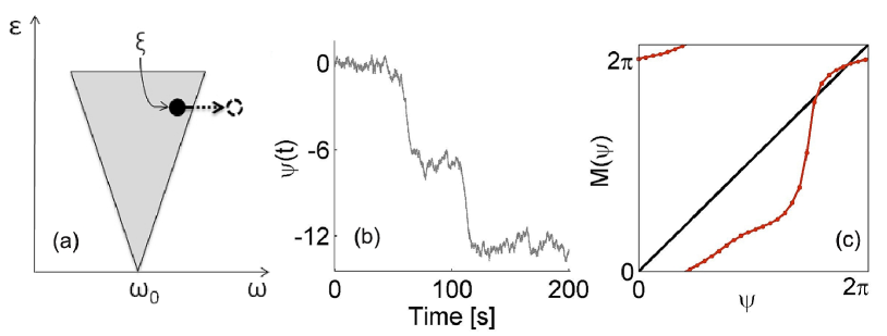
Figure 1: Synchronization discrimination for the coupled phase oscillators (1) with: $\omega_{1}=1.2$, $\omega_{2}=0.8$, $\varepsilon_{1}=0.1$, $\varepsilon_{2}=0.35$, $f_{i}(\phi_{i})=0$, $g_{1}=\sin(\phi_{2}-\phi_{1})$, $g_{2}=\sin(\phi_{1}-\phi_{2})$, and noise strengths $E_{11}=E_{22}=2$. (a) Schematic Arnold tongue to illustrate synchronization Arn . (b) Phase difference, exhibiting two phase slips. (c) Map of $M(\psi_{e})$ for (b) demonstrating that a root of $M(\psi)=\psi$ exists, i.e. that the state is in fact synchronized.

From the inferred parameters of the base functions $f_{i}(\phi_{i})$, $g_{i}(\phi_{i},\phi_{j})$, we can reconstruct the specific functional form of the coupling functions $q_{i}(\phi_{i},\phi_{j})$. The novel advantage of this framework is that it allows reconstruction of the time-variability and evolution of such coupling functions. Simple normalization of the inferred coupling parameters yields the inter-oscillator coupling strengths, and thence the directionality index Paluš and Stefanovska (2003); Rosenblum and Pikovsky (2001); Bahraminasab et al. (2008); Jamšek et al. (2010). If $D\in(0,1]$ the first oscillator drives the second ($1\rightarrow 2$), or if $D\in[-1,0)$ otherwise. Note that, although our discussion relates to two oscillators, Eqs. (1)–(4) are also applicable to a network of oscillators. For expanded discussion, technical description and software codes see Duggento (2012).

As a demonstration of how the synchronization detection works, we simulated numerically a pair of coupled, noisy, phase oscillators (1). Bayesian inference followed by examination of the constructed map $M(\psi_{e})$ showed that our approach successfully distinguishes synchronized ($s(c)=1$) from unsynchronized dynamics ($s(c)=0$), i.e. whether the root $M(\psi_{e})=\psi_{e}$ exists or not. To demonstrate the novelty of our method we consider the characteristic case illustrated in Fig. 1. The parameters were such that the oscillators were only just inside the Arnold tongue so that, for moderate noise, phase slips occurred, as shown schematically in Fig. 1(a). The application of earlier methods based on the statistics of the phase difference Tass et al. (1998); Mormann et al. (2000); Schelter et al. (2006) suggests that the oscillators are not synchronized. In contrast, our new technique shows that the oscillators are intrinsically synchronized as shown in Fig. 1(c): the phase slips are attributable purely to noise (the intensity of which is inferred in matrix $E_{i,j}$), and not to deterministic interactions between the oscillators.

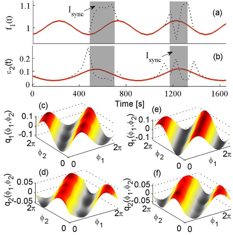
Figure 2: Extraction of time-varying parameters, synchronization and coupling functions from numerical data created by (5). The plots show the results inferred for the numerical values of constants listed in the text. The frequency $f_{1}(t)$ and coupling $\varepsilon_{2}(t)$ are independently varied: (a) $\omega_{1}(t)=\omega_{1}+\tilde{A}_{1}\sin({\tilde{\omega}_{1}}t)$; (b) $\varepsilon_{2}(t)=\varepsilon_{2}+\tilde{A}_{2}\sin({\tilde{\omega}_{2}}t)$. The dotted and full lines plot the parameters when the two oscillators are synchronized for part of the time ($\varepsilon_{1}=0.3$), and not synchronized at all ($\varepsilon_{1}=0.1$), respectively. The regions of synchronization, found by calculation of the synchronization index, are indicated by the gray shaded regions. (c)–(f) show the coupling functions $q_{1}(\phi_{1},\phi_{2})$ and $q_{2}(\phi_{1},\phi_{2})$ for time windows centered at different times: (c) and (d) at $t=350s$; (e) and (f) at $t=1000s$. The window length $t_{w}=50s$, and $\varepsilon_{1}=0.1$ in both cases. Note the similarity in forms of (c) and (e), and of (d) and (f). The other parameters were: $\varepsilon_{2}=0.1$, $\omega_{1}=2\pi 1$, $\omega_{2}=2\pi 1.14$, $\tilde{A}_{1}=0.2$, $\tilde{A}_{2}=0.13$, $\tilde{\omega}_{1}=2\pi 0.002$, $\tilde{\omega}_{2}=2\pi 0.0014$ and noise $E_{11}=E_{22}=0.1$. The phases were estimated as $\phi_{i}=\arctan(y_{i}/x_{i})$.

To see how the new method can also follow time-variations of the parameters, coupling functions and synchronization, we take as an example two coupled noisy Poincaré oscillators:

$$\dot{x}_{i} =-(\sqrt{x_{i}^{2}+y_{i}^{2}}-1)x_{i}-\omega_{i}(t)y_{i}+\varepsilon_{i}(t)(x_{j}-x_{i})+\xi_{i}(t)$$

$$\dot{y}_{i} =-(\sqrt{x_{i}^{2}+y_{i}^{2}}-1)y_{i}+\omega_{i}(t)x_{i}+\varepsilon_{i}(t)(y_{j}-y_{i})+\xi_{i}(t)$$

$$\text{with}\,i=1,2;\,j=1,2;\,i\neq j\,.$$ (5)

We consider bidirectional coupling (1$\leftrightarrow$2), where the natural frequency of the first oscillator, and its coupling strength to the second one, vary periodically. For $\varepsilon_{1}=0.1$ there is no synchronization: the time-varying parameters ($f_{1}(t)$ and $\varepsilon_{2}(t)$) are accurately traced (full red lines of Fig. 2(a) and (b)). For a coupling of $\varepsilon_{1}=0.3$ the two oscillators will be synchronized for part of the time, resulting in intermittent synchronization. The time-variability of the parameters in the non-synchronized intervals is again determined correctly whereas, within the synchronized intervals, the inferred parameters (dashed lines in (a), (b)) diverge from their true values (full red curves). Within these synchronized intervals, all of the base functions are highly correlated, with values lying within the Arnold tongue. The latter was detected as the range for which $s(c)=1$, grey-shaded in Figs. 2(a) and (b).

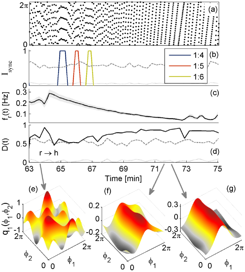
Figure 3: Synchronization, directionality and coupling functions in the cardio-respiratory interaction. (a) Standard 1:$N$ synchrogram. (b) Synchronization index for ratios 1:4, 1:5 and 1:6, as indicated. The light-gray dotted line represents the mean, and the dark-gray dashed line the mean +2 SD, of synchronization indices calculated from 100 surrogate Schreiber and Schmitz (1996) realizations. (c) The time-varying respiration frequency (note the downward ramp due to pacing). The gray areas in (c) represent $\pm$2 SD from the mean value. (d) Directionality index (full curve); the light-gray dotted line represents the mean directionality index calculated from 100 surrogate realizations, and the dark-gray dashed line represents the mean +2 SD. (e)-(g) coupling functions $q_{1}(\phi_{1},\phi_{2})$ calculated at different times, as indicated by the grey arrows.

The reconstructed sine-like functions $q_{1}(\phi_{1},\phi_{2})$ and $q_{2}(\phi_{1},\phi_{2})$ are shown in Figs. 2(c) and (d) for the first and second oscillators, respectively. They describe the functional form of the interactions between the two Poincaré systems (5). The results suggest that the form of the coupling functions does not evolve with time: $q_{1}$ and $q_{2}$, evaluated for later time segments, are presented in Figs. 2 (e) and (f) respectively. By comparison of Figs. 2(c) and (e), or of Figs. 2(d) and (f), we see that the coupling functions did not change qualitatively, even though there were time-varying parameters and weak effects from the noise.

It is well known that modulation and time-variations tend to affect synchronization between biological oscillators Lotrič and Stefanovska (2000); Shiogai et al. (2010); Lewis et al. (2000). Hence the need for a technique able, not only to identify time-varying dynamics, but also to evaluate measures of interaction, e.g. synchronization, directionality and coupling functions. To demonstrate the method on real biological data, we analyzed cardio-respiratory measurements from resting human subjects whose paced respiration was ramped down with decreasing frequency. The instantaneous cardiac phase was estimated by wavelet synchrosqueezed decomposition Daubechies et al. (2011) of the ECG signal. Similarly, the respiratory protophase was extracted from the CO₂ concentration signal, followed by transformation Kralemann et al. (2007) to the phase. The results are shown in Fig. 3. First, just for comparison, the corresponding synchrogram Pikovsky et al. (2001) of the same data is presented in (a). The time-variation of the respiration frequency is clearly evident in (c). By normalizing the inferred coupling parameters, we determined the net directionality of the interactions. Fig. 3(d) suggests that the degree of directionality is time-varying; the analyses confirm that respiration-to-heart is dominant Shiogai et al. (2010); Paluš and Stefanovska (2003); Rosenblum and Pikovsky (2001); Bahraminasab et al. (2008); Jamšek et al. (2010), even for non-paced respiration (not shown). The set of inferred parameters and how they are correlated can be used to determine whether cardiorespiratory synchronization exists and, if so, in what ratio. Fig. 3(b) shows transitions from the non-synchronized to the synchronized state, in ratios 1:4 to 1:5 to 1:6, as the ramp progressed. The cardio-respiratory coupling function, evaluated for three different time windows is presented in Fig. 3(e)-(g). Note that the interactions are now described by complex functions whose form changes qualitatively over time – cf. Fig. 3(e) with (f) and (g). This implies that, in contrast to many systems with time-invariant coupling functions (e.g. Fig. 2(c)–(f) or Daido (1996a, b); Crawford (1995)), the functional relations for the interactions of an open (biological) system can themselves be time-varying processes. By analyzing consecutive time windows, we can even follow the time-evolution of the coupling functions – cf. the similarities i.e. evolution of Figs. 3(f) and (g). It is important to note that the variability in form of the coupling function can cause synchronization transitions. This variability is not caused by the time-varying respiration frequency (which is decomposed separately). We also observed time-evolution of the coupling functions for spontaneous (non-paced) breathing.

In summary, our new method for inference of phase dynamics enables the evolution of a system to be tracked continuously. Unlike earlier methods that only detect the occurrence of transitions to/from synchronization, it reveals details of the phase dynamics, describing the inherent nature of the transitions and simultaneously deducing the characteristics of the noise that stimulated them. We have identified the time-varying nature of the functions that characterize interactions between open oscillatory systems. The cardio-respiratory analysis demonstrated that not only the parameters, but also the functional relationships, can be time-varying, and the new technique follows their evolution effectively. This novel facility immediately invites many new questions, e.g. the functional forms between which the couplings vary, their frequencies of variation, how their variation affects synchronization transitions, and whether there is periodicity or a causal relationship waiting to be identified and understood. Thus a whole new area of investigation has become accessible.

Our grateful thanks are due to Dwain Eckberg for providing the data for Fig. 3, and to M. Arrayas, M.I. Dykman, M. Horvat, D. Iatsenko, P.E. Kloeden, D.G. Luchinsky, R. Mannella, S. Petkoski, and M.G. Rosenblum, for valuable discussions. This work was supported by the Engineering and Physical Sciences Research Council (UK) [grant number EP/100999X1].

References

- Koseska et al. (2010) A. Koseska, E. Ullner, E. Volkov, J. Kurths, and J. Garcia-Ojalvo, J. Theor. Biol. 263, 189 (2010).
- Mondragon-Palomino et al. (2011) O. Mondragon-Palomino, T. Danino, J. Selimkhanov, L. Tsimring, and J. Hasty, Science 333, 1315 (2011).
- Shiogai et al. (2010) Y. Shiogai, A. Stefanovska, and P. V. E. McClintock, Phys. Rep. 488, 51 (2010).
- Marinazzo et al. (2008) D. Marinazzo, M. Pellicoro, and S. Stramaglia, Phys. Rev. Lett. 100, 144103 (2008).
- Barnett et al. (2009) L. Barnett, A. B. Barrett, and A. K. Seth, Phys. Rev. Lett. 103, 238701 (2009).
- Staniek and Lehnertz (2008) M. Staniek and K. Lehnertz, Phys. Rev. Lett. 100, 158101 (2008).
- Hung and Hu (2008) Y. Hung and C. Hu, Phys. Rev. Lett. 101, 244102 (2008).
- Tass et al. (1998) P. Tass, M. G. Rosenblum, J. Weule, J. Kurths, A. Pikovsky, J. Volkmann, A. Schnitzler, and H.-J. Freund, Phys. Rev. Lett. 81, 3291 (1998).
- Mormann et al. (2000) F. Mormann, K. Lehnertz, P. David, and C. E. Elger, Physica D 144, 358 (2000).
- Schelter et al. (2006) B. Schelter, M. Winterhalder, R. Dahlhaus, J. Kurths, and J. Timmer, Phys. Rev. Lett. 96, 208103 (2006).
- Xu et al. (2006) L. M. Xu, Z. Chen, K. Hu, H. E. Stanley, and P. C. Ivanov, Phys. Rev. E 73, 065201 (2006).
- Paluš and Stefanovska (2003) M. Paluš and A. Stefanovska, Phys. Rev. E 67, 055201(R) (2003).
- Rosenblum and Pikovsky (2001) M. G. Rosenblum and A. S. Pikovsky, Phys. Rev. E. 64, 045202 (2001).
- Bahraminasab et al. (2008) A. Bahraminasab, F. Ghasemi, A. Stefanovska, P. V. E. McClintock, and H. Kantz, Phys. Rev. Lett. 100, 084101 (2008).
- Jamšek et al. (2010) J. Jamšek, M. Paluš, and A. Stefanovska, Phys. Rev. E 81, 036207 (2010).
- Galán et al. (2005) R. F. Galán, G. B. Ermentrout, and N. N. Urban, Phys. Rev. Lett. 94, 158101 (2005).
- Kiss et al. (2005) I. Z. Kiss, Y. Zhai, and J. L. Hudson, Phys. Rev. Lett. 94, 248301 (2005).
- Miyazaki and Kinoshita (2006) J. Miyazaki and S. Kinoshita, Phys. Rev. Lett. 96, 194101 (2006).
- Kralemann et al. (2007) B. Kralemann, L. Cimponeriu, M. Rosenblum, A. Pikovsky, and R. Mrowka, Phys. Rev. E 76, 055201 (2007).
- Tokuda et al. (2007) I. T. Tokuda, S. Jain, I. Z. Kiss, and J. L. Hudson, Phys. Rev. Lett. 99, 064101 (2007).
- Levnajić and Pikovsky (2011) Z. Levnajić and A. Pikovsky, Phys. Rev. Lett. 107, 034101 (2011).
- Smelyanskiy et al. (2005) V. N. Smelyanskiy, D. G. Luchinsky, A. Stefanovska, and P. V. E. McClintock, Phys. Rev. Lett. 94, 098101 (2005).
- Friston (2002) K. J. Friston, NeuroImage 16, 513 (2002).
- Sudderth et al. (2010) E. B. Sudderth, A. T. Ihler, M. Isard, W. T. Freeman, and A. S. Willsky, Commun. ACM 53, 95 (2010).
- Luchinsky et al. (2008) D. G. Luchinsky, V. N. Smelyanskiy, A. Duggento, and P. V. E. McClintock, Phys. Rev. E 77, 061105 (2008).
- Duggento et al. (2008) A. Duggento, D. G. Luchinsky, V. N. Smelyanskiy, I. Khovanov, and P. V. E. McClintock, Phys. Rev. E 77, 061106 (2008).
- Penny et al. (2009) W. D. Penny, V. Litvak, L. Fuentemilla, E. Duzel, and K. Friston, J. Neurosci. Methods 183, 19 (2009).
- Pikovsky et al. (2001) A. Pikovsky, M. Rosenblum, and J. Kurths, Synchronization – A Universal Concept in Nonlinear Sciences (Cambridge University Press, Cambridge, 2001).
- (29) Note that the Arnold tongue in this case is considered to be valid for the intrinsic parameters without the effect from the noise. The border of the Arnold tongue from the full dynamics (including the noise) might not be sharp, and can be “blurred” by the noise.
- Schreiber and Schmitz (1996) T. Schreiber and A. Schmitz, Phys. Rev. Lett. 77, 635 (1996).
- Lotrič and Stefanovska (2000) M. B. Lotrič and A. Stefanovska, Physica A 283, 451 (2000).
- Lewis et al. (2000) C. D. Lewis, G. L. Gebber, S. Zhong, P. D. Larsen, and S. M. Barman, J. Neurophysiol. 84, 1157 (2000).
- Daubechies et al. (2011) I. Daubechies, J. Lu, and H. Wu, Appl. and Comput. Harmon. Anal. 30, 243 (2011).
- Daido (1996a) H. Daido, Phys. Rev. Lett. 77, 1406 (1996a).
- Daido (1996b) H. Daido, Physica D: Nonlinear Phenomena 91, 24 (1996b).
- Crawford (1995) J. D. Crawford, Phys. Rev. Lett. 74, 4341 (1995).
- Duggento (2012) A. Duggento, T. Stankovski, P. V. E. McClintock and A. Stefanovska - to be published.