Modelling and Estimation of Covariance of Replicated Modulated Cyclical Time Series

Abstract

This paper introduces the novel class of modulated cyclostationary processes, a class of non-stationary processes exhibiting frequency coupling, and proposes a method of their estimation from repeated trials. Cyclostationary processes also exhibit frequency correlation but have Loève spectra whose support lies only on parallel lines in the dual-frequency plane. Such extremely sparse structure does not adequately represent many biological processes. Thus, we propose a model that, in the time domain, modulates the covariance of cyclostationary processes and consequently broadens their frequency support in the dual-frequency plane. The spectra and the cross-coherence of the proposed modulated cyclostationary process are first estimated using multitaper methods. A shrinkage procedure is then applied to each trial-specific estimate to reduce the estimation risk.

Multiple trials of each series are observed. When combining information across trials, we carefully take into account the bias that may be introduced by phase misalignment and the fact that the Loève spectra and cross-coherence across replicates may only be “similar” – but not necessarily identical – across replicates. The application of the inference methods developed for the modulated cyclostationary model to EEG data also demonstrates that the proposed model captures statistically significant cross-frequency interactions, that ought to be further examined by neuroscientists.

I Introduction

The primary contribution of this paper is a novel model for nonstationary time series that rigorously explains a particular dependence structure in the spectral domain that current models cannot handle. This model is inspired by an electroencephalography (EEG) data set that exhibits coupling between frequency bands. We develop a time-domain representation of the model and derive the corresponding Loève spectrum that captures the desired features. Methods for estimating such features are proposed, and challenges inherent in the estimation discussed.

Nonstationary processes are ubiquitous in practical applications, we mention for example vibratory signals [1, 2], free-drifting oceanic instruments [3], and various neuroscientific applications [4, 5]. Under stationarity, there are several procedures available for obtaining mean-squared consistent estimates of the spectrum. When the assumption of stationarity is rendered invalid, this implies that the second-order structure of the process is usually more complicated. For example, in the case of harmonizable processes, the spectrum is now defined on a dual-frequency plane $(-\frac{1}{2},\frac{1}{2})\times(-\frac{1}{2},\frac{1}{2})$ – in contrast to just the interval $(-\frac{1}{2},\frac{1}{2})$ used in the stationary case. Thus, alternative assumptions need to be made to enable estimation, because it is generally not possible to estimate the Loève spectrum at the ${\cal O}(T^{2})$ pairs of the fundamental Fourier frequencies from time series of length $T$ without imposing additional constraints.

Many models for non-stationary processes have been developed. In classical signal processing, the evolutionary behavior of the spectrum is modeled assuming substantial smoothness in the form of the time-variation of the process, see e.g., [6, 7]. These models form the backbone of using the popular windowed Fourier analysis which implicitly assumes that the signal is approximately stationary within the time window of analysis and that the spectrum of the time series is also smooth within the same window. If the smoothness assumption is not suitable, then replicates of the series are necessary to enable estimation. Unfortunately, in order for replication to be successfully utilized in the estimation, we must have time sample replicates that exhibit both perfect time alignment and exactly the same form of nonstationarity across replicates.

In this paper, we propose an analysis framework that is valid for replicated time series (which is fairly typical in designed experiments) where we repeatedly observe phenomena that are “similar” across replicates but not necessarily identical, and the model must include various realistic features of the replication. First, there may be phase-shifts between the replicates which can complicate the estimation of the Loève spectrum (or the coherency). Second, the dependence between a fixed pair of frequencies (or frequency bands) may not perfectly replicate at each trial. Hence, our model must account for this variation and our estimation methods must have the ability to recover this variation. In Section II, we shall discuss second order modeling of a time series and then focus on frequency correlation descriptions of the signal in Section II-A.

In order to fully understand the underlying stochastic process that produces the observed time series, it is important to develop time domain models that yield the features or shapes that we observe in the frequency domain. In analyzing our electronencephalogram (EEG) data, we observe spectral domain structures that are in parts reminiscent of existing models – e.g. cyclostationary models [8, 9, 10] – e.g. that have a baseline frequency of importance and where harmonics with this period may correlate. However, the structures that we observe do not exactly fit the current models because they show a significant spread in the dual-frequency plane. Thus, motivated by the results from a preliminary analysis of the EEGs, we introduce a time domain class of processes that may reproduce such structure. In Section II-C, we develop the proposed modulated cyclostationary process and discuss its relationship to modulated oscillations, see e.g. Voelcker [11]. Properties of the replication are explicitly discussed in Section II-D.

Guided by the features of spread in dual-frequency and the variation and similarity across replicated trials, we develop an appropriate algorithm for estimation in Section III. First, as suggested by the data, we assume some smoothness of the covariance of the process in frequency to form a replicate-specific estimate of the Loève spectrum. We shall also examine the validity of this assumption in Section III-A. One possibility would be to compute the average spectrum across the replicates after denoising (testing for non-zero contribution) and then perform other linear analysis steps across replicates. These steps are described and discussed in Section III-B.

It is critical to understand the family of Loève coherence functions (or matrices sampled at a set of frequencies and collected in a vector). To explain and recover the possible structures present in these matrices, we could perform a singular value decomposition directly on the estimated matrices derived from each replicate. However, it is not a good idea to apply simple linear methods to the raw Loève spectra because of phase shifts between replicates that will act antagonistically, as is discussed explicitly in Section III-C. Instead we threshold each replicate-specific estimated Loève spectrum on its magnitude. We take account of the Hermitian symmetry of the spectrum as redundant tests makes the testing procedure deteriorate and additionally remove the frequencies that are known to contain unimportant neuroscientific information. Very few of the singular vectors are important to the family of matrices and we can recognize a family of possible structures. This provides a satisfactory description of the variability in frequency across the replicates. Finally, to arrive at a good understanding of a “population” of ”similar” processes across replicates (rather than a trial-specific process), we must carefully consider the sequential ordering of the replicates. As the true underlying Loève coherence might have evolved over the course of the experiment, we anticipate the estimated Loève coherence to also follow a similar behavior. Moreover, it is reasonable to assume that the true Loève coherence is slowly changing throughout the duration of the experiment and thus we anticipate the Loève coherence to be similar between “neighboring” replicates. We discuss this structure and use clustering methods to determine its form.

We conclude by analyzing neuroscientific data with the characteristic of the models developed in this paper. Our choice of EEG data example motivated our development of the model-class of modulated cyclostationary process. EEGs have been important tools in clinical research to investigate underlying brain processes. This particular visual motor EEG data set has been analyzed by others using classical spectral methods: e.g., Freyermuth et al. (2010) developed a wavelets mixed effects model to estimate both the condition-specific spectra and variation in the brain responses across trials; and Fiecas et al. (2011) explored the brain effective connectivity structure in a network of 12 channels using generalized shrinkage methods for estimating classical partial coherence. Here, we demonstrate that the previous analyses missed very interesting oscillatory features – specifically the coupling between the alpha and beta oscillations – that we believe ought to be investigated by neuroscientists. We conclude by discussing how to encompass additional observed features in the model and put forth possible physical interpretations of the observed phenomena.

II Second-Order Modelling

We shall discuss the analysis of the covariance of a zero-mean time series $X_{t}$. We shall therefore model the dual-time autocovariance function [12] of $X_{t}$ given by

$$s(t,l)=\mathrm{Cov}\left[X_{t},X_{t-l}\right]=\mathrm{E}\left[X_{t}X_{t-l}\right].$$ (1)

If $X_{t}$ is second-order stationary then $s(t,l)$ takes the simpler form $\widetilde{s}(|l|)$. It is convenient [13] to represent $X_{t}$ in the frequency domain and one can write down the Cramér representation to be

$$X_{t}=\int_{-\frac{1}{2}}^{\frac{1}{2}}\exp(i2\pi ft)dZ(f),$$ (2)

where $\{dZ(f)\}$ is a zero-mean orthogonal increments process with variance ${\mathrm{Var}}\{dZ(f)\}=S(f,f)\,df$ if the process has a smooth spectrum. If we define the Fourier transform of $\widetilde{s}(|l|)$ to be $\widetilde{S}(f)$, then for stationary processes $S(f,f)\equiv\widetilde{S}(f)$. The total “energy” or variance of $X_{t}$ admits a representation of integrating $S(f,f)$ over all $f$. Therefore, if a given frequency $f$ has a relatively large value of $S(f,f)$ associated with it, then we say that oscillations of frequency $f$ dominate the signal. Furthermore the autocovariance sequence of a stationary process is a Fourier transform pair with the spectrum. Therefore the spectrum fully represents a Gaussian time series because series are fully specified by their autocovariance sequence. While useful in a general setting and the focus of several studies, the stationarity assumption is not valid for many forms of data. We now outline how the representation of a stationary covariance can be generalized to a larger class of processes that can capture realistic features.

II-A Dual-frequency representation of Covariance

As noted, EEG signals are characterized in terms of their frequency content. While the spectrum already tells us a great deal about the presence of oscillatory patterns and behavior, it does not capture other interesting and more complex oscillatory properties of these signals, such as the dependence of the coefficients across the Fourier frequencies. In general, for non-stationary signals, such correlations are present, even if impossible for stationary signals and are important to characterize. It is therefore necessary to define a measure of the degree of correlation between the increment process at two different frequencies. For this purpose, we use the Loève coherence (a measure of the covariance) using the formalism of harmonizable processes [14]. A time series $X_{t}$ belongs to the harmonizable class if it has the Cramér-Loève representation

$$X_{t}=\int_{-\frac{1}{2}}^{\frac{1}{2}}\exp(2\pi ift)dZ(f),$$ (3)

where the increment random process $dZ(f)$ still has zero-mean but also satisfies

$$\mathrm{Cov}[dZ(f_{1}),dZ(f_{2})]=\mathrm{E}[dZ(f_{1})dZ^{\ast}(f_{2})]=S(f_{1},f_{2})df_{1}df_{2},$$

where $dZ^{\ast}(f)$ denotes the complex-conjugate of $dZ(f)$ and $S(f_{1},f_{2})$ is a complex-valued scalar quantity called the Loève spectrum [12]. It may appear that Equation (2) strongly resembles Equation (3) in form, but the introduction of the correlations between frequencies significantly modifies the appearance of realizations $\{X_{t}\}$. The Loève spectrum easily relates to the primary quantity of the auto-covariance of $X_{t}$ from the following relationship

$$s(t,l)=\mathrm{cov}[X_{t},X_{t-l}]=\int_{-\frac{1}{2}}^{\frac{1}{2}}\int_{-\frac{1}{2}}^{\frac{1}{2}}S(f_{1},f_{2})e^{2i\pi[(f_{1}-f_{2})t+f_{2}l]}\,df_{1}\,df_{2}.$$ (4)

Thus, the covariance of $X_{t}$ with $X_{t-l}$ across time $t$ is still decomposed to contributions across frequency. However, in general, we also need to consider the cross-dependencies between different frequencies.

The Loève coherency at the pair of frequencies $(f_{1},f_{2})$, denoted $\tau(f_{1},f_{2})$, is defined to be

$$\tau(f_{1},f_{2})=\frac{S(f_{1},f_{2})}{\sqrt{S(f_{1},f_{1})S(f_{2},f_{2})}}=\rho^{1/2}(f_{1},f_{2})e^{-i\phi(f_{1},f_{2})},$$ (5)

where the Loève coherence at $(f_{1},f_{2})$ is $\rho(f_{1},f_{2})=\left|\tau(f_{1},f_{2})\right|^{2}$, and the Loève coherency phase is $\phi(f_{1},f_{2})$. The Loève coherence values lie in the range $[0,1]$ where values closer to $1$ indicate a stronger linear dependence between the random coefficients $dZ(f_{1})$ and $dZ(f_{2})$. It can also be interpreted as the proportion variance of $dZ(f_{1})$ that is explained by a linear relationship to $dZ(f_{2})$, e.g.

$$dZ(f_{1})=\tau dZ(f_{2})+\varepsilon(f_{1},f_{2}).$$ (6)

where $\varepsilon(f_{1},f_{2})$ is uncorrelated with $dZ(f_{2})$. When the Loève coherence is close to $1$, one interpretation is that increased oscillatory activity at the $f_{1}$ frequency band is strongly associated with an excitation (or an inhibition) of oscillatory activity at the $f_{2}$ band. When $|\tau|<1$ then the interpretation of Equation (6) is that the variance of $dZ(f_{1})$ is “partially explained” by $dZ(f_{2})$. Some care must be applied, because the complete relationship between two complex-valued quantities may be widely-linear rather than linear, see. e.g. [12, Eqn. 12], and the full set of relationships takes the (widely linear) form of

$$dZ(f_{1})=\tau dZ(f_{2})+\zeta dZ^{\ast}(f_{2})+\varepsilon(f_{1},f_{2}),$$ (7)

where $\varepsilon(f_{1},f_{2})$ is both uncorrelated to and has zero relation with $dZ(f_{2})$. Because $dZ^{\ast}(f_{2})\equiv dZ(-f_{2})$ we can take this extra information into account by considering the correlation between the full set of frequencies (e.g. also positive frequencies with negative frequencies) when analyzing $dZ(f)$, rather than calculating the Loève coherence of $dZ(f)$ and $dZ^{\ast}(f^{\prime})$ and the complementary Loève coherence over a restricted set of frequencies.

Having extended the classical spectrum to the Loève spectrum (with particular characteristic features) we will now need to develop inference methods for this scenario. There are two natural sets of assumptions one can make concerning the Loève spectrum. First, one can assume $S(f_{1},f_{2})$ to be a smooth function of $f_{1}$ and $f_{2}$ and adapt statistical procedures from non-parametric function estimation. Second, one can impose some form of sparsity on the support of $S(f_{1},f_{2})$ – e.g., assume that the support of $S(f_{1},f_{2})$ is only a set of lines in the dual-frequency domain [15, 16] which is the case if the process is cyclostationary [9, 10]. Of course, our model assumptions should be as realistic as possible and must closely match the data being analyzed. Our motivation for these methods are features encountered in neuroscience, but we envision their application to be more generic to processes exhibiting strong harmonics such as (bio-)acoustic signals. In Figure 1, we see these features where the raw non-parametric estimates of the Loève spectrum with limited smoothing have periodic components that display time-variation and some “broadening” which is a deviation from crisply-defined spectral lines obtained from the class of cyclostationary processes. Some care should be taken when interpreting these figures, as when averaging over trials we are getting “sample characteristics” over the full mixture existing in the population of matrices over the population, a topic we shall revisit.

(a)

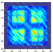
(b)

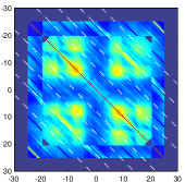
(c)

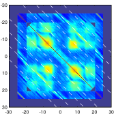
Figure 1: Each plot is the square root of the Loève coherence averaged across separate blocks of 20 trials. The $x$ and $y$ axes are for frequencies in the range $(-30,30)$ Hertz. Plot (a) corresponds to trials 1–20; Plot (b) corresponds to trials 41–60; Plot (c) corresponds to trials 81–100. These patterns are highly replicable across the aggregate trials.

II-B Brief Review of Cyclostationary Processes

We first discuss the model structures that will allow us to describe correlations in frequency like in Figure 1. Firstly, there is structure consistent with support on lines parallel to the diagonal. The simplest such process is a cyclostationary process (see e.g. [9]). The covariance of cyclostationary process repeats perfectly in time over a cyclical period of $D>0$, say. In fact the Loève spectrum of a cyclostationary process takes the form (see e.g. [8, 17]) for some integer value $C\geq 1$

$$S(f_{1},f_{2})=\sum_{c=-C}^{C}S_{c}(f_{2})\delta\left(f_{1}-f_{2}-\frac{c}{D}\right),$$ (8)

where $\{S_{c}(f)\}$ are $2C+1$ functions defined for $f\in[-1/2,1/2]$, with respective inverse Fourier transforms $s_{c}(l)$. The sum in (8) must be symmetric in $c$ as the observed process $X_{t}$ is real-valued. This Loève spectrum is equivalent to a time domain covariance of

$$s(t,l)=\int_{-\frac{1}{2}}^{\frac{1}{2}}\int_{-\frac{1}{2}-f}^{\frac{1}{2}-f}S(f+\nu,f)e^{2i\pi(\nu t+fl)}\,d\nu\,df=\int_{-\frac{1}{2}}^{\frac{1}{2}}\sum_{c=-C}^{C}S_{c}(f)e^{2i\pi(\frac{c}{D}t+fl)}\,df=\sum_{c=-C}^{C}s_{c}(l)e^{2i\pi\frac{c}{D}t},$$ (9)

where $\varsigma_{c}(t,l)=s_{c}(l)e^{2i\pi\frac{c}{D}t}$ and each contribution to the covariance $\{\varsigma_{c}(t,l)\}$ has associated period $D/c$, and where each contribution represents a line in the Loève spectrum, spaced at $c/D$ from the diagonal.

To understand how line components aggregate in the representation, consider the example

$$X_{t} = \epsilon_{t}+a(f^{\prime})\cos(2\pi f^{\prime}t+\phi_{0}(f^{\prime}))\epsilon_{t}+a(2f^{\prime})\cos(2\pi 2f^{\prime}t+\phi_{0}(2f^{\prime}))\epsilon_{t}$$ (10)

which is a twice-modulated stationary process $\epsilon_{t}$. Then, the Loève spectrum of $X_{t}$ has contributions at $f_{1}=f_{2}$ and $f_{1}-f_{2}=\pm cf^{\prime}$. If the spectrum of $\epsilon_{t}$, denoted $S_{\epsilon}(f,f)$, exhibits a peak at $f^{\prime},$ then this peak generates a whole structure from the modulation of several peaks. See Figure 2(a), which illustrates how one peak in the stationary process is propagated onto several points by the modulation, where the ${\mathcal{S}}_{c}(f_{1},f^{\prime})$ are determined by the spectrum of $\epsilon_{t}$ and the amplitudes $a(f^{\prime})$ and phases $\phi(f^{\prime})$ and so on. The linear mechanism of Equation (10) mimics the behaviour of non-linear systems of coupled oscillations, see for example the full discussion in [18, pp. 25]. However, while the cyclostationary model allows us to understand the mechanisms of the second order structure of non-linear models with coupled oscillations, and describes the “skeleton” of the features present in the EEG data, it is not sufficient to describe the covariance properties of the observed data in more detail, as evidenced from Figure 3(a) and (c) showing individual trial estimated Loève coherences.

II-C Modulated Cyclostationary Processes

We now develop the novel class of modulated cyclostationary processes. In doing so, we wish to retain the assumption of simplicity of the Loève spectrum but do not constrain the true geometry of the spectrum to live on the exact lines as in cyclostationary process. Hence, we relax Equation (9) to

$$s(t,l) = \sum_{c=-C}^{C}\varsigma_{c}(t,l)=\sum_{c=-C}^{C}a_{c}(t)s_{c}(l)e^{2i\pi tc/D}.$$ (11)

This covariance is nearly identical to Equation (9) but now each line contribution in the covariance has been modulated by the time-varying amplitude $a_{c}(t)$.

This is very similar to the notion of uniformly modulated processes; see e.g. [18] but acting on the components of the covariance sequence of the process, each component being shifted in frequency by $c/D$. Therefore, unlike uniformly modulated processes, here we allow each extra line to be modulated differently. The combination of these actions is a generalization of the uniformly modulated processes. The reason for this is two-fold. First, we are modulating each spectral correlation component $\{s_{c}(l)\}$ using a different function, and so our process cannot necessarily be written in the form $X_{t}=\sigma(t)\eta(t)$ where $\eta(t)$ is a cyclostationary process. Second, even if each $s_{c}(l)$ is modulated in an identical manner, the corresponding $\eta(t)$ is not stationary but cyclostationary.

Some care also needs to be used in designing the modulating functions $\{a_{c}(t)\}$. The diagonal structure in the Loève spectrum is preserved as broadened lines only if $a_{c}(t)$ is varying more slowly compared to the oscillation $e^{2i\pi tc/D}$. Otherwise, the diagonal lines will appear as “shifted” in frequency. One option would be to constrain the support of the Fourier transform of $a_{c}(t)$ so that it is sufficiently well within $-c/D$ and $c/D$. This constraint is often encountered in signal processing when modeling an amplitude varying oscillation giving rise to a signal that is strongly related to the types of processes that we wish to describe, see e.g. the common constraints put on amplitudes in Bedrosian’s theorem [19]. In addition to amplitude modulation, it would also be natural in some scenarios to include frequency modulation and replace $a_{c}(t)$ by $a_{c}(t)e^{i\varphi_{c}(t)}$ in Equation (11). Care would have to be taken to keep the average modulation moderate, e.g. $\int a_{c}^{2}(t)\varphi_{c}^{\prime}(t)dt/\int a_{c}^{2}(t^{\prime})dt^{\prime}\approx 0$, as otherwise the process changes characteristics. We investigate this further in the examples in Section IV.

We find that the Loève spectrum is then an aggregation of $2C+1$ components taking the form

$$S_{c}(f+\nu,f) = \sum_{t,l}\varsigma_{c}(t,l)e^{2i\pi(t\nu+lf)}=\sum_{t,l}s_{c}(l)a_{c}(t)e^{-2i\pi tc/D}e^{2i\pi(t\nu+lf)}=S_{c}(f)A_{c}(\nu-\frac{c}{D}).$$ (12)

Comparing Equation (8) to Equation (12), we see the difference between the modulated and the standard cyclostationary model: the multiplication with the amplitude function $a_{c}(t)$ in Equation (12) will yield a broadening of lines centered at $\nu=c/D$, with a potential asymmetry around the line dependent on the form of $A_{c}(\cdot)$. See Figure 3(c) for an example of the Loève spectrum estimated from real data and also a synthetic example in Figure 2(d) with the associated modulating function $a_{c}(t)$ in Figure 2(c). Note that the variance across many near lying oscillations will broaden the populations of oscillations even further, a feature which is consistent with our trial averages. From the Heisenberg-Gabor principle (see e.g. [18, p. 151]), when $a_{c}(t)$ is more transient in time, then the Loève spectrum is broader or more dispersed in frequency. Thus, if a signal displays a very brief temporal response, then the response will be very diffuse in dual-frequency. In addition, as noted, we could introduce frequency modulation to Eqn (12) by replacing $a_{c}(t)$ by $a_{c}(t)e^{-i\varphi_{c}(t)},$ as long as $|\varphi_{c}^{\prime}(t)|$ is constrained not to shift the mean frequency.

To connect our results more generally with amplitude and frequency modulated signals more strongly, let $U_{t}$ be a zero mean stationary signal and take $K/2$ to be a positive-valued integer so that

$$X_{t}=\sum_{k=-K/2}^{K/2}\alpha_{k}(t)e^{2i\pi kt/D}U_{t},$$ (13)

where $U_{t}$ is a stationary process with autocovariance sequence $\tilde{s}(l)$. Then

$$\mathrm{cov}\left\{X_{t},X_{t-l}\right\} = \sum_{k=-K/2}^{K/2}\sum_{k^{\prime}=-K/2}^{K/2}\alpha_{k}(t)e^{i2\pi kt/D}\alpha_{k^{\prime}}(t-l)e^{-i2\pi k^{\prime}(t-l)/D}\tilde{s}(l)$$

$$= \sum_{c=-K}^{K}\sum_{v=-K/2+c}^{K/2+c}\alpha_{c+v}(t)\alpha_{v}(t-l)e^{i(2\pi(c+v)t/D-2\pi v(t-l)/D)}\tilde{s}(l).$$

For transparency of expression we investigate a simplified case and let $\alpha_{k}(t)=\alpha_{k}\alpha(t)$ for $k=-K/2,\dots,K/2$, and this implies that the form of the covariance takes the simpler form of

$$\mathrm{cov}\left\{X_{t},X_{t-l}\right\} = \sum_{c=-K}^{K}\alpha(t)\alpha(t-l)e^{2i\pi ct/D}\sum_{v=-K/2+c}^{K/2+c}\alpha_{c+v}\alpha_{v}e^{i2\pi vl/D}\tilde{s}(l).$$

To further simplify the covariance we define an additional function $s_{c}(l)$ and find that

$$\mathrm{cov}\left\{X_{t},X_{t-l}\right\} \approx \sum_{c=-K}^{K}\alpha^{2}(t)e^{2i\pi ct/D}s_{c}(l),\quad s_{c}(l)=\sum_{v=-K/2+c}^{K/2+c}\alpha_{c+v}\alpha_{v}e^{i2\pi vl/D}\tilde{s}(l),$$

as long as $\alpha(t)$ is not too variable. Thus we see a simple path to approximate generation of signals with the desired characteristics.

(a)

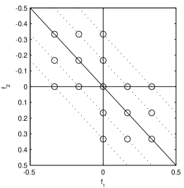
(b)

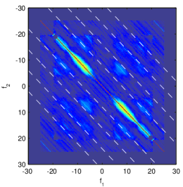
(c)

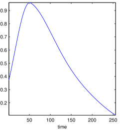
(d)

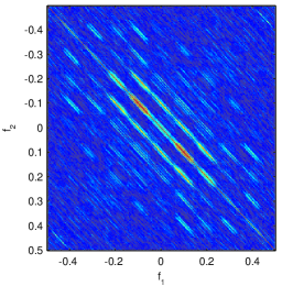
Figure 2: Plot (a) illustrates that by giving a $\delta$ contribution to the spectrum at frequency $f^{\prime}=\pm 1/6$ the cyclostationary multiplication leads to a plethora of contributions across the dual-frequency plane. Plot (b) is the average of cross Loève coherences for the real data over 20 trials. Plot (c) is the within trial modulation function for a simulated example. Plot (d) is the average cross-coherence of a uniformly modulated cyclostationary process over 20 simulated data.

II-D Replicated Modulated Cyclostationary Processes

We have proposed a new class of modulated cyclostationary processes. Now, if we repeatedly observe signals as realizations of a process, we need to understand the precise notion of replication in the data generating scheme. For each replicate $r$, we shall assume that the length of the time series is $T$ and denote the random vector for the $r$-th replicate to be ${\mathbf{X}}^{(r)}=\begin{pmatrix}X_{1+(r-1)T}&\dots&X_{rT}\end{pmatrix}$. It is reasonable to assume the probability density function of ${\mathbf{X}}^{(r)}$ to be from some mixture

$$p\left({\mathbf{X}}^{(r)}\right)=\sum_{m=1}^{M}\pi^{(rm)}p_{rm}\left({\mathbf{X}}^{(r)}\right),$$ (14)

that is, the distribution is a mixture between $M$ different states, and where naturally $\sum_{m}\pi^{(rm)}=1$ for any replicate $r$. As a first step, we shall assume that the $M$ densities $\{p_{rm}\left(\cdot\right)\}$ in Equation (14) are Gaussian. However, we shall be a bit careful in modeling other aspects of $p_{rm}\left(\cdot\right)$. In many related problems one would usually take $p_{rm}\left(\cdot\right)=p_{m}\left(\cdot\right)$. However, this constraint is too stringent and would fail under non-stationarity because time-shifts and phase-shifts fundamentally change the distribution between replicates, and some $r$-dependence must be inserted back into the model. Here, both a replicate-specific overall time-shift $\delta^{(r)}$ and between component phase shifts $\phi_{c}^{(r)}$ will be needed. We shall also permit amplitude modulation per component given by $\theta^{(r)}_{c}$. We can think of $\delta^{(r)}$ as “synchronizing” the whole waveform observed in ${\mathbf{X}}^{(r)}$, while $\phi_{c}^{(r)}$ “synchronizes” the harmonic components present in ${\mathbf{X}}^{(r)}$, vis-a-vis each other.

Then using the newly introduced parameters, we model the common covariance in the replicated $r$ when mixture $m$ only is present as

$$s^{(rm)}(t,l) = \sum_{c=-C_{m}}^{C_{m}}\varpi_{c}^{(rm)}(t,l)=\sum_{c=-C_{m}}^{C_{m}}\theta^{(r)}_{c}a_{c}^{(m)}(t-\delta^{(r)})s_{c}^{(m)}(l)e^{2i\pi tc/D+i\phi_{c}^{(r)}},$$ (15)

where by necessity $\phi_{0}^{(r)}=0$, $\theta^{(r)}_{c}\geq 0$ and $\phi_{c}^{(r)}\in\left(-\pi,\pi\right]$. This model may seem somewhat clumsy but each symbol is directly modulating an aspect of the covariance. With this we find that the covariance in frequency is given by

$$S^{(rm)}(f+\nu,f) = \sum_{c=-C_{m}}^{C_{m}}S_{c}^{(m)}(f)A_{c}^{(m)}(\nu-\frac{c}{D})\theta^{(r)}_{c}e^{i\phi_{c}^{(r)}+2i\pi(\nu-\frac{c}{D})\delta^{(r)}}.$$ (16)

We therefore determine that the covariance of the increment random process $\{dZ^{(r)}(f)\}$ for the $r$-th replicate is strongly dependent on the replicate-specific phase-shift $\phi_{c}^{(r)}$, the time shift $\delta^{(r)}$, and the amplitude modulation $\theta^{(r)}_{c}$. The function $A_{c}(\cdot)$ will still cause “blurring” in frequency and instead of the $\delta$- function localization of Eqn (8) we shall observe spread in dual-frequency. For estimation purposes especially the phase-shift and time-shift in Eqn (16) are problematic as they cause local variability in $S(f+\nu,f)$ and so local non-parametric estimators that smooth may perform badly, and the additional dependence of the time and phase shift are unfortunate. Due to the previously specified locality of $A_{c}^{(m)}(\cdot)$ there will be no substantial overlap in the plane between the different components enumerated by $c$. We can therefore say that

$$\left|S^{(rm)}(f+\nu,f)\right| \approx \sum_{c=-C_{m}}^{C_{m}}\left|S_{c}^{(m)}(f)\right|\left|A_{c}^{(m)}(\nu-\frac{c}{D})\right|\theta^{(r)}_{c}.$$ (17)

Note that the variation in magnitude across replicates is now uniquely captured by the constant $\theta^{(r)}_{c}$. Absolute coherency for the $r$-th replicate using component $m$ near contribution $c$ can then be written as

$$\rho^{1/2}(f_{1},f_{2}) = \frac{\left|S^{(rm)}(f_{1},f_{2})\right|}{\sqrt{\left|S^{(rm)}(f_{1},f_{1})\left|S^{(rm)}(f_{2},f_{2})\right|\right|}}$$

$$= \frac{\left|S_{c}^{(m)}(f_{2})\right|\left|A_{c}^{(m)}(f_{1}-f_{2}-\frac{c}{D})\right|\theta^{(r)}_{c}}{\left|S_{0}^{(m)}(f_{1})\right|^{1/2}\left|S_{0}^{(m)}(f_{2})\right|^{1/2}\left|A_{0}^{(m)}(-\frac{c}{D})\right|\theta^{(r)}_{0}}=\rho^{1/2}_{mc}(f_{1},f_{2})\frac{\theta^{(r)}_{c}}{\theta^{(r)}_{0}},$$

where $\rho^{1/2}_{mc}(f_{1},f_{2})$ is modeled in terms of a basis expansion

$$\rho^{1/2}_{mc}(f_{1},f_{2}) = \sum_{p=1}^{\infty}c_{mcp}\psi_{p}\left(f_{1},f_{2}\right).$$ (18)

The basis $\{\psi_{p}(f_{1},f_{2})\}$ is chosen iteratively to maximize the magnitude of $c_{mcp}$ for each $p$ starting with $p=1$, and so Equation (18) in fact defines $\{\psi_{p}\left(f_{1},f_{2}\right)\}$. Constructing this representation is generally fine as long as the function $\rho^{1/2}(f_{1},f_{2})$ is square integrable. While $\rho^{1/2}_{mc}(f_{1},f_{2})\geq 0$, this is no longer true for the elements in which we do the expansion, e.g. point-wise $\psi_{p}(f_{1},f_{2})$ may be negative, but this should produce no problems. We get that

$$\rho^{1/2}(f_{1},f_{2}) = \sum_{c=-C_{m}}^{C_{m}}\rho^{1/2}_{mc}(f_{1},f_{2})\frac{\theta^{(r)}_{c}}{\theta^{(r)}_{0}}=\sum_{c=-C_{m}}^{C_{m}}\sum_{p=1}^{\infty}\frac{\theta^{(r)}_{c}}{\theta^{(r)}_{0}}c_{mcp}\psi_{p}\left(f_{1},f_{2}\right)=\sum_{p=1}^{\infty}d_{mp}^{(r)}\psi_{p}\left(f_{1},f_{2}\right).$$ (19)

We therefore obtain that the coherency $\rho^{1/2}(f_{1},f_{2})$ for replicate $r$ can be represented in terms of a basis expansion where the weights depend on the trial and the state $m$. As usual $\{\psi_{p}\left(f_{1},f_{2}\right)\}_{p}$ are chosen to be orthonormal.

III Estimation

Having developed a non-parametric model that captures the structures we expect to see in the data, we now develop a procedure for estimating these structures. This is in contrast to statistics, where attention has been focused on very special forms of nonstationary covariance structures, see e.g. [16] and [9]. Having proposed a general non-parametric class of models, we now apply a non-parametric estimation technique. Our philosophy is that by applying non-parametric estimation methods we avoid the bias that is inherently present in parametric models may due to potential omission of features of the data. Ideally once such features have been discovered to be significant they would be put to further scrutiny.

III-A Multitaper (MT) Estimation

Since the covariance structure has been modified by the set of smooth amplitude functions $A_{c}^{(m)}(\cdot)$, it is reasonable to assume that the Loève spectrum is smooth. We therefore need a more general non-parametric estimator, and we turn to [20] and the usage of multitaper estimators to this purpose. We develop a multi-taper procedure for estimating the Loève coherence from several time-aligned brain waves recorded from many trials. Denote $X_{t}^{r}$ to be the time series recorded at the $r$-th trial. Define $h_{t}^{(k)}$ to be the $k$-th orthogonal taper that satisfies $\sum_{t}[h_{t}^{(k)}]^{2}=1$ and $\sum_{t}h_{t}^{(k_{1})}h_{t}^{(k_{2})}=0$ if $k_{1}\neq k_{2}$ (for a discussion of tapers and tapering see e.g. [21]). The $k$-th tapered Fourier coefficient at frequency $f$ is then defined to be

$$x_{k}^{(r)}(f) = \sum_{t}h_{t}^{(k)}X_{t}^{r}\exp(-i2\pi ft),\ \ f\in(-\frac{1}{2},\frac{1}{2}).$$

The $k$-th Loève periodogram at the frequency pair $(f_{1},f_{2})$ is defined to be

$$I_{k}^{(r)}(f_{1},f_{2}) = x_{k}^{(r)}(f_{1})x_{k}^{(r)\ast}(f_{2}),\ \ (f_{1},f_{2})\in(-\frac{1}{2},\frac{1}{2})\times(-\frac{1}{2},\frac{1}{2})$$ (20)

The tapered Loève periodogram estimates can be averaged across tapers to produce a suitable trial-specific non-parametric estimator, the Loève multitaper spectral estimator,

$$\overline{I}^{(r)}_{\cdot}(f_{1},f_{2})=\frac{1}{K}\sum_{k}I_{k}^{(r)}(f_{1},f_{2}).$$ (21)

Note that the expectation of $I_{k}^{(r)}(f_{1},f_{2})$ is not exactly $S(f_{1},f_{2})$ because of the blurring inherent in using tapers. It therefore may seem reasonable to weight the sum in (21) by the eigenvalues of the localization operator that produced the tapers $\{h_{t}^{(k)}\}$, see e.g. [21], but as these are chosen to be so close to unity in most cases, using a plain average of the estimates with a weighting of unity makes little or no difference in practice. To obtain an estimator of the “population” Loève spectrum, we may take the average of the trial-specific estimators and can also estimate the coherency in Equation (5)

$$\overline{I}^{(\cdot)}_{\cdot}(f_{1},f_{2})=\frac{1}{R}\sum_{r}I_{\cdot}^{(r)}(f_{1},f_{2}),\quad\widehat{\tau}^{(r)}(f_{1},f_{2})=\frac{\overline{I}^{(r)}_{\cdot}(f_{1},f_{2})}{\sqrt{I^{(r)}_{\cdot}(f_{1},f_{1})I^{(r)}_{\cdot}(f_{2},f_{2})}}.$$ (22)

Using multitaper methods to estimate the Loève coherency has already been used in Geophysics [22].

Remark. We reiterate that the problem with averaging the Loève periodogram in frequency and trial lies in the variability of the phase (see Equation (16)). For a cyclostationary process, we get a Loève spectrum that is quite variable in phase across replicates and its phase exhibits smooth variation along parallel lines. The magnitude in contrast does not depend on replicate-specific time initialization of the cycles. We believe that over the tapers the estimated phase is stable for a given replicate at a given frequency pair but that there is variability in where in the cycle we “start” across replicates. Averaging phase dependent quantities in a direction perpendicular to the diagonals across trials therefore makes no sense, even if when we average the real and imaginary parts we are producing a magnitude weighted average of the phase, which is clearly an improvement. For this reason Equation (22) is a “less than optimal” summary of the population characteristics of the Loève coherence matrices.

Note that $\overline{I}^{(\cdot)}_{\cdot}(f_{1},f_{2})\in{\mathbb{C}}$ and its imaginary part is non-zero for most pairs $(f_{1},f_{2}$). For a sufficiently large number of tapers $K$, it is reasonable to assume that $\Re\{\overline{I}^{(r)}_{\cdot}(f_{1},f_{2})\}$ and $\Im\{\overline{I}^{(r)}_{\cdot}(f_{1},f_{2})\}$ are nearly jointly Gaussian (see e.g. [23], and [24] for stationary processes). This means that the complex variable $\overline{I}^{(r)}_{\cdot}(f_{1},f_{2})$ is nearly complex-Gaussian (see, e.g., [25, p. 39]). Moreover, when $K$ is sufficiently large and $X_{t}^{(r)}$ is stationary then we argue in the Appendix that for $f_{1}\neq f_{2}$,

$$\widehat{\tau}^{(d)}(f_{1},f_{2})\overset{d}{\approx}N_{C}\left(0,\frac{1}{K}\right),\quad K|\widehat{\tau}^{(d)}(f_{1},f_{2})|^{2}\overset{d}{\approx}\frac{1}{2}\chi^{2}_{2}.$$ (23)

III-B Multitaper-Singular Value Decomposition (MT-SVD)

We have $R$ individual replicate-specific estimates of the square-root coherency $\widehat{\rho}_{r}^{1/2}(f_{1},f_{2})$. Because we need to implement digital processing, we sample the frequency space to $\{\mathbf{f}_{1},\dots,\mathbf{f}_{N}\}={\mathscr{F}}$, where $\mathbf{f}_{n}=(f_{1}^{(n)},f_{2}^{(n)})$ is the $n$-th pair of fundamental frequencies. These frequencies do not necessarily cover the spectrum in the Nyquist range and hence we shall discuss what frequencies to include subsequently. We construct a vector ${\mathbf{p}}^{(r)}=\begin{pmatrix}\widehat{\rho}_{r}^{1/2}(\mathbf{f}_{1})&\dots&\widehat{\rho}_{r}^{1/2}(\mathbf{f}_{N})\end{pmatrix},$ and from the full set of vectors we form

$${\mathbf{P}}^{T}=\begin{pmatrix}{\mathbf{p}}^{(1)T}&,\dots&,{\mathbf{p}}^{(R)T}\end{pmatrix},\quad{\mathbf{P}}={\mathbf{U}}\bm{\Xi}{\mathbf{V}}^{H}=\sum_{k}{\xi}_{k}\mathbf{u}_{k}\mathbf{v}_{k}^{H}.$$ (24)

We can therefore chose to take ${v}_{kn}=\psi_{k}\left(\mathbf{f}_{n}\right),$ and thus expand the matrix in terms of this basis. We would recognize similar shapes in the dual-frequency domain by examining $\{\mathbf{u}_{k}\}.$ Now we do not wish to implement this procedure straight on the raw matrix $\widehat{\mathbf{P}}$ as the sampling characteristics of large matrices will make us “learn noise”. We shall start by determining which part of the matrix is really non-zero.

III-C Thresholded Multitaper-Singular Value Decomposition (TMT-SVD)

We first test whether the Loève spectrum is zero at off-diagonal points $(f_{1},f_{2})$ where $f_{1}\neq f_{2}$, as this will help us shrink the estimates of the coherence for each replicate, and thus remove spurious non-zero coherence. It would be tempting to compare raw coherency across replicates, but we remind the reader of the incoherent phase between replicates, as described by Equation (16). We threshold the individual coherency entries by using the distribution of Equation (23), implementing a conservative False Discovery Rates correction (FDR) [26] to avoid multiple testing issues, but accounting for Hermitian symmetry of the data. This produces ${\mathbf{P}}^{({\mathrm{ht}})}$, from which a singular value decomposition can easily be calculated, resulting in $\mathbf{u}_{k}^{({\mathrm{ht}})}$ (the trial specific vector), $\xi_{k}^{({\mathrm{ht}})}$ (the singular values) and $\mathbf{v}_{k}^{({\mathrm{ht}})}$ (the frequency structure vector). We use $\xi_{k}^{({\mathrm{ht}})}$ to determine how many wave-forms we need to keep in, in order to describe most of the covariance. We use $\mathbf{u}_{k}^{({\mathrm{ht}})}$ as a basis from clustering the trials, using the $k$-means method [27].

IV EEG Example

Overview of the EEG Analysis. Brain patterns operate at given ranges of frequencies (see [13]). Most studies concern frequencies corresponding to the (i.) delta band (0-4 Hertz) which appears in adult slow wave sleep; (ii.) theta band (4-8 Hertz) which is believed to be associated with the inhibition of elicited responses; (iii.) alpha band (8-12 Hertz) which is present when eyes are closed and is also associated with inhibition control; (iv.) beta band (12-30 Hertz) which is present during alert and active states; (v.) gamma band (30-100 Hertz) which are thought to represent the highly synchronous activity of neurons in response to a specific cognitive or motor function. To examine oscillatory properties of single-channel brain signals, scientists use spectral analysis methods [28] which decompose the covariance of an observed time series according to the independent contributions (weightings or variance) of complex exponentials associated with different frequencies. Empirical analyses of our EEG dataset suggest the existence of coupling or dependence between coefficients at the alpha ($8-12$ Hertz) and beta ($12-30$ Hertz) bands. Such dependence should not be ignored as they could turn out to be important biomarkers for differentiating between different cognitive processes and mental states. While this concept of cross-frequency coherence is potentially powerful, it is not commonly used in practice because of the lack of methods for testing significance of these dependence measures. In this paper, we elucidate on this concept of spectral dependence and use this to further interrogate the visual-motor EEG dataset.

(a)

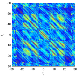
(b)

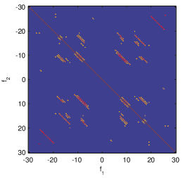
(c)

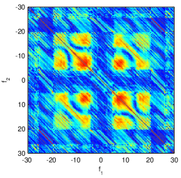
(d)

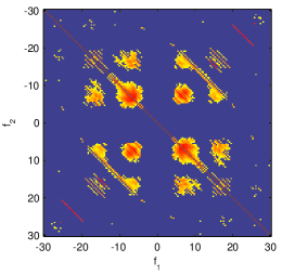
Figure 3: Plots (a) and (c): Two trials of correlations across frequencies showing two types of structure. Plots (b) and (d): Corresponding thresholded versions using FDR (b) and (d). These are trials $b=1$ and $b=8$.

(a)

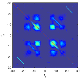
(b)

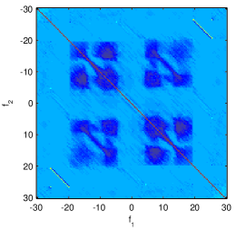
(c)

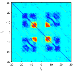
(d)

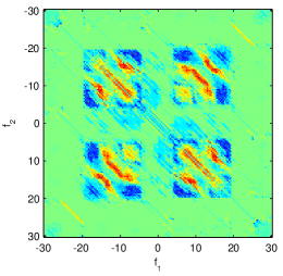
Figure 4: Plots (a) – (d): The first through fourth principal components of the thresholded cross-frequency coherence matrix.

Description of the Data. The EEG data in this paper is recorded from a healthy male college student from whom we recorded potentials from the scalp using a 64-channel EEG system (EMS, Biomed, Korneuburg, Germany). The electrodes were applied to the scalp using conventional methods arrayed in the standard International 10-20 system with two electrodes that served as a ground and a reference. The EEG was recorded at 512 Hertz and then band-pass filtered at (0.5,100) Hertz. An additional notch filter at 60 Hertz was applied to remove the artifact caused by the electrical power lines.

The participant performed a visually-guided hand movement task where he viewed a video monitor, placed about 1 meter away, and responded to targets that jumped to the left or right from a central position. A target jump, occurring every 1.5 5 second, instructed the participant to displace the lever of a hand-held joystick from a central upright position to realign the visual representation of the joystick orientation with the displaced target, either to the right or left of center. He received instructions to start and to move quickly and accurately, and to return the joystick to the center position only when the target jumped back to the center of the video monitor. We analyzed EEG signals for 138 rightward movements from the center position. From the montage of 64 scalp electrodes, we selected the FC3 electrode, presumably placed over the prefrontal cortex, which is demonstrated to be implicated in premotor processing [29]. The prefrontal cortex, in coordination with the parietal cortex (which is responsible for visual sensation) and the occipital cortex (which plays a key role in visual-motor transformations) are all engaged processing and execution of this visually-guided hand motor task.

Results and Discussion. We produced an estimate of $\tau^{(r)}(f_{1},f_{2})$ for each trial $r$. For illustrative purposes, in Figure 3 (a) and (c), we computed $\widehat{\tau}^{(r)}(f_{1},f_{2})$ for trials $r=1$ and $r=8$. Of course not all non-zero Loève dual-frequency coherence is really statistically significant. For each trial, we thresholded the estimated Loève dual frequency spectra using the marginal distribution of Equation (23) combined with the False Discovery Rates (FDR) procedure with a set rate of $5\%$ [26]. To avoid Hermitian redundancy and dependence, the Loève dual-frequency coherence matrix was subsampled to half its size over the frequency interval of interest $[-30,30]$ Hz before this procedure was applied. Two examples of estimated Loève coherence, derived from the thresholded Loève spectra, are shown in Figure 3 (b) and (d). We see two structures that clearly emerge from the thresholded spectra: one is the presence of “thin” lines and the other is the presence of fat “blobs”. The thin lines can be explained by the structure of a normal cyclostationary model, the fatter structure requires more modulation, like in Example 2. The blobs are not an effect of the multi-taper method even if this method essentially smooths the power across frequency: if the smearing was only due to a resolution issue then the two types of Loève spectra would not appear in the data. A plausible explanation of the spread is the distribution of oscillations (or spread of power across some frequency band) and the temporal nonstationarities of the oscillations’ amplitudes within a single trial is discussed in Section II-C.

Before combining information across trials, we first computed the average dual-frequency coherence across all trials and plotted the average of the magnitudes in Figure 1, averaged over batches of 20 trials. One must be cautious when averaging the complex quantities as phase shifts may average real features to zero. There appears to be some homogeneity of the response across trials, and so the distribution of magnitude of the coherence averaged over multiple trials is stable and similar (e.g. Figure 1 subplots (a), (b) and (c)). However, these are population results. To see trial-specific characteristics, we refer to individual estimates of the Loève coherence in Figure 3.

(a)

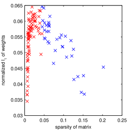
(b)

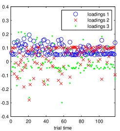
(c)

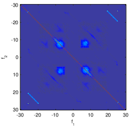
(d)

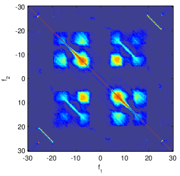
Figure 5: Plot (a): The sparsity of the matrix versus the sparsity across the loadings (recall the weights for each PC is normalized to one). Plot (b): The loads for the first three principal components versus trials. Plots (c) and (d): The mean of the two clusters of the weights.

A close examination of the individual estimates suggest that there are two subpopulations to this group of Loève (magnitude) coherence matrices. To further investigate this between-trials structure, we performed a singular value decomposition (or principal component analysis) on the magnitudes of the thresholded matrices in Figure 3. We plotted the first four principal components in Figure 4. The first principal component (PC) is very similar to the averages shown in Figure 1 (a) and thus the first PC represents a kind of “average”. The second PC in Figure 4(b) can either add to or subtract from the “squares” of Figure 1(a). The third and fourth PC in Figure 4(c) and (d) add additional structure.

(a)

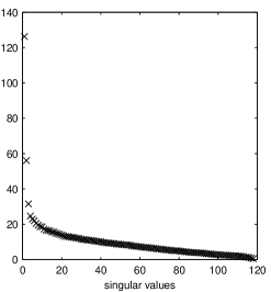
(b)

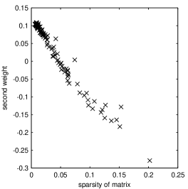
(c)

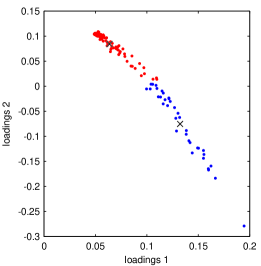
(d)

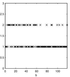
Figure 6: Plot (a): Singular values. Plot (b): The fraction of non-zero values of a matrix versus its weight to the second principal component. Plot (c): The first and second weights with colors superimposed to signify the clustering from the k-mean method. Plot (d): The labelling of each state across trials (d).

We plot the singular values in Figure 6(a). As already noted, the inclusion of the second principal component leads to substantially sparser correlations and the sparsity of the matrices is clearly correlated with the second weight (Figure 6(b)). We then used the k-means method to cluster the trials using only the first two sets of weights. This decision was made empirically by looking at the weights vs series (e.g. Figure 7(a) and (b)). The analysis yielded clearly made up groups, see Figure 6(c) where the sign of the second loadings decided the group to which the matrix belongs on trial $b$. There was a clear trial specific effect and we show the labels of groups versus trials in Figure 6(d), where for example cluster two becomes less frequent across trials.

The raw loadings utilized for clustering are displayed in Figure 5(b). Clearly the longer the subject waited, the higher the likelihood of diffuse correlation between frequencies, as shown in Figure 5(c) and (d). The effect of sparsity on the labels was also clear from Figure 5(a). Red color in the plots corresponds to the matrix in Figure 5(c), which was the sparser matrix in each trial, but this type of magnitude matrix was less sparse across components for some degrees of sparsity (see Figure 5(a)). It was less sparse across components because it was not as “empty” as seen from Figure 5(c), but corresponded to the structure with some extremely narrow lines as shown in Figure 3(b). This will require several principal components, each of which will be specific to each frequency that the brain can produce within a band. The more diffuse structures in Figure 3(d) is the blue color in the plots and is the fatter matrix in Figure 5(d). These oscillations were more variable within a trial, as discussed due to variable amplitudes within the trial, causing the narrow lines to spread.

In summary, our proposed modulated cyclostationary model captured highly significant and interesting interactions between the alpha ($8-12$ Hertz) and beta ($12-30$ Hertz) bands, as clear from Figure 5(d). These results would not have been obtained from the usual spectral analysis procedures – which ignore these types of interactions. Neither does the sparser structure of Figure 5(c) agree with a stationary model as negative and positive frequencies are correlated. This correlation corresponds to a synchrony of oscillations corresponding to starting at a given time after stimulus.

Our findings are interesting because they support the general consensus that the alpha and beta oscillations play significant individual roles during movement. [30] demonstrate that beta activity is closely linked to motor behavior and is generally attenuated during active movements. Moreover, studies have shown beta band activity to be significant even during just motor imagery and also for task switching. Alpha activity was indicated in [31] to reflect neural activity related to stages of motor response during a continuous monitoring task. In fact, in a similar response in beta power, alpha power is reduced at several central electrodes during response execution. Further studies demonstrated widespread high alpha ($10-12$ Hertz) coherence increase around the primary sensorimotor cortex during response execution, inhibition and preparation. While these studies show the contribution of the individual alpha and beta activity during movement, our findings suggest the association and some temporal alignment between these two oscillations which we submit to the neuroscience community for further interrogation.

(a)

(b)

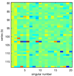
Figure 7: Plot (a): The weights across series and singular vectors for the first 20 trials. Plot (b): The weights across series and singular vectors for the last 20 trials.

V Discussion

Stationarity is a traditional assumption that enables consistent estimation of the covariance of a time series without replicated measurements. For this reason much of classical estimation theory relies on this assumption. As demonstrated in this paper, there are scenarios when this assumption is unreasonable. However, it is unclear what should be done if the assumption is relaxed, especially if there is no sense of replication between sets of observation.

In the absence of replication, a simpler model must be posited so that ${\cal O}(T^{2})$ covariances need not be estimated. If we insist on retaining a non-parametric model of covariances, then these must be changing slowly, to enable estimation. In contrast, with replication, a higher resolution estimate is feasible. To enable estimation with replication, a model for the form of replication must be constructed. As we have investigated in this paper, allowing for any randomness in phase can create destructive interference once combining information across replicates. We therefore propose to remove the phase of the Loève coherence to avoid this destructive interference.

Finally a sensible approach to extracting common features from the replicates must be designed: we here chose to formulate a model, which prompted us to use the singular value decomposition. If the entire time series data contains more than one population, straight averaging is not going to work even if the phase is removed. With straight averaging, the averages between the two populations will be recovered instead of a good estimate of each individual population. We show for simulated and real-life data how the singular value decomposition can recover the true underlying populations, and help us classify the state according to their frequency correlation. Smooth and visually appealing frequency correlation maps are produced from such (see Figures 5(c) and (d)).

There is an underlying philosophical issue from our analysis. Much effort has focused on defining time series models that are either stationary, or locally stationary in a traditional sense. However real-life data challenge the perception that such is pervasive and the silver bullet for time series applications. Traditional nonstationary models, such as the locally stationary model of Priestley [32] and [6], the SLEX (local Fourier) model in [33], and the locally stationary wavelet model in [34] are an extremely useful addition to the literature, but cannot capture all features of real data, such as correlation of strongly separated frequencies. Our addition of the modulated cyclostationary process is to introduce a new model class capable of capturing frequency correlation, but more flexible and parametric model classes are sorely needed. Until such are developed, non-parametric approaches are pivotal to learning additional characteristics of the data. Until such are developed so that we may estimate important features in single trials, we will need to use repeated trials to highlight and extract important time series characteristics. It is important to always investigate such possibilities when analyzing data, or important aspects of the data will be missed. This will cause us to not infer the correct generating mechanism of the data, and is so very serious.

Statistical Properties of the Fourier Transform

An arbitrary random vector $\mathbf{Z}$ which is complex-Gaussian is denoted as $\mathbf{Z}\overset{d}{=}N_{C}(\bm{\mu},\bm{\Sigma},\bm{C})$, which means the real and imaginary part are jointly Gaussian and

$$\mathrm{E}\{\mathbf{Z}\} = \bm{\mu}_{Z},\quad\mathrm{var}\{\mathbf{Z}\}=\mathrm{E}\{(\mathbf{Z}-\bm{\mu}_{Z})(\mathbf{Z}-\bm{\mu}_{Z})^{H}\}=\bm{\Sigma}_{Z}$$ (25)

$$\mbox{Rel}\{\mathbf{Z}\} = \mathrm{E}\{(\mathbf{Z}-\bm{\mu}_{Z})(\mathbf{Z}-\bm{\mu}_{Z})^{T}\}=\mathbf{C}_{Z}.$$ (26)

In the special case of $\mathbf{C}_{Z}=\mathbf{0}$ the distribution is complex-Gaussian proper and is written $\mathbf{Z}\overset{d}{=}N_{C,P}(\bm{\mu}_{Z},\bm{\Sigma}_{Z})$. For $\overline{I}^{(r)}_{\cdot}(f_{1},f_{2})$, we denote

$$\bm{\Sigma}_{Z}=S^{(r)}(f_{1},f_{2})\ \ {\mbox{and}}\ \ \mathbf{C}_{Z}=C^{(r)}(f_{1},f_{2})$$

By Isserlis’ theorem [35],

$$\mathrm{E}\left\{x_{k}^{(r)}(f_{1})x_{k}^{(r)\ast}(f_{2})\right\} = S^{(r)}(f_{1},f_{2}),\quad\mathrm{E}\left\{x_{k}^{(r)}(f_{1})x_{k}^{(r)}(f_{2})\right\}=C^{(r)}(f_{1},f_{2})$$

$$\mathrm{var}\left\{x_{k}^{(r)}(f_{1})x_{k}^{(r)\ast}(f_{2})\right\} = S^{(r)}(f_{1},f_{1})S^{(r)}(f_{2},f_{2})+\left|C^{(r)}(f_{1},f_{2})\right|^{2}$$

$$\mbox{Rel}\left\{x_{k}^{(r)}(f_{1})x_{k}^{(r)\ast}(f_{2})\right\} = C^{(r)}(f_{1},f_{1})C^{(r)\ast}(f_{2},f_{2})+\left(S^{(r)}(f_{1},f_{2})\right)^{2}.$$

For our convenience we define the variance and relation of $\overline{I}^{(r)}_{\cdot}(f_{1},f_{2})$ to be, respectively,

$$\sigma^{2}_{I}(f_{1},f_{2}) = \frac{S^{(r)}(f_{1},f_{1})S^{(r)}(f_{2},f_{2})+\left|R^{(r)}(f_{1},f_{2})\right|^{2}}{K}\in{\mathbb{R}}^{+},$$

$$c_{I}(f_{1},f_{2}) = \frac{R^{(r)}(f_{1},f_{1})R^{(r)\ast}(f_{2},f_{2})+\left(S^{(r)}(f_{1},f_{2})\right)^{2}}{K}\in{\mathbb{C}}.$$

Thus, for an arbitrary harmonizable process,

$$\overline{I}^{(r)}_{\cdot}(f_{1},f_{2}) = {\cal I}^{(r)}_{\cdot}(f_{1},f_{2})e^{-i\varphi^{(r)}_{\cdot}(f_{1},f_{2})}\quad\overset{d}{=}N_{C}\left(S^{(r)}(f_{1},f_{2}),\sigma^{2}_{I}(f_{1},f_{2}),c_{I}(f_{1},f_{2})\right)$$

where ${\cal I}^{(r)}_{\cdot}(f_{1},f_{2})\in{\mathbb{R}}^{+}$. If the process $X_{t}^{(r)}$ is stationary then $S^{(r)}(f_{1},f_{2})=S^{(r)}(f_{1})\delta(f_{1}-f_{2})$ and thus,

$$\overline{I}^{(r)}_{\cdot}(f_{1},f_{2})\overset{d}{\approx}N_{C}\left(S^{(r)}(f_{1})\delta(f_{1}-f_{2}),\frac{S^{(r)}(f_{1})S^{(r)}(f_{2})}{K},\frac{\left(S^{(r)}(f_{1})\right)^{2}\delta(f_{1}-f_{2})}{K}\right).$$ (27)

References

- [1] I. K. Kim and Y. Y. Kim, “Damage size estimation by the continuous wavelet ridge analysis of dispersive bending waves in a beam,” J. Sound Vib., vol. 287, pp. 707–722, 2005.
- [2] Z. P. Zhang, Z. Ren, and W. Y. Huang, “A novel detection method of motor broken rotor bars based on wavelet ridge,” IEEE Trans. Energy Conver., vol. 18, pp. 417–423, 2003.
- [3] S. C. Olhede and J. M. Lilly, “Analysis of modulated multivariate oscillations,” IEEE Transactions on Signal Processing, vol. 60, pp. 600–612, 2012.
- [4] S. D. Cranstoun, H. C. Ombao, R. von Sachs, W. S. Guo, and B. Litt, “Time-frequency spectral estimation of multichannel EEG using the auto-SLEX method,” IEEE Trans. on Biomedical Engineering, vol. 49, pp. 988–996, 2002.
- [5] H. Ombao, J. Raz, R. von Sachs, and B. Mallow, “Automatic statistical analysis of bivariate nonstationary time series,” J. Am. Stat. Assoc., vol. 96, pp. 543–560, 2001.
- [6] R. Dahlhaus, “A likelihood approximation for locally stationary processes,” The Annals of Statistics, vol. 28, pp. 1762–1794, 2000.
- [7] R. A. Silverman, “Locally stationary random processes,” IRE Trans. Information Theory, vol. 3, pp. 182–187, 1957.
- [8] E. G. Gladyshev, “Periodically correlated random sequences,” Soviet Math, vol. 2, pp. 385–388, 1961.
- [9] W. A. Gardner, A. Napolitano, and L. Paura, “Cyclostationarity: half a century of research,” Signal Processing, vol. 86, pp. 639–697, 2006.
- [10] W. A. Gardner, Cyclostationarity in Communications and Signal Processing. Piscataway: IEEE, 1994.
- [11] H. B. Voelcker, “Toward a unified theory of modulation. I. Phase-envelope relationships.” IEEE Transactions on Signal Processing, vol. 54, pp. 340–353, 1966.
- [12] H. Hindberg and A. Hanssen, “Generalized spectral coherences for complex-valued harmonizable processes,” IEEE Transactions on Signal Processing, vol. 55, pp. 2407–2413, 2007.
- [13] S. Sanei and J. A. Chambers, EEG Signal Processing. Cambridge, UK: CUP, 2007.
- [14] M. Loève, Probability theory. New York, USA: Van Nostrand, 1963.
- [15] K.-S. Lii and M. Rosenblatt, “Line spectral analysis for harmonizable processes,” Proceedings of the National Academy of Sciences of the United States of America, vol. 95, pp. 4800–4803, 1998.
- [16] ——, “Spectral analysis for harmonizable processes,” The Annals of Statistics, vol. 30, pp. 258–297, 2002.
- [17] E. G. Gladyshev, “Periodically and almost periodically correlated random sequences,” Theory Probab. Appl., vol. 8, pp. 137–177, 1963.
- [18] M. B. Priestley, Non-linear and Non-stationary time series. New York: Academic Press, 1988.
- [19] L. Cohen, Time-frequency analysis: Theory and applications. Upper Saddle River, NJ, USA: Prentice-Hall, Inc., 1995.
- [20] D. Thomson, “Spectrum estimation and harmonic analysis,” Proceedings of IEEE, vol. 70, pp. 1055–1096, 1982.
- [21] D. B. Percival and A. T. Walden, Spectral Analysis for Physical Applications. Cambridge, UK: Cambridge University Press, 1993.
- [22] R. J. Mellors, F. L. Vernon, and D. J. Thomson, “Detection of dispersive signals using multitaper dual-frequency,” Geophysical Journal International, vol. 135, pp. 146–154, 1998.
- [23] S. Cambanis, C. Houdré, H. Hurd, and J. Leskow, “Laws of large numbers for periodically and almost periodically correlated processes,” Stochastic Processes and Their Application, vol. 53, pp. 37–54, 1994.
- [24] D. R. Brillinger, Time Series: Data Analysis and Theory. Philadelphia: SIAM, 2001.
- [25] P. J. Schreier and L. L. Scharf, Statistical Signal Processing of Complex-Valued Data. Cambridge, UK: Cambridge University Press, 2010.
- [26] B. Efron, Large-Scale Inference. Cambridge UK: Cambridge University Press, 2010.
- [27] G. Gan, C. Ma, and J. Wu, Data Clustering: Theory, Algorithms, and Applications. Philadelphia, USA: SIAM, 2007.
- [28] M. B. Priestley, Spectral analysis and Time Series. New York: Academic Press, 1981.
- [29] B. Marconi, A. Genovesio, A. Battaglia-Mayer, S. Ferraina, S. Squatrito, M. Molinari, F. Lacquaniti, and R. Caminiti, “Eye-hand coordination during reaching. I. anatomical relationships between parietal and frontal cortex,” Cerebral Cortex, vol. 11, pp. 513–527, 2001.
- [30] G. Pfurtscheller and F. L. da Silva, “Event-related eeg/meg syn- chronization and desynchronization: basic principles,” Clinical Neurophysiology, vol. 110, pp. 1842–1857, 1999.
- [31] R. Moore, A. Gale, P. Morris, and D. Forrester, “Alpha power and coherence primarily reflect neural activity related to stages of motor response during a continuous monitoring task,” International Journal of Psychophysiology, vol. 69, pp. 79–89, 2008.
- [32] M. B. Priestley, “Evolutionary spectra and non-stationary processes,” J. Roy. Stat. Soc., B, vol. 27, pp. 204–237, 1965.
- [33] H. Ombao, R. von Sachs, and W. Guo, “Slex analysis of multivariate non-stationary time series,” J. Am. Stat. Assoc., vol. 100, pp. 519–531, 2005.
- [34] G. P. Nason, R. von Sachs, and G. Kroisandt, “Wavelet processes and adaptive estimation of the evolutionary wavelet spectrum,” J. Roy. Stat. Soc., B, vol. 62, 2000.
- [35] L. Isserlis, “On a formula for the product-moment coefficient of any order of a normal frequency distribution in any number of variables,” Biometrika, vol. 12, pp. 134–139, 1918.