A stabilized Nitsche fictitious domain method for the Stokes problem

Abstract

We develop a Nitsche fictitious domain method for the Stokes problem starting from a stabilized Galerkin finite element method with low order elements for both the velocity and the pressure. By introducing additional penalty terms for the jumps in the normal velocity and pressure gradients in the vicinity of the boundary, we show that the method is inf-sup stable. As a consequence, optimal order a priori error estimates are established. Moreover, the condition number of the resulting stiffness matrix is shown to be bounded independently of the location of the boundary. We discuss a general, flexible and freely available implementation of the method in three spatial dimensions and present numerical examples supporting the theoretical results.

1 Introduction

A frequently encountered problem in practical applications of the finite element method is the generation of a high quality mesh conforming to the computational domain. For instance, the simulation of flow around an object embedded in a channel typically requires a mesh discretizing the domain surrounding the object. If the domain is complex, the mesh generation problem is highly non-trivial. Furthermore, the mesh must be modified or regenerated each time the object is translated, scaled or rotated, for example to study the lift or drag for different angles of attack.

In fictitious domain finite element methods [16, 17, 37, 22], the computational domain is instead represented by a, possibly regular, background mesh and an interior surface; this situation is illustrated in Figure 1.1. The mesh generation problem is thus essentially avoided. However, new challenges are introduced. The interior surface must be represented and the intersection of the surface and the underlying mesh computed, which is a complex task for three-dimensional domains. Moreover, the finite element formulation, and hence also its analysis and implementation, involves elements of non-regular shapes induced by this intersection.

Fig. 1.1: The stabilized Nitsche fictitious domain method presented in this work allows the simulation of Stokes flow around a possibly complex object (in this simplified illustration, a two-dimensional airfoil) embedded in a fixed background mesh. The object is defined by its boundary $\Gamma$, and the computational mesh (here the cut mesh surrounding the airfoil) is defined as the intersection of the fixed background mesh and the outside (or inside) of the boundary $\Gamma$.

In this work, we consider a Nitsche fictitious domain method for the Stokes problem: find the velocity $\boldsymbol{u}:\Omega\subset\mathbb{R}^{d}\rightarrow\mathbb{R}^{d}$ and the pressure $p:\Omega\to\mathbb{R}$ such that

$$-\Delta\boldsymbol{u}+\nabla p =\boldsymbol{f} \text{in $\Omega$},$$ (1.1a)

$$\nabla\cdot\boldsymbol{u} =0 \text{in $\Omega$},$$ (1.1b)

$$\boldsymbol{u} =\boldsymbol{g} \text{on $\Gamma$},$$ (1.1c)

where $\Omega$ denotes a bounded domain in $\mathbb{R}^{d}$, $d=2$ or $3$, with Lipschitz boundary $\Gamma$, and where $\boldsymbol{f}\in L^{2}(\Omega)$ is a given body force and $\boldsymbol{g}\in H^{1/2}(\Gamma)$ is a prescribed boundary velocity. To satisfy (1.1b), we assume that $\int_{\Gamma}\boldsymbol{n}\cdot\boldsymbol{g}\,\mathrm{d}s=0$ where $\boldsymbol{n}$ denotes the outward pointing boundary normal. Moreover, we assume that $\int_{\Omega}p\,\mathrm{d}x=0$ to uniquely determine $p$.

The fictitious domain method introduced in this paper is based on a least squares stabilized finite element method with low order finite element spaces. In particular, we consider both the case of continuous piecewise linear vector fields for the velocity and continuous piecewise linears for the pressure, and the case of continuous piecewise linear vector fields for the velocity and piecewise constants for the pressure. We prove stability and optimal a priori error estimates as well as optimal estimates for the condition number. These results rely on the introduction of stabilization terms for the jump in the normal gradients at faces associated with elements intersecting the boundary. Our method is closely related to a very recent report of Burman and Hansbo [12], but the analysis follows a different route. The present work also differs from that of Burman and Hansbo [12] in that our methodology has been tested and implemented in three dimensions. Similar results have been obtained for elliptic boundary problems by Burman [10], Burman and Hansbo [11] and Johansson and Larson [22]. In a related work [30], we present a stabilized Nitsche overlapping mesh method for the Stokes problem.

A central and unique contribution of the current work is the full and general treatment of domains represented by arbitrary boundary triangulations embedded in three-dimensional tetrahedral meshes. This requires integration over arbitrary polyhedral domains resulting from the subtraction of the embedded domain from the background mesh. The intersection of the boundary and the background mesh is computed efficiently using techniques from computational geometry. The freely available implementation is based on, but extends that of, our previous work [29].

The remainder of this paper is organized as follows. In Section 2, we summarize the notation and assumptions used throughout this work. The novel Nitsche fictitious domain finite element formulation for the Stokes problem is then introduced in Section 3, while Sections 4–6 are devoted to its a priori error analysis. We prove that the condition number is bounded independently of the location of the boundary in Section 7. A brief summary of key implementation aspects is provided in Section 8, along with numerical investigations corroborating the theoretical results and an example demonstrating the applicability of the developed framework to complex 3D geometries. Finally, we provide some concluding remarks in Section 9.

2 Preliminaries

The Nitsche fictitious domain finite element formulation involves integration over various geometric entities. We here define these entities and summarize the notation that will be used throughout this paper for computational domains, meshes, function spaces and norms.

2.1 Computational domain and meshes

Let $\Omega$ be an open, bounded domain in $\mathbb{R}^{d}$ ($d=2,3$) with Lipschitz boundary $\Gamma$. We assume that $\Omega$ is a subset of a larger polygonal domain $\Omega^{\ast}$; that is, $\Omega\subset\Omega^{\ast}$. We will refer to $\Omega^{\ast}$ as the fictitious domain. Let $\mathcal{T}^{\ast}$ be a shape-regular tessellation of $\Omega^{\ast}$ such that $T\cap\Omega\neq\emptyset$ for all $T\in\mathcal{T}^{\ast}$. The mesh $\mathcal{T}^{\ast}$ might be constructed from a larger and easy-to-generate mesh $\widehat{\mathcal{T}^{\ast}}$ by extracting a suitable submesh, cf. Figure 2.1. A facet $F$; that is, an edge in two dimensions or a face in three dimensions, of the mesh $\mathcal{T}^{\ast}$ is labeled an exterior facet if it belongs to one element only (and is thus a part of the boundary of $\Omega^{\ast}$) or an interior facet if it is shared by two elements. In the latter case, we denote the two elements shared by the facet $F$ by $T^{+}_{F}$ and $T^{-}_{F}$. The set of all exterior facets defines the boundary mesh $\partial_{e}\mathcal{T}^{\ast}$, while the set of all interior facets defines the skeleton mesh $\partial_{i}\mathcal{T}^{\ast}$.

Fig. 2.1: (Left) The computational domain $\Omega$ is defined as the inside or outside of a given boundary $\Gamma$ imposed on a fixed background mesh $\widehat{\mathcal{T}^{\ast}}$. (Right) The fictitious domain $\Omega^{\ast}$ is the union of the minimal subset $\mathcal{T}^{\ast}\subset\widehat{\mathcal{T}^{\ast}}$ covering $\Omega$.

Given $\mathcal{T}^{\ast}$, we may define the cut mesh $\mathcal{T}$ on $\Omega$ as follows:

$$\mathcal{T}=\{T\cap\overline{\Omega}:T\in\mathcal{T}^{\ast}\}.$$ (2.1)

The corresponding boundary and skeleton meshes are defined accordingly by $\partial_{e}\mathcal{T}=\{F\cap\overline{\Omega}:F\in\partial_{e}\mathcal{T}^{\ast}\}$ and $\partial_{i}\mathcal{T}=\{F\cap\overline{\Omega}:F\in\partial_{i}\mathcal{T}^{\ast}\}$. Note that $\mathcal{T}$, $\partial_{e}\mathcal{T}$ and $\partial_{i}\mathcal{T}$ consist of both standard (simplicial) elements and facets, and non-standard elements and facets. We will occasionally refer to the former set as non-cut elements or facets, and the latter set as cut elements or facets.

Next, let $\mathcal{T}^{\ast}_{\Gamma}$ be the subset of elements in $\mathcal{T}^{\ast}$ that intersect the boundary $\Gamma$:

$$\mathcal{T}^{\ast}_{\Gamma}=\{T\in\mathcal{T}^{\ast}:T\cap\Gamma\neq\emptyset\}$$ (2.2)

and introduce the notation $\mathcal{F}^{\ast}_{\Gamma}$ for the set of all interior facets belonging to elements intersected by the boundary $\Gamma$:

$$\mathcal{F}^{\ast}_{\Gamma}=\{F\in\partial_{i}\mathcal{T}^{\ast}:\;T^{+}_{F}\cap\Gamma\neq\emptyset\vee T^{-}_{F}\cap\Gamma\neq\emptyset\}.$$ (2.3)

Figure 2.2 illustrates this notation.

We assume that $\mathcal{T}^{\ast}$ and the boundary $\Gamma$ satisfy the following geometric conditions:

• G1: The intersection between $\Gamma$ and a facet $F\in\partial_{i}\mathcal{T}^{\ast}$ is simply connected; that is, $\Gamma$ does not cross an interior facet multiple times.

• G2: For each element $T$ intersected by $\Gamma$, there exists a plane $S_{T}$ and a piecewise smooth parametrization $\Phi:S_{T}\cap T\rightarrow\Gamma\cap T$.

• G3: We assume that there is an integer $N>0$ such that for each element $T\in\mathcal{T}^{\ast}_{\Gamma}$ there exists an element $T^{\prime}\in\mathcal{T}^{\ast}\setminus\mathcal{T}^{\ast}_{\Gamma}$ and at most $N$ elements $\{T\}_{i=1}^{N}$ such that $T_{1}=T,\,T_{N}=T^{\prime}$ and $T_{i}\cap T_{i+1}\in\partial_{i}\mathcal{T}^{\ast},\;i=1,\ldots N-1$. In other words, the number of facets to be crossed in order to “walk” from a cut element $T$ to a non-cut element $T^{\prime}\subset\Omega$ is bounded.

Similar assumptions were made by Hansbo and Hansbo [18], Burman and Hansbo [11] for the two dimensional case and ensure that $\Gamma$ is reasonably resolved by $\mathcal{T}^{\ast}$.

Fig. 2.2: The boundary zone of the fictitious domain. (Left) The background mesh $\mathcal{T}^{\ast}$ together with the cut mesh $\mathcal{T}$. Observe that for the element associated with the node $\boldsymbol{x}$, only a small fraction resides inside the domain $\Omega$. (Right) The elements in yellow are intersected by the boundary and therefore part of the mesh $\mathcal{T}^{\ast}_{\Gamma}$. Interior facets of elements intersected by the boundary ($\mathcal{F}^{\ast}_{\Gamma}$) are marked in green.

2.2 Finite element spaces

We let the discrete velocity space $V_{h}$ be the space of continuous, piecewise linear $\mathbb{R}^{d}$-valued vector fields defined relative to a specified mesh, and let the pressure space $Q_{h}$ consist of either piecewise constant or continuous piecewise linear elements, denoted by $P_{h}^{0,\mathrm{dc}}$ and $P_{h}^{1}$, respectively.

Here and below, let $\|\cdot\|_{s,\Omega}$ and $|\cdot|_{s,\Omega}$ denote the standard Sobolev norms and semi-norms on a domain $\Omega$ for $s\in\mathbb{N}$. The corresponding inner products are denoted by $(\cdot,\cdot)_{s,\Omega}$. For $s=0$, the subscript $s$ is omitted. Furthermore, we introduce the following mesh-dependent norms for the velocity:

$$|\mspace{-1.0mu}|\mspace{-1.0mu}|\boldsymbol{v}|\mspace{-1.0mu}|\mspace{-1.0mu}|^{2} =\|\nabla\boldsymbol{v}\|^{2}_{\Omega}+\|h^{-1/2}\boldsymbol{v}\|^{2}_{\Gamma}+\|h^{1/2}\boldsymbol{n}\cdot\nabla\boldsymbol{v}\|^{2}_{\Gamma},$$ (2.4)

$$|\mspace{-1.0mu}|\mspace{-1.0mu}|\boldsymbol{v}|\mspace{-1.0mu}|\mspace{-1.0mu}|_{\ast}^{2} =\|\nabla\boldsymbol{v}\|^{2}_{\Omega^{\ast}}+\|h^{-1/2}\boldsymbol{v}\|^{2}_{\Gamma},$$ (2.5)

for the pressure:

$$|\mspace{-1.0mu}|\mspace{-1.0mu}|q|\mspace{-1.0mu}|\mspace{-1.0mu}|^{2} =\|q\|^{2}_{\Omega}+\|h^{1/2}q\|^{2}_{\Gamma},$$ (2.6)

$$|\mspace{-1.0mu}|\mspace{-1.0mu}|q|\mspace{-1.0mu}|\mspace{-1.0mu}|^{2}_{\ast} =\|q\|_{\Omega^{\ast}}^{2},$$ (2.7)

and for the product space:

$$|\mspace{-1.0mu}|\mspace{-1.0mu}|(\boldsymbol{v},q)|\mspace{-1.0mu}|\mspace{-1.0mu}|^{2} =|\mspace{-1.0mu}|\mspace{-1.0mu}|\boldsymbol{v}|\mspace{-1.0mu}|\mspace{-1.0mu}|^{2}+|\mspace{-1.0mu}|\mspace{-1.0mu}|q|\mspace{-1.0mu}|\mspace{-1.0mu}|^{2},$$ (2.8)

$$|\mspace{-1.0mu}|\mspace{-1.0mu}|(\boldsymbol{v},q)|\mspace{-1.0mu}|\mspace{-1.0mu}|^{2}_{\ast} =|\mspace{-1.0mu}|\mspace{-1.0mu}|\boldsymbol{v}|\mspace{-1.0mu}|\mspace{-1.0mu}|^{2}_{\ast}+|\mspace{-1.0mu}|\mspace{-1.0mu}|q|\mspace{-1.0mu}|\mspace{-1.0mu}|_{\ast}^{2}.$$ (2.9)

Note that the $|\mspace{-1.0mu}|\mspace{-1.0mu}|\cdot|\mspace{-1.0mu}|\mspace{-1.0mu}|_{\ast}$-norms are defined on the fictitious domain $\Omega^{\ast}$ and therefore represent proper norms for the discrete finite element functions. When mesh-dependent norms are applied to non-finite element functions on a domain $\Omega$, we always mean the evaluation of the norm on a tessellation $\mathcal{T}$ of $\Omega$.

3 Finite element formulation

Before we present the Nitsche fictitious domain method, we review a pair of well-established stabilized finite element formulations for the Stokes problem. These formulations are then extended to a Nitsche-based fictitious domain method.

3.1 Stabilized Stokes elements

Let $V_{h}$ and $Q_{h}$ be the velocity and pressure spaces introduced in the previous section defined relative to a standard conforming tessellation $\mathcal{T}$ of $\Omega$ and recall that $Q_{h}$ is defined to be either $P_{h}^{1}$ or $P_{h}^{0,\mathrm{dc}}$. It is well-known that the mixed spaces $V_{h}\times P_{h}^{1}$ and $V_{h}\times P_{h}^{0,\mathrm{dc}}$ violate the inf-sup condition for the ${[H^{1}_{0}(\Omega)]^{d}}\times L^{2}(\Omega)/\mathbb{R}$ variational formulation of the Stokes problem (1.1), and thus, are not stable in the Babuška–Brezzi sense [9]. Different strategies can be employed to compensate for the lack of stability [19, 20, 23, 7], whereof consistently stabilized methods are among the most prominent [14, 5]. Here, we consider consistently stabilized discrete variational formulations of (1.1), with $\boldsymbol{g}=0$, of the following form: find $(\boldsymbol{u}_{h},p_{h})\in V_{h}\times Q_{h}$ such that

$$A_{h}(\boldsymbol{u}_{h},p_{h};\boldsymbol{v}_{h},q_{h})=L_{h}(\boldsymbol{v}_{h},q_{h})\quad\forall\,(\boldsymbol{v}_{h},q_{h})\in V_{h}\times Q_{h},$$ (3.1)

where the bilinear and linear forms $A_{h}$ and $L_{h}$ are defined by

$$A_{h}(\boldsymbol{u}_{h},p_{h};\boldsymbol{v}_{h},q_{h}) =a_{h}(\boldsymbol{u}_{h},\boldsymbol{v}_{h})+b_{h}(\boldsymbol{u}_{h},q_{h})+b_{h}(\boldsymbol{v}_{h},p_{h})-c_{h}(\boldsymbol{u}_{h},p_{h};q_{h}),$$

$$L_{h}(\boldsymbol{v}_{h},q_{h}) =(\boldsymbol{f},\boldsymbol{v}_{h})-\Phi_{h}(q_{h}).$$ (3.2)

Here, $a_{h}$ and $b_{h}$ are the standard forms

$$a_{h}(\boldsymbol{u}_{h},\boldsymbol{v}_{h}) =(\nabla\boldsymbol{u}_{h},\nabla\boldsymbol{v}_{h})_{\Omega},$$ (3.3)

$$b_{h}(\boldsymbol{v}_{h},p_{h}) =-(\nabla\cdot\boldsymbol{v}_{h},p_{h})_{\Omega}.$$ (3.4)

The stabilization form $c_{h}$ is given by

$$c_{h}(\boldsymbol{u}_{h},p_{h};q_{h}) =\begin{cases}\beta_{0}\sum_{F\in\partial_{i}\mathcal{T}}\,h_{F}([p_{h}],[q_{h}])_{F}&\quad\text{if }Q_{h}=P_{h}^{0,\mathrm{dc}},\\ \beta_{1}\sum_{T\in\mathcal{T}}\,h_{T}^{2}(-\Delta\boldsymbol{u}_{h}+\nabla p_{h},\nabla q_{h})_{T}&\quad\text{if }Q_{h}=P_{h}^{1},\\ \end{cases}$$ (3.5)

where $h_{T}$ denotes the diameter of element $T$, $h_{F}$ denotes the average of the diameters of the elements sharing a facet $F$, $[v]=v^{+}-v^{-}$ is the jump in a function $v$ over each facet $F$: $v^{\pm}(\boldsymbol{x})=\lim_{t\rightarrow 0^{+}}v(\boldsymbol{x}\pm t\boldsymbol{n})$ for $\boldsymbol{x}\in F$, and $\beta_{0}$ and $\beta_{1}$ are positive stabilization constants. In the case $Q_{h}=P_{h}^{1}$, this stabilization is also known as the pressure-Poisson stabilized Galerkin method. Note that $-\Delta\boldsymbol{u}_{h}$ vanishes if $\boldsymbol{u}_{h}$ is piecewise linear and is only included to clarify that the method is indeed consistent. We will therefore simply write $c_{h}(p_{h},q_{h})$ when only finite element functions are involved. The form $\Phi_{h}$ in (3.2) is, to ensure consistency, defined to be

$$\Phi_{h}(q_{h}) =\begin{cases}0&\quad\text{\hskip 3.0pt if }Q_{h}=P_{h}^{0,\mathrm{dc}},\\ \beta_{1}\sum_{T\in\mathcal{T}}h_{T}^{2}(\boldsymbol{f},\nabla q_{h})_{T}&\quad\text{\hskip 3.0pt if }Q_{h}=P_{h}^{1}.\end{cases}$$ (3.6)

Since $[q_{h}]=0$ for $q_{h}\in P_{h}^{1}$ and $\nabla(q_{h}|_{T})=0$ for $q_{h}\in P_{h}^{0,\mathrm{dc}}$, we may express the two cases in a more compact notation:

$$c_{h}(p_{h},q_{h}) ={\beta_{0}\sum_{F\in\partial_{i}\mathcal{T}}h_{F}([p_{h}],[q_{h}])_{F}}+{\beta_{1}\sum_{T\in\mathcal{T}}h_{T}^{2}(\nabla p_{h},\nabla q_{h})_{T}},$$ (3.7)

$$\Phi_{h}(q_{h}) =\beta_{1}\sum_{T\in\mathcal{T}}h_{T}^{2}(\boldsymbol{f},\nabla q_{h})_{T}.$$ (3.8)

3.2 A stabilized Nitsche fictitious domain method

Prior to stating the stabilized Nitsche fictitious domain formulation for the Stokes problem, we introduce the following forms with reference to the notation established in Section 2.1:

$$a_{h}(\boldsymbol{u}_{h},\boldsymbol{v}_{h}) =(\nabla\boldsymbol{u}_{h},\nabla\boldsymbol{v}_{h})_{\Omega}-(\partial_{\boldsymbol{n}}\boldsymbol{u}_{h},\boldsymbol{v}_{h})_{\Gamma}-(\partial_{\boldsymbol{n}}\boldsymbol{v}_{h},\boldsymbol{u}_{h})_{\Gamma}+\gamma(h^{-1}\boldsymbol{u}_{h},\boldsymbol{v}_{h})_{\Gamma},$$ (3.9)

$$b_{h}(\boldsymbol{v}_{h},p_{h}) =-(\nabla\cdot\boldsymbol{v}_{h},p_{h})_{\Omega}+(\boldsymbol{n}\cdot\boldsymbol{v}_{h},p_{h})_{\Gamma},$$ (3.10)

where $\partial_{\boldsymbol{n}}\boldsymbol{v}=\boldsymbol{n}\cdot\nabla\boldsymbol{v}$. Next, we introduce the velocity “ghost-penalty” form:

$$i_{h}(\boldsymbol{u}_{h},\boldsymbol{v}_{h}) =\beta_{2}\sum_{F\in\mathcal{F}^{\ast}_{\Gamma}}h_{F}([\partial_{\boldsymbol{n}}\boldsymbol{u}_{h}],[\partial_{\boldsymbol{n}}\boldsymbol{v}_{h}])_{F},$$ (3.11)

and the pressure “ghost-penalty” form:

$$j_{h}(p_{h},q_{h}) =\begin{cases}\beta_{0}\sum_{F\in{\mathcal{F}^{\ast}_{\Gamma}}}h_{F}([p_{h}],[q_{h}])_{F\setminus\Omega}&\quad\text{if }Q_{h}=P_{h}^{0,\mathrm{dc}},\\ \beta_{3}\sum_{F\in\mathcal{F}^{\ast}_{\Gamma}}h_{F}^{3}([\partial_{\boldsymbol{n}}p_{h}],[\partial_{\boldsymbol{n}}q_{h}])_{F}&\quad\text{if }Q_{h}=P_{h}^{1}.\end{cases}$$ (3.12)

Again, $[v]=v^{+}-v^{-}$ is the jump over each facet $F$, and $\boldsymbol{n}=\boldsymbol{n}_{F}$ is a fixed, but arbitrary, unit normal to the facet $F$. Here, $\beta_{2}>0$ and $\beta_{3}>0$ denote additional penalty parameters. As before, we are allowed to rewrite (3.12) as a single form $j_{h}(p_{h},q_{h})=j_{h,0}(p_{h},q_{h})+j_{h,1}(p_{h},q_{h})$ with $j_{0,h}$ and $j_{h,1}$ denoting (3.12) in the case of $Q_{h}=P_{h}^{0,\mathrm{dc}}$ and $Q_{h}=P_{h}^{1}$, respectively.

We are now ready to state the Nitsche based fictitious domain method for the Stokes problem (1.1). Let $V_{h}=V_{h}(\mathcal{T}^{\ast})$ and $Q_{h}=Q_{h}(\mathcal{T}^{\ast})$ be the finite element velocity and pressure spaces defined relative to $\mathcal{T}^{\ast}$. The variational problem reads: find $(\boldsymbol{u}_{h},p_{h})\in V_{h}\times Q_{h}$ such that

$$A_{h}(\boldsymbol{u}_{h},p_{h};\boldsymbol{v}_{h},q_{h})+J_{h}(\boldsymbol{u}_{h},p_{h};\boldsymbol{v}_{h},q_{h})=L_{h}(\boldsymbol{v}_{h},q_{h})\quad\forall\,(\boldsymbol{v}_{h},q_{h})\in V_{h}\times Q_{h},$$ (3.13)

where $A_{h}$ and $J_{h}$ are defined by

$$A_{h}(\boldsymbol{u}_{h},p_{h};\boldsymbol{v}_{h},q_{h}) =a_{h}(\boldsymbol{u}_{h},\boldsymbol{v}_{h})+b_{h}(\boldsymbol{u}_{h},q_{h})+b_{h}(\boldsymbol{v}_{h},p_{h})-c_{h}(p_{h},q_{h}),$$ (3.14)

$$J_{h}(\boldsymbol{u}_{h},p_{h};\boldsymbol{v}_{h},q_{h}) =i_{h}(\boldsymbol{u}_{h},\boldsymbol{v}_{h})-j_{h}(p_{h},q_{h}),$$ (3.15)

where the forms $c_{h}$ and $\Phi_{h}$ are defined as in (3.7) and (3.8) (relative to the cut mesh $\mathcal{T}$). The form $L_{h}$ is given by

$$L_{h}(\boldsymbol{v}_{h},q_{h})=(\boldsymbol{f},\boldsymbol{v}_{h})_{\Omega}+(\boldsymbol{g},\gamma h^{-1}\boldsymbol{v}_{h}-\partial_{\boldsymbol{n}}\boldsymbol{v}_{h}+q_{h}\boldsymbol{n})_{\Gamma}-\Phi_{h}(q_{h}).$$ (3.16)

Remark 3.1.

The “ghost-penalty” defined in (3.11) was introduced by Burman and Hansbo [11] to formulate a first-order convergent fictitious domain method for the Poisson problem. The role of the ghost-penalty is to augment the bilinear form $a_{h}$ by accounting for small elements $|T\cap\Omega|\ll|T|,\;T\in\mathcal{T}^{\ast}$ in the vicinity of the boundary $\Gamma$.

Remark 3.2.

In the Stokes problem, the stabilization form $c_{h}$ acting on the pressure also has to be augmented. Depending on the pressure discretization, this can be achieved in different ways. In the case of $Q_{h}=P_{h}^{0,\mathrm{dc}}$, a similar ghost-penalty was presented by Becker et al. [6] to propose a finite element method for incompressible elasticity problems with discontinuous modulus of elasticity. To motivate the ghost-penalty (3.12) when $Q_{h}=P_{h}^{1}$, one may consider the stabilization terms $h_{T}^{2}(\nabla p,\nabla q)_{T}$ and $h_{T}^{2}(\boldsymbol{f},\nabla q)_{T}$ as a locally scaled version of a Poisson equation and apply (3.11). In Lemma 5.1, we will reveal the basic structure behind the augmentation terms and also present a generalization to higher-order elements.

4 Approximation properties

Before we proceed with the a priori error analysis of the method proposed in Section 3.2, we summarize here some notation and useful inequalities that will be used throughout Sections 5 and 6. In what follows, $\mathcal{V}_{h}^{\ast}$ and $\mathcal{V}_{h}$ denote some finite element spaces consisting of piecewise polynomial functions defined on $\mathcal{T}^{\ast}$ and $\mathcal{T}$ respectively, but it should be clear that we have mainly $\mathcal{V}_{h}=V_{h}$ or $\mathcal{V}_{h}=Q_{h}$ in mind. The constants $C$ involved in the inequalities will only depend on $\Omega$ or $\Omega^{\ast}$, the regularity of the relevant function spaces, the shape-regularity of $\mathcal{T}^{\ast}$, and possibly the polynomial order of $\mathcal{V}_{h}$; in particular, the constants $C$ do not depend on $h$.

4.1 Trace inequalities and inverse estimates

We recall the following trace inequalities for $v\in H^{1}(\Omega^{\ast})$:

$$\|v\|_{\partial T} \leqslant C(h_{T}^{-1/2}\|v\|_{T}+h_{T}^{1/2}\|\nabla v\|_{T})\quad\forall\,T\in\mathcal{T}^{\ast},$$ (4.1)

$$\|v\|_{T\cap\Gamma} \leqslant C(h_{T}^{-1/2}\|v\|_{T}+h_{T}^{1/2}\|\nabla v\|_{T})\quad\forall\,T\in\mathcal{T}^{\ast}.$$ (4.2)

See Hansbo and Hansbo [18] for a proof of (4.2). We will also need the following well-known inverse estimates for $v_{h}\in\mathcal{V}_{h}$:

$$\|\nabla v_{h}\|_{T} \leqslant Ch_{T}^{-1}\|v_{h}\|_{T} \forall\,T\in\mathcal{T}^{\ast},$$ (4.3)

$$\|h^{1/2}\boldsymbol{n}\cdot\nabla v_{h}\|_{F} \leqslant C\|\nabla v_{h}\|_{T} \forall\,T\in\mathcal{T}^{\ast},$$ (4.4)

For proofs, we refer to Quarteroni [31]. Moreover, we will need a version of (4.4) for the boundary parts $\Gamma\cap T$:

$$\|h^{1/2}\boldsymbol{n}\cdot\nabla v_{h}\|_{\Gamma\cap T}\leqslant C\|\nabla v_{h}\|_{T}\quad\forall\,T\in\mathcal{T}^{\ast},$$ (4.5)

which was proved under assumptions similar to G1 – G2 by Hansbo and Hansbo [18]. We note that for $\boldsymbol{v}_{h}\in V_{h}$, $q_{h}\in Q_{h}$, we have the two estimates:

$$|\mspace{-1.0mu}|\mspace{-1.0mu}|\boldsymbol{v}_{h}|\mspace{-1.0mu}|\mspace{-1.0mu}|\leqslant C|\mspace{-1.0mu}|\mspace{-1.0mu}|\boldsymbol{v}_{h}|\mspace{-1.0mu}|\mspace{-1.0mu}|_{\ast},\qquad|\mspace{-1.0mu}|\mspace{-1.0mu}|q_{h}|\mspace{-1.0mu}|\mspace{-1.0mu}|\leqslant C|\mspace{-1.0mu}|\mspace{-1.0mu}|q_{h}|\mspace{-1.0mu}|\mspace{-1.0mu}|_{\ast},$$ (4.6)

which can easily be deduced by (4.5), and by combining (4.2) and (4.3).

4.2 Interpolation estimates

In order to construct an interpolation operator $L^{2}(\Omega)\rightarrow\mathcal{V}_{h}$, we recall that there is a linear extension operator $\mathcal{E}:H^{s}(\Omega)\rightarrow H^{s}(\Omega^{\ast})$, $s\geqslant 0$, such that

$$\|\mathcal{E}u\|_{s,\Omega^{\ast}}\leqslant C\|u\|_{s,\Omega}.$$ (4.7)

See Stein [33] for further details. Let $\pi^{\ast}_{h}:L^{2}(\Omega^{\ast})\rightarrow\mathcal{V}^{\ast}_{h}$ be the standard Scott–Zhang interpolation operator [32] and recall the interpolation error estimates

$$\|v-\pi^{\ast}_{h}v\|_{r,T} \leqslant Ch^{s-r}|v|_{s,\omega(T)}, \quad 0\leqslant r\leqslant s\leqslant 2\quad \forall\,T\in\mathcal{T}^{\ast},$$ (4.8)

$$\|v-\pi^{\ast}_{h}v\|_{r,F} \leqslant Ch^{s-r-1/2}|v|_{s,\omega(T)}, \quad 0\leqslant r\leqslant s\leqslant 2\quad \forall\,F\in\partial_{i}\mathcal{T}^{\ast},$$ (4.9)

where $\omega(T)$ is the patch of neighbors of element $T$; that is, the domain consisting of all elements sharing a vertex with $T$. Next, we define $\pi_{h}:L^{2}(\Omega)\rightarrow\mathcal{V}^{\ast}_{h}$ as follows:

$$\pi_{h}v=\pi^{\ast}_{h}\mathcal{E}v.$$ (4.10)

Note that $\pi_{h}v$ is now defined on $\Omega^{\ast}$, and in particular on $\Omega\subset\Omega^{\ast}$.

The stability estimate (4.7) together with the interpolation error estimates (4.8) and (4.9) for the Scott–Zhang interpolation operator imply the following interpolation estimates:

$$\|v-\pi_{h}v\|_{r,T} \leqslant Ch^{s-r}|v|_{s,\omega(T)}, \quad 0\leqslant r\leqslant s\leqslant 2\quad \forall\,T\in\mathcal{T},$$ (4.11)

$$\|v-\pi_{h}v\|_{r,F} \leqslant Ch^{s-r-1/2}|v|_{s,\omega(T)}, \quad 0\leqslant r\leqslant s\leqslant 2\quad \forall\,F\in\partial_{i}\mathcal{T}.$$ (4.12)

We now return to our specific finite elements spaces $V_{h}$ and $Q_{h}$. For the energy norm, we have the following interpolation error estimates:

Lemma 4.1.

For the interpolation operator $\pi_{h}$ defined by (4.10), there is a constant $C>0$ such that for all $\boldsymbol{v}\in[H^{2}(\Omega)]^{d}$ and all $q\in H^{1}(\Omega)$:

$$|\mspace{-1.0mu}|\mspace{-1.0mu}|\boldsymbol{v}-\pi_{h}\boldsymbol{v}|\mspace{-1.0mu}|\mspace{-1.0mu}| \leqslant Ch|\boldsymbol{v}|_{2,\Omega},$$ (4.13)

$$|\mspace{-1.0mu}|\mspace{-1.0mu}|(\boldsymbol{v}-\pi_{h}\boldsymbol{v},q-\pi_{h}q)|\mspace{-1.0mu}|\mspace{-1.0mu}| \leqslant Ch(|\boldsymbol{v}|_{2,\Omega}+|q|_{1,\Omega}).$$ (4.14)

Proof.

We only sketch the proof. First use the trace inequality (4.2) to estimate the boundary contributions in terms of element contributions. Then apply the interpolation error estimate (4.8), and finally the stability estimate (4.7). ∎

In addition to the interpolation estimates, we will need the following continuity property of the extended interpolation operator with respect to different norms:

Lemma 4.2.

Assume $\boldsymbol{v}\in[H^{1}_{0}(\Omega)]^{d}$ and let $\pi_{h}:[H^{1}(\Omega)]^{d}\rightarrow V_{h}(\mathcal{T}^{\ast})$ be the interpolation operator defined in (4.10). Then there is a constant $C>0$ such that

$$|\mspace{-1.0mu}|\mspace{-1.0mu}|\pi_{h}\boldsymbol{v}|\mspace{-1.0mu}|\mspace{-1.0mu}|_{\ast}\leqslant C\|\boldsymbol{v}\|_{1,\Omega}.$$ (4.15)

Proof.

By definition we have $|\mspace{-1.0mu}|\mspace{-1.0mu}|\pi_{h}\boldsymbol{v}|\mspace{-1.0mu}|\mspace{-1.0mu}|_{\ast}^{2}=\|\nabla\pi_{h}\boldsymbol{v}\|^{2}_{\Omega^{\ast}}+\|h^{-1/2}\pi_{h}\boldsymbol{v}\|^{2}_{\Gamma}$. The bound for the first term on the right-hand side follows immediately by the boundedness of $\pi^{\ast}_{h}$ and the continuity of the extension operator $\mathcal{E}$. To estimate the second term, we use the fact that $\mathcal{E}\boldsymbol{v}|_{\Gamma}=0$ for $\boldsymbol{v}\in[H^{1}_{0}(\Omega)]^{d}$, the trace inequality (4.2), the interpolation estimate (4.8) and continuity of $\mathcal{E}$ again:

$$\|h^{-1/2}\pi_{h}\boldsymbol{v}\|_{\Gamma}^{2} =\sum_{T\in\mathcal{T}^{\ast}_{\Gamma}}h_{T}^{-1}\|\pi_{h}\boldsymbol{v}\|_{\Gamma\cap T}^{2}=\sum_{T\in\mathcal{T}^{\ast}_{\Gamma}}h_{T}^{-1}\|\pi_{h}\boldsymbol{v}-\mathcal{E}\boldsymbol{v}\|_{\Gamma\cap T}^{2}$$

$$\leqslant\sum_{T\in\mathcal{T}^{\ast}_{\Gamma}}h_{T}^{-1}\left(h_{T}^{-1}\|\pi_{h}\boldsymbol{v}-\mathcal{E}\boldsymbol{v}\|_{T}^{2}+h_{T}\|\nabla\left(\pi_{h}\boldsymbol{v}-\mathcal{E}\boldsymbol{v}\right)\|_{T}^{2}\right)$$

$$\leqslant C\|\mathcal{E}\boldsymbol{v}\|_{1,\Omega^{\ast}}^{2}\leqslant C\|\boldsymbol{v}\|_{1,\Omega}^{2}.$$

∎

5 Stability estimates

In this section, we demonstrate that the bilinear form defining the stabilized Nitsche fictitious domain variational formulation (3.13) indeed satisfies the inf-sup stability condition in the Babuška–Brezzi sense.

5.1 The role of the boundary zone jump-penalties

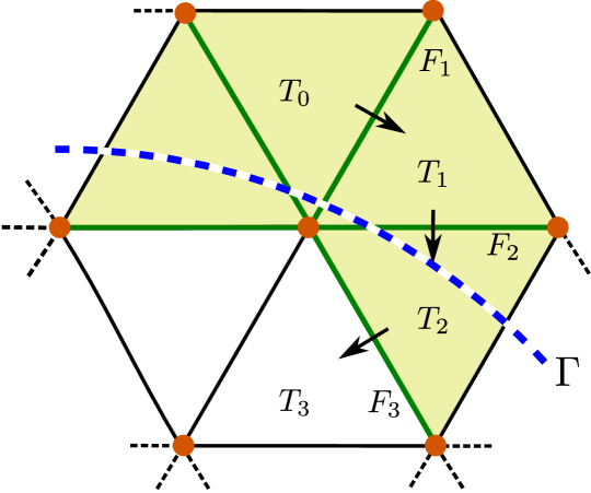
Fig. 5.1: Controlling the $L^{2}$-norm $\|v\|_{T_{0}}$ of a finite element function $v$ on a barely intersected, “fictitious” element $T_{0}$ by $\|v\|_{T_{3}}$ and boundary zone jump-penalties. Starting from $T_{0}$, each term $\|v\|_{T_{i}}^{2}$ can be estimated by the neighboring term $\|v\|_{T_{i+1}^{2}}$ when a sum of jump-terms of the form $h_{F_{i+1}}^{2j+i}\|\partial_{\boldsymbol{n}}v\|_{F_{i+1}}^{2}$ is added.

As a first step, we show how the jump-penalties (3.11) and (3.12) in the boundary zone $\mathcal{F}^{\ast}_{\Gamma}$ contribute to control the norms of $\boldsymbol{v}_{h}$ and $p_{h}$ on the entire fictitious domain $\mathcal{T}^{\ast}$. We start with the following lemma.

Lemma 5.1.

Let $\mathcal{T}=\{T\}$ be a tessellation consisting of shape-regular elements $T$ and let $T_{1},\,T_{2}\in\mathcal{T}$ be two elements sharing a common face $F$. Furthermore, let $v$ be a piecewise polynomial function defined relative to the macro-element $\overline{T}=T_{1}\cup T_{2}$. Let $v_{i}$ be the restriction of $v$ to $T_{i}$ for $i=1,2$. Then there is a constant $C>0$, depending only on the shape-regularity of $\mathcal{T}$ and the polynomial order $p=\max(\operatorname{ord}(v_{1}),\operatorname{ord}(v_{2}))$ of $v$, such that

$$\|v\|_{T_{1}}^{2}\leqslant C\left(\|v\|_{T_{2}}^{2}+\sum_{j\leqslant p}h^{2j+1}([\partial_{\boldsymbol{n}}^{j}v],[\partial_{\boldsymbol{n}}^{j}v])_{F}\right),$$ (5.1)

where $\partial_{\boldsymbol{n}}^{j}v=\sum_{|\alpha|=j}D^{\alpha}v(\boldsymbol{x})\boldsymbol{n}^{\alpha}$ for multi-index $\alpha=(\alpha_{1},\ldots,\alpha_{d})$, $|\alpha|=\sum_{i}\alpha_{i}$ and $\boldsymbol{n}^{\alpha}=n_{1}^{\alpha_{1}}n_{2}^{\alpha_{2}}\cdots n_{d}^{\alpha_{d}}$.

Proof.

For a given point $\boldsymbol{x}\in T_{1}$, we write $\boldsymbol{x}_{F}=\boldsymbol{x}_{F}(\boldsymbol{x})$ for the normal projection of $\boldsymbol{x}$ onto the plane defined by the face $F$. Note that the area $|T_{1,F}|$ of all projected points in $T_{1}$ is bounded by $|F|$ up to a constant by the shape-regularity assumption. For $i=1,2$, and since $\operatorname{ord}(v_{i})\leqslant p$, we may express (the extensions to $\overline{T}$ of) $v_{i}$ in terms of its Taylor-expansion around $\boldsymbol{x}_{F}$:

$$v_{i}(\boldsymbol{x})=\sum_{|\alpha|\leqslant p}\dfrac{D^{\alpha}v_{i}(\boldsymbol{x}_{F})}{\alpha!}(|\boldsymbol{x}-\boldsymbol{x}_{F}|\boldsymbol{n})^{\alpha},$$

where $\boldsymbol{n}$ is the unit normal vector of $F$ pointing towards $T_{1}$. Subtracting the two Taylor expansions, we find that

$$v_{1}(\boldsymbol{x})=v_{2}(\boldsymbol{x})+\sum_{|\alpha|\leqslant p}\dfrac{[D^{\alpha}v(\boldsymbol{x}_{F})]}{\alpha!}(|\boldsymbol{x}-\boldsymbol{x}_{F}|\boldsymbol{n})^{\alpha}.$$

Next, integrating over $T_{1}$ with respect to $\boldsymbol{x}$, taking squares and applying the Cauchy–Schwarz inequality yield

$$\|v_{1}\|_{T_{1}}^{2}\leqslant C\left(\|v_{2}\|_{T_{1}}^{2}+\sum_{|\alpha|\leqslant p}\int_{T_{1}}\left([D^{\alpha}v(\boldsymbol{x}_{F}(\boldsymbol{x}))]\boldsymbol{n}^{\alpha}\right)^{2}h^{2|\alpha|}\,\mathrm{d}x\right),$$

with $h$ the maximal element diameter. From the assumption of shape regularity, a change of variables, and the definition of $\partial_{\boldsymbol{n}}^{j}$, it follows that

$$\|v_{1}\|_{T_{1}}^{2}\leqslant C\left(\|v_{2}\|_{T_{1}}^{2}+\sum_{j\leqslant p}\int_{F}{[\partial_{\boldsymbol{n}}^{j}v(y)]^{2}}h^{2j+1}\,\mathrm{d}y\right).$$

Finally, as the two norms $\|v_{2}\|_{T_{1}}$ and $\|v_{2}\|_{T_{2}}$ are equivalent, again by shape regularity, we obtain the desired inequality (5.1). ∎

Remark 5.1.

The previous lemma is a key observation for proving stability and a priori error estimates for the fictitious domain formulation (3.13) as it lays the foundation for how to control certain norms on the fictitious domain $\Omega^{\ast}$ in terms of norms computed only on $\Omega$ and appropriate jump-penalties in the intersection zone $\mathcal{F}^{\ast}_{\Gamma}$.

We are now in a position to state the following proposition:

Proposition 5.1.

Let $\Omega$, $\Omega^{\ast}$ and $\mathcal{F}^{\ast}_{\Gamma}$ be defined as in Section 2.1. There is a constant $C>0$ such that the following estimates hold.
For all $\boldsymbol{v}_{h}\in V_{h}(\mathcal{T}^{\ast})$:

$$\|\nabla\boldsymbol{v}_{h}\|_{\Omega^{\ast}}^{2}\leqslant C\bigl{(}\|\nabla\boldsymbol{v}_{h}\|_{\Omega}^{2}+\sum_{F\in\mathcal{F}^{\ast}_{\Gamma}}h_{F}([\partial_{\boldsymbol{n}}\boldsymbol{v}_{h}],[\partial_{\boldsymbol{n}}\boldsymbol{v}_{h}])_{F}\bigr{)}\leqslant C\|\nabla\boldsymbol{v}_{h}\|_{\Omega^{\ast}}^{2}$$ (5.2)

and for all $q_{h}\in P_{h}^{0,\mathrm{dc}}(\mathcal{T}^{\ast})$:

$$\|q_{h}\|_{\Omega^{\ast}}^{2}\leqslant C\bigl{(}\|q_{h}\|_{\Omega}^{2}+\sum_{F\in\mathcal{F}^{\ast}_{\Gamma}}h_{F}([\boldsymbol{n}\cdot q_{h}],[\boldsymbol{n}\cdot q_{h}])_{F}\bigr{)}\leqslant C\|q_{h}\|_{\Omega^{\ast}}^{2}$$ (5.3)

while, for all $q_{h}\in P_{h}^{1}(\mathcal{T}^{\ast})$:

$$\|q_{h}\|_{\Omega^{\ast}}^{2}\leqslant C\bigl{(}\|q_{h}\|_{\Omega}^{2}+\sum_{F\in\mathcal{F}^{\ast}_{\Gamma}}h_{F}^{3}([\partial_{\boldsymbol{n}}q_{h}],[\partial_{\boldsymbol{n}}q_{h}])_{F}\bigr{)}\leqslant C\|q_{h}\|_{\Omega^{\ast}}^{2}.$$ (5.4)

Proof.

We start with the first inequality of (5.2). Decompose the norm over $\Omega^{\ast}$ into sums over non-cut and cut elements. Let $T_{0}\in\mathcal{T}^{\ast}_{\Gamma}$ be a cut element. By the geometric condition G3 (cf. Section 2.1), there exists a $T_{N}\subset\Omega$ and at most $N-1$ elements $T_{i}\in\mathcal{T}^{\ast}_{\Gamma}$ and facets $T_{i-1}\cap T_{i}=F_{i}\in\mathcal{F}^{\ast}_{\Gamma}$ that have to be crossed in order to traverse from $T_{0}$ to $T_{N}$. By the shape-regularity of the mesh, each facet $F\in\mathcal{F}^{\ast}_{\Gamma}$ will only be involved in a finite number of such crossings. Applying Lemma 5.1, with each component of $\nabla\boldsymbol{v}_{h}$ as $v$, iteratively to each neighboring pair $\{T_{i-1},T_{i}\}$ yields the desired estimate.

The first inequalities of (5.3) and (5.4) follow by the analogous argument: apply Lemma 5.1 to $q_{h}$ and recall that $[q_{h}]_{F}=0$ for $q_{h}\in P_{h}^{1}$.

The second inequalities of (5.2)–(5.4) rely on the shape regularity, allowing us to bound $h_{F}$ by $h$, and the trace and inverse estimates of Section 4.1 applied to each facet of the boundary zone sums. The upper bounds immediately follow. ∎

Remark 5.2.

Burman and Hansbo [11] presented the analogous result to (5.2) for the Poisson problem with continuous piecewise linear finite elements. The formulation given here, together with Lemma 5.1, reveals the basic structure of jump-penalty-based stabilization terms for fictitious domain formulations and can be applied to various types of norms and elements, including higher-order elements.

5.2 Stability estimates and the inf-sup condition

The main result of this section, Theorem 5.16, is the inf-sup stability of the bilinear form $A_{h}+J_{h}$, occurring in the stabilized Nitsche fictitious domain variational formulation (3.13), with respect to the $|\mspace{-1.0mu}|\mspace{-1.0mu}|\cdot|\mspace{-1.0mu}|\mspace{-1.0mu}|_{*}$ norm (2.9).

We begin by establishing the properties of the separate contributions to the bilinear form. First, the form $a_{h}$ cf. (3.9) augmented by $i_{h}$ cf. (3.11) is continuous and coercive with respect to the norms $|\mspace{-1.0mu}|\mspace{-1.0mu}|\cdot|\mspace{-1.0mu}|\mspace{-1.0mu}|$ and $|\mspace{-1.0mu}|\mspace{-1.0mu}|\cdot|\mspace{-1.0mu}|\mspace{-1.0mu}|_{\ast}$ [11]. More precisely, there are constants $c>0$ and $C>0$ such that

$$a_{h}(\boldsymbol{v},\boldsymbol{w}) \leqslant C|\mspace{-1.0mu}|\mspace{-1.0mu}|\boldsymbol{v}|\mspace{-1.0mu}|\mspace{-1.0mu}|\;|\mspace{-1.0mu}|\mspace{-1.0mu}|\boldsymbol{w}|\mspace{-1.0mu}|\mspace{-1.0mu}|\quad\forall\,\boldsymbol{v},\boldsymbol{w}\in[H^{1}(\mathcal{T})]^{d},$$ (5.5)

$$a_{h}(\boldsymbol{v}_{h},\boldsymbol{w}_{h})+i_{h}(\boldsymbol{v}_{h},\boldsymbol{w}_{h}) \leqslant C|\mspace{-1.0mu}|\mspace{-1.0mu}|\boldsymbol{v}_{h}|\mspace{-1.0mu}|\mspace{-1.0mu}|_{\ast}\;|\mspace{-1.0mu}|\mspace{-1.0mu}|\boldsymbol{w}_{h}|\mspace{-1.0mu}|\mspace{-1.0mu}|_{\ast}\quad\forall\,\boldsymbol{v}_{h},\boldsymbol{w}_{h}\in V_{h}(\mathcal{T}^{\ast}),$$ (5.6)

$$c|\mspace{-1.0mu}|\mspace{-1.0mu}|\boldsymbol{w}_{h}|\mspace{-1.0mu}|\mspace{-1.0mu}|_{\ast}^{2} \leqslant a_{h}(\boldsymbol{w}_{h},\boldsymbol{w}_{h})+i_{h}(\boldsymbol{w}_{h},\boldsymbol{w}_{h})\quad\forall\,\boldsymbol{w}_{h}\in V_{h}(\mathcal{T}^{\ast}).$$ (5.7)

Next, we show that $b_{h}$ is continuous with respect to the relevant norms.

Proposition 5.2.

Let $b_{h}$ be defined by (3.10). There is a constant $C>0$ such that

$$b_{h}(\boldsymbol{v},q) \leqslant C|\mspace{-1.0mu}|\mspace{-1.0mu}|\boldsymbol{v}|\mspace{-1.0mu}|\mspace{-1.0mu}|\,|\mspace{-1.0mu}|\mspace{-1.0mu}|q|\mspace{-1.0mu}|\mspace{-1.0mu}| \forall\,(\boldsymbol{v},q)\in[H^{1}_{0}(\Omega)]^{d}\times L^{2}(\Omega),$$ (5.8)

$$b_{h}(\boldsymbol{v}_{h},q_{h}) \leqslant C|\mspace{-1.0mu}|\mspace{-1.0mu}|\boldsymbol{v}_{h}|\mspace{-1.0mu}|\mspace{-1.0mu}|_{\ast}|\mspace{-1.0mu}|\mspace{-1.0mu}|q_{h}|\mspace{-1.0mu}|\mspace{-1.0mu}|_{\ast} \forall\,(\boldsymbol{v}_{h},q_{h})\in V_{h}(\mathcal{T}^{\ast})\times Q_{h}(\mathcal{T}^{\ast}).$$ (5.9)

Proof.

The bound (5.9) follows from the definitions of $b_{h}$ and the $|\mspace{-1.0mu}|\mspace{-1.0mu}|~{}\cdot~{}|\mspace{-1.0mu}|\mspace{-1.0mu}|_{\ast}$ norm, and a subsequent use of (4.2) and (4.3). ∎

The next lemma gives a fictitious domain adapted version of a “bad inequality” often used in Verfürth’s trick [36] and in proofs for some classical, stabilized schemes [14].

Lemma 5.2.

There are positive constants $C_{1},C_{2}$ such that for each $q_{h}\in Q_{h}(\mathcal{T})$ there exists a $\boldsymbol{v}_{h}\in V_{h}(\mathcal{T}^{\ast})$ satisfying

$$\frac{b_{h}(\boldsymbol{v}_{h},q_{h})}{|\mspace{-1.0mu}|\mspace{-1.0mu}|\boldsymbol{v}_{h}|\mspace{-1.0mu}|\mspace{-1.0mu}|_{\ast}}\geqslant C_{1}\|q_{h}\|_{\Omega}-C_{2}\big{(}(\sum_{T\in\mathcal{T}}h_{T}^{2}\|\nabla q_{h}\|_{T}^{2})^{1/2}+(\sum_{F\in\partial_{i}\mathcal{T}}h_{F}\|[q_{h}]\|_{F}^{2})^{1/2}\big{)}.$$ (5.10)

Proof.

Let $q_{h}\in Q_{h}(\mathcal{T})$ be given. There exists a $\boldsymbol{v}\in[H^{1}(\Omega)]^{d}$ and a constant $\widetilde{C}_{1}>0$ such that $\operatorname{div}\boldsymbol{v}=q_{h}$ and $\widetilde{C}_{1}\|\boldsymbol{v}\|_{1,\Omega}\leqslant\|\operatorname{div}\boldsymbol{v}\|_{\Omega}$ [15]. Map $\boldsymbol{v}\mapsto\pi_{h}\boldsymbol{v}\in V_{h}(\mathcal{T}^{\ast})$ by the extended interpolation operator cf. (4.10), and denote $\boldsymbol{e}_{h}=\pi_{h}\boldsymbol{v}-\boldsymbol{v}$. It follows, using the definition of $b_{h}$, that

$$b_{h}(\pi_{h}\boldsymbol{v},q_{h})=b_{h}(\boldsymbol{e}_{h},q_{h})+b_{h}(\boldsymbol{v},q_{h})\geqslant b_{h}(\boldsymbol{e}_{h},q_{h})+\widetilde{C}_{1}\|\boldsymbol{v}\|_{1,\Omega}\|q_{h}\|_{\Omega}.$$ (5.11)

Moreover, integrating by parts on each element $T\in\mathcal{T}$ yields

$$\begin{split}b_{h}(\boldsymbol{e}_{h},q_{h})&=-(\operatorname{div}\boldsymbol{e}_{h},q_{h})_{\Omega}+(\boldsymbol{n}\cdot\boldsymbol{e}_{h},q_{h})_{\Gamma}\\ &=\sum_{T\in\mathcal{T}}(\boldsymbol{e}_{h},\nabla q_{h})_{T}+\sum_{F\in\partial_{i}\mathcal{T}}(\boldsymbol{n}\cdot\boldsymbol{e}_{h},[q_{h}])_{F},\end{split}$$ (5.12)

while the Cauchy-Schwarz inequalities give

$$\sum_{T\in\mathcal{T}}(\boldsymbol{e}_{h},\nabla q_{h})_{T} \geqslant-(\sum_{T\in\mathcal{T}}h_{T}^{-2}\|\boldsymbol{e}_{h}\|^{2}_{T})^{1/2}(\sum_{T\in\mathcal{T}}h_{T}^{2}\|\nabla q_{h}\|_{T}^{2})^{1/2},$$ (5.13)

$$\sum_{F\in\partial_{i}\mathcal{T}}(\boldsymbol{n}\cdot\boldsymbol{e}_{h},[q_{h}])_{F} \geqslant-(\sum_{F\in\partial_{i}\mathcal{T}}h_{F}^{-1}\|\boldsymbol{e}_{h}\|^{2}_{F})^{1/2}(\sum_{F\in\partial_{i}\mathcal{T}}h_{F}\|[q_{h}]\|_{F}^{2})^{1/2}.$$ (5.14)

Since $h_{T}^{-1}\|\boldsymbol{e}_{h}\|_{T}\leqslant C\|\boldsymbol{v}\|_{1,\omega(T)}$ by (4.11) and $h_{F}^{-1/2}\|\boldsymbol{e}_{h}\|_{F}\leqslant C\|\boldsymbol{v}\|_{1,\omega(T)}$ by (4.12), we obtain by combining (5.12) with (5.13) and (5.14):

$$\begin{split}b_{h}(\boldsymbol{e}_{h},q_{h})\geqslant-\widetilde{C}_{2}\|\boldsymbol{v}\|_{1,\Omega}\left((\sum_{T\in\mathcal{T}}h_{T}^{2}\|\nabla q_{h}\|_{T}^{2})^{1/2}+(\sum_{F\in\partial_{i}\mathcal{T}}h_{F}\|[q_{h}]\|_{F}^{2})^{1/2}\right)\end{split}$$ (5.15)

Finally, combining (5.11) with (5.15), and recalling that $|\mspace{-1.0mu}|\mspace{-1.0mu}|\pi_{h}\boldsymbol{v}|\mspace{-1.0mu}|\mspace{-1.0mu}|_{\ast}\leqslant C\|\boldsymbol{v}\|_{1,\Omega}$ by Lemma 4.2, yields (5.10) with $\boldsymbol{v}_{h}=\pi_{h}\boldsymbol{v}$. ∎

Using the stability estimates for $a_{h}$ and $b_{h}$, we may now prove the following inf-sup stability estimate for for $A_{h}+J_{h}$:

Theorem 5.1.

There is a constant $c_{A}>0$ such that for all $(\boldsymbol{u}_{h},p_{h})\in V_{h}\times Q_{h}=V_{h}(\mathcal{T}^{\ast})\times Q_{h}(\mathcal{T}^{\ast})$:

$$\sup_{(\boldsymbol{v}_{h},q_{h})\in V_{h}\times Q_{h}}\frac{A_{h}(\boldsymbol{u}_{h},p_{h};\boldsymbol{v}_{h},q_{h})+J_{h}(\boldsymbol{u}_{h},p_{h};\boldsymbol{v}_{h},q_{h})}{|\mspace{-1.0mu}|\mspace{-1.0mu}|(\boldsymbol{v}_{h},q_{h})|\mspace{-1.0mu}|\mspace{-1.0mu}|_{\ast}}\geqslant c_{A}|\mspace{-1.0mu}|\mspace{-1.0mu}|(\boldsymbol{u}_{h},p_{h})|\mspace{-1.0mu}|\mspace{-1.0mu}|_{\ast}.$$ (5.16)

Proof.

The proof of Theorem 5.16 follows the proof by Franca et al. [14], using the appropriate norms and Proposition 5.1 in combination with Lemma 5.2. Let $(\boldsymbol{u}_{h},p_{h})$ be given.

First, choose $(\boldsymbol{v}_{h},q_{h})$ to be $(-\boldsymbol{w}_{h},0)$ where $-\boldsymbol{w}_{h}$ satisfies (5.10) for the given $p_{h}$. In addition, scale $\boldsymbol{w}_{h}$ such that $|\mspace{-1.0mu}|\mspace{-1.0mu}|\boldsymbol{w}_{h}|\mspace{-1.0mu}|\mspace{-1.0mu}|_{\ast}=\|p_{h}\|_{\Omega}$. For the sake of readability, we write

$$k_{\mathcal{T}}(p_{h})\equiv(\sum_{T\in\mathcal{T}}h_{T}^{2}\|\nabla p_{h}\|_{T}^{2})^{1/2}+(\sum_{F\in\partial_{i}\mathcal{T}}h_{F}\|[p_{h}]\|_{F}^{2})^{1/2}.$$ (5.17)

With this choice of test functions, applying (5.6) and (5.10), and Cauchy’s inequality with $\epsilon$ give

$$(A_{h}+J_{h}) (\boldsymbol{u}_{h},p_{h};-\boldsymbol{w}_{h},0)=-a_{h}(\boldsymbol{u}_{h},\boldsymbol{w}_{h})-i_{h}(\boldsymbol{u}_{h},\boldsymbol{w}_{h})+b_{h}(\boldsymbol{w}_{h},-p_{h})$$

$$\geqslant-C|\mspace{-1.0mu}|\mspace{-1.0mu}|\boldsymbol{u}_{h}|\mspace{-1.0mu}|\mspace{-1.0mu}|_{\ast}\,\|p_{h}\|_{\Omega}+C_{1}\|p_{h}\|_{\Omega}^{2}-C_{2}k_{\mathcal{T}}(p_{h})\,\|p_{h}\|_{\Omega}$$

$$\geqslant-\frac{C}{4\epsilon}|\mspace{-1.0mu}|\mspace{-1.0mu}|\boldsymbol{u}_{h}|\mspace{-1.0mu}|\mspace{-1.0mu}|_{\ast}^{2}+\left(C_{1}-\epsilon(C+C_{2})\right)||p_{h}||_{\Omega}^{2}-\frac{C_{2}}{4\epsilon}k_{\mathcal{T}}(p_{h})^{2}.$$

Note that by definition $k_{\mathcal{T}}(p_{h})^{2}\leqslant Kc_{h}(p_{h},p_{h})$ for some positive constant $K$ depending on $\beta_{0}$ and $\beta_{1}$. In combination with choosing $\epsilon$ such that $(C_{1}-\epsilon(C+C_{2}))>0$, this gives

$$(A_{h}+J_{h})(\boldsymbol{u}_{h},p_{h};-\boldsymbol{w}_{h},0)\geqslant-\tilde{C}|\mspace{-1.0mu}|\mspace{-1.0mu}|\boldsymbol{u}_{h}|\mspace{-1.0mu}|\mspace{-1.0mu}|_{\ast}^{2}+\tilde{C}_{1}\|p_{h}\|_{\Omega}^{2}-\tilde{C}_{2}c_{h}(p_{h},p_{h}).$$

Second, we take test functions $(\boldsymbol{v}_{h},q_{h})=(\boldsymbol{u}_{h},-p_{h})$ which, using (5.7), gives

$$(A_{h}+J_{h})(\boldsymbol{u}_{h},p_{h};\boldsymbol{u}_{h},-p_{h}) =a_{h}(\boldsymbol{u}_{h},\boldsymbol{u}_{h})+i_{h}(\boldsymbol{u}_{h},\boldsymbol{u}_{h})+c_{h}(p_{h},p_{h})+j_{h}(p_{h},p_{h})$$

$$\geqslant c|\mspace{-1.0mu}|\mspace{-1.0mu}|\boldsymbol{u}_{h}|\mspace{-1.0mu}|\mspace{-1.0mu}|_{\ast}^{2}+c_{h}(p_{h},p_{h})+j_{h}(p_{h},p_{h}).$$

In total, for any $\delta>0$, we have

$$(A_{h}+J_{h}) (\boldsymbol{u}_{h},p_{h};\boldsymbol{u}_{h},-p_{h})+\delta(A_{h}+J_{h})(\boldsymbol{u}_{h},p_{h};-\boldsymbol{w}_{h},0)$$

$$\geqslant(c-\delta\tilde{C})|\mspace{-1.0mu}|\mspace{-1.0mu}|\boldsymbol{u}_{h}|\mspace{-1.0mu}|\mspace{-1.0mu}|_{\ast}^{2}+(1-\delta\tilde{C}_{2})c_{h}(p_{h},p_{h})+\delta\tilde{C}_{1}\|p_{h}\|_{\Omega}^{2}+j_{h}(p_{h},p_{h}).$$

Moreover, by (5.3) and (5.4), there exists a positive constant $D$ such that

$$\|p_{h}\|_{\Omega}^{2}+j_{h}(p_{h},p_{h})\geqslant D\|p_{h}\|_{\Omega^{\ast}}^{2}\equiv D|\mspace{-1.0mu}|\mspace{-1.0mu}|p_{h}|\mspace{-1.0mu}|\mspace{-1.0mu}|_{\ast}^{2}.$$ (5.18)

Finally, we conclude that by a suitable choice of $\delta>0$, there is a positive constant $c_{A}$ such that $(\boldsymbol{v}_{h},q_{h})=(\boldsymbol{u}_{h}-\delta\boldsymbol{w}_{h},-p_{h})$ satisfies

$$(A_{h}+J_{h})(\boldsymbol{u}_{h},p_{h};\boldsymbol{v},q_{h})\geqslant c_{A}(|\mspace{-1.0mu}|\mspace{-1.0mu}|\boldsymbol{u}_{h}|\mspace{-1.0mu}|\mspace{-1.0mu}|_{\ast}^{2}+|\mspace{-1.0mu}|\mspace{-1.0mu}|p_{h}|\mspace{-1.0mu}|\mspace{-1.0mu}|_{\ast}^{2}),$$

which proves the desired estimate. ∎

6 A priori error estimate

Before we formulate the main a priori error estimate, we state two lemmas about how the stabilization form $J_{h}$ affects the Galerkin orthogonality and the consistency of the total form $A_{h}+J_{h}$. Let $V_{h}=V_{h}(\mathcal{T}^{\ast})$ and $Q_{h}=Q_{h}(\mathcal{T}^{\ast})$ throughout this section.

Lemma 6.1.

(Weak Galerkin orthogonality). Let $(\boldsymbol{u},p)\in[H^{2}(\Omega)]^{d}\times H^{1}(\Omega)$ be the solution of the Stokes problem (1.1) and let $(\boldsymbol{u}_{h},p_{h})$ be the discrete solution of the corresponding stabilized Nitsche fictitious domain formulation (3.13). Then,

$$A_{h}(\boldsymbol{u}-\boldsymbol{u}_{h},p-p_{h};\boldsymbol{v}_{h},q_{h})-J_{h}(\boldsymbol{u}_{h},p_{h};\boldsymbol{v}_{h},q_{h})=0\quad\forall\,(\boldsymbol{v}_{h},q_{h})\in V_{h}\times Q_{h}.$$ (6.1)

Proof.

The identify follows immediately from the fact that the solution $(\boldsymbol{u},p)$ satisfies $A_{h}(\boldsymbol{u},p;\boldsymbol{v}_{h},q_{h})=L_{h}(\boldsymbol{v}_{h},q_{h})$, as defined by (3.14) and (3.16), for all $(\boldsymbol{v}_{h},q_{h})\in V_{h}\times Q_{h}$. ∎

The ghost penalty part $j_{1,h}$ in $J_{h}$ involves the evaluation of $\partial_{\boldsymbol{n}}q_{h}$ on facets and therefore the variational formulation (3.13) is per se not consistent with (1.1) since we only assume that $q\in H^{1}(\Omega)$. The next lemma shows that this consistency error will not affect the convergence order.

Lemma 6.2.

(Weak consistency) Assume that $\boldsymbol{u}\in[H^{2}(\Omega)]^{d}$ and $p\in H^{1}(\Omega)$ and let $\pi_{h}$ be the interpolation operator defined by (4.10). Then for all $(\boldsymbol{v}_{h},q_{h})\in V_{h}\times Q_{h}$ it holds that

$$J_{h}(\pi_{h}\boldsymbol{u},\pi_{h}p;\boldsymbol{v}_{h},q_{h})\leqslant Ch(|\boldsymbol{u}|_{2,\Omega}+|p|_{1,\Omega})|\mspace{-1.0mu}|\mspace{-1.0mu}|(\boldsymbol{v}_{h},q_{h})|\mspace{-1.0mu}|\mspace{-1.0mu}|_{\ast}.$$ (6.2)

Proof.

By definition (3.15):

$$J_{h}(\pi_{h}\boldsymbol{u},\pi_{h}p;\boldsymbol{v}_{h},q_{h})=i_{h}(\pi_{h}\boldsymbol{u},\boldsymbol{v}_{h})-j_{h,0}(\pi_{h}p,q_{h})-j_{h,1}(\pi_{h}p,q_{h}).$$

By the continuity assumption on $\boldsymbol{u}$, $i_{h}(\mathcal{E}\boldsymbol{u},\boldsymbol{v}_{h})=0$. So, by the definition of $\pi_{h}$ (4.10), the inverse inequality (4.4) and the interpolation estimate (4.8), and the continuity of $\mathcal{E}$, we obtain

$$i_{h}(\pi_{h}\boldsymbol{u},\boldsymbol{v}_{h})=i_{h}(\pi^{\ast}_{h}\mathcal{E}\boldsymbol{u}-\mathcal{E}\boldsymbol{u},\boldsymbol{v}_{h})\leqslant Ch|\mathcal{E}\boldsymbol{u}|_{2,\Omega^{\ast}}\|\nabla\boldsymbol{v}_{h}\|_{\Omega^{\ast}}\leqslant Ch|\boldsymbol{u}|_{2,\Omega}|\mspace{-1.0mu}|\mspace{-1.0mu}|\boldsymbol{v}_{h}|\mspace{-1.0mu}|\mspace{-1.0mu}|_{\ast}.$$

Similarly, by the continuity assumption on $p$; the trace inequality (4.1), the inverse estimate (4.3) and the interpolation estimate (4.9); and the continuity of $\mathcal{E}$:

$$j_{h,0}(\pi_{h}p,q_{h})=j_{h,0}(\pi^{\ast}_{h}\mathcal{E}p-\mathcal{E}p,q_{h})\leqslant Ch|\mathcal{E}p|_{1,\Omega^{\ast}}\|q_{h}\|_{\Omega^{\ast}}\leqslant Ch|p|_{1,\Omega}|\mspace{-1.0mu}|\mspace{-1.0mu}|q_{h}|\mspace{-1.0mu}|\mspace{-1.0mu}|_{\ast}.$$

Finally, to estimate $j_{h,1}$, we use (4.4) and (4.3); the boundedness of the Scott–Zhang interpolant, and the continuity of $\mathcal{E}$ to obtain

$$j_{h,1}(\pi_{h}p,q_{h})\leqslant Ch\|\nabla\pi_{h}p\|_{\Omega^{\ast}}\|q\|_{\Omega^{\ast}}\leqslant Ch|p|_{1,\Omega}|\mspace{-1.0mu}|\mspace{-1.0mu}|q_{h}|\mspace{-1.0mu}|\mspace{-1.0mu}|_{\ast}.$$

Combining the three estimates yields the result (6.2). ∎

Theorem 6.1.

(A priori error estimate) Let $(\boldsymbol{u},p)\in[H^{2}(\Omega)]^{d}\times H^{1}(\Omega)$ be the solution of the Stokes problem (1.1) and let $(\boldsymbol{u}_{h},p_{h})$ be the discrete solution of the corresponding stabilized Nitsche fictitious domain formulation (3.13). Then, there is a constant $C>0$ such that

$$|\mspace{-1.0mu}|\mspace{-1.0mu}|(\boldsymbol{u}-\boldsymbol{u}_{h},p-p_{h})|\mspace{-1.0mu}|\mspace{-1.0mu}|\leqslant Ch\left(|\boldsymbol{u}|_{2,\Omega}+|p|_{1,\Omega}\right).$$ (6.3)

Proof.

Clearly, by the triangle inequality and (4.6):

$$|\mspace{-1.0mu}|\mspace{-1.0mu}|(\boldsymbol{u}-\boldsymbol{u}_{h},p-p_{h})|\mspace{-1.0mu}|\mspace{-1.0mu}|\leqslant|\mspace{-1.0mu}|\mspace{-1.0mu}|(\boldsymbol{u}-\pi_{h}\boldsymbol{u},p-\pi_{h}p)|\mspace{-1.0mu}|\mspace{-1.0mu}|+C|\mspace{-1.0mu}|\mspace{-1.0mu}|(\pi_{h}\boldsymbol{u}-\boldsymbol{u}_{h},\pi_{h}p-p_{h})|\mspace{-1.0mu}|\mspace{-1.0mu}|_{\ast}.$$

Lemma 4.1 provides the desired bound for the first term on the right-hand side above. It is therefore enough to show that the discrete error $(\pi_{h}\boldsymbol{u}-\boldsymbol{u}_{h},\pi_{h}p-p_{h})$ satisfies the error bound in (6.3).

By Theorem 5.16, there exists a $(\boldsymbol{v}_{h},p_{h})$ such that $|\mspace{-1.0mu}|\mspace{-1.0mu}|(\boldsymbol{v}_{h},p_{h})|\mspace{-1.0mu}|\mspace{-1.0mu}|_{\ast}=1$ and

$$c_{A}|\mspace{-1.0mu}|\mspace{-1.0mu}|(\pi_{h}\boldsymbol{u}-\boldsymbol{u}_{h},\pi_{h}p-p_{h})|\mspace{-1.0mu}|\mspace{-1.0mu}|_{\ast}\\ \leqslant A_{h}(\boldsymbol{u}_{h}-\pi_{h}\boldsymbol{u},p_{h}-\pi_{h}p;\boldsymbol{v}_{h},q_{h})+J_{h}(\boldsymbol{u}_{h}-\pi_{h}\boldsymbol{u},p_{h}-\pi_{h}p;\boldsymbol{v}_{h},q_{h})\\ =A_{h}(\boldsymbol{u}-\pi_{h}\boldsymbol{u};p-\pi_{h}p;\boldsymbol{v}_{h},q_{h})-J_{h}(\pi_{h}\boldsymbol{u},\pi_{h}p;\boldsymbol{v}_{h},q_{h}),$$

where the last equality follows by the weak Galerkin orthogonality (6.1). Recalling the definition of $A_{h}$, we may write

$$A_{h}(\boldsymbol{u}-\pi_{h}\boldsymbol{u},p-\pi_{h}p;\boldsymbol{v}_{h},q_{h}) =a_{h}(\boldsymbol{u}-\pi_{h}\boldsymbol{u},\boldsymbol{v}_{h})$$

$$\quad+b_{h}(\boldsymbol{u}-\pi_{h}\boldsymbol{u},q_{h})+b_{h}(\boldsymbol{v}_{h},p-\pi_{h}p)$$

$$\quad+c_{h}(\boldsymbol{u}-\pi_{h}\boldsymbol{u};p-\pi_{h}p,q_{h}).$$

We use the stability estimate (5.5) for $a_{h}$ and (5.8) for $b_{h}$; and (4.6) and (4.14) to estimate the first three terms:

$$a_{h}(\boldsymbol{u}-\pi_{h}\boldsymbol{u},\boldsymbol{v}_{h})+b_{h}(\boldsymbol{u}-\pi_{h}\boldsymbol{u},q_{h})+b_{h}(\boldsymbol{v}_{h},p-\pi_{h}p)$$

$$\qquad\leqslant C\bigl{(}|\mspace{-1.0mu}|\mspace{-1.0mu}|\boldsymbol{u}-\pi_{h}\boldsymbol{u}|\mspace{-1.0mu}|\mspace{-1.0mu}|\;|\mspace{-1.0mu}|\mspace{-1.0mu}|\boldsymbol{v}_{h}|\mspace{-1.0mu}|\mspace{-1.0mu}|_{\ast}+|\mspace{-1.0mu}|\mspace{-1.0mu}|\boldsymbol{u}-\pi_{h}\boldsymbol{u}|\mspace{-1.0mu}|\mspace{-1.0mu}|\;|\mspace{-1.0mu}|\mspace{-1.0mu}|q_{h}|\mspace{-1.0mu}|\mspace{-1.0mu}|_{\ast}+|\mspace{-1.0mu}|\mspace{-1.0mu}|\boldsymbol{v}_{h}|\mspace{-1.0mu}|\mspace{-1.0mu}|_{\ast}\;|\mspace{-1.0mu}|\mspace{-1.0mu}|p-\pi_{h}p|\mspace{-1.0mu}|\mspace{-1.0mu}|\bigr{)}$$

$$\qquad\leqslant Ch\bigl{(}|\boldsymbol{u}|_{2,\Omega}+|p|_{1,\Omega}\bigr{)}|\mspace{-1.0mu}|\mspace{-1.0mu}|(\boldsymbol{v}_{h},q_{h})|\mspace{-1.0mu}|\mspace{-1.0mu}|_{\ast}.$$

Using the fact that $\Delta\pi_{h}\boldsymbol{u}=0$ locally and applying the Cauchy–Schwarz inequality, we may estimate the remaining term $c_{h}=c_{h}(\boldsymbol{u}-\pi_{h}\boldsymbol{u};p-\pi_{h}p,q_{h})$ by

$$c_{h} =\beta_{0}\sum_{F\in\partial_{i}\mathcal{T}}h_{F}([p-\pi_{h}p],[q_{h}])_{F}+\beta_{1}\sum_{T\in\mathcal{T}}h_{T}^{2}(-\Delta\boldsymbol{u}+\nabla(p-\pi_{h}p_{h}),\nabla q_{h})_{T}$$

$$\leqslant C\Bigl{(}\bigl{(}\sum_{T\in\mathcal{T}}h_{T}^{2}\|\Delta\boldsymbol{u}\|_{T}^{2}\bigr{)}^{1/2}+\bigl{(}\sum_{T\in\mathcal{T}}h_{T}^{2}\|\nabla(p-\pi_{h}p)\|_{T}^{2}\bigr{)}^{1/2}\Bigr{)}\Bigl{(}\sum_{T\in\mathcal{T}^{\ast}}h_{T}^{2}\|\nabla q_{h}\|_{T}^{2}\Bigr{)}^{1/2}$$

$$\quad+C\bigl{(}\sum_{F\in\partial_{i}\mathcal{T}}h_{F}\|[p-\pi_{h}p]\|_{F}^{2}\bigr{)}^{1/2}\Bigr{)}\Bigl{(}\sum_{F\in\partial_{i}\mathcal{T}^{\ast}}h_{F}\|[q_{h}]\|_{F}^{2}\Bigr{)}^{1/2}$$

$$\leqslant Ch\bigl{(}|\boldsymbol{u}|_{2,\Omega}+|p|_{1,\Omega}\bigr{)}|\mspace{-1.0mu}|\mspace{-1.0mu}|(\boldsymbol{v}_{h},q_{h})|\mspace{-1.0mu}|\mspace{-1.0mu}|_{\ast},$$

where we used the trace inequality (4.1) and inverse estimate (4.3) for the last term to pass to $\|q\|_{\mathcal{T}^{\ast}}=|\mspace{-1.0mu}|\mspace{-1.0mu}|q_{h}|\mspace{-1.0mu}|\mspace{-1.0mu}|_{\ast}$. Collecting all terms and applying the weak consistency estimate (6.2) for $J_{h}$, we conclude that

$$|\mspace{-1.0mu}|\mspace{-1.0mu}|\pi_{h}\boldsymbol{u}-\boldsymbol{u}_{h}|\mspace{-1.0mu}|\mspace{-1.0mu}|+|\mspace{-1.0mu}|\mspace{-1.0mu}|\pi_{h}p-p_{h}|\mspace{-1.0mu}|\mspace{-1.0mu}|\leqslant Ch(|\boldsymbol{u}|_{2,\Omega}+|p|_{1,\Omega}),$$ (6.4)

since $|\mspace{-1.0mu}|\mspace{-1.0mu}|(\boldsymbol{v}_{h},q_{h})|\mspace{-1.0mu}|\mspace{-1.0mu}|_{\ast}=1$. ∎

7 Condition number estimate

Following the approach of Ern and Guermond [13], we now provide an estimate for the condition number of the stiffness matrix associated with the finite element formulation presented in Section 3.2. In particular, the estimate shows that the condition number is uniformly bounded by $Ch^{-2}$ independently of the location of the boundary $\Gamma$ relative to the background mesh $\widehat{\mathcal{T}^{\ast}}$.

First, we introduce some basic notation including the definition of the condition number. Let $\{\varphi_{i}\}_{i=1}^{N}$ be a basis for some finite element space ${\mathcal{V}_{h}}$. Then the expansion $v_{h}=\sum_{i=1}^{N}V_{i}\varphi_{i}$ defines an isomorphism $\mathcal{C}:{\mathcal{V}_{h}}\rightarrow\mathbb{R}^{N}$ such that $\mathcal{C}v_{h}=V$, where $V=[V_{1}\dots V_{N}]^{T}$. We let $(V,W)_{N}=\sum_{i=1}^{N}V_{i}W_{i}$ denote the inner product in $\mathbb{R}^{N}$ and $|V|_{N}^{2}=(V,V)_{N}$ the corresponding Euclidean norm.

We introduce the stiffness matrix $\mathcal{A}$ such that

$$(\mathcal{A}V,W)_{N}=A_{h}(\boldsymbol{v}_{h},q_{h};\boldsymbol{w}_{h},r_{h})+J_{h}(\boldsymbol{v}_{h},q_{h};\boldsymbol{w}_{h},r_{h})$$ (7.1)

for all $\boldsymbol{v}_{h},\boldsymbol{w}_{h}\in V_{h}$ and all $q_{h},r_{h}\in Q_{h}$ where $V=\mathcal{C}(\boldsymbol{v}_{h},q_{h})$ and $W=\mathcal{C}(\boldsymbol{w}_{h},r_{h})$. Since we consider the Stokes problem for an enclosed flow with the velocity prescribed on the entire boundary $\Gamma$, the solution is only determined up to a constant pressure mode. Consequently, the matrix $\mathcal{A}$ is singular with kernel $\operatorname{ker}(\mathcal{A})=\operatorname{span}\{\mathcal{C}(\boldsymbol{0},1)\}$. Throughout the remaining part of this section, we therefore interpret $\mathcal{A}$ as the bijective linear mapping between the $\widehat{\mathbb{R}}^{N}\to\widetilde{\mathbb{R}}^{N}$, where $\widehat{\mathbb{R}}^{N}$ denotes the quotient space $\widehat{\mathbb{R}}^{N}=\mathbb{R}^{N}/\operatorname{ker}(\mathcal{A})$ and $\widetilde{\mathbb{R}}^{N}=\operatorname{im}(\mathcal{A})=\operatorname{ker}(\mathcal{A})^{\bot}$ the image space (note that $\mathcal{A}$ is symmetric). The condition number is defined by

$$\kappa(\mathcal{A})=|\mathcal{A}|_{N}|\mathcal{A}^{-1}|_{N},$$ (7.2)

with the operator norm

$$|\mathcal{A}|_{N}=\sup_{V\in\widehat{\mathbb{R}}^{N}\setminus\boldsymbol{0}}\frac{|\mathcal{A}V|_{N}}{|V|_{N}}.$$ (7.3)

Equivalently, the operator norm $|\mathcal{A}|$ may be defined by

$$|\mathcal{A}|_{N}=\sup_{V\in\widehat{\mathbb{R}}^{N}\setminus\boldsymbol{0}}\sup_{W\in\widehat{\mathbb{R}}^{N}\setminus\boldsymbol{0}}\frac{(\mathcal{A}V,W)_{N}}{|V|_{N}|W|_{N}}.$$ (7.4)

For a conforming, quasi-uniform mesh $\mathcal{T}$ with mesh size $h$ and a finite element space $\mathcal{V}_{h}$ defined on $\mathcal{T}$, it is well known that there are constants $c_{\mu}>0$ and $C_{\mu}>$ only depending on the uniformity parameters and the polynomial order of $\mathcal{V}_{h}$ such that the following equivalence holds:

$$c_{\mu}h^{d/2}|V|_{N}\leqslant\|v_{h}\|\leqslant C_{\mu}h^{d/2}|V|_{N}\quad\forall\,v_{h}\in\mathcal{V}_{h}.$$ (7.5)

The following two lemmas are concerned with an inverse estimate and a Poincaré inequality for the appropriate norms.

Lemma 7.1.

There is a constant $C_{I}>0$ such that

$$|\mspace{-1.0mu}|\mspace{-1.0mu}|\boldsymbol{v}_{h}|\mspace{-1.0mu}|\mspace{-1.0mu}|_{\ast} \leqslant C_{I}h^{-1}\|\boldsymbol{v}_{h}\|_{\Omega^{\ast}} \forall\,\boldsymbol{v}_{h}\in V_{h},$$ (7.6)

$$|\mspace{-1.0mu}|\mspace{-1.0mu}|(\boldsymbol{v}_{h},q_{h})|\mspace{-1.0mu}|\mspace{-1.0mu}|_{\ast} \leqslant C_{I}h^{-1}\|(\boldsymbol{v}_{h},q_{h})\|_{\Omega^{\ast}} \forall\,(\boldsymbol{v}_{h},q_{h})\in V_{h}\times Q_{h}.$$ (7.7)

Proof.

By definition $|\mspace{-1.0mu}|\mspace{-1.0mu}|\boldsymbol{v}_{h}|\mspace{-1.0mu}|\mspace{-1.0mu}|_{\ast}^{2}=\|\nabla\boldsymbol{v}_{h}\|_{\Omega^{\ast}}^{2}+\|h^{-1/2}\boldsymbol{v}_{h}\|_{\Gamma}^{2}$. Hence, the inequality (7.6) follows from the applying the inverse estimate (4.3) to the first term and the trace inequality (4.2) and subsequently (4.3) to the second term. The second estimate (7.7) is a simple consequence noting that $1\leqslant Ch^{-1}\operatorname{diam}(\Omega)$. ∎

Lemma 7.2.

(Poincaré inequality) There is a constant $C_{P}>0$ such that

$$\|\boldsymbol{v}_{h}\|_{\Omega^{\ast}} \leqslant C_{P}|\mspace{-1.0mu}|\mspace{-1.0mu}|\boldsymbol{v}_{h}|\mspace{-1.0mu}|\mspace{-1.0mu}|_{\ast}\quad\forall\,\boldsymbol{v}_{h}\in V_{h}.$$ (7.8)

Proof.

First we observe that $\|\boldsymbol{v}_{h}\|_{\Omega^{\ast}}=\|\boldsymbol{v}_{h}\|_{\Omega}+\|\boldsymbol{v}_{h}\|_{\Omega^{\ast}\setminus\Omega}\leqslant\|\boldsymbol{v}_{h}\|_{\Omega}+\|\boldsymbol{v}_{h}\|_{\mathcal{T}^{\ast}_{\Gamma}}.$ To estimate $\|\boldsymbol{v}_{h}\|_{\Omega}$, we apply a variant of the standard Poincaré inequality, valid for $\boldsymbol{v}\in[H^{1}(\Omega)]^{d}$ [8]:

$$\|\boldsymbol{v}\|_{\Omega}^{2}\leqslant C(\|\nabla\boldsymbol{v}\|_{\Omega}^{2}+\|\boldsymbol{v}\|_{\Gamma}^{2}).$$

Since $\|\boldsymbol{v}\|_{\Gamma}\leqslant C\|h^{-1/2}\boldsymbol{v}\|_{\Gamma}$, we conclude that $\|\boldsymbol{v}_{h}\|_{\Omega}\leqslant C|\mspace{-1.0mu}|\mspace{-1.0mu}|\boldsymbol{v}_{h}|\mspace{-1.0mu}|\mspace{-1.0mu}|_{\ast}$. Using this estimate and the definition of $|\mspace{-1.0mu}|\mspace{-1.0mu}|\boldsymbol{v}_{h}|\mspace{-1.0mu}|\mspace{-1.0mu}|_{\ast}$, a bound for the remaining term $\|\boldsymbol{v}_{h}\|_{\mathcal{T}^{\ast}_{\Gamma}}$ can be obtained as in the proof for (5.4) (noting that $h_{F}^{3}\leqslant Ch_{F}$):

$$\|\boldsymbol{v}_{h}\|_{\mathcal{T}^{\ast}_{\Gamma}}^{2} \leqslant C(\|\boldsymbol{v}_{h}\|_{\Omega}^{2}+\sum_{F\in\mathcal{F}^{\ast}_{\Gamma}}h^{3}_{F}([\partial_{\boldsymbol{n}}\boldsymbol{v}_{h}],[\partial_{\boldsymbol{n}}\boldsymbol{v}_{h}])_{F})$$

$$\leqslant C(\|h^{-1/2}\boldsymbol{v}\|^{2}_{\Gamma}+\|\nabla\boldsymbol{v}_{h}\|_{\Omega}^{2}+\sum_{F\in\mathcal{F}^{\ast}_{\Gamma}}h_{F}([\partial_{\boldsymbol{n}}\boldsymbol{v}_{h}],[\partial_{\boldsymbol{n}}\boldsymbol{v}_{h}])_{F}).$$

The last two terms are bounded by $\|\nabla\boldsymbol{v}_{h}\|_{\Omega^{\ast}}$ by (5.2), thus yielding (7.8). ∎

Finally, we state the continuity of the overall form $A_{h}+J_{h}$ with respect to the norm $|\mspace{-1.0mu}|\mspace{-1.0mu}|\cdot|\mspace{-1.0mu}|\mspace{-1.0mu}|_{\ast}$:

Lemma 7.3.

There exists a constant $C_{A}$ such that for all $(\boldsymbol{v}_{h},q_{h}),\,(\boldsymbol{w}_{h},r_{h})\in V_{h}\times Q_{h}$

$$A_{h}(\boldsymbol{v}_{h},q_{h};\boldsymbol{w}_{h},r_{h})+J_{h}(\boldsymbol{v}_{h},q_{h};\boldsymbol{w}_{h},r_{h})\leqslant C_{A}|\mspace{-1.0mu}|\mspace{-1.0mu}|(\boldsymbol{v}_{h},q_{h})|\mspace{-1.0mu}|\mspace{-1.0mu}|_{\ast}\,|\mspace{-1.0mu}|\mspace{-1.0mu}|(\boldsymbol{w}_{h},r_{h})|\mspace{-1.0mu}|\mspace{-1.0mu}|_{\ast}.$$ (7.9)

Proof.

Because of the continuity estimates (5.6) and (5.9), it only remains to estimate the contribution $c_{h}(q_{h},r_{h})$, which follows the same lines as in the proof of Theorem 6.1. ∎

We are now in the position to state the main result of this section.

Theorem 7.1.

The condition number of the stiffness matrix $\mathcal{A}$ associated with the Nitsche fictitious domain method (3.13) satisfies the estimate

$$\kappa(\mathcal{A})\leqslant Ch^{-2}.$$ (7.10)

Proof.

Recalling the definition of the condition number in (7.2), the proof consists of deriving estimates for $|\mathcal{A}|_{N}$ and $|\mathcal{A}^{-1}|_{N}$. By definition, for all $V,W\in\widehat{\mathbb{R}}^{N}\setminus\{\mathbf{0}\}$,

$$(\mathcal{A}V,W)_{N} =A_{h}(\boldsymbol{v}_{h},q_{h};\boldsymbol{w}_{h},r_{h})+J_{h}(\boldsymbol{v}_{h},q_{h};\boldsymbol{w}_{h},r_{h})$$

$$\leqslant C_{A}|\mspace{-1.0mu}|\mspace{-1.0mu}|(\boldsymbol{v}_{h},q_{h})|\mspace{-1.0mu}|\mspace{-1.0mu}|_{\ast}\cdot|\mspace{-1.0mu}|\mspace{-1.0mu}|(\boldsymbol{w}_{h},r_{h})|\mspace{-1.0mu}|\mspace{-1.0mu}|_{\ast}$$

$$\leqslant C_{A}C_{I}^{2}h^{-2}||(\boldsymbol{v}_{h},q_{h})||_{\Omega^{\ast}}\cdot||(\boldsymbol{w}_{h},r_{h})||_{\Omega^{\ast}}$$

$$\leqslant C_{A}C_{I}^{2}C_{\mu}^{2}h^{d-2}|V|_{N}|W|_{N},$$

where the inequalities follow from the continuity of $A_{h}+J_{h}$, the inverse estimate (7.7), and finally (7.5). Thus

$$|\mathcal{A}|_{N}\leqslant C_{A}C_{I}^{2}C_{\mu}^{2}h^{d-2}.$$ (7.11)

Similarly, for all $V\in\widehat{\mathbb{R}}^{N}\setminus\{\mathbf{0}\}$, there exists a $W$ such that

$$(\mathcal{A}V,W)_{N} =A_{h}(\boldsymbol{v}_{h},q_{h};\boldsymbol{w}_{h},r_{h})+J_{h}(\boldsymbol{v}_{h},q_{h};\boldsymbol{w}_{h},r_{h})$$

$$\geqslant c_{A}|\mspace{-1.0mu}|\mspace{-1.0mu}|(\boldsymbol{v}_{h},q_{h})|\mspace{-1.0mu}|\mspace{-1.0mu}|_{\ast}\cdot|\mspace{-1.0mu}|\mspace{-1.0mu}|(\boldsymbol{w}_{h},r_{h})|\mspace{-1.0mu}|\mspace{-1.0mu}|_{\ast}$$

$$\geqslant C_{P}^{-2}c_{A}||(v_{h},q_{h})||_{\Omega^{\ast}}\cdot||(w_{h},r_{h})||_{\Omega^{\ast}}$$

$$\geqslant C_{P}^{-2}c_{A}c_{\mu}^{2}h^{d}|V|_{N}|W|_{N},$$

where the inequalities follow from the inf-sup estimate (5.16), the Poincaré inequality (7.8), and finally (7.5). Moreover,

$$|\mathcal{A}V|_{N}=\sup_{Y}(\mathcal{A}V,Y)|Y|_{N}^{-1}\geqslant(\mathcal{A}V,W)|W|_{N}^{-1}\geqslant C|V|_{N},$$

where $C=C_{P}^{-2}c_{A}c_{\mu}^{2}h^{d}$. Letting $V=\mathcal{A}^{-1}Y$, which is allowed since $\mathcal{A}^{-1}$ is indeed invertible on the reduced space, and rearranging the inequality, we obtain $|\mathcal{A}^{-1}Y|_{N}\leqslant C^{-1}|Y|_{N}$ for all $Y$, and so

$$|\mathcal{A}^{-1}|_{N}\leqslant C_{P}^{2}c_{A}^{-1}c_{\mu}^{-2}h^{-d}.$$ (7.12)

Combining (7.11) and (7.12), we obtain the desired estimate

$$\kappa(\mathcal{A})=|\mathcal{A}|_{N}\,|\mathcal{A}^{-1}|_{N}\leqslant C_{I}^{2}C_{P}^{2}\frac{C_{A}}{c_{A}}\frac{C_{\mu}^{2}}{c_{\mu}^{2}}h^{-2}.$$

∎

8 Numerical examples

8.1 Software for fictitious domain variational formulations

The assembly of finite element tensors corresponding to standard variational formulations on conforming, simplicial meshes, such as (3.1), involves integration over elements and possibly, interior and exterior facets. In contrast, the assembly of variational forms defined over fictitious domains, such as (3.14), (3.15) and (3.16), additionally requires integration over cut elements and cut facets. These mesh entities are of polyhedral, but otherwise arbitrary, shape. As a result, the assembly process is highly non-trivial in practice and requires additional geometry related preprocessing, which is challenging in particular for three-dimensional meshes.

As part of this work, the technology required for the automated assembly of general variational forms defined over fictitious domains has been implemented as part of the software library DOLFIN-OLM. This library builds on the core components of the FEniCS Project [27, 25], in particular DOLFIN [26], and the computational geometry libraries CGAL [1] and GTS [2]. DOLFIN-OLM is open source and freely available from http://launchpad.net/dolfin-olm.

There are two main challenges involved in the implementation: the computational geometry and the integration of finite element variational forms on cut cells and facets. The former involves establishing a sufficient topological and geometric description of the fictitious domain for the subsequent assembly process. To this end, DOLFIN-OLM provides functionality for finding and computing the intersections of triangulated surfaces with arbitrary simplicial background meshes in three spatial dimensions; this functionality relies on the computational geometry libraries CGAL and GTS. These features generate topological and geometric descriptions of the cut elements and facets. Based on this information, quadrature rules for the integration of fields defined over these geometrical entities are produced. The computational geometry aspect of this work extends, but shares many of the features of, the previous work [29], and is described in more detail in the aforementioned reference.

Further, by extending some of the core components of the FEniCS Project, in particular FFC [24, 28] and UFC [4], this work also provides a finite element form compiler for variational forms defined over fictitious domains. Given a high-level description of the variational formulation, low-level C++ code can be automatically generated for the evaluation of the cut element, cut facet and surface integrals, in addition to the evaluation of integrals over the standard (non-cut) mesh entities. The generated code takes as input appropriate quadrature points and weights for each cut element or facet; these are precisely those provided by the DOLFIN-OLM library.

As a result, one may specify variational forms defined over finite element spaces on fictitious domains in high-level UFL notation [3], define the background mesh $\widehat{\mathcal{T}^{\ast}}$ and give a description of the surface $\Gamma$, and then invoke the functionality provided by the DOLFIN-OLM library to automatically assemble the corresponding stiffness matrix. In particular, the numerical experiments presented below, corresponding to the variational formulation defined by (3.14), (3.15) and (3.16), have been carried out using this technology.

8.2 Convergence rates

To corroborate the theoretical error estimate (6.3) by numerical results, we consider a basic test case with a manufactured exact solution and compute the errors in the velocity and the pressure approximations on sequences of refined meshes. To this end, let $\Omega=[0,1]^{3}$ with $\Gamma=\partial\Omega$. To examine the convergence of the Nitsche fictitious domain method, we apply the method of manufactured solutions. Let

$$\boldsymbol{u}(x,y,z)=(y(1-y)z(1-z),0,0),\quad p(x,y,z)=0.5-x.$$

The right-hand side $\boldsymbol{f}$ is defined accordingly and the corresponding Dirichlet boundary conditions are applied via the Nitsche method on the entire boundary $\Gamma$ such that $\boldsymbol{u}$ and $p$ solve the Stokes problem (1.1).

Let $\delta=0.01$ be a perturbation factor. We define three different families of mesh configurations, each parametrized over $N$ with $h=1/N$, for the background domain $\Omega^{\ast}$:

1. $\Omega^{\ast}=[-h\delta,1+h\delta]^{3}$, divided into $N^{3}$ subcubes;

2. $\Omega^{\ast}=[-h/3,1+h/3]^{3}$, divided into $N^{3}$ subcubes;

3. $\Omega^{\ast}=[-h(1-\delta),1+h(1-\delta)]^{3}$, divided into $(N+2)^{3}$ subcubes.

The final meshes result from tessellating each subcube into $6$ tetrahedra. For the scenario (A), the background mesh is almost entirely covered by the domain $\Omega$; while scenario (C) represents the other extreme: the outermost layer of tetrahedra is only barely intersected by $\Omega$. Scenario (B) illustrates a middle ground.

For the case $V_{h}\times P_{h}^{1}$, we take $\beta_{1}=0.2$, $\beta_{2}=1.0,\beta_{3}=0.05$ and $\gamma=10$ as the stabilization parameters involved in (3.13); while for $V_{h}\times P_{h}^{0,\mathrm{dc}}$, we take $\beta_{0}=0.25$, $\beta_{2}=0.1$ and $\gamma=10$. To solve the resulting systems of equations, we apply a transpose-free quasi-minimal residual (TFQMR) solver with an algebraic multigrid preconditioner. The constant pressure mode is filtered out in the iterative solver. We observed that the iterative solvers converged in between $6$ and $25$ iterations. The $[H^{1}(\Omega^{\ast})]^{d}$ error of the velocity approximation and the $L^{2}(\Omega^{\ast})$ error of the pressure approximation were computed, using the natural extensions of the exact solutions to $\Omega^{\ast}$, for each mesh configuration and a series of mesh sizes.

Fig. 8.1: The case $V_{h}\times P_{h}^{0,\mathrm{dc}}$: errors for the three different mesh configurations (A), (B) and (C) versus maximal element diameter $h_{\max}$. The legend gives the fitted slope for each configuration. Top: $H^{1}$-error $||\boldsymbol{u}-\boldsymbol{u}_{h}||_{1,\Omega^{\ast}}$ for the velocity. Bottom: $L^{2}$-error $||p-p||_{\Omega^{\ast}}$ for the pressure.

Fig. 8.2: The case $V_{h}\times P_{h}^{1}$: errors for the three different mesh configurations (A), (B) and (C) versus maximal element diameter $h_{\max}$. The legend gives the fitted slope for each configuration. Top: $H^{1}$-error $||\boldsymbol{u}-\boldsymbol{u}_{h}||_{1,\Omega^{\ast}}$ for the velocity. Bottom: $L^{2}$-error $||p-p||_{\Omega^{\ast}}$ for the pressure.

The resulting errors are plotted in Figure 8.1 and Figure 8.2 for $V_{h}\times P_{h}^{0,\mathrm{dc}}$ and $V_{h}\times P_{h}^{1}$, respectively. Theorem 6.1 predicts first order convergence for the $H^{1}$-norm of the velocity error and the $L^{2}$-norm of the pressure error. These orders are also obtained in the numerical experiments: both for $V_{h}\times P_{h}^{0,\mathrm{dc}}$ and $V_{h}\times P_{h}^{1}$ and each of the three different scenarios, the errors monotonically decrease and seem to converge towards zero by (at least) first order.

We note that the results for the different scenarios illustrate that the positioning of background mesh does affect the magnitude of the errors to some extent. For the scenario (A), the convergence rates for both the velocity and the pressure seem fairly uniform over the range of mesh sizes considered. We observe the same for the scenario (B), though the errors and rates are a little higher. For the scenario (C), the convergence rates for the $L^{2}$ norm of the pressure are somewhat less uniform for the case $V_{h}\times P_{h}^{1}$, and the errors and rates are again higher for both pairs of finite element spaces. As a consequence, we remark that for a series of background meshes where the location of the surface varies significantly with respect to the mesh configuration, non-monotone decrease of the errors may be observed. We also note that superconvergence is observed and is most clearly pronounced in scenario (C). This is related to the definition of the norms $\|\cdot\|_{1,\Omega^{\ast}}$ and $\|\cdot\|_{\Omega^{\ast}}$ which extend to the entire fictitious domain $\Omega^{\ast}$. In scenario (C), the fictitious domain $\Omega^{\ast}$ extends a distance $h$ from the boundary of the computational domain $\Omega$. The volume of $\Omega^{\ast}$ will thus decrease in size during mesh refinement and contribute to the observed rates of superconvergence.

8.3 Influence of the boundary position on the condition number

Next, we consider a numerical example to demonstrate that the condition number of the matrix $\mathcal{A}$ corresponding to the stabilized fictitious domain bilinear form, as defined by (7.1), is bounded and that the bound is independent of the boundary position relative to the background mesh.

We consider the domain $\Omega^{\ast}=[-1,1]^{3}$ tessellated by uniformly dividing the domain into $10^{3}$ cubes, with each cube subdivided into 6 tetrahedra. The domain $\Omega=\Omega(l)$ is defined by $[-l,l]^{3}$, where we have in mind $l$ ranging from $0.9$ to $1.0$. Note that when $l$ is close to $1.0$, almost the entire background mesh is included in the computational domain. On the other hand, as $l$ approaches $0.9$, some of the outermost elements of the background mesh will only barely intersect $\Omega$. So, as $l$ varies between $1.0$ and $0.9$, the smallest ratio $r$ of $|T\cap\Omega|$ to $|T|$ for the elements $T$ in the outermost layer varies between $1.0$ and $0.0$. For each $l$, we compute the condition number of the corresponding matrix $\mathcal{A}$, letting $\beta_{0}=\beta_{1}=0.1$, $\gamma=10$, and varying $\beta_{2}=\beta_{3}=\beta$. The condition number was computed as the ratio of the absolute value of the largest (in modulus) eigenvalue and the smallest (in modulus) nonzero eigenvalue of the symmetric matrix $\mathcal{A}$.

$\beta$/$l$	$0.990$	$0.950$	$0.910$	$0.901$
$0.0$	$386$	$1544$	$176467$	$174485837$
$0.001$	$378$	$1064$	$4037$	$4643$
$0.01$	$360$	$607$	$1048$	$1161$
$0.025$	$395$	$580$	$857$	$928$
$0.05$	$486$	$670$	$928$	$994$
$0.1$	$689$	$915$	$1224$	$1303$
$1.0$	$4435$	$5534$	$6931$	$7291$
$10.0$	$51986$	$62711$	$75764$	$79066$

Table 8.1: Scaled condition numbers for $V_{h}\times P_{h}^{1}$ with varying ghost-penalty stabilization parameters $\beta=\beta_{2}=\beta_{3}$ (each row corresponds to one $\beta$), a varying domain $\Omega=[-l,l]^{3}$ and fixed background domain $\Omega^{\ast}=[-1,1]^{3}$.

$\beta$/$l$	$0.990$	$0.950$	$0.910$	$0.901$
$0.0$	$1175$	$1649$	$5777$	$4191056$
$0.001$	$1178$	$1653$	$6650$	$2481$
$0.01$	$1229$	$1707$	$2373$	$2533$
$0.025$	$1431$	$1952$	$2625$	$2771$
$0.05$	$1859$	$2523$	$3381$	$3565$
$0.1$	$2803$	$3828$	$5180$	$5487$
$1.0$	$24313$	$33152$	$44964$	$47954$
$10.0$	$350160$	$447888$	$575179$	$607977$

Table 8.2: Scaled condition numbers for $V_{h}\times P_{h}^{0,\mathrm{dc}}$ with varying ghost-penalty stabilization parameter $\beta=\beta_{2}$ (each row corresponds to one $\beta$), a varying domain $\Omega=[-l,l]^{3}$ and fixed background domain $\Omega^{\ast}=[-1,1]^{3}$.

The resulting condition numbers, scaled by the square mesh size $h^{2}\approx 0.35^{2}$, for a series of $\beta$ and $l=0.99,0.95,0.91,0.901$ are given in Table 8.1 and Figure 8.3 for $V_{h}\times P_{h}^{1}$ and in Table 8.2 for $V_{h}\times P_{h}^{0,\mathrm{dc}}$. First, consider the case $V_{h}\times P_{h}^{1}$. For $\beta=0.0$, the scaled condition number is low ($386$) when $l=0.99$; that is, when the ratio $r$ is almost $1$. However, the scaled condition number increases dramatically as $l$, and hence the ratio $r$ is reduced. Thus, if no ghost-penalty terms are included, the scaled condition number seems unbounded as $l$ tends to $0.9$. On the other hand, in the cases where $\beta$ is positive, the scaled condition number only grows moderately as the ratio is significantly reduced and seems bounded. We note however that the condition number grows with the penalty parameter $\beta$ for $\beta>0.025$. Finally, similar observations apply in the case $V_{h}\times P_{h}^{0,\mathrm{dc}}$ (Table 8.2).

Fig. 8.3: Semilogarithmic plot of the scaled condition number for $V_{h}\times P_{h}^{1}$ with varying ghost-penalty stabilization parameters $\beta=\beta_{2}=\beta_{3}$.

8.4 Stokes flow in a complex geometry

We conclude the section with an example of Stokes flow in a computational domain where the boundary is described by a complex surface geometry. The geometry is taken from a part of an arterial network known as the Circle of Willis which is located close to the human brain. It is known that the network is prone to develop aneurysms and therefore the computer-assisted study of the blood flow in the Circle of Willis has been a recent subject of interest, see for instance Steinman et al. [34], Isaksen et al. [21], Valen-Sendstad et al. [35]. However, the purpose of this example is not to perform a realistic study of the blood flow dynamics. Rather, we would like to demonstrate the principal applicability of the developed method to simulation scenarios where complex three-dimensional geometries are involved. The extension of the work to numerically solve the time-dependent Navier–Stokes equations in a biomedical relevant regime is the subject of future research.

The blood vessel geometry is embedded in a structured background mesh as illustrated in Figure 8.4. As before, the velocity is prescribed on the entire boundary $\Gamma$ where we set $\boldsymbol{u}=0$ on the arterial walls and $\boldsymbol{u}=1200\,\mathrm{mm/s}$ on the inlet boundary. The two outflow velocities were set in such a way that total flux was balanced.

The pressure and velocity approximation as computed on the fictitious domain mesh $\mathcal{T}^{\ast}$ are shown in Figure 8.4 and 8.5, respectively. Although the fictitious domain mesh $\mathcal{T}^{\ast}$ provides only a coarse resolution of the aneurysm geometry, the values of the velocity approximation clearly conforms to the required boundary values on the actual surface geometry.

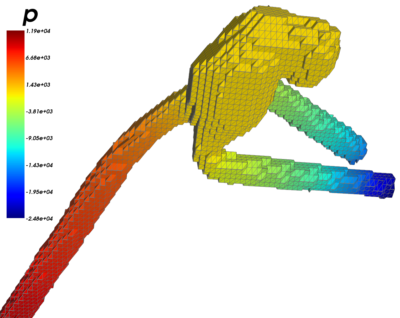
Fig. 8.4: Stokes flow in an aneurysm. Top: Aneurysm surface embedded in the structured background mesh $\widehat{\mathcal{T}}^{\ast}$. Bottom: Fictitious domain $\Omega^{\ast}$ and corresponding mesh $\mathcal{T}^{\ast}$ with pressure approximation.

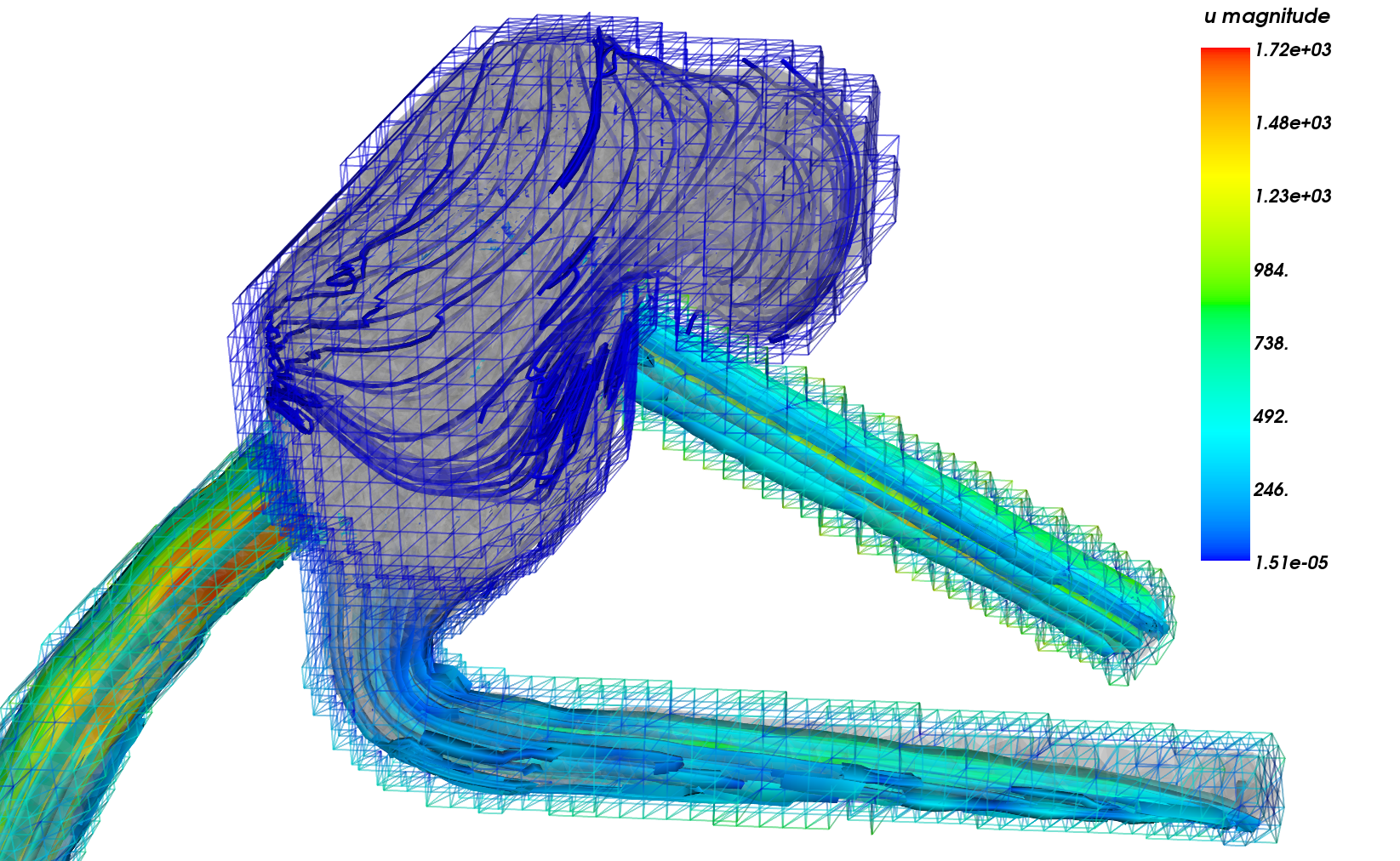
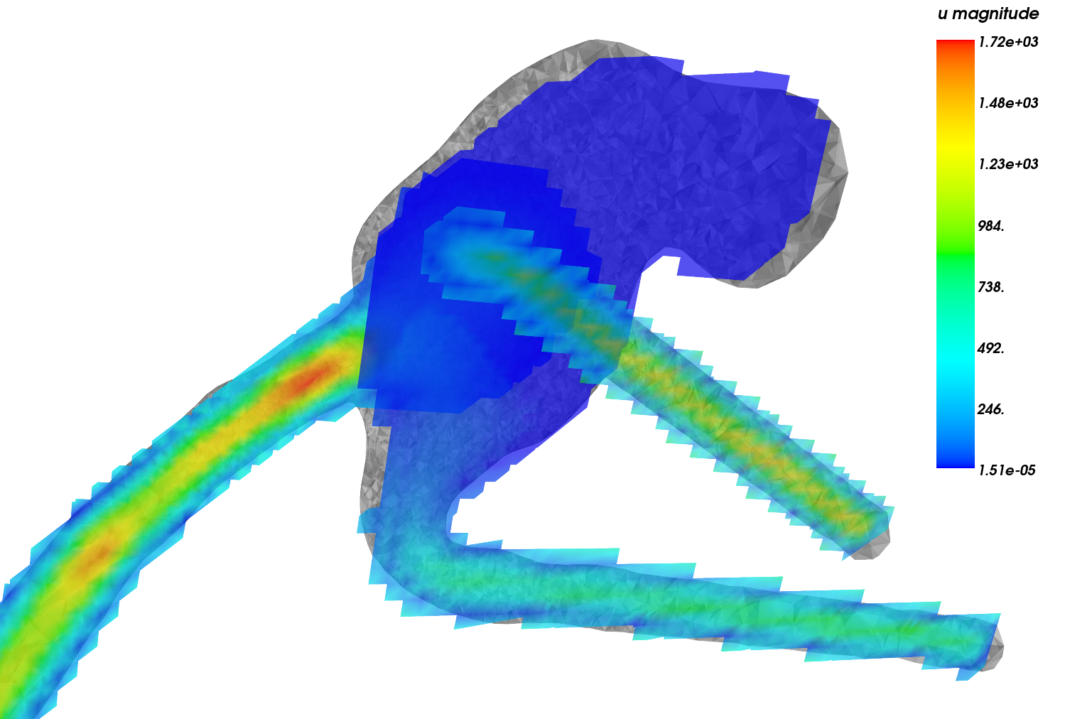
Fig. 8.5: Velocity approximation on $\mathcal{T}^{\ast}$. Top: Original aneurysm embedded in the background mesh shown with velocity streamlines. Bottom: Three cross-section through the aneurysm showing the magnitude of the velocity in each vessel section. Despite the coarse approximation of the aneurysm geometry by the fictitious domain mesh, the boundary values of the velocity respect the underlying surface geometry.

9 Conclusions

We have presented a stabilized finite element method for the solution of the Stokes problem on fictitious domains and proved optimal order convergence. The theoretical convergence rates have been verified numerically. We have also proved that the condition number of the stiffness matrix remains bounded, independently of the position of the fictitious boundary relative to the background mesh.

While we have here restricted our attention to the static Stokes model problem, the main motivation for the methodology and implementation presented in this paper is for the treatment of the time-dependent Navier–Stokes equations and, ultimately, fluid–structure interaction on complex and evolving geometries. We address this issue in future work.

References

- [1] Cgal, Computational Geometry Algorithms Library, software package. URL http://www.cgal.org.
- [2] gts, GNU Triangulated Surface Library, software package. URL http://gts.sourceforge.net/.
- Alnæs [2012] Martin S. Alnæs. UFL: a Finite Element Form Language, chapter 17. Springer, 2012.
- Alnæs et al. [2012] Martin S. Alnæs, Anders Logg, and Kent-Andre Mardal. UFC: a Finite Element Code Generation Interface, chapter 16. Springer, 2012.
- Barth et al. [2004] Teri Barth, Pavel Bochev, Max Gunzburger, and John Shadid. A Taxonomy of Consistently Stabilized Finite Element Methods for the Stokes Problem. SIAM J. Num. Anal., 25(5):1585, 2004.
- Becker et al. [2009] Roland Becker, Erik Burman, and Peter Hansbo. A Nitsche extended finite element method for incompressible elasticity with discontinuous modulus of elasticity. Comput. Methods Appl. Mech. Engrg., 198(41-44):3352–3360, 2009.
- Bochev et al. [2006] P.B. Bochev, C.R. Dohrmann, and M.D. Gunzburger. Stabilization of low-order mixed finite elements for the Stokes equations. SIAM J. Num. Anal., 44(1):82, 2006.
- Brenner and Scott [2008] Susanne C. Brenner and L. Ridgway Scott. The mathematical theory of finite element methods, volume 15 of Texts in Applied Mathematics. Springer, New York, third edition, 2008.
- Brezzi and Fortin [1991] Franco Brezzi and Michel Fortin. Mixed and hybrid finite element methods, volume 15 of Springer Series in Computational Mathematics. Springer-Verlag, New York, 1991.
- Burman [2010] E. Burman. Ghost penalty. Comptes Rendus Mathematique, 348(21-22):1217–1220, 2010.
- Burman and Hansbo [2012a] E. Burman and P. Hansbo. Fictitious domain finite element methods using cut elements: II. A stabilized Nitsche method. Appl. Numer. Math., 62(4), 2012a.
- Burman and Hansbo [2012b] Erik Burman and Peter Hansbo. Fictitious domain methods using cut elements: III. A stabilized nitsche method for stokes’ problem. Technical Report 2011:06, School of Engineering, Jönköping University, JTH, Mechanical Engineering, 2012b.
- Ern and Guermond [2006] A. Ern and J.L. Guermond. Evaluation of the condition number in linear systems arising in finite element approximations. ESAIM, Math. Model. Num. Anal., 40(1):29–48, 2006.
- Franca et al. [1993] L.P. Franca, T.J.R. Hughes, and R. Stenberg. Stabilized finite element methods for the Stokes problem. In M.D. Gunzburger and R. A. Nicolaides, editors, Incompressible Computational Fluid Dynamics. Cambridge University Press, 1993.
- Girault et al. [2005] V. Girault, B. Rivière, and M. F. Wheeler. A discontinuous Galerkin method with nonoverlapping domain decomposition for the Stokes and Navier-Stokes problems. Math. Comp., 74(249):53–84, 2005.
- Glowinski and Kuznetsov [2007] R. Glowinski and Y. Kuznetsov. Distributed Lagrange multipliers based on fictitious domain method for second order elliptic problems. Comput. Methods Appl. Mech. Engrg., 196(8):1498–1506, 2007.
- Glowinski et al. [2001] R. Glowinski, T. W. Pan, T. I. Hesla, D. D. Joseph, and J. Périaux. A Fictitious Domain Approach to the Direct Numerical Simulation of Incompressible Viscous Flow past Moving Rigid Bodies: Application to Particulate Flow. Journal of Computational Physics, 169(2):363–426, 2001.
- Hansbo and Hansbo [2002] A. Hansbo and P. Hansbo. An unfitted finite element method, based on Nitsche’s method, for elliptic interface problems. Comput. Methods Appl. Mech. Engrg., 191(47-48):5537–5552, 2002.
- Hughes et al. [1986] Thomas J. R. Hughes, Leopoldo P. Franca, and Marc Balestra. A new finite element formulation for computational fluid dynamics. V. Circumventing the Babuška-Brezzi condition: a stable Petrov-Galerkin formulation of the Stokes problem accommodating equal-order interpolations. Comput. Methods Appl. Mech. Engrg., 59(1):85–99, 1986.
- Hughes et al. [1989] T.J.R. Hughes, L.P. Franca, and G.M. Hulbert. A new finite element formulation for computational fluid dynamics: VIII. The Galerkin/least-squares method for advective-diffusive equations. Comput. Methods Appl. Mech. Engrg., 73(2):173–189, 1989.
- Isaksen et al. [2008] J. G. Isaksen, Y. Bazilevs, T. Kvamsdal, Y. Zhang, J. H. Kaspersen, K. Waterloo, B. Romner, and T. Ingebrigtsen. Determination of wall tension in cerebral artery aneurysms by numerical simulation. Stroke, 39(12):3172, 2008.
- Johansson and Larson [2012] August Johansson and Mats G. Larson. A high order discontinuous Galerkin Nitsche method for elliptic problems with fictitious boundary. submitted to Numerische Mathematik, 2012.
- Kechkar and Silvester [1992] Nasserdine Kechkar and David Silvester. Analysis of Locally Stabilized Mixed Finite Element Methods for the Stokes Problem. Math. Comp., 58(197):1, January 1992.
- Kirby and Logg [2006] Robert C. Kirby and Anders Logg. A Compiler for Variational Forms. ACM Trans. Math. Softw., 32(3):417–444, 2006.
- Logg [2007] Anders Logg. Automating the finite element method. Arch. Comput. Methods Eng., 14(2):93–138, 2007.
- Logg and Wells [2010] Anders Logg and Garth N. Wells. DOLFIN: Automated finite element computing. ACM Trans. Math. Softw., 37(2), 2010.
- Logg et al. [2012a] Anders Logg, Kent-Andre Mardal, Garth N. Wells, et al. Automated Solution of Differential Equations by the Finite Element Method. Springer, 2012a.
- Logg et al. [2012b] Anders Logg, Kristian B. Ølgaard, Marie E. Rognes, and Garth N. Wells. FFC: the FEniCS Form Compiler, chapter 11. Springer, 2012b.
- Massing et al. [2012a] A. Massing, Mats G. Larson, and A. Logg. Efficient implementation of finite element methods on non-matching and overlapping meshes in 3D. submitted, 2012a.
- Massing et al. [2012b] A. Massing, Mats G. Larson, A. Logg, and Marie E. Rognes. A stabilized Nitsche overlapping mesh method for the Stokes problem. submitted, 2012b.
- Quarteroni [2009] Alfio Quarteroni. Numerical Models for Differential Problems. Modeling, Simulation and Applications. Springer-Verlag, 2009.
- Scott and Zhang [1990] R. Scott and S. Zhang. Finite element interpolation of nonsmooth functions satisfying boundary conditions. Math. Comp., 54(190):483–493, 1990.
- Stein [1970] E. Stein. Singular Integrals and Differentiability Properties of Functions. Princeton University Press, 1970.
- Steinman et al. [2003] D. A. Steinman, J. S. Milner, C. J. Norley, S. P. Lownie, and D. W. Holdsworth. Image-based computational simulation of flow dynamics in a giant intracranial aneurysm. AJNR. American journal of neuroradiology, 24(4):559–66, April 2003.
- Valen-Sendstad et al. [2011] Kristian Valen-Sendstad, Kent-André Mardal, Mikael Mortensen, Bjørn Anders Pettersson Reif, and Hans Petter Langtangen. Direct numerical simulation of transitional flow in a patient-specific intracranial aneurysm. Journal of biomechanics, 44(16):2826–32, November 2011.
- Verfürth [1994] R. Verfürth. A posteriori error estimation and adaptive mesh-refinement techniques. In Proceedings of the fifth international conference on Computational and applied mathematics table of contents, pages 67–83. Elsevier Science Publishers BV Amsterdam, The Netherlands, The Netherlands, 1994.
- Yu [2005] Z. Yu. A DLM/FD method for fluid/flexible-body interactions. Journal of Computational Physics, 207(1):1–27, 2005.