Non-perturbative features of driven scattering systems

Abstract

We investigate the scattering properties of one-dimensional, periodically and non-periodically forced oscillators. The pattern of singularities of the scattering function, in the periodic case, shows a characteristic hierarchical structure where the number $N_{c}$ of zeros of the solutions plays the role of an order parameter marking the level of the observed self-similar structure. The behavior is understood both in terms of the return map and of the intersections pattern of the invariant manifolds of the outermost fixed points. In the non-periodic case the scattering function does not provide a complete development of the hierarchical structure. The singularities pattern of the outgoing energy as a function of the driver amplitude is connected to the arrangement of gaps in the fundamental regions. The survival probability distribution of temporarily bound orbits is shown to decay asymptotically as a power law. The ”stickiness” of regular regions of phase space, given by KAM surfaces and remnant of KAM curves, is responsible for this observation.

I Introduction

In a scattering problem the system is characterized by having a localized region of configuration space (’interaction region’) where the interaction is relevant, while elsewhere the interaction is absent. A particle is injected into the interaction region and experiences a scattering event; after each event it may escape from the interaction region forever (’scattered’ trajectories) or eventually proceed to another scattering event. A map that links some initial parameter to some feature of the outgoing state is called a scattering function. There may exist ’trapped’ trajectories, i.e. particles that wander for ever in the interaction region. In these circumstances the scattering function is not defined. A scattering process is called ’irregular’ or ’chaotic’ when a scattering function is singular on a fractal set of variable initial values (see Ref. Eckhardt-1988, ).

A condition for having chaotic scattering is the existence of an invariant set $\Lambda$ of an infinite number of unstable, periodic and aperiodic orbits, localized in the interaction region. Whenever $\Lambda$ contains a Cantor set, irregular scattering occurs. In fact the stable manifolds of orbits in $\Lambda$ reach out into the asymptotic region by means of the Hamiltonian flow; an orbit started on one of the stable manifolds is captured in the interaction region for all the time, i.e. the final state is not defined. Hence there exists a fractal set of asymptotic in-variables (the initial conditions lie in the stable manifolds of orbits in $\Lambda$) where the scattering function is singular JS-1987 ; JS-1988 . The pattern of homoclinic/heteroclinc connections of invariant manifolds of $\Lambda$ is called ’chaotic saddle’.

Therefore incoming parameters close to each other and close to the ’stable manifold’ of the chaotic saddle can be mapped to very different outgoing parameters. They spend a long time in the vicinity of $\Lambda$  and trace out the type of motion performed by the localized trajectories. Similarly outgoing parameters close to each other and close to the unstable manifold can come from very different incoming parameters. $\Lambda$ acts as a ”repeller” with global influence on the asymptotic region. Therefore the scattering function displays wild fluctuations on all scales on each set containing initial conditions leading to trapped orbits. The origin of the fractal singularities of a scattering function is the chaotic motion in the invariant bound set; the irregularity of the motion in an unbound phase space is connected to a form of bound chaos.

Thus, the main issue in studying a problem of chaotic scattering is to determine the properties of the invariant set, in particular the topological pattern of the chaotic saddle and the character of the dynamics in it. In this regard it is hoped that an equivalent symbolic dynamics is found out to explain the behavior of a scattering function. The invariant set provides a fractal structure whose dimension, Lyapunov exponents and escape rate can be connected to the particular arrangement of the singularities in the scattering function or in the delay time function.

The chaotic (invariant) set shows a relatively simple structure when it is completely hyperbolic. In this case it consists of unstable periodic orbits (all of them are hyperbolic) and their homoclinic and heteroclinic connections only. As Smale shows smale-1967 , this is connected with the horseshoe construction. A system with $n$ fixed points (periodic solutions) corresponds to a horseshoe with the same number of fixed points; one can obtain the horseshoe structure by plotting the invariant manifolds of any unstable periodic point. The invariant set may contain KAM tori and sets of marginal stability; in this case it is not completely hyperbolic and the horseshoe is not fully developed. We will present a system which differs from a standard Smale’s horseshoe model:

• the configuration space is infinite, the interaction is long ranged and parabolic orbits exist; it follows that the invariant set is not compact and the system is described by a symbolic dynamics with an infinite number of symbols;

• in the phase space there are islands which consist of unbroken KAM surfaces.

Many physical scattering systems can be modeled in the following way. We consider a set $S$ in the phase space. A driving force removes a fraction of points from $S$ after each step of an iterative process: after the first step, it leaves a number of intervals in $S$, after the second step a set of new subintervals replaces each old interval. This process can be infinitely repeated. The structure of the set of points that are never removed is Cantor-like. This process is characteristic of systems with fully developed chaos.

In chaotic scattering the Smale’s mechanism leads to an exponential decay of phase space ensembles: all phase space points are depleted except for the invariant set, which consists of all trapped orbits of the system. However the assignment of an exponential decay law to a chaotic dynamics is not general. When in the phase space some regular islands with KAM surfaces survive, the particle initialized in a chaotic region can spend a long time near the boundary of a regular region. In this case, the leaving away of the particles from the KAM region gives an algebraic decay Chirikov-Shepelyanski ; Karney ; Meiss-Ott .

The existence of KAM surfaces is not the only mechanism resulting in an algebraic decay. In the Ref. Hillermeier-Blumel-Smilansky, the authors present a chaotic system that does not show any KAM structures and that decays according to a power law. The scaling is explained through a model of random walk in phase space; the dynamics of symbolic strings is Markovian. Beeker et al. Beeker-Eckelt observe an algebraic scaling of the scattering function. Nevertheless they claim that the KAM component effects are negligible for the parameter values they choose. Beeker et al. provide reasons for the scaling by means of a different mechanism than the stickiness of KAM tori. They consider the survival time of the temporarily bound orbits close to the parabolic orbit. If the system is described by a symbolic dynamics with infinite symbols, one can have a chaotic dynamics in a phase space without any regular region and, at the same time, a scaling with a power law.

When an external control parameter is varied, the invariant set changes its structure. In particular, if some non-hyperbolic components enlarge, then the stable and unstable bundles can be displaced one with respect to each other. For certain parameter values, intersections are destroyed and some localized orbits of the invariant set get lost, i.e. bifurcations take place. As a consequence, the invariant set may be no longer topologically equivalent to a complete Cantor set. Some relevant quantities (such as the escape rate and the topological entropy) have general features: as functions of the parameter they display plateaux, where no orbits disappear. There is also a set of parameter values where the quantities change indicating the presence of bifurcations. This set can have an involved structure; in fact for a class of systems the topological entropy exhibits a devil’s staircase Lai-Zyczkowski-Grebogi .

There is a wide variety of applications of the chaotic scattering in classical physics.

In celestial mechanics complicated motions can take place for close encounters, but, after, the particles separate, with the exception of a set of initial conditions of zero measure Petit-Henon .

In many chemical reactions (in particular, in the case of a biatomic molecule interacting with an atom) small changes in the initial conditions lead to drastic differences in the final states so that a nonreactive trajectory may exist in the vicinity of a reactive one. Pollack et al. Pechukas emphasized the importance of unstable periodic orbits that, typically, provide a non-attracting, infinite set Koch-Bruhn . Skodje et al. Skodje got a chaotic scattering approach to the matter.

In hydrodynamics the scattering among more than three ideal, linear vortices can bring to chaotic dynamics. Aref and Eckhardt et al. Eckhardt-Aref ; Aref draw attention to the processes occurring in the interaction. Two couples of vortices that interact can either pass by each other or exchange their partners and then spend time moving along circular motion, until the next collision when they can either convert to the original couples or scatter away from each other. This capture state is unstable and exhibits all properties of chaotic scattering, and, in particular, it may be disrupted by a small change in the parameters.

There are many applications of the chaotic scattering to the classical scattering problem by a potential. The heart of all examples is the existence of unstable, bounded orbits that trap a set of orbits in the continuum of the scattering trajectories and lead to singularities in the scattering functions EJ-1986 ; Jung-1986 ; Jung-1987 ; JS-1987 . A particular class of problems is connected with the internal dynamics of atomic systems or clusters interacting with an external electromagnetic field. Even if the motion is integrable in the field-free case, external driving generically destroys integrability and can lead to irregular dynamics, sensitive with respect to both initial conditions and parameters of the driver. This class of systems contains models of one-dimensional oscillating potential wells.

In this paper we deal with a representative of this class of systems: the model of ’rigid spheres’ Mulser ; Kundu-Bauer . It is introduced in connection with the problem of the energy absorption in clusters irradiated by intense electromagnetic fields; the model provides a basic mechanism of absorption. We focus on some features of the dynamics of the model. These features are understandable by means of a chaotic scattering approach.

In section 2, we introduce the model and we list the particular cases we consider in the numerical study. In section 3, we summarize the relevant numerical results about the scattering function and its structure of singularities; the geometry of the scattering function is dominated by the escape orbits while the singularities are caused by the captured orbits. We show that the scaling of the delay time function is algebraic. In section 4, following Alekseev alekseev ; alekseev-3 and Ref. Eckelt-Zienicke, we introduce a return map and we obtain a detailed description of the structure of the scattering function. In section 5, we give a different approach to the investigation of the structure of the scattering function. We construct the pattern of intersections of invariant manifolds of the two outermost fixed points. The singularities structure of the delay time function corresponds to the pattern in which the bundles of stable manifolds intersect the local segment of the unstable manifold. As Smale has shown, the homoclinic/heteroclinic bundle is connected with a horseshoe construction. We obtain that the horseshoe map is not completely developed due to the non-hyperbolic effects created by the surfaces of KAM islands and their secondary structures; they cause the algebraic behavior in the statistics of the delay time function. In section 6, we investigate the outgoing energy as a function of the driver amplitude for fixed initial conditions. We observe that this function displays behaviors similar to the scattering function. This is interpreted through some essential properties of the topology of the homoclinic/heteroclinic bundle. The discrepancies between the two functions depend on secondary aspects of the topology.

II The problem

We study the scattering of a particle (mass m=1) by a one-dimensional potential well $V(x)$, $x\in\mathbb{R}$, driven by a homogeneous, time dependent force $f$.

The potential we consider is attractive, bell-shaped, symmetric, limited, with a single equilibrium point. The definite expression we treat is provided by the model of rigid spheres. It is a simple electrostatic system where a negatively charged sphere moves in the potential generated by a fixed, positively charged one. The potential is Coulomb-like when the spheres do not overpose; otherwise it is polynomial. Following Ref. Kundu-Bauer, we assume

$$V_{1}(x)\ =\left\{\begin{array}[]{lc}1/2\,x^{2}\,-\,3/16\,|x|^{3}\,+\,1/160\,|x|^{5}&|x|\leq 2\\ -1/|x|\,+\,6/5&otherwise\end{array}\right.$$ (1)

$V_{1}$ is $\mathbb{C}^{2}$ for $x\in\mathbb{R}$.

For reference, we also perform simulations with a Lorentz-shaped potential $V_{2}$ characterized by general features similar to $V_{1}$ except for being $\mathbb{C}^{\infty}$.

$$V_{2}(x)\ =\ \frac{6/5\ x^{2}}{(12/5\,+\,x^{2})}$$ (2)

We also test potentials of different shapes with the same general features: the results relevant for our discussion are essentially the same.

The system is driven by a homogeneous, time-dependent force $f$ representing the effect of an applied oscillating electric field. We study two cases: $f=f_{1}$ (compact support) and $f=f_{2}$ (periodic).

$$f_{1}(t)\ =\,\left\{\begin{array}[]{lc}e_{0}\sin^{2}(\frac{\nu\,t}{n})\ \,\cos(\nu\,t)&0\leq\nu\,t\leq n\,\pi\\ 0&otherwise\end{array}\right.$$ (3)

$n$ in $\mathbb{N^{+}}$  $n>>1$. The support of the envelope is one period of $\sin^{2}(\frac{\nu\,t}{n})$; in this way it is introduced a time scale $n/\nu$ . Therefore $f_{1}$ is defined by the amplitude $e_{0}$, the width of the envelope and the frequency $\nu$ of the co-sinusoidal factor.
The second form of $f$ we study is purely sinusoidal

$$f_{2}(t)=e_{0}\sin(\nu\,t)$$ (4)

We always assume $\nu>1$.

The time-dependent Hamiltonian is given by

$$\begin{split}H(p,\,x,\,t)&=\,H_{0}(p,\,x)\ -\ e_{0}\ f(t)\ x\\ &=\ p^{2}/2\ +\ U(x,\,t)\end{split}$$ (5)

where $H_{0}(p,\ x)=\,p^{2}/2\ +\,\omega^{2}\ V(x)$, and, according to the case, $V=V_{i}$ and $f=f_{i}$ , $i=1,2$. In both cases the undriven oscillators are characterized by a linear angular velocity $\omega=0.7$ and an escape solution $x_{h}$ (’heteroclinic’ orbit) with parabolic critical points, i.e. $|x_{h}(\pm\infty)|=\infty$ and $\dot{x}_{h}(\pm\infty)=0$. The energy of the unperturbed escape orbit is $6/5\,\omega^{2}=0.588$ .

The phenomenology we study concerns drivers with strength even many times the maximal oscillator force. Therefore it cannot be fully understood only through perturbative methods. However there are some perturbative treatments (in particular Moser-73 ; Cicogna-01 ; Dankowicz ) that show the important role of the escape orbit in the explanation of the irregular dynamics of the driven oscillators. Thus we concentrate on orbits in the phase space with energies not far from the escape energy of the free oscillator. In such situations, at fixed strength of the driver, in the phase space there are size-able regions of initial conditions characterized by unstable trajectories which appear to be so erratic that the system motions can be regarded as stochastic. Elsewhere, irregular motions are absent. In addition, if the strength of the driver is varied then stochastic regions move in the phase space.

The properties of the dynamics can be approached by studying the scattering functions, i.e. maps connecting the initial states to the final ones, after a time long enough such that the particle can move in the interaction region and possibly comes out of it. In order to determine the scattering functions, we are interested in asymptotic data. For the case $f=f_{1}$ we get the relevant quantities at $t\geq n\,\pi/\nu$. The driver should play the role of a transient. Actually, we find that the main descriptive properties are developed, at least partially, before the end of the transient. In the case $f=f_{2}$ we simply take the data after many periods of $f_{2}$.

The maps we obtain display the irregular behavior of the dynamics: intervals of the initial state variables, where the map is sensitively depending on, alternate with intervals where the map is smooth.

The irregular behavior of the scattering functions can be analyzed through the approach of the irregular scattering theory. Actually the chaotic scattering theory deals with physical situations where the dynamics takes place in an infinite volume of the phase space, the interaction is confined to a finite region and there are some scattering functions which display wild fluctuations on all scales.

We briefly give an outline of the main results of the numerical calculations.

• For both the oscillators with the sinusoidal driver $f_{2}$ we determine two scattering functions. For a trajectory with initial velocity $\mathrm{v}_{0}$ we get the energy $H_{0}$ and the number $N_{c}$ of crossings through $x=0$ after the particle has moved out from the interaction region.
  Then we plot $H_{0}$ and $N_{c}$ as functions of $\mathrm{v}_{0}$. Both of the maps display the same sequence of intervals of $\mathrm{v}_{0}$ where the outgoing variable ($H_{0}$ or $N_{c}$) is smooth. Between these intervals there are gaps in which $H_{0}$ and $N_{c}$ jump in an irregular way. Hence there is a correspondence between the number of crossings through the origin and the regular intervals for $H_{0}$.

• An analogous analysis is performed with the driver $f_{1}$. The patterns of the scattering functions are qualitatively similar to the previous ones.

• We initialize at $t=0$ an ensemble of scattering orbits and we calculate the number $N(t)$ of orbits that are still inside the interaction region at the time $t$. We obtain an algebraic decay law.

• For the same ensemble the distribution of zeros $N(n)$ is determined. For the considered parameters of the simulation we again obtain a power law.

• We fix the initial conditions and we calculate $H_{0}$ and $N_{c}$ as functions of the parameter $e_{0}$. The resultant plots show the same structures described for the previous scattering functions

Note

A resonance may be a rich source of highly complex motions (see Ref. Haller1999, ), as chaotic patterns and irreversibility in the transfer of energy between different oscillatory states. It takes place only if the system stays in one of those particular regions of the phase space in which the frequencies of some angular variables become nearly commensurate. We guess that the irregular motions of the systems we consider are due to a mechanism distinct from and more general than a resonance. Actually we avoid the resonance condition, since the driver frequency $\nu$ is larger than the highest ’effective’ frequency of the free oscillator.

III Numerical results.

We use the Runge-Kutta algorithm of fourth order to integrate the Hamilton’s equations (5). In order to check our code, we solve the rigid spheres model and we compare with the same simulations in Ref. Kundu-Bauer, .

III.1 Scattering functions

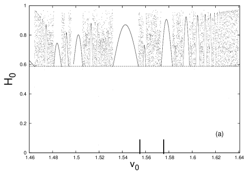
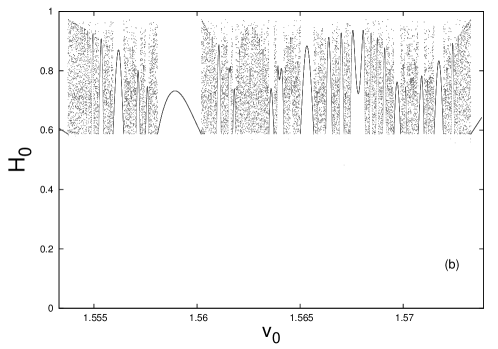
Figure 1: The map of the outgoing energy $H_{0}$ vs the initial velocity $\mathrm{v}_{0}$ for $x(0)=0$ with $e_{0}=1$ and $\nu=0.8$. Plot $(b)$ is a magnification of the marked interval of plot $(a)$.

A scatterig function is a map connecting some variables that refer to states before the interaction to some other concerning states after it. Our choice of the variables of the mapping is partially different from that in Refs. Beeker-Eckelt, and Eckelt-Zienicke, .

When $f=f_{1}$  we obtain the map

$$S^{1}_{(x_{0},e_{0})}:\ \ (x(0)=0,\ \mathrm{v}(0)=\mathrm{v}_{0})\ \,\mapsto\ \,H_{0}(p(t^{\ast}),\,x(t^{\ast}))$$

$t^{\ast}>\,n\,\pi/\nu$ , $n=340$, i.e. it links the initial conditions ($0$, $\mathrm{v}_{0}$) of a trajectory to the energy $H_{0}$ of the trajectory at a time $t^{\ast}$ after the driver $f_{1}$ is switched off. The driver amplitude $e_{0}$ is treated as a parameter. Analogous maps are obtained as functions of $x_{0}$ for a given $\mathrm{v}_{0}$. When $f=f_{2}$ (periodic case) we consider the map

$$S^{2}_{(x_{0},e_{0})}:\ \ (x(0)=0,\ \mathrm{v}(0)=\mathrm{v}_{0})\ \,\mapsto\ \,H_{0}(p(t_{k}),\,x(t_{k}))$$

$\nu\,t_{k}\ =\,2\,k\,\pi$ , $k=1,\ 2\,,\ \ldots$. It is a map from one value to many ones which connects the initial conditions ($0$, $\mathrm{v}_{0}$) to the energies $H_{0}$’s taken at times $t_{k}$ such that $t_{k+1}-t_{k}$ is one driver period.

In all the cases the dependence of $H_{0}$ on $\mathrm{v}_{0}$ alternates between regular intervals, where $S^{i}_{(x_{0},e_{0})}$ , $i=1,\,2$, shows a smooth behavior, and irregular intervals, where $S^{i}_{(x_{0},e_{0})}$ is much more sensitive. In the plot $(a)$ of fig. 1 we present the results for the $\mathrm{v}_{0}$ interval $[1.46,\,1.64]$. Plot $(b)$ of fig. 1 is an expansion of the irregular interval marked in the plot (a) ($\mathrm{v}_{0}$ varies in $[1.5533:1.5739]$).

Figure 2: The number of zeros $N_{c}$ of a trajectory with initial velocity $\mathrm{v}_{0}$ ($x(0)=0$); the marked interval of $(a)$ is magnified in $(b)$; the plot $(c)$ shows a sequence of intervals with three zeros that accumulates to a two zeros interval as $\mathrm{v}_{0}$ approaches the border of the two zeros interval.

An orbit may be marked by the number $N_{c}$, the number of crossings of $x=0$. Another scattering map we obtain is $N_{c}$ as a function of $\mathrm{v}_{0}$; it is displayed in the part $(a)$ of fig. 2. We note the following features:

• $N_{c}$ is constant in each interval where the scattering map is regular; $N_{c}$ and the scattering map are singular at the same points (compare (a) of fig. 1 to (a) of fig. 2);

• each regular interval between two regular ones with the same $N_{c}$ has a crossing number greater than $N_{c}$;

• in the region between two regular intervals with the same $N_{c}$, a sequence of $N_{c}+1$ regular intervals accumulates as $\mathrm{v}_{0}$ gets next to the boundaries of the region (see (b) and (c) of fig. 2).

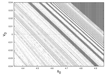
Figure 3: Distribution of initial conditions of nearest trajectories with the same number of crossings of the origin. We choose an ensemble of orbits with an uniform distribution of initial conditions and we mark an initial condition whenever its orbit experiences the same $N_{c}$ as the orbits from the closest initial conditions.

• 

Figure 4: The plot shows $N_{c}$ versus the initial conditions in the same numerical experiment as in fig. 3. Note the stripes arrangement of the structure and the hierarchy of stripes according to what described above. The $N_{c}$ stripes accumulate going close to a $N_{c}-1$ stripe.

Figure 5: There are shown some details of fig. 4. In $(a)$ there is a sequence of stripes $N_{c}=2$ approaching the domain $N_{c}=1$. $(b)$ is an example of the structure with a sequence of $N_{c}+1$ stripes accumulating against a $N_{c}$ domain.

These rules define the ’hierarchy’ of the structure of the scattering function and of the delay time function.

A trajectory belonging to a regular interval spends a finite time in the interaction region since, we know, it experiences a finite number of zeros. When the trajectory leaves out the interaction region, only the driver has an effect on the particle and therefore the values of $H_{0}$ at times $t_{k}$, taken at the end of each driver period (see the definition of $S^{2}_{x_{0},\,e_{0}}$), are almost constant, i.e. for $\mathrm{v}_{0}$ in a regular interval the map $S^{2}_{x_{0},\,e_{0}}$ is characterized by a ’fixed’ point (see fig. 1).

The horizontal line in fig. 1 - $(a)$ displays the energy $h^{\prime}$ of the unperturbed escape orbit ($0.588$ in our cases). From the plot we may state that if $\mathrm{v}_{0}$ is in a regular interval then $H_{0}\geq h^{\prime}$ for all times large enough. An orbit belonging to a regular region is called hyperbolic and parabolic when $H_{0}>h^{\prime}$ and $H_{0}=h^{\prime}$, respectively.

We note that a magnification of an irregular interval between two regular intervals with $N_{c}$ zeros gives a pattern qualitatively similar to the complete one; the irregular gap in $(a)$ dissolves into a sequence of regular subintervals, with at least $N_{c}+1$ zeros, separated by irregular gaps. Whenever we continue in this way we find an intertwined structure of regular and irregular intervals; at each step the distribution of regular intervals, marked by the number of zeros, meets the three rules listed above.

From our numerical inspection we are driven to argue that $S^{2}_{(x_{0},\,e_{0})}$ should possess fractal features; the scattering function is continuous for all $\mathrm{v}_{0}$ except a set $\mathcal{C}$ of singularities. $\mathcal{C}$ is the set of points after removing all the regular intervals with any number $N_{c}$ of zeros. We guess the measure of $\mathcal{C}$ should be zero. In fact $\mathcal{C}$ appears to be determined in analogy to the hierarchical procedure of a Cantor set, by giving level by level the endpoints of cut out intervals.

Fig. 3 illustrates the distribution of the nearest trajectories which cross the origin the same number of times. Starting from a uniformly distributed ensemble of initial conditions, we mark a pair $(x_{0},\,\mathrm{v}_{0})$ of initial conditions only if its trajectory experiences the same number of zeros as the trajectories corresponding to the closest pairs. The plot shows a pattern organized as a sequence of stripes accumulating to a domain corresponding to parabolic and hyperbolic orbits with only one zero, i.e. to the set of initial conditions of orbits that escape after crossing once the origin. Each stripe in the figure is marked by a determined $N_{c}$.

Fig. 4 displays the distribution of the number of zeros $N_{c}$, with $1\leq N_{c}\leq 6$, extracted from the fig. 3. We observe the hierarchical structure, ordered with respect to $N_{c}$ and described above. In particular we point out that the pattern is arranged in sequences of stripes that accumulate at the border of the domain with $N_{c}=1$ (see $(a)$ in fig. 5). In the hierarchy of the structure the level $N_{c}+1$ is a sequence of stripes approaching the stripe $N_{c}$ (see $(b)$ in fig. 5) as well.

A similar hierarchy is observed by Eckelt at al. Eckelt-Zienicke for a class of oscillators characterized by attractive potentials. In order to explain the properties of the hierarchy, they use a map (return map) introduced by Alekseev alekseev . We guess that the mechanism acting in our problem should be treatable in the same way by a suitable return map: we will come back to it in the next section.

• 

Figure 6: Scattering map and $N_{c}$ function of the oscillator (2) with the driver (3). Plot $(b)$ is an enlargement of the marked interval in $(a)$. Plot $(d)$ is a magnification of the marked interval in $(c)$. We note that the hierarchical structure is not fully developed.

We also consider the non periodic case ($f=f_{1}$) and compute the map $S^{1}_{(x_{0},\,e_{0})}$ that is calculated when the driver is already switched off and the energy $H_{0}$ is constant. The plots in $(a)-(d)$ of fig. 6 display the results; we set $e_{0}=1$ and we choose $\nu=1$ and $n=360$ in (3). As above an orbit for $\mathrm{v}_{0}$ in a regular interval is called hyperbolic and parabolic when $H_{0}>h^{\prime}$ and $H_{0}=h^{\prime}$ respectively.
$S^{1}_{(x_{0},\,e_{0})}$ displays structures that seem qualitatively similar to $S^{2}_{(x_{0},\,e_{0})}$; but note that the hierarchical structure does hold only partially. Between two $N_{c}$ intervals there are no intervals with a number of crossings less than $N_{c}$. However some sets of orbits result to be lost: in particular they are orbits in the vicinity of parabolically escaping ones (see $N_{c}\geq 3$ orbits in $(d)$ of fig. 6). These orbits have a very long return time and the number of their $x=0$ crossings depends on the duration of the driver in a more considerable way. This result is expected. A driver of infinite duration is needed so that the map structure can display a complete hierarchical pattern; a fractal generating mechanism needs an infinite iterative process.

III.2 The delay time function and scaling properties.

We now focus on the relation between the time of permanence in the interaction region and the regularity of the motion. The time interval spent by the particle in the interaction region is called delay time.

Given an ensemble of orbits (initial conditions) we determine the ’survival function’ $N(t)$: it gives the number of orbits that have a delay time larger than $t$, i.e. the number of orbits that experience at least one crossing through $x=0$ at $t_{1}\geq t$. This definition is not exactly the same as that considered by some other authors Lai-Blumel-Ott-Grebogi-1992 ; Ding-Bountis-Ott ; Beeker-Eckelt and which needs a bound region around $x=0$ to be initially chosen and counts the number of orbits that still stay in the region at $t$.

In our case the set of initial conditions is defined by a uniform distribution of initial velocities in the interval $1.55\leq\mathrm{v}_{0}\leq 1.64$ and $x(0)=0$. The line of initial conditions intersects the stable manifolds of the invariant set transversally. A scaling law is extracted by plotting $N(t)$ vs $t$ in a log-log diagram shown in fig. 7. The plot is fitted by a straight line, i.e. $N(t)$ displays an algebraic behavior $N(t)\sim t^{z}$; the exponent is $z=1.60\pm 0.01$.

The power law in the long time tails of the delay time statistics is related to the non-hyperbolicity of the dynamics. We expect a behavior like $t^{-3/2}$ when KAM islands influence the scattering process (see Refs. Karney, , Chirikov-Shepelyanski, ) and $t^{-2}$ when parabolic surfaces influence the scattering process, but KAM islands do not.

• 

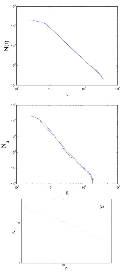
Figure 7: Log-log plots of $N(t)$ (plot $(a)$) and $N(n)$ (plot $(b)$) obtained from a sample of $2\ 10^{4}$ orbits whose initial velocity is uniformly chosen in (1.55, 1.57). Plot $(c)$ is an enlargement of the tail of the plot $(b)$ from the marked point; it shows a ’stair-case’ behavior of the distribution $N(n)$.

Another tool, that can be helpful to extract a statistical measure of the irregular dynamics in a scattering problem, is the distribution of the number of zeros. We consider the same ensemble of orbits as above; we determine the number $N(n)$ of orbits of the ensemble that perform at least $n$ crossings through $x=0$. We obtain again an algebraic law: $N(n)\sim n^{-z}$ for $z=2.33\pm 0.05$ (see fig. 7 - (b)). The power-law holds for $5\leq n\leq 60$. For $n>60$ $N(n)$ consists of a ’staircase’ structure (see fig. 7 - $(c)$) where the jumps take place at an irregular sequence of points. In Ref. Beeker-Eckelt,  it is obtained that $N(n)$ follows an exponential decay. The discrepancy is a consequence of a different choice of the parameters. We will come back to this point later.

IV The return map.

In this section we deal with a mapping that allows to reduce the analysis of the complete dynamical problem (5) to that of the states that either will still undergo at least a zero in the future or already underwent at least a zero in the past. Using this approach we can pick out an arrangement of the states that provides an explanation of the scattering map structure. In this section we deal with the periodic driver $f_{2}$.

The considered map, called return map, is introduced in the Refs. alekseev, and Eckelt-Zienicke, , where the authors investigate the irregular properties of the dynamics in periodically oscillating potential wells; they show that the map locally possesses the properties of the horseshoe. In our case we cannot conclude about the hyperbolicity of the invariant set because a better behavior of the potential $U(x,\,t)$, for $|x|\rightarrow+\infty$, is needed.

We define the return map $D$ on the Poincaré section $x=0$, that we denote by $\Gamma$. Consider a motion in which the particle crosses $x=0$ at the instant $t$, with momentum $p$. The conditions $(x=0,\,p,\,t)$  uniquely determine the solution $x(t^{\prime};\,p,\,t)$ of the problem (5). Whenever it exists consider the minimum time $t_{1}$, $t_{1}>t$, such that $x(t_{1};\,p,\,t)=0$. The return map is defined by

$$D\ :\ \ (p,\,t)\ \longrightarrow\ (p_{1},\,t_{1})$$ (6)

where $p_{1}$ is the momentum at $t_{1}$.

Note that

$$x(t^{\prime};\,p,\,t)\,=\,x(-t^{\prime};\,-p,\,t)\,=\,x(t^{\prime}\,+\,2\,\pi/\nu;\,p,\,t\,+\,2\,\pi/\nu)$$ (7)

since $H(p,\,x,\,t)=H(-p,\,x,\,-t)=H(p,\,x,\,\nu\,t\,+\,2\,\pi)$. It follows that the zeros of the solutions of problem (5) can be marked by the ’polar’ coordinates $p\geq 0$ and $\tau\equiv\nu\,t$. We denote by  $R^{+}\subset\Gamma$  the domain of $D$ (see fig. 8). Let us consider $(p,\,\tau)\in R^{+}$ and $(p^{\prime},\,\tau^{\prime})=D(p,\,\tau)$. There exists the maximum (whenever $x\geq 0$) or minimum (whenever $x\leq 0$) $X^{+}(p,\,\tau)$ of $x(t;\,p,\,\tau)$ in the interval $(\tau,\,\tau^{\prime})$.

In our case the energy is not conserved, but one can, all the same, define an energy-like function. For all $(p,\,\tau)$ in $R^{+}$ it is given

$$h^{+}(p,\,\tau)=\mathcal{V}(X^{+}(p,\,\tau))$$ (8)

where  $\mathcal{V}$ is the time average

$$\mathcal{V}(x)\,=\,1/(2\,\pi)\int_{0}^{2\,\pi}d\tau^{\prime}\ U(x,\,\tau^{\prime})$$

It is straightforward to show that $\mathcal{V}=V=V_{i}$, $i=1,\,2$. The function $h^{+}$ a composition of continuous applications; hence $h^{+}$ is a continuous function in $R^{+}$. We can extend by continuity the definition of $h^{+}$ at the boundary $P^{+}$ of $R^{+}$; $P^{+}$ consists of points $(\tilde{p},\,\tilde{\tau})$ such that if $(p,\,\tau)\in R^{+}$ approaches $(\tilde{p},\,\tilde{\tau})$ then $|X^{+}(p,\,\tau)|\rightarrow+\infty$ and

$$h^{+}(\tilde{p},\,\tilde{\tau})\,=\,\lim_{(p,\,\tau)\rightarrow\,(\tilde{p},\,\tilde{\tau})}h^{+}(p,\,\tau)\,=\,V(+\,\infty)$$

A point $(p,\,\tau)$ in the set $H^{+}=\Gamma\setminus(R^{+}\cup P^{+})$ is connected to an orbit $x(t;\,p,\,\tau)$ whose $X^{+}(p,\,\tau)$ is infinite; it follows that $\dot{x}(t;\,p,\,\tau)^{2}/2+V(x(t;\,p,\,\tau))\geq V(+\infty)$ for all $t$ large enough. The orbit $x(t;\,p,\,\tau)$ is called hyperbolic for $t\rightarrow+\infty$.

We may introduce analogous quantities following the solutions backwards in time. We focus on the set of all zeros $(p,\,\tau)\in\Gamma$ for which there exists $x(t^{\prime};\,p,\,\tau)=0$ at $t^{\prime}<\tau/\nu$, i.e. the particle returns to the origin if we follow the solution back to the past. We denote this set by $R^{-}$ (see fig. 8); it is the imagine of $R^{+}$ under the return map. If $(p,\,\tau)\in R^{-}$  then it exists a finite last turning point $X^{-}(p,\,\tau)$. The function $h^{-}(p,\,\tau)$ is defined in $R^{-}$, analogously to (8); now substitute $X^{-}$ for $X^{+}$. $h^{-}$ is continuous in $R^{-}$ and can be extended to the boundary $P^{-}$ of $R^{-}$. We introduce $H^{-}=\Gamma\setminus(R^{-}\cup P^{-})$, as well. The point $(p,\,\tau)$ is in $H^{-}$ whenever $X^{-}(p,\,\tau)$ is infinite; the solution $x(t,\,p,\,\tau)$ is called hyperbolic for $t\rightarrow\,-\infty$.

If $(p,\,\tau)$ is in $R^{+}$ then

$$\lim_{(p,\,\tau)\rightarrow P^{+}}t^{\prime}=+\infty$$ (9)

where $t^{\prime}$  is the time of the next following zero of the solution $x(t;\,p,\,\tau)$. Similarly,

$$\lim_{(p,\,\tau)\rightarrow P^{-}}t^{\prime\prime}=-\infty$$ (10)

where $t^{\prime\prime}$ is the time of the last previous zero of $x(t;\,p\,,\tau)$ for $(p,\,\tau)\in R^{-}$. The properties (9) and (10) will play an important role.

If $e_{0}=0$  $D=I$ and $h^{\pm}$ coincide with the energy integral ($h^{+}=h^{-}=H_{0}$). The set $R^{+}=R^{-}$ is the circle $|p|\leq(2\,V(\infty))^{1/2}$.

The return map is derived from the Hamiltonian system (5). The integral $\oint\omega$ of the Poincaré-Cartan invariant $\omega=p\,dx\,-\,H(p,\,x,,t)\,dt$ assumes the form $\oint_{c}(-p^{2}/2)\,d\tau$ on the section $\Gamma$, $c$ is the contour of a bounded area. It follows that $D$ is area preserving in $\Gamma$ ($p$ and $\tau$ are polar coordinate in $\Gamma$).

Whenever $e_{0}\neq 0$ the bounded regions $R^{+}$ and $R^{-}=D(R^{+})$ have the origin in common and have the same area. Therefore the curve $P^{+}$ can lie neither wholly inside nor wholly outside $P^{-}$. It follows that $P^{+}\cap P^{-}$ is non-empty.

We suppose there exists $A\in(P^{+}\cap P^{-})$ at which the tangents to $P^{+}$ and $P^{-}$ are distinct; $A$ is called ’regular’ point.

• 

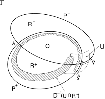
Figure 8: The panel shows the sets $R^{+}$ and $R^{-}$ and their boundaries $P^{+}$ and $P^{-}$ respectively. $U$ is the neighborhood of a regular point where a system of local coordinates $(\xi,\,\eta)$ is introduced. The pre-image of $U\cap R^{-}$ under the return map is shown.

IV.0.1 The structure of the scattering function.

Following the Ref. Eckelt-Zienicke, , we catch the pattern of the scattering map through the map $D$ . In the section $\Gamma$ we give a construction of the sets of orbits with a determined number of crossings through $x=0$. The structure of the sets shows the properties that we have pointed out in the analysis of the hierarchy in the scattering function.

We have already noted that the hierarchy of the regular intervals is established by the number of crossings of $x=0$. This prompts to think that $D$ and its iterates should play a role.

• 

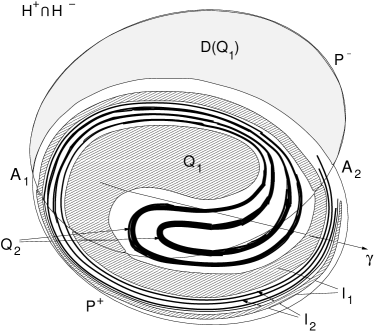
Figure 9: The set $Q_{1}$ is the pre-image of $R^{-}\cap(P^{+}\cup H^{+})$: it is a spiral winding on the boundary $P^{+}$. $Q_{2}$ is the pre-image of $R^{-}\cap Q_{1}$ and it consists of an infinite set of double spirals; two representatives are shown. The sets $I_{i}=Q_{i}\cap(P^{-}\cup H^{-})$, $i=1,\,2$, are also displayed. The line $\gamma$ represents a set of initial conditions ($x_{0}=0,\,p_{0}$) of orbits that get a map of type of fig. 1.

Consider the sets

$$\begin{split}Q_{n}&=\{(p,\,\tau)\ :\ D^{k}(p,\,\tau)\in R^{+}\ \ \ k=0,\,1,\,\ldots\ n-1\ ,\\ &\quad\ D^{n}(p,\,\tau)\in(P^{+}\cup H^{+})\}\end{split}$$ (11)

i.e. $x(t;\,p,\,\tau)$ escapes to a state of scattering after at least $n+1$ zeros. $Q_{n}$ is non-empty. We want to understand the arrangement of the sets $Q_{n}$ in the domain $R^{+}$

We start by noting that $D(Q_{1})=R^{-}\cap(P^{+}\cup H^{+})$  (see fig. 9). The arc $A_{1}A_{2}$ of the boundary of $R^{-}\cap(P^{+}\cup H^{+})$ intersects $P^{-}$ transversally at the regular points $A_{1}$ and $A_{2}$; therefore its pre-image is a double spiral in $R^{+}$ as coming from $P^{+}$ as approaching to it. The double spiral separates $Q_{1}\subset R^{+}$ from $R^{+}\setminus Q_{1}$. It is straightforward to see that $D(Q_{2})=Q_{1}\cap R^{-}\subset(R^{+}\cap R^{-})$. It follows that $Q_{2}\subset(R^{+}\setminus Q_{1})$. The set $Q_{1}\cap R^{-}$ consists of an infinity of components that accumulate to $P^{+}$. Except, possibly, for a finite number, each of the components meet $P^{-}$ transversally on both ends. As above, each stripe is mapped by $D^{-1}$ to a loop spiraling twice against $P^{+}$ (from the property (10)) and that, again, crosses $P^{-}$ transversally. Hence $Q_{2}$ is an infinity of double spirals (see fig. 9). The tail of $Q_{1}$ is located between the branches of each double spiral; the sequence of these double spirals accumulates to the boundary of $Q_{1}$.

This construction is repeated indefinitely. We find that $Q_{n}=D^{-1}(Q_{n-1}\cap R^{-})$, $n\in\mathbb{N}$, is an infinite set of double spirals and each one of these is the image, under $D^{-1}$, of a strip in $R^{-}\cap R^{+}$, transversally met by $P^{-}$. Between the two tails of a double spiral of $Q_{n-1}$ there is an infinity of double spirals of $Q_{n}$. In fact, we next show that $Q_{n}\subset R^{+}\setminus(\cup_{m=1}^{n-1}Q_{m})$. Let us assume $Q_{n}\cap Q_{n-k}\neq\emptyset$, $k=1,\,2,\,\ldots,\,n-1$. We take $D^{n-k}(Q_{n})$ and $D^{n-k}(Q_{n-k})$ and we conclude that  $(Q_{k}\cap R^{-})\cap((P^{+}\cup H^{+})\cap R^{-})\neq\emptyset$ . This conclusion is false because $Q_{k}\subset R^{+}$. Finally, $Q_{n-1}$  and $Q_{n}$ are dis-joined because they are images, under $D^{-1}$, of dis-joined set.

We focus on the set $I_{n}=Q_{n}\cap(P^{-}\cup H^{-})$, i.e. we consider solutions with a finite number of zeros. They are parabolic or hyperbolic for $t\rightarrow+\infty$ and for $t\rightarrow-\infty$.
For all $n$ , $I_{n}$ is a subset of $R^{+}\setminus R^{-}$. From the above construction for all $n\in\mathbb{N}$ between two stripes $I_{n}$ there is an infinity of stripes $I_{n+1}$.

We are now able to explain the structure of the scattering maps (like fig. 1). We carry out the fig. 1 by fixing the initial position ($x(0)=0$) and scanning an outgoing variable (the energy $H_{0}$) as a function of the initial velocity. In the plane $\Gamma$ the organization of the scattering map (see figures 2-5) is connected to the pattern of the intersections of the set $\cup_{n}I_{n}$ with the radial line $\tau=0$ (see fig. 10). In fig. 9 the radial line $\tau=0$ is denoted by $\gamma$.

Note that the construction of fig. 10 is analogous to the construction of a Cantor set. In the first stage one removes a countable number of intervals $I_{1}$ that accumulate to $P^{+}$. In the second stage from each remaining interval a countable number of subintervals converging to both the ends of the interval are removed, and so on.

• 

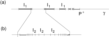
Figure 10: The structure of the intersections with a line $\gamma$, transversal to the boundary $P^{+}$. In $(a)$ it is shown the set $\{I_{1}\}$ of intervals cut out on the spiral $Q_{1}$. The plot $(b)$ displays the intervals $I_{2}$ cut out on the infinite number of double spirals between two branches of the tail of $Q_{1}$. 

The return map provides a construction of an arrangement of sets in the phase space that strongly reminds us the hierarchical structure of the scattering function. The analysis is qualitative but effective.

The scattering map could play a more important role. In the Refs. alekseev, and Eckelt-Zienicke, the authors analyze models with scattering by a one dimensional, periodically oscillating potential well. They construct a set $\Lambda$ which is invariant under $D$ and the dynamics of $D$ in $\Lambda$ is topologically conjugated to a symbolic dynamics; thus they conclude that their models show chaotic scattering. The potential is attractive with respect to the origin for all times; by means of this property they control the dynamics in the vicinity of the parabolically escaping orbits. This control is essential to establish that the return map is locally a horseshoe map and that $\Lambda$ is a (non compact) Cantor set.

V The fractal structure of the delay time function and the algebraic decay law.

• 

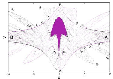
Figure 11: There are shown the stable manifolds (black) and the unstable ones (red) of the outermost fixed points $A$ and $B$. They are determined through the method of sprinkler. The fundamental region $\mathcal{A}$ is the ’rectangle’ $AA_{1}BB_{1}$. $a_{i}$ and $b_{i}$  $i=1,\,2$, are the stable tendrils of $A$ and $B$, respectively. The points $x_{i}$, $z_{i}$, $i=1,\,2$ mark the tips of the stable gaps of first and second order. The point $u_{1}$ is the tip of the first order unstable gap.

• 

Figure 12: Schematic plot of a complete horseshoe. The outermost fixed points are labeled $A$ and $B$. The rectangle $AA_{1}BB_{1}$ is the fundamental region $\mathcal{A}$. There are displayed gaps up to order three. The point $x_{i}$ is the tip of the stable gap of $B$ of $i-th$ order. The point $t_{i}$ is the tip of the stable tendril of $A$ of $i-th$ order. $z_{1}$ and $u_{1}$ label, respectively, the tip of stable and unstable first gap of $A$.

V.1 The fundamental region and the invariant manifolds.

We are addressed to give a connection between the delay time of a trajectory and the number of steps that it performs in a given region of the phase space (in this section we deal with the periodic driver ($f=f_{2}=\sin(\nu\,t)$). In order to do this we use some ideas of Ref. Jung-Lipp-Seligman, and Ref. Emmanouilidou, . The considered region is a part of a phase space which contains the invariant set of the scattering process. Its boundaries are traced out by the segments of the invariant manifolds corresponding to the outermost fixed points in position space. Some non-hyperbolic areas may be found in the region.

We determine the invariant manifolds (the stable manifold $W_{s}$ and the unstable one $W_{u}$) by means of the ’sprinkler algorithm’ that was introduced in Ref. KG85, . The method consists in considering a distribution of initial conditions from a region that contains the chaotic set. Each trajectory is followed until a given time $t$ large enough. If the initial point is close enough to the stable manifold it spends a time larger than $t$ to escape from the given region along the unstable manifold. Therefore the initial points, that still stay in the region at $t$, form the stable manifold and the set of points at time $t$ forms the unstable manifold.

The fig. 11 gives the result of the numerical calculation; we use a grid of $20000\times 6000$ initial points: the stable manifolds are shown in black and the unstable ones are shown in red. We focus on the diamond-shaped area $AA_{1}BB_{1}$ that we name fundamental region and denote by $\mathcal{A}$. The points $A$ and $B$ are the outermost saddle points respectively at $x>0$ and $x<0$. There is an elliptic fixed point close to the origin; it is encircled by KAM tori, secondary elliptic points and other possible invariant structures that are remnant of the quasi-periodic case. Altogether these structures determine a region of phase space where the dynamics is not hyperbolic.

The Hamiltonian (5) is not invariant under the transformation $x\rightarrow x^{\prime}=-x$; therefore the underlying invariant structure seen by the particle is different when it comes from opposite directions. However the Hamiltonian is invariant under the composition of $t\rightarrow-t$ and $x\rightarrow-x$; it follows that, in the resultant pattern of fig. 11, we convert each stable manifold to an unstable one and vice versa by letting $x\rightarrow-x$.

The intertwined structure of fig. 11 is obtained by starting from the segments of the manifolds $W_{s}$ and $W_{u}$ that make up the boundaries of $\mathcal{A}$. The homoclinic/heteroclinic intersection points between $W_{s}$ and $W_{u}$ belong to the chaotic set and the topology of the intersections determines the structure of the outermost component of the set.

The fig. 12 gives a schematic plot of the intersections set of the invariant manifolds of $A$ and $B$ (we do not consider chaotic structures owing to inner fixed points). It is the known construction of the Smale horseshoe: the fundamental region $\mathcal{A}$ (whose boundaries $AA_{1}BB_{1}$ are given by segments of the invariant manifolds of the outermost fixed points $A$ and $B$) is stretched and folded back onto itself. We fold $\mathcal{A}$ two times because we have two fixed points.

We now describe in more detail the construction of fig. 12. The segments of the boundaries of the fundamental region (the unstable segments $AA_{1}$ and $BB_{1}$ and the stable ones $AB_{1}$ and $BA_{1}$) are called tendrils of zero order. We propagate the segments of the stable manifolds backward in time and the segments of the unstable manifolds forward. We focus on the stable manifold of the fixed point $B$ and the local segment of the unstable manifold of $A$. The pre-images (images) of the stable (unstable) tendrils of zero order are tendrils of first order (the segment $A_{1}t_{1}1$ of $W_{s}$ is the tendril of order one); generally the tendril of order $n$ is mapped to that of order $n+1$ (the arc $2t_{2}3$ of $W_{s}$ is the tendril of order two and it is the pre-image of $A_{1}t_{1}1$).

In between these segments of $W_{s}$ forming the tendrils there are other segments $g_{n}^{B}$ of $W_{s}$ going across the fundamental region; they are called gaps of order $n$. $g_{1}^{B}$ is the arc $1x_{1}2$. The points of $g_{1}^{B}$ are mapped to the segment $3x_{2}4$, i.e. the stable second order gap $g_{2}^{B}$. Generally the pre-image of $g_{n}^{B}$ is the gap $g_{n+1}^{B}$. We may similarly proceed with the invariant manifolds of $B$; the segment $5z_{1}6$ is the first gap $g_{1}^{A}$ of $W_{s}$ of the fixed point $A$; $7z_{2}8$ and $9z_{3}10$ are the gaps $g_{2}^{A}$ and $g_{3}^{A}$, respectively, and so on.

In this construction we use the invariant manifolds of the fixed points on the corners of $\mathcal{A}$ ($A$ and $B$). This choice implies a favorable property which does not hold in the case of the invariant manifolds of periodic points lying in the interior of $\mathcal{A}$. In fact the gaps which are cut into $\mathcal{A}$ by the manifolds of $A$ and $B$ are regions of $\mathcal{A}$ which do not cover the invariant set; no higher level segment of $W_{s}$ will ever enter such gaps. Furthermore it holds: the topology of the intersections is determined by the intersection pattern between all the tendrils of the stable manifolds and the ’local’ segments of the unstable manifolds, i.e. the branches $AA_{1}$ and $BB_{1}$ in the fig. 11. This fact can be easily understood if we think that each intersection (homoclinic, heteroclinic) point in $\mathcal{A}$ is the image-pre-image of an intersection point of $W_{s}$ with the local segments.

The horseshoe construction is complete when the tip $u_{1}$ of the first order gap of the unstable manifold reaches the other side of the fundamental area (the schematic plot of fig. 12 shows a complete horseshoe). In this case a stable gap of order $n$ reaches into all tendrils up to the order $n$. The fig. 13 shows a partial development of the pattern of gaps in a tendrils of order $n$. The innermost part is a gap of order $n$. Between this middle gap and the boundary of the tendril there are two gaps of order $n+1$. On the next level there are two gaps of order $n+2$ in between each pair of adjacent gaps of lower order or between the gaps of lower order and the boundary. This scheme continues to higher level. In a tendril of order $n$ we find $2\times 3^{n_{1}-1}$ gaps of order $n+n_{1}$. Between any two adjacent gaps of the same order we find gaps of order arbitrarily high; hence in each neighborhood of a gap we find gaps of all orders high enough. In the area enclosed between a tendril and the local segment the gaps fill a subset of null measure. The resultant structure is a set of segments of $W_{s}$ along the direction of the tendril whose sections in the transverse direction are Cantor sets. This structure is closely connected to the invariant set in the fundamental region.

The link between the gaps and the scattering problem is due to the following mechanism. The tendrils reach out into the incoming asymptotic region. We consider a particle that comes from far away and approaches the local segment and lies in a gap of a tendril of order $n$. Except for a fractal set of lines (resembling the invariant set) the particle is mapped to a point of a gap in $\mathcal{A}$. In fact, by the construction of the horseshoe, any point in the stable tendril of order $n$  is mapped in the stable tendril of order $n-1$. The first order tendril of the stable manifold of $A$ ($t_{1}^{s}$) is mapped in the first gap of the unstable manifold of $B$ ($u_{1}$); more specifically, a point in a stable gap of order $n$ ($g_{n}^{s}$) in $t_{1}^{s}$ is brought into $u_{1}\cap g_{n-1}^{s}$ . Points of a gap are brought out of the fundamental region after a finite number of iterations of the dynamical map: the stable gap $g_{n}^{s}$ is mapped to $g_{n-1}^{s}$ and the image of $g_{1}^{s}$ is the first order unstable tendril of $B$. At this point the particles leaves out of $\mathcal{A}$; in fact an unstable tendril of order $n$ is mapped to an unstable tendril of order $n+1$, and so on. Finally, except for a set of zero measure, a scattering trajectory experiences a finite number of steps inside the fundamental area whenever it approaches the local segment of the unstable manifold along a gap in a stable tendril.

From these considerations we assert that the arrangement of singularities of a scattering function should be related to the structure of the chaotic invariant set and then to the sequence of tendrils along the local segment of the unstable manifold. In this sense we can reconstruct the structure of the horseshoe from the measure of the scattering functions, i.e. from asymptotic measurements.

• 

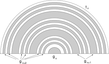
Figure 13: The plot displays the first few stages of the development of the pattern of gaps in a tendril of order $n$.

V.2 The scattering function and the structure of the invariant sets of the outermost fixed points.

We know that the set of singularities of a scattering function shows how the line of the incoming particle asymptotes pierces the bundle of stable manifolds of the chaotic invariant set. However we may state that the main properties of a scattering function are dominated by the component of the invariant set due to the outermost fixed points.
We focus on the delay time scattering function; we keep the initial position fixed and vary the initial velocity and for the corresponding trajectories we monitor the time interval $\tau$ between the first and the last zero. The plot $(a)$ of fig. 14 shows a typical pattern. The structure of the delay time closely corresponds to the structure of the $N_{c}$ scattering function (compare $(a)$ with $(b)$):

• an interval with a given number of zeros is related to a continuous branch of the delay time function;

• each regular interval of $\tau$ is accumulated by a sequence of regular intervals for $\tau$ going to arbitrary large values.

We are mainly interested in the singularity structure of the scattering functions. For this particular purpose the information provided by $\tau$ is the same as the time interval which the particle spends in the fundamental region.

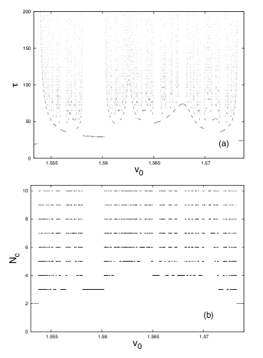
Figure 14: The plot $(a)$ displays the delay time scattering function for the same line of initial conditions of $(b)$ fig. 1. The plot $(b)$ is the number of crossings of $x=0$ in the same conditions of $(a)$.

We have focused our attention on the features of the dynamics of particles approaching the fundamental region through the local unstable segment. Our considerations drive us to affirm that the singularities structure in $\tau$ is correlated with the structure of intersections of $W_{s}$ of a fixed point with the local branch of $W_{u}$ of the other fixed point, i.e. the pattern of fig. 13.

On account of the structure of gaps in a tendril, we see that, except for a set of zero measure, the trajectories, coming from a line of initial conditions and intersecting the tendril, are mapped far away after they undergo a finite number of iterates inside the fundamental region. A trajectory that approaches the fundamental region along a gap belongs to a regular interval of the delay time function. On the other hand the set of singularities of the delay time function corresponds to the set of points in a tendril that do not belong to any gaps; the trajectory is confined forever inside the fundamental region.

The graph of $\tau$ possesses the following hierarchical organization. Consider the connection between $\tau$ and $N_{c}$. In the graph $(b)$ of fig. 14 we remove all continuous branches corresponding to the intervals with the lowest $N_{c}$; the $\tau$ structure is separated into substructures that are similar to the parent one; each removed subinterval is surrounded by smaller subintervals with a higher value of $\tau$ (’castle-like’ structure; see Ref. Ruckerl-Jung, ). We may iterate the procedure and the number of zeros fixes the level of cutting out; at each step we get a generation of substructures similar to that of the previous generation. In this way we determine a hierarchical organization. It is important to observe that the pattern of gaps in a tendril (fig. 13) displays the same organization. In a tendril of order $n$, whenever we cut a gap of order $n+1$ away, the pattern is separated into substructures, with gaps of higher order, similar to each other. We may iterate the method for gaps of higher order; the hierarchy follows the order of the gap. In this way we establish a connection between the pattern of the delay time function and the structure of the $N_{c}$ scattering function (compare $(a)$ and $(b)$ of fig. 2). Likewise the qualitative approach that refers the return map, in this section we have examined some features of the scattering function using global considerations on the dynamics (the invariant manifolds of the fixed points $A$ and $B$). In addition we have not needed to take into account all the chaotic invariant set.

V.3 The algebraic decay.

• 

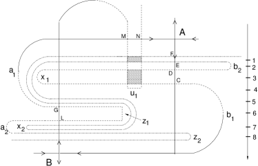
Figure 15: Schematic plot of the scenario in fig. 11. The horseshoe is incomplete and asymmetric; the first order unstable gap (tip $u_{1}$) does not reach the opposite side of the fundamental area. The numbers in the right column count all gaps up to order two. The horseshoe is characterized by the development parameters $\gamma_{A}=1/3$ and $\gamma_{B}=1$.

In section 2, we have checked an algebraic law both for $N(t)$, the decay with time of the number of temporarily bound orbits, and for $N(n)$, the distribution of zeros. Hyperbolic systems usually exhibit $N(t)$ to have an exponential decay law Grebogi-Ott-Yorke ; Kovacs-Tell . The algebraic decay would press to consider our system to be non-hyperbolic Lai-Ding-Grebogi-Blumel ; Meiss-Ott or, if it were hyperbolic, there should be a special mechanism that makes the decay slower than what is expected when the KAM tori structure is completely broken Lee ; Vivaldi-Casati-Guarnieri . Our problem should fall in with the non-hyperbolic situation. In fact the Poincaré map shows orbits that curl up tori, i.e. there is a mixture of motion close to the deformed tori and motion far away from them.

The presence of KAM surfaces affects the particle motion in the nearby chaotic regions; even if the particle starts in a chaotic region, sooner or later the particle approximates the surface and wanders close to it for a long time; it is the ”stickiness effect”. The motion in a KAM surface is quasi-periodic and hence, nearby the tori, the Lyapunov exponents in the directions along the surface are zero. Moreover, in our case, the Poincaré map is symplectic (the driver is periodic) and, because it is two-dimensional, the Lyapunov exponent perpendicular to the surface also has to be zero. The stickiness effect reduces the transport of orbits initialized in a chaotic region and explains the algebraic decay law instead of the exponential one. In the Ref. Lai-Ding-Grebogi-Blumel, it is established that the size of the decay depends on the complexity of the pattern of island chains: the more dominant the island chains in the chaotic region, the slower the escape process.

We have remarked that in the Ref. Beeker-Eckelt, an algebraic decay for the delay time function is obtained. Nevertheless in this case the effects of the KAM components are negligible. When we consider $V=V_{2}$, $V_{2}\sim|x|^{-2}$ for $|x|\gg 1$, the explanation of Beeker et al., applied to our case, supplies a decay law slower than the law we observe. The reasoning of Beeker et al. attaches the most part of the importance to the orbits that spend the most part of time far away from the interaction region; they are trajectories which almost escape after e.g. the $n$-th zero, but are eventually recaptured, so that there is a long time elapsing between the $n$-th and the $(n+1)$-th zero. Because of the KAM surfaces, in our case we have to take into account the orbits that run inside the interactions region. Their ’life-time’ is shorter than that of the temporarily bound orbits close to the parabolic one; in fact the energy absorptions mainly take place around the origin. On the basis of these considerations we expect the algebraic decay to be faster than the scaling determined by the class of orbits in the approximation of Ref. Beeker-Eckelt, . In order to give a quantitative characterization of the development stage of the horseshoe construction a parameter $\gamma$ (’development parameter’) was introduced in Ref. Ruckerl-Jung, . For the system under consideration there are three most effective fixed point: the outermost ones and the inner elliptic fixed points. The development parameter for the corresponding horseshoe is $\gamma=r_{n}\ 3^{-n}$; $n$ is the highest order of the gap we consider and $r_{n}$ is the order of gap, which the tip of the first unstable gap reaches, when we count the gaps from the fixed point (see Ref. Jung-Lipp-Seligman, ). Note, the value of $\gamma$ does not depend on the choice of the order $n$ we consider.

The parameter allows to evaluate how deep the first order gap penetrates into the fundamental area of the horseshoe compared to the complete case; in the development of a horseshoe the parameter $\gamma$ varies from 0 to 1. A horseshoe is complete whenever the unstable gap of order one reaches the opposite side of the fundamental area (see fig. 12); in this case $\gamma=1$.

The parameter is used to qualitatively characterize the topology of the homoclinic/heteroclinic tangle of the outer fixed points. It remains the same when under variations of physical parameters the changes of the topology concern tangencies of branches of manifolds of level high enough. It is important to point out the relation of $\gamma$ to the topological entropy $K_{0}$. In Ref. Ruckerl-Jung, it is obtained, by numerical computation, that $K_{0}$ is a monotonic function of $\gamma$. The parameter ignores the unique aspects of the KAM surfaces; it does not take into account the winding numbers of the elliptic points and neglects effects coming from the invariant manifolds that penetrate into the surroundings of the KAM islands. However the parameter considers the part of the invariant set which is the most important for the scattering function.

We focus on the fig. 11. We observe that the inner non-hyperbolic island obstructs the penetration of the unstable gap in the fundamental area and keeps from the complete growth of the saddle pattern. The fig. 15 is a schematic plot of fig. 11; the stable manifolds of $A$ and $B$ are plotted up to order two and $W_{u}$ of the point $B$ is plotted up to order one. The numbers in the right column count all gaps up to order two, consecutively from the top to the bottom. We note that the horseshoe is non-symmetric and hence it is incomplete. Actually the first unstable gap of $A$ reaches the other side of the fundamental region (it is the mirror image of $x_{1}$) and the unstable gap $u_{1}$ does not. The horseshoe is thus described by two development parameters. The parameter value of $W_{u}$ of $B$ is $\gamma_{B}=1$. On the other hand, when we consider gaps up to second order ($n=2$) the $u_{1}$ ends in the third gap from the top ($r_{2}=3$), thus leading to $\gamma_{A}=1/3$.

Concerning the scattering problem, the effects of KAM islands and their secondary structures should have little influence on the approximation of the horseshoe reconstruction: they are connected to the penetrations of the invariant manifolds of the outermost fixed points in the secondary structures around the KAM islands. In non-hyperbolic case the KAM component obstructs a full development of the horseshoe. In contrast to the complete horseshoe (fig. 13) in the incomplete case some inner gaps in a tendril can disappear (fig. 15). However the non transversal intersections between stable and unstable manifolds due to KAM tori have small effects on the scattering functions Ruckerl-Jung , i.e. on the structure of the intersections between the stable manifold and the local segment of the unstable manifold. For $\nu=0.8$ and $e_{0}=1$  there are tangencies for gaps of order $n\geq 3$. The effects of the tangencies are visible on the scattering functions at the order $2\,n\geq 6$; in fact whenever the $n$-th order stable gap is tangent to the $n$-th unstable gap then the $(n+1)$-th order stable gap intersects the $(n-1)$-th unstable gap and, finally, the $(2\,n)$-th stable gap intersects the local segment at the $(2\,n)$-th tendril.

VI Scattering features as the driver amplitude is varied.

In this section we fix the initial conditions and vary the parameter $e_{0}$. We know (see Ref. Ding-Grebogi-Hott-Yorke, ) that a scattering system can experience transitions from regular to chaotic scattering as a parameter of the system is varied. The onset of chaotic scattering can be achieved through combination of bifurcation mechanisms: new periodic orbits are added and their stable and unstable manifolds intersect each other. These events cause changes in the chaotic set; as the parameter is varied the hyperbolic component increases and the formation of structures topologically equivalent to a horseshoe may occur.

We do not address the question of how the chaotic scattering arises as $e_{0}$ changes. We only discuss the qualitative behavior of the outgoing energy of a trajectory with given initial conditions. We argue that the main properties are connected to the invariant pattern caused by the outermost fixed points. We consider both the periodic case ($f=f_{2}$) and the finite duration driver ($f=f_{1}$). The initial conditions are set $x(0)=0$ and $\mathrm{v}(0)=1.049$ ($H_{0}=0.55$ at $e_{0}=0$).

In the case of $f=f_{1}$ the map links $e_{0}$ to the value of $H_{0}$ taken at $t^{\ast}$ , after the driver is switched off (see fig. 16):

$$S^{1}_{(x_{0},v_{0})}:\ \ e_{0}\ \,\mapsto\ \,H_{0}(p(t^{\ast}),\,x(t^{\ast}))$$

For the periodic driver we introduce the one-to-many values mapping:

$$S^{2}_{(x_{0},v_{0})}:\ \ e_{0}\ \,\mapsto\ \,H_{0}(p(t_{k}),\,x(t_{k}))$$

$\,\nu\,t_{k}=\pi/2\,+\,k\,2\,\pi$, $k=1,\,2,\,\ldots$; the map links $e_{0}$ to the energies  $H_{0}$, every driver period. In all cases we obtain patterns that display some of the features of the maps investigated above:

• There is a sequence of alternating regular and irregular intervals of $e_{0}$.

• A magnification of an irregular interval shows a pattern similar to the complete one (see $(b)$ of fig. 16).

• Except for very few cases a regular interval corresponds to a determined number of crossings of $x=0$ (or number of steps in the fundamental region. See $(c)$ of fig. 16).

We should point out that, differently from sect. $3$, the hierarchy of the regular intervals with respect to $N_{c}$, the number of crossings of $x=0$, does not completely hold. In fact, there are some regular intervals where $N_{c}$ changes value (see the jump from $N_{c}=5$ to $N_{c}=7$ of the regular interval at the left hand side of the plot $(d)$ of fig. 16 and the jump from $N_{c}=8$ and $N_{c}=10$ of the regular interval $[4.954,4.957]$).

Figure 16: The plot $(a)$ displays the asymptotic-out energy ($H_{0}$) vs the driver amplitude ($e_{0}$) for $f=f_{1}$. The plot $(b)$ is a magnification of the marked interval of $(a)$. The plot $(d)$ shows $N_{c}$ corresponding to the interval of $e_{0}$ in the plot $(c)$

We come back to the horseshoe construction that is traced out by the invariant manifolds of the outermost fixed points. We have stated that, for fixed $e_{0}$, the topology of homoclinic/heteroclinic intersections determines the structure of a scattering function corresponding to a line of initial conditions which cuts tendrils of the stable manifold close to the local branch. We want to explain what occurs when we fix the initial conditions and vary $e_{0}$. By changing $e_{0}$ the length of manifolds is affected and homoclinic bifurcations take place whenever the branches of two manifolds cross each other. Accordingly the invariant set changes its topology and some orbits may get lost.

Consider $(a)$ of fig. 17: a tip $u_{1}$ reaches into a stable gap that, we know, is free of further gap of $W_{s}$, and the tips $z_{1}$ and $x_{2}$  lie in the areas of tendrils. In these situations stretching or compression of segments of manifolds do not cause any tangencies. If this is the case for the tips of all gaps up to order $n$ then, even if we vary $e_{0}$ over a suitable interval, the corresponding changes of the topology may affect only orbits with at least $n$ iterates in the fundamental region. This implies a stability of a part of the structure of orbits against bifurcations.

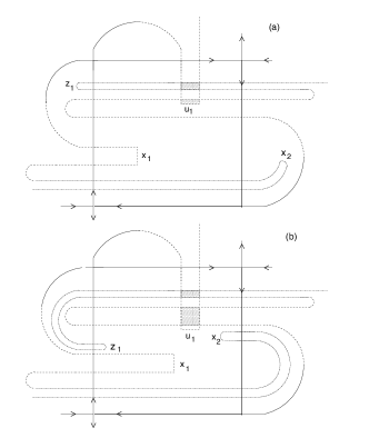
Figure 17: The plot $(a)$ displays an incomplete horseshoe where the tips $u_{1}$, $x_{2}$ and $z_{1}$ enter areas where they cannot hit invariant manifolds. In the plot (b) the same tips can undergo tangencies under small changes of $e_{0}$.

On the other hand a tip that exits a gap can undergo a homoclinic tangency for small changes of $e_{0}$ (see $(b)$ of fig. 17). In the fundamental region, the structure of the gaps, that is kept fixed over an interval of $e_{0}$, resembles the structure of homoclinic/heteroclinic intersections that is ”seen” by a line of initial conditions, as long as we consider orbits with a number of steps in $\mathcal{A}$ not too large. The second structure is connected to the pattern of gaps in a tendril. We conclude that the structure of singularities of the maps $S^{i}_{(x_{0},v_{0})}$, $i=1,\,2$, should resemble to the scattering functions with respect to a line of initial conditions.

An essential observation is that there are parameter intervals in which the tips of the invariant manifolds do not create homoclinic bifurcations under small changes of the parameter. This occurs due to the gaps which are empty of invariant manifolds. It should be pointed out that the idea of the gaps may be helpful only if it is applied to a system with an open, infinite phase space (scattering systems). In fact in a bound Hamiltonian system the invariant manifolds are dense in a connected subset of the phase space not containing KAM tori.

VII Conclusions.

We have studied a one-dimensional oscillator, with a single equilibrium point and critical points at infinity, driven by a force that is either periodic or lasting a finite time interval.

By numerical simulations we have determined maps of scattering data (energy, delay time) and number of zeros of the orbits as functions of an initial condition (the other initial condition and the driver amplitude being kept fixed) and of the driver amplitude (the initial conditions being fixed). The maps display a characteristic pattern. The outgoing variables are smooth functions in intervals where the number of zeros $N_{c}$ of the solutions does not vary; $N_{c}$ marks each interval. Successive removal of all the smooth intervals with $N_{c}=1,\,2,\,3,\,\dots$ leads to a set of singularities that appears to be Cantor-like and corresponds to trajectories that never escape.

The number of zeros plays the role of an order parameter that corresponds to a hierarchical structure of the regular intervals. The same ordering is provided by the delay time function. This property is connected to the structure of gaps in a tendril, i.e. the area that is enclosed between a branch of the stable manifold and the local segment of the unstable manifold and that reaches out the fundamental area into the incoming asymptotic region.

The regular intervals and the singularities pattern of the maps $S^{i}_{(x_{0},\,\mathrm{v}_{0})}$, $i=1,\,2$, are understood through the gaps in the fundamental area: some regions of phase space are void of invariant manifolds and homoclinic-heteroclinic intersections cannot take place even if a change of a parameter can produce stretching or compression of manifolds.

We introduce a map (return map) which is defined in a plane $\Gamma$ and describes the dynamics of the crossings of $x=0$. Through the map we can identify a pattern of subsets in $\Gamma$ whose structure is connected to the structure of the scattering map.

The number of orbits as a function of the time of permanence close to the origin decreases slower than expected: it decreases as a power law rather than exponentially. The explanation is due to the fact that the invariant structures are not completely destroyed: some Cantor tori remain, and a reduction in the number of orbits close to the origin is due to a stickiness effect. These orbits starting far from a torus end up near it and remain there, creating correlations between different orbits and therefore decreasing the chaotic effect.

Bibliography

Bibliography

- (1) B. Eckhardt, Physica D 33, 89 (1988).
- (2) C. Jung and H.J. Scholz, J. Phys. A 20, 3607 (1987).
- (3) C. Jung and H.J. Scholz, J. Phys. A 21, 2301 (1988).
- (4) S. Smale, Bull. Am. Math. Soc. 73, 747 (1967).
- (5) B. V. Chirikov and D. L. Shepelyanski, Physica D 13, 394 (1984).
- (6) C. F. F. Karney, Physica D 8, 360 (1983).
- (7) J. D. Meiss and E. Ott, Phys. Rev. Lett. 55, 2741 (1985).
- (8) C. F. Hillermeier, R. Blmel, and U. Smilansky, Phys. Rev. A 45, 3486 (1992).
- (9) A. Beeker and P. Eckelt, Chaos 3, 490 (1993).
- (10) Y. C. Lai, K. Zyczkowski, and C. Grebogi, Phys. Rev. E 59, 5261 (1999).
- (11) J. M. Petit and M. Hénon, Icarus 66, 536 (1986).
- (12) E. Pollack and P. Pechukas, J. Chem. Phys. 69, 1218 (1978).
- (13) B. P. Koch and B. Bruhn, J. Phys. A 25, 3945 (1992).
- (14) R. T. Skodje and M. J. Davis, J. Chem. Phys. 95, 2429 (1988).
- (15) B. Eckhardt and H. Aref, Philos. Trans. Roy. Soc. A 326, 655 (1988).
- (16) H. Aref, J. B. Kadtke, I. Zawadski, L. J. Campbell, and B. Eckhardt, Fluid. Dyn. Res. 3, 63 (1988).
- (17) B. Eckhardt and C.Jung, J. Phys. A 19, L829 (1986).
- (18) C. Jung, J. Phys. A 19, 1345 (1986)
- (19) C. Jung, J. Phys. A 20, 1719 (1987).
- (20) P. Mulser and M. Kanathipillai, Phys. Rev. A 71, 63201 (2005).
- (21) M. Kundu and D. Bauer, Phys. Rev. Lett. 96, 123401 (2006).
- (22) V. M. Alekseev, Math. USSR Sbornik 6, 505 (1968).
- (23) V. M. Alekseev, Math. USSR Sbornik 7, 1 (1969).
- (24) P. Eckelt and E. Zienicke, J. Phys. A 24, 153 (1991).
- (25) J. Moser Stable and randon motion in dynamical systems (Princeton Univ. Press, Princeton, 1973)
- (26) G. Cicogna and M. Santoprete, Regular and Chaotic Dynamics 6, 377 (2001).
- (27) H. Dankowicz and P. Holmes, J. Diff. Eq. 116, 468 (1995).
- (28) G. Haller Chaos near resonance (Springer-Verlag, New York, 1999)
- (29) Y. C. Lai, R. Blumel, E. Ott, and C. Grebogi, Phys. Rev. Lett. 68, 3491 (1992).
- (30) M. Ding, T. Boundis, and E. Ott, Phys. Lett. A 151, 395 (1990).
- (31) C. Jung, C. Lipp, and T.H. Seligman, Ann. Phys. 275, 151 (1999).
- (32) A. Emmanouilidou, C. Jung, and L. E. Reichl, Phys. Rev. E 68, 46207 (2003).
- (33) H. Kantz and P. Grassberger, Physica D 17, 75 (1985).
- (34) B. Rckerl, C. Jung, J. Phys. A 27, 55 (1994).
- (35) C. Grebogi, E. Ott, and J.A. Yorke, Phys. Rev. Lett. 57, 1284 (1986).
- (36) Z. Kovacs and T. Tél, Phys. Rev. Lett. 64, 1617 (1990).
- (37) Y. C. Lai, M. Ding, C. Grebogi, and R. Blmel, Phys. Rev. A 46, 4661 (1992).
- (38) K. C. Lee, Phys. Rev. Lett. 60, 1991 (1988).
- (39) F. Vivaldi, G. Casati, and I. Guarnieri, Phys. Rev. Lett. 51, 727 (1983).
- (40) M. Ding, C. Grebogi, E. Ott, and J. A. Yorke, Phys. Rev. A 42, 7025 (1990).