Seminal magnetic fields from Inflato-electromagnetic Inflation

Abstract

We extend some previous attempts to explain the origin and evolution of primordial magnetic fields during inflation induced from a 5D vacuum. We show that the usual quantum fluctuations of a generalized 5D electromagnetic field cannot provide us with the desired magnetic seeds. We show that special fields without propagation on the extra non-compact dimension are needed to arrive to appreciable magnetic strengths. We also identify a new magnetic tensor field $B_{ij}$ in this kind of extra dimensional theories. Our results are in very good agreement with observational requirements, in particular from TeV Blazars and CMB radiation limits we obtain that primordial cosmological magnetic fields should be close to scale invariance.

I Introduction

Magnetic fields seem to be ubiquitous in the universe. Observations have well established the widespread presence of magnetic fields in the universe 1988A&A…190…41K ; 1989Natur.341..720K ; 1994RPPh…57..325K ; 2002ChJAA…2..293H ; 2002ARA&A..40..319C ; 2004NewAR..48..763V ; 2005A&A…444..739B . Cosmic magnetism has been verified of $\mu$G-order strength in galaxy clusters and also in high redshift protogalactic structures. Recently, in particular, Kronberg et al and Bernet et al reported organized, strong $B$-fields in galaxies with redshifts close to 1.3 2008ApJ…676…70K ; 2008Natur.454..302B . All these seem to suggest that magnetic fields similar to that of the Milky Way are common in remote, high-redshift galaxies. This could imply that the time needed by the galactic dynamo to build up a coherent $B$-field is considerably less than what is usually anticipated. On the other hand, the widespread presence of magnetic fields at high redshifts may simply mean that they are cosmological (pre-recombination) in origin. Although it is still too early to reach a conclusion, the idea of primordial magnetism gains ground, as more fields of micro-Gauss strength are detected in remote proto-galaxies. Recent reviews about primordial magnetogenesis can be found at Kandus Report .

Our work focuses in studying the production of primordial magnetic seeds during an inflationary period, which in turn is induced by the immersion of a particular 4D hypersurface, given by a de Sitter spacetime, in a 5D vacuum space defined on a 5D Riemann-flat extended de Sitter metric. The theory that motivates such scenario is the Induced Matter Theory (IMT)IMT ; imt1 . In this theory inflation can be recovered from the Campbell-Magaard theoremcampbell ; c1 ; campbellb ; campbellc ; campbelld , which serves as a ladder to go between manifolds whose dimensionality differs by one. This theorem, which is valid in any number of dimensions, implies that every solution of the 4D Einstein equations with arbitrary energy momentum tensor can be embedded, at least locally, in a solution of the 5D Einstein field equations in vacuum. Because of this, the stress-energy may be a 4D manifestation of the embedding geometry. Physically, the background metric there employed describes a 5D extension of an usual de Sitter spacetime, which is the 4D spacetime that describes an inflationary expansion.

We will study the simplest inflationary model, that gives us a de Sitter epoch. Electromagnetic studies in this context have been developed previously by 2007Dahia ; 2008Romero ; 2005Liko . To introduce the electromagnetic effects we consider a massless vector field $A_{a}$ of five components. The component normal to the hypersurface has properties similar to a scalar field, so its spectrum, with the Coulomb Gauge, we will see it can only be scale invariant.

In the present paper we consider two types of fields. The first with propagation outside the hypersurface, and the second with the propagation confined to the hypersurface. This last fields need to be generated by some brane source since they produce a discontinuity in the stress tensor. Such distinction is very important since the fields that can propagate outside the hypersurface are strongly suppressed than the usual 4D photon, giving rise to a bluer spectrum. The other fields, in contrast, can give invariant spectrum for magnetic fields. Our results in this way are very similar to 2008JCAP…01..025M .

Additionally, we analyze the electromagnetic fields measured by 4D observers in the effective 4D hypersurface. When we extend our definitions of the relativistic electric and magnetic fields to more dimensions, we obtain new gravitoelectromagnetic fields of scalar and tensorial nature. In our knowledge this is the first time such components are identified in an electromagnetic theory of Brane Worlds or Induced Matter Theory. Finally, it is well known that the spatially flat FRW universe is conformal flat and the Maxwell theory is conformal invariant, so that magnetic fields generated during inflation would come vanishingly small at the end of the inflationary epoch. However, in spatially open FRW models magnetic fields are sufficiently strong to seed the galactic dynamos. The reason is that conformal flatness of the 4D background metric is a global property in spatially flat FRW spacetimes, but a local one in spatially open or closed geometriesb1 ; b2 ; b3 .

This is a very important problem of inflation to explain seminal magnetic fields. The possibility to solve this problem relies in produce non-trivial magnetic fields in which conformal invariance to be broken. The conformal invariance of Maxwell s equations in four dimensions can also be broken if an embedding into a higher dimensional space-time with time-varying extra spatial dimensions is considered. In particular, in Brane Worlds or Induced Matter theory conformal invariance is naturally broken, which make possible the super adiabatic amplification of electric and magnetic field modes during the early inflationary epoch of the universe on cosmological scales.

II Electrodynamics a Riemann-flat extended de Sitter spacetime

We begin considering the action of a free abelian gauge vector field in five dimensions

$$S=-\frac{1}{4}\int d^{5}x\sqrt{{}^{(5)}g}F_{CD}F^{CD};$$ (1)

where $F_{CD}=\nabla_{C}A_{D}-\nabla_{D}A_{C}=\partial_{C}A_{D}-\partial_{D}A_{C}$ is the antisymmetric field tensor. The Maxwell equations of motion in five dimensions are

$$\nabla^{C}F_{CD}=0.$$ (2)

We introduce these fields in a background 5D spacetime in vacuum state. Using some ideas of the Induced Matter Theories we want to obtain a hypersurface that undergoes an effective inflationary period. In this sense we do a the semiclassical expansion of the vector fields

$$A^{C}=\bar{A}^{C}+\delta A^{C},$$ (3)

where the overbar symbolizes the 3D spatially homogeneous background field consistent with the fixed background homogeneous metric and $\delta A^{C}$ describes the fluctuations with respect to $\bar{A}^{C}$. A more detailed explanation can be found in mb2 . This space will be a 5D extension of a 4D de Sitter spacetime, which is very relevant to inflationary cosmology, and is given by a 5D (canonical Riemann-flat) metric with a line elementLedesma2003

$$ds^{2}=\psi^{2}dN^{2}-\psi^{2}e^{2N}d\mathbf{r}^{2}-d\psi^{2},$$ (4)

where $N$ is a dimensionless time like coordinate related with the number of e-folds during a de Sitter inflationary expansion. The 3D space like cartesian dimensionless coordinates $d\mathbf{r}^{2}=dx_{1}^{2}+dx_{2}^{2}+dx_{3}^{2}$ when taking a constant foliation coincide with the 3D space coordinates of the effective 4D hypersurface. The extra (non compact) space-like coordinate $\psi$ has spatial dimension. Instead of these coordinates, we shall use new conformal ones [see appendix (A)], such that

$$ds^{2}=b(w)^{2}\left[a(\eta)^{2}\left(d\eta^{2}-d\mathbf{R}^{2}\right)-dw^{2}\right],$$ (5)

where the scale factors $b(w)=e^{H_{0}w}$ y $a(\eta)=-\frac{1}{H_{0}\eta}$ are dimensionless. The components of the coordinates $(\eta,\mathbf{R},w)$ have spatial dimensions. The foliation $\psi=\psi_{0}$ corresponds with $w=w_{0}=0$ in these coordinates, such that $b(w_{0})=1$.

The volume factor of the manifold is $\sqrt{{}^{(5)}g}=b^{5}a^{4}=\frac{e^{5H_{0}w}}{H_{0}^{4}\eta^{4}}$, and the non zero connections are

$$\Gamma_{\mu\nu}^{0}=-\eta^{-1}\delta_{\mu\nu},\hskip 28.45274pt\Gamma_{AB}^{4}={e^{-2H_{0}w}H_{0}}g_{AB},\hskip 28.45274pt\Gamma_{\mu 4}^{\nu}=H_{0}\delta_{\mu}^{\nu}.\hskip 28.45274pt$$ (6)

The equations (2) in these coordinates are

$$-\left[\eta^{2}\partial^{2}+\frac{1}{H_{0}^{2}}\left(\frac{\partial^{2}}{\partial w^{2}}+H_{0}\frac{\partial}{\partial w}\right)\right]A_{0}+\eta^{2}\frac{\partial}{\partial\eta}\partial_{i}A_{i}+\frac{1}{H_{0}^{2}}\frac{\partial}{\partial\eta}\left(\frac{\partial}{\partial w}+H_{0}\right)A_{4}=0,$$ (7)

$$\left[\eta^{2}\left(\frac{\partial^{2}}{\partial\eta^{2}}-\partial^{2}\right)-\frac{1}{H_{0}^{2}}\left(\frac{\partial^{2}}{\partial w^{2}}+H_{0}\frac{\partial}{\partial w}\right)\right]A_{j}+\eta^{2}\partial_{j}\partial_{i}A_{i}+\frac{1}{H_{0}^{2}}\partial_{j}\left(\frac{\partial}{\partial w}+H_{0}\right)A_{4}=0,$$ (8)

$$\left(\frac{\partial^{2}}{\partial\eta^{2}}-\frac{2}{\eta}\frac{\partial}{\partial\eta}-\partial^{2}\right)A_{4}+\frac{\partial}{\partial w}\partial_{i}A_{i}+\frac{\partial}{\partial w}\left(\frac{2}{\eta}-\frac{\partial}{\partial\eta}\right)A_{0}=0,$$ (9)

where $\partial^{2}$ is the ordinary Laplacian operator.

We adopt the usual Coulomb Gauge for the study of the electromagnetic effects on the hypersurface: $A_{0}=0$ y $\partial_{i}A^{i}=0$. The equation for the temporal component $A_{0}$ remains as a constraint equation for $A_{4}$,

$$\frac{\partial}{\partial\eta}\left(\frac{\partial}{\partial w}+H_{0}\right)A_{4}=0.$$ (10)

Notice that in a 5D Minkowskian metric: $dS^{2}=\eta_{ab}dx^{a}\,dx^{b}$, the connections vanish and the field equations remain decoupled after the gauge choice. In this case the universe does not expands so that the inflaton field $A^{4}=0$.

To continue we propose the ansatz

$${A^{C}}(\eta,\mathbf{R},w)=e^{mH_{0}w}{A}_{m}^{C}(\eta,\mathbf{R}),$$ (11)

where $m$ can be any complex number. In particular, to make a Fourier expansion base functions, we shall consider the allowed values $m=-1/2+ip$, where $p=P/H_{0}$ are the wave numbers of the field in the $w$ direction per unity of $H_{0}$. The reason to make it relies in that $\sqrt{g}=e^{5H_{0}w}\eta^{-4}$ and $F_{AB}F^{AB}\propto e^{-4H_{0}w}$, so that we obtain $\int d\eta\,\int d^{3}x\,dw\,e^{H_{0}w}(\cdots)$ in the action. This exponent should be suppressed in order to address a correct Fourier expansion in terms of $e^{iPw+i\mathbf{k}\cdot\mathbf{R}}$.

It is also important to consider particular solutions of perturbative order, without the oscillatory regime with respect to the extra coordinate. These solutions are described by the real values of $m$. In any case the equations are

$$(1+m)\frac{\partial}{\partial\eta}A_{4m}=0,$$ (12)

$$\left[\eta^{2}\left(\frac{\partial^{2}}{\partial\eta^{2}}-\partial^{2}\right)-m(m+1)\right]{A_{j}}_{m}+\left(m+1\right)\partial_{j}{A_{4}}_{m}=0,$$ (13)

$$\left(\frac{\partial^{2}}{\partial\eta^{2}}-\frac{2}{\eta}\frac{\partial}{\partial\eta}-\partial^{2}\right){A_{4}}_{m}=0.$$ (14)

We notice from (12) that the only possible mode for $A_{4m}$ that can exist is $m=-1$. The others yield $\partial^{2}A_{4}=0$, such that $A_{4m}=0$ when we suppose the absence of non trivial 3D surface conditions. For $m=-1$ the equations of motion are

$$\left(\frac{\partial^{2}}{\partial\eta^{2}}-\partial^{2}\right){A_{j}}_{m=-1}=0,$$ (15)

$$\left(\frac{\partial^{2}}{\partial\eta^{2}}-\frac{2}{\eta}\frac{\partial}{\partial\eta}-\partial^{2}\right){A_{4}}_{m=-1}=0.$$ (16)

Furthermore, the solutions with $m\neq-1$ remain decoupled since ${A_{4}}_{m\neq-1}=0$,

$$\left[\eta^{2}\left(\frac{\partial^{2}}{\partial\eta^{2}}-\partial^{2}\right)-m(m+1)\right]{A_{j}}_{m}=0.$$ (17)

III Electric and magnetic fields in 5D

We need to define the electric and magnetic fields for the observers that belong to the hypersurface.

When we extend the electromagnetic theory to five dimensions the number of independent components of the antisymmetric electromagnetic tensor $F_{CD}$ is $5(5-1)/2=10$. But the interesting fact is that the dual tensor is of third rank.

$${\cal F}_{CDE}=\frac{1}{2}\eta_{CDEAB}F^{AB},$$ (18)

where the space volume tensor $\eta_{CDEAB}=\sqrt{g}\,\epsilon_{CDEAB}$ is of 5th rank. If we want to define the electric and magnetic components seen by observers, we can apply the same definitions as in 4D. In this way we obtain a 5D vector electric field

$$E_{C}=u^{D}F_{CD},$$ (19)

and a 2-tensor antisymmetric magnetic field

$$B_{CD}=\frac{1}{2}\eta_{CDEAB}u^{B}F^{EA}.$$ (20)

In particular, for a 5D comoving observer defined by $u^{A}=a^{-1}b^{-1}(1,0,0,0,0)$ [in conformal coordinates (5)], we obtain the following expression for the components of this antisymmetric magnetic tensor

$$B_{(DD)} = 0,$$ (21)

$$B_{0D} = 0,$$ (22)

$$B_{4i} = \frac{1}{2}\sqrt{g}\,\epsilon_{4ijk0}\,u^{0}\,F^{jk},$$ (23)

$$B_{ij} = \sqrt{g}\,\epsilon_{ijk40}\,u^{0}\,F^{k4},$$ (24)

where we have distinguish the temporal, the 3-spatial and the extra coordinate of the hypersurface. The number of independent components is six: 3 belong to $B_{4i}$ playing the role of the usual 3-magnetic vector field; while the other 3 components belong to a new 3D antisymmetric magnetic tensor.

The electric field is also decomposed for this observer as

$$E_{0}=0,\hskip 28.45274ptE_{i}=\frac{1}{a\,b}\partial_{0}A_{i},\hskip 28.45274ptE_{4}=\frac{1}{a\,b}\partial_{0}A_{4},$$ (25)

there are 3 components $E_{i}$ with the same properties as the usual electric field, and an extra component $E_{4}$ that we call the scalar electric field. Then the 10 components of the tensor $F_{ab}$ decompose into: 3 of the usual electric vector field, 3 of the usual magnetic vector field, 3 of a new 3D magnetic tensor field $B_{ij}$ and 1 of a new electric scalar field $E_{4}$.

III.1 Quantization in the Coulomb Gauge

Once we apply the Coulomb Gauge the dynamical fields are $A_{j}$ y $A_{4}$. To perform a canonical quantization we should impose commutation relations between the field and its conjugate canonical momenta. From the 5D action (1) we define the conjugate momenta $\pi^{B}\equiv\frac{\delta S}{\delta{A_{B}}_{,0}}=\sqrt{g}g^{00}g^{BC}{A_{C}}_{,0}$. In the coordinates $(\eta,\mathbf{R},w)$, they take the form

$$\pi^{j}=b(w)^{3}a(\eta)^{2}g^{ji}{A_{i}}_{,0},\qquad\pi^{4}=b(w)a(\eta)^{2}{A_{4}}_{,0}.$$ (26)

Therefore, the commuting rules at equal times are

$$\left[A^{4}(\eta,\mathbf{R},w),\pi_{4}(\eta,\mathbf{R}^{\prime},w^{\prime})\right] = b^{3}a^{2}\left[A_{4}(\eta,\mathbf{R},w),\frac{\partial A_{4}}{\partial\eta}(\eta,\mathbf{R}^{\prime},w^{\prime})\right]=i\delta^{(3)}(\mathbf{R}-\mathbf{R}^{\prime})\delta(w-w^{\prime}),$$ (27)

$$\left[{A}^{j}(\eta,\mathbf{R},w),\pi_{i}(\eta,\mathbf{R}^{\prime},w^{\prime})\right] = b^{3}a^{2}\left[{A}^{i}(\eta,\mathbf{R},w),\frac{\partial{A}_{j}}{\partial\eta}(\eta,\mathbf{R}^{\prime},w^{\prime})\right]=i\delta(w-w^{\prime}){\delta^{(3)}_{\perp}}_{j}^{i}(\mathbf{R}-\mathbf{R}^{\prime}),$$ (28)

where

$${\delta^{(3)}_{\perp}}_{j}^{i}(\mathbf{R}-\mathbf{R})\equiv\int\frac{d^{3}k}{(2\pi)^{3}}e^{i\mathbf{k}\cdot(\mathbf{R}-\mathbf{R}^{\prime})}\left(\delta_{j}^{i}-\delta_{jl}\frac{k^{i}k^{l}}{k^{2}}\right),$$

is the 3D transversal Dirac Delta distribution, which takes into account only wavenumbers which are perpendicular to the direction of propagation in order to obtain a correct quantization in the Coulomb Gauge.

III.2 5D Fourier decomposition

The 5-vector $A^{C}$ has five polarization states. Considering solutions from (2) that propagate in all directions

$${A_{C}}(s,\mathbf{k},p|\eta,\mathbf{R},w)=\epsilon_{Cs}(k,p){\cal A}_{s,k,p}(\eta)e^{i\mathbf{k}\cdot\mathbf{R}+ipH_{0}w},$$ (29)

where $s$ labels the polarization states, $k$ is the comoving wavenumber in the 3D-spatial space of the hypersurface and $pH_{0}$ is the wavenumber in the extra direction $w$. To accomplish with the Coulomb Gauge requirement we introduce the next orthonormal base of polarization vectors:

$$\epsilon_{0}^{A}=b^{-1}a^{-1}(1,\vec{0},0),\hskip 14.22636pt\epsilon_{\lambda}^{A}=b^{-1}a^{-1}(0,\vec{\epsilon}_{\lambda},0),\hskip 14.22636pt\epsilon_{3}^{A}=b^{-1}a^{-1}\left(0,\frac{k^{i}}{k},0\right),\hskip 14.22636pt\epsilon_{4}^{A}=b^{-1}(0,\vec{0},1).$$ (30)

Here, $\lambda=1,2$ represents the transversal polarizations to the 3D-spatial propagation of the wave, they yield $\vec{\epsilon}_{\lambda}\cdot\vec{\epsilon}_{\lambda}=1$ (no summing over $\lambda$). With this choice the transversal vectors yield $\epsilon^{A}_{\lambda}\epsilon_{A3}=\vec{\epsilon}_{\lambda}\cdot\mathbf{k}=0$, that it is the Coulomb Gauge in momentum $k$ space . The factor $b^{-1}a^{-1}$ is important to define a vectorial base. The completeness relation derived is

$$\sum_{s=0}^{4}h^{ss^{\prime}}\epsilon_{s}^{A}\epsilon_{s^{\prime}}^{B}=g^{AB},$$ (31)

where the factor $h^{ss^{\prime}}$ is matrix with the components of the 5D Minkowski tensor metric. The previous expression projected to the 3D space is

$$\sum_{\lambda=1}^{2}\epsilon_{\lambda}^{i}(\mathbf{k})\epsilon_{j\lambda}(\mathbf{k})+\delta_{jl}\frac{k^{l}k^{i}}{k^{2}}=\delta_{j}^{i}.$$ (32)

This expression is very important to build the commutation rules. Finally, the projection in the extra coordinate simply yields

$$h^{44}\,\epsilon_{s=4}^{4}\epsilon_{s=4}^{4}=g^{44}=-e^{-2H_{0}w}.$$ (33)

Using the last considerations, we expand the field $A_{i}(\eta,\mathbf{R},w)$ in the solutions (29)

$${A}_{j}(\eta,\mathbf{R},w)=e^{-\frac{H_{0}w}{2}}\int\frac{d^{3}k}{(2\pi)^{3/2}}\frac{dp}{(2\pi)^{1/2}} \sum_{\lambda=1}^{2}\epsilon_{j\lambda}(\mathbf{k},p)\left[b_{\lambda}(\mathbf{k},p)e^{ipH_{0}w+i\mathbf{k}\cdot\mathbf{R}}{A}_{k,p}(\eta)\right.$$ (34)

$$\left.+b_{\lambda}^{\dagger}(\mathbf{k},p)e^{-ipH_{0}w-i\mathbf{k}\cdot\mathbf{R}}{A}^{\ast}_{k,p}(\eta)\right].$$

The additional factor $e^{-H_{0}w/2}$ comes from the expansion in functions $e^{ipH_{0}w+i\mathbf{k}\cdot\mathbf{R}}$ in such a way that the integrand remains normalized.

Because of the factor $b^{-1}a^{-1}$ in the polarizations, the function that yields the equation of motion (17) is: ${\cal A}_{k,p}(\eta)\equiv b(w)a(\eta){A}_{kp}(\eta)$. Then the mode equation is

$$\frac{d^{2}{\cal A}_{kp}}{d\eta^{2}}+\left[k^{2}+\frac{\frac{1}{4}+p^{2}}{\eta^{2}}\right]{\cal A}_{kp}=0.$$ (35)

Notice that the value $m=-1/2+ip$ yields $-m(m+1)=|m|^{2}=1/4+p^{2}$ for the solutions that propagate on the extra coordinate. The creation and annihilation operators satisfy the usual relations (28)

$$\left[b_{\lambda}(\mathbf{k},p),b^{\dagger}_{\lambda^{\prime}}(\mathbf{k}^{\prime},p^{\prime})\right] = \delta^{(3)}(\mathbf{k}-\mathbf{k}^{\prime})\delta(pH_{0}-p^{\prime}H_{0})\delta_{\lambda\lambda^{\prime}},$$ (36)

$$\left[b_{\lambda}(\mathbf{k},p),b_{\lambda^{\prime}}(\mathbf{k}^{\prime},p^{\prime})\right] = \left[b_{\lambda}^{\dagger}(\mathbf{k},p),b^{\dagger}_{\lambda^{\prime}}(\mathbf{k}^{\prime},p^{\prime})\right]=0.$$ (37)

Finally, the normalization condition for the temporal modes ${\cal A}_{kp}(\eta)$ that comes from the commutation relations is

$$a^{2}b^{2}W[A_{kp}(\eta)]=i,$$ (38)

where $W[f]=ff^{\prime\ast}-f^{\ast}f^{\prime}$ is the Wronskian and $(^{\prime})$ denotes the partial derivative with respect to the conformal time $\eta$.

We have seen that the only scalar mode that propagates is $A_{4m=-1}$, this means that an analog quantization in functions $e^{ipH_{0}w+i\mathbf{k}\cdot\mathbf{R}}$ won’t work in this gauge for $A_{4}$. In its place we suppose small perturbative fields that only propagate in the 4D hypersurface, decaying exponentially outside. The origin of such fields is not addressed in the present paper.

III.3 Vector modes

In the following we will distinguish between modes that propagate in all space directions, including the normal to the hypersurface $w$, where $m=-1/2+ip$, and modes that only behave like plane waves in the hypersurface, with $m\,\epsilon\mathbb{R}$.

III.3.1 Extra dimensional propagation of the modes

The solution for (35) of the modes that propagate in all directions is

$${\cal A}_{kp}(\eta)={d_{1}}_{(k,p)}(k\eta)^{1/2}\tilde{{\cal H}}^{(1)}_{p}(k\eta)+{d_{2}}_{(k,p)}(k\eta)^{1/2}\tilde{{\cal H}}^{(2)}_{p}(k\eta),$$ (39)

where $\tilde{{\cal H}}^{(1)}_{p}(k\eta)\equiv\left(\tilde{J}_{p}+i\tilde{Y}_{p}\right)(k\eta)$ and $\tilde{{\cal H}}^{(2)}_{p}(k\eta)\equiv\left(\tilde{J}_{p}-i\tilde{Y}_{p}\right)(k\eta)$ are the Hankel functions with imaginary order $\nu=ip$, $\tilde{J}_{p}(x)$ and $\tilde{Y}_{p}(x)$ are the first and second kind Bessel functions with imaginary order defined real in the following way NIST [the reader can see some properties of the Bessel functions with imaginary order in the appendix (C)]:

$$\tilde{J}_{p}(x)\equiv\frac{1}{\cosh\left(\frac{p\pi}{2}\right)}{\rm Re}\left[J_{ip}(x)\right],$$ (40)

$$\tilde{Y}_{p}(x)\equiv\frac{1}{\cosh\left(\frac{p\pi}{2}\right)}{\rm Re}\left[Y_{ip}(x)\right].$$ (41)

Here, we take into account the real part of the usual decomposition of the Bessel functions. The quadratic amplitude of these modes in the large scales is

$${\cal A}_{kp}{\cal A}_{kp}^{\ast}|_{IR}\simeq\frac{\eta}{p}\left[\tanh\left(\frac{p\pi}{2}\right)\cos^{2}\left[p\ln\left(\frac{k\eta}{2}\right)-\gamma_{p}\right]+\frac{\sin^{2}\left[p\ln\left(\frac{k\eta}{2}\right)-\gamma_{p}\right]}{\tanh\left(\frac{p\pi}{2}\right)}\right].$$ (42)

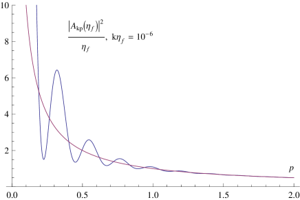
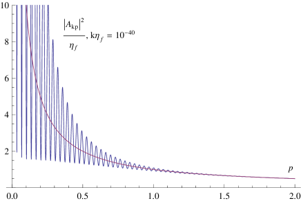
Figure 5: The amplitude of the modes vs. $p$ for two different scales during the inflationary period in the hypersurface. We can see that the modes collapse to $p^{-1}$ for $p>>2/\pi$.

In the figure (5) we show the amplitude of the modes in the effective 4D hypersurface versus $p$ for two different wavenumbers $k$, during the inflationary epoch. The amplitude is not divergent for $p\rightarrow 0$, since in this limit case we have $(\tanh p)_{{p\rightarrow 0}}\rightarrow p$, $(\cosh p)_{p\rightarrow 0}\rightarrow 1$ and $(\sinh p)_{p\rightarrow 0}\rightarrow p$, so that

$${\cal A}_{k0}{\cal A}_{k0}^{\ast}|_{IR}\simeq\frac{\pi\eta}{2}\left[1+\frac{4}{\pi^{2}}\left[\ln\left(\frac{k\eta}{2}\right)-\gamma\right]^{2}\right],$$ (43)

where $\gamma\simeq 0.5772..$ is the Euler constant. On the other hand, when $p\gg 2/\pi$ one obtains $(\tanh p)_{p\gg 2/\pi}\rightarrow 1$, while the quadratic sines and cosines have the same argument reducing to unity. Finally, we obtain

$${\cal A}_{kp\gg 2/\pi}{\cal A}_{kp\gg 2/\pi}^{\ast}|_{IR}\simeq\frac{\eta}{p}=\frac{a^{-1}}{pH_{0}}.$$ (44)

Other important quantity is the amplitude of temporal derivatives of the modes. In the long wavelength limit it takes the form

$${\cal A}^{\prime}_{kp}{\cal A}_{kp}^{{}^{\prime}\ast}|_{IR}\simeq\frac{4p}{\eta}\left[\tanh\left(\frac{p\pi}{2}\right)\sin^{2}\left[p\ln\left(\frac{k\eta}{2}\right)-\gamma_{p}\right]+\frac{\cos^{2}\left[p\ln\left(\frac{k\eta}{2}\right)-\gamma_{p}\right]}{\tanh\left(\frac{p\pi}{2}\right)}\right].$$ (45)

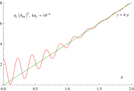
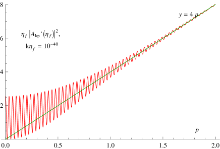
Figure 6: Amplitude of the derivatives of the modes for two scales. The asymptotic value is $4p$

In the figure (6) we show the amplitude of the derivatives of the modes for two different wavenumbers $k$. When $p=0$, we obtain

$${\cal A}^{\prime}_{k0}{\cal A}_{k0}^{{}^{\prime}\ast}|_{IR}\simeq\frac{8}{\pi\eta}=\frac{8H_{0}}{\pi}a(\eta),$$ (46)

while for $p\gg 2/\pi$, we get

$${\cal A}^{\prime}_{kp}{\cal A}_{kp}^{{}^{\prime}\ast}|_{IR}\simeq\frac{4p}{\eta}=4pH_{0}\,a(\eta),$$ (47)

so that in both limits grows as $H_{0}\,a(\eta)$.

IV Electrodynamics on a 4D hypersurface

With the aim to study the effective 4D dynamics of the fields without propagation in a de Sitter spacetime, we shall consider a static foliation $w=w_{0}$ on the metric (5). This hypersurface is relevant to describe a de Sitter expansion of the universe in the early inflationary epoch.

IV.1 Effective 4D quantization

Once we make the foliation on the fifth coordinate $w=w_{0}$ and the modes are quantized [see appendix (B)], we obtain the modes ${\cal A}_{km}(\eta)\equiv b(w)\,a(\eta){A}_{km}(\eta)$ that yield the equations of motion (17)

$$\frac{d^{2}{\cal A}_{km}}{d\eta^{2}}+\left[k^{2}-\frac{m(m+1)}{\eta^{2}}\right]{\cal A}_{km}=0,$$ (48)

which comply with the normalization condition

$$b^{2}\,a^{2}\,W[A_{km}(\eta)]=i,$$ (49)

that is compatible with the commutation relationships (132).

IV.2 Inflaton modes on 4D

Once fixed the Coulomb Gauge, and with our ansatz (11), there is only one possible solution for the extra component $A_{4}$: the one with the value $m=-1$. We call this solution as $\phi_{k}$, that behaves as a massless scalar field in 4D. Using the equation (48) we obtain the general solution

$$\phi_{k}(\eta,w)=b^{-1}(k\eta)^{3/2}\left[c_{1}{\cal H}_{\frac{3}{2}}^{(1)}(k\eta)+c_{2}{\cal H}_{\frac{3}{2}}^{(2)}(k\eta)\right].$$ (50)

From the condition (49) we can set one constant to zero $c_{2}=0$, so that $c_{1}(k)=\sqrt{\frac{H_{0}^{2}}{\pi k^{3}}}$. In the infrared limit we obtain

$$\left.\phi_{k}\right|_{IR}=\frac{H_{0}}{\pi b}\left[\frac{4}{9}k^{\frac{3}{2}}\eta^{3}+i\frac{3}{2}k^{-\frac{3}{2}}\right].$$ (51)

This spectrum is exactly scale invariant, something we would expect because we are dealing with 4D hypersurfaces $w=0$ that suffer a de Sitter expansion. In this case the amplitude of the modes, $|\phi_{k}|\equiv\sqrt{\phi_{k}\phi^{*}_{k}}$, is constant

$$|\phi_{k}|\simeq\frac{3H_{0}}{2\pi b}k^{-\frac{3}{2}},$$ (52)

in agreement with what one expects in a de Sitter expansion for a massless scalar field. In this sense this special solution has the appropriate spectrum of the inflaton fluctuations.

IV.3 Vector modes confined to the 4D hypersurface

Lets turn to study fields where their modes are confined to propagate in the effective 4D hypersurface, which describes a de Sitter expansion for the universe. We proposed an ansatz for such fields as ${A^{C}}(\eta,\mathbf{R},w)=e^{mH_{0}w}{A}_{m}^{C}(\eta,\mathbf{R})$, depending exponentially in a parameter $m\in\mathbb{R}$. This choice, however, can be problematic when the parameter $m<0$. In this case the fluctuations blow when $w\rightarrow-\infty$. In the same way, if $m>0$ the fluctuations blow as $w\rightarrow\infty$. To avoid this problem we can suppose that these fluctuations reach a maximum in the 4D hypersurface, and therefore decay exponentially at both sides. A possible symmetry to choose is $\mathbb{Z}_{2}$, common in brane theories. In this sense, for example, if $m<0$, we have the solution $e^{-mH_{0}w}$ for $w<0$. However, the solution will be $e^{mH_{0}w}$ for $w>0$. In this way the function is continuous in $w=0$, but not its derivative that suffers a discontinuity $2mH_{0}$. Apart from this, it appears a complication since the equations of motion (48) change when we go from one side to the other of the hypersurface. This is due to the fact they are not invariant under the transformation $m\leftrightarrow-m$. A closer inspection shows us that they are invariant under the change $m\leftrightarrow-(m+1)$. This means that the $m$-mode is equivalent to the $-(m+1)$-mode. Then, we use the solution $e^{-(m+1)H_{0}w}$ when $m<-1$ for the interval $w<0$ and $e^{mH_{0}w}$ for the interval $w>0$. On the other hand, when $m>0$ the solutions should be $e^{mH_{0}w}$ for $w<0$ and $e^{-(m+1)H_{0}w}$ for $w>0$. This idea is sketched in the figure (1). In the interval $-1<m<0$ we don’t have this symmetry and the solutions would irremediable blow. For this reason they remain excluded.

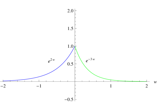
Figure 1: Dependence of the modes outside the effective 4D hypersurface using the shift symmetry $m\leftrightarrow-(m+1)$

The solution written in terms of Bessel functions, reads

$${\cal A}_{km}(\eta)=(k\eta)^{\frac{1}{2}}\left[{c_{1}}_{(k,m)}J_{\frac{1}{2}+m}(k\eta)+{c_{2}}_{(k,m)}J_{-\frac{1}{2}-m}(k\eta)\right].$$ (53)

The quantum limit of this modes is

$${\cal A}_{km}|_{UV}\longrightarrow\frac{1}{\sqrt{2k}}e^{-ik\eta},\hskip 28.45274ptk\eta\longrightarrow-\infty.$$ (54)

Using the normalization condition and the asymptotic form of the Bessel functions we find

$${c_{1}}_{(k,m)} = -{c_{2}}_{(k,m)}e^{-i\pi\left(\frac{1}{2}+m\right)},$$ (55)

$${c_{2}}_{(k,m)} = \sqrt{\frac{\pi}{4k}}\frac{e^{-i\pi\frac{(1-m)}{2}}}{\cos(m\pi)}.$$ (56)

Once defined the modes for all scales we can find their large scale limit for $(k\eta\rightarrow 0)$

$${\cal A}_{km}(\eta)|_{IR} = \frac{\sqrt{\pi}}{2^{\frac{1}{2}-m}}\frac{e^{-i\pi\frac{m}{2}}}{\Gamma\left(\frac{1}{2}-m\right)\cos(m\pi)}k^{-\frac{1}{2}}(k\eta)^{-m}+$$ (57)

$$+ \frac{\sqrt{\pi}}{2^{\frac{3}{2}+m}}\frac{e^{i\pi\frac{(m+1)}{2}}}{\Gamma\left(\frac{3}{2}+m\right)\cos((m+1)\pi)}k^{-\frac{1}{2}}(k\eta)^{m+1}.$$ (58)

This is the long wavelength solution for the modes $m<-1$ when $w>0$. It is also the solution for $m>0$ when $w<0$. It is interesting that the solutions do not change when we transform $-m\leftrightarrow(m+1)$, in this case the first term shifts to the second and the second to the first. It is useful to introduce the following dimensionless function 2008JCAP…01..025M to calculate the amplitude of the modes.

$${\cal F}(\mu)\equiv\frac{\pi}{2^{2\mu+1}\Gamma^{2}{(\frac{1}{2}+\mu)}\cos^{2}(\mu\pi)},$$ (59)

where

$$\mu=-m,\ \ m>-\frac{1}{2}\hskip 28.45274pt\hskip 28.45274pt\mu=m+1,\ \ m<-\frac{1}{2}.$$ (60)

The function only diverges in $\mu=-1/2$, dividing the function in two well behaved branches. Previously we noted that only the modes with $m\leq-1$ and $m\geq 0$ have the symmetry to avoid divergences and infinities. This means that for this modes the function is well behaved.

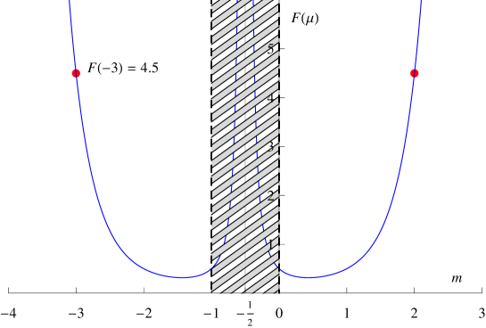
Figure 2: The amplitude ${\cal F}(m)$ for modes without propagation outside the hypersurface. The invariant spectrum for magnetic fields will be achieved for $m=-3$. The dashed sector is forbidden so the fields are fluctuations that do not diverge in the extra coordinates infinities.

The amplitude of the modes in the hypersurface $w=0$ is

$$\hat{{\cal A}}_{k\mu}(\eta)\hat{{\cal A}}_{k\mu}^{\ast}(\eta)|_{IR}\simeq k^{-1}{\cal F}(\mu)(k\eta)^{2\mu}.$$ (61)

Another useful quantity is the temporal derivative of the modes ${\cal A}_{km}$. We find from (57)

$${\cal A}_{km}^{\prime}(\eta)\simeq\sqrt{\pi}k^{\frac{1}{2}}\left[\frac{e^{-i\frac{m\pi}{2}}(-m)}{2^{\frac{1}{2}-m}\Gamma\left(\frac{1}{2}-m\right)\cos(\pi m)}(k\eta)^{-(m+1)}+\frac{e^{i\frac{\pi(m+1)}{2}}(m+1)}{2^{\frac{3}{2}+m}\Gamma\left(\frac{3}{2}+m\right)\cos(\pi(m+1))}(k\eta)^{m}\right].$$ (62)

Again we define a dimensionless function to describe the amplitude of the modes

$${\cal G}(\theta)\equiv\frac{\pi(\theta+1)^{2}}{2^{3+2\theta}\,\Gamma^{2}\left(\frac{3}{2}+\theta\right)\,\cos^{2}(\pi(\theta+1))},$$ (63)

where $\theta$ depends of $m$ in the following way

$$\theta=-(m+1),\ \ m>-\frac{1}{2}\hskip 28.45274pt\hskip 28.45274pt\theta=m,\ \ m<-\frac{1}{2}.$$ (64)

The amplitude reads

$${\cal A}_{k\theta}^{\prime}{\cal A}_{k\theta}^{\prime\ast}\simeq k{\cal G}(\theta)(k\eta)^{2\theta}.$$ (65)

V Electromagnetic energy densities

The stress tensor we find from the action is

$$T_{AB}=-g^{CD}F_{AC}F_{DB}-\frac{1}{4}g_{AB}g^{CD}g^{EF}F_{DF}F_{CE}.$$ (66)

In the same way as in the usual 4D Maxwell theory, where $T_{00}=-(E^{2}+B^{2})$, we can introduce an expression for the temporal-temporal component of the stress tensor as the sum of the individual energies of each physical field

$$T_{00}=T_{00}^{E_{i}}+T_{00}^{B_{i}}+T_{00}^{E_{4}}+T_{00}^{B_{ij}}.$$ (67)

Lets write explicitly each of the previous contributions to the energy density as seen by a 4D comoving observer. The vector magnetic part of it, is

$${T^{(B_{i})}}_{00}=-\frac{g_{00}}{2}g^{ij}g^{kl}F_{jl}.$$ (68)

Since $B_{4i}B^{4i}=g^{44}B_{i}B^{i}$ and $B_{i}=\epsilon_{ijk}a^{-1}\partial_{j}A_{k}$, we get

$$B_{4i}B^{4i}=b^{-4}a^{-4}\left[\partial_{j}A_{k}\partial_{j}A_{k}-\partial_{j}A_{k}\partial_{k}A_{j}\right],$$ (69)

so that

$${T^{(B_{i})}}_{00}=-\frac{b^{2}a^{2}}{2}B_{4i}B^{4i}=\frac{1}{2}a^{2}B_{i}B^{i}.$$ (70)

This is the same result that obtained with the usual 4D electrodynamics. The contribution due to the electric field (vector) part is

$${T^{(E_{i})}}_{00}=\frac{1}{2}g^{ij}F_{0i}F_{0j}=\frac{b^{2}a^{2}}{2}E_{i}\,E^{i},$$ (71)

and the electric (scalar) part

$${T^{(E_{4})}}_{00}=\frac{b^{2}\,a^{2}}{2}E_{4}E^{4}.$$ (72)

Finally, the contribution due to the tensor magnetic part is

$${T^{(B_{ij})}}_{00}=-\frac{b^{2}a^{2}}{2}B_{ij}B^{ij}.$$ (73)

The energy density is defined as $\rho\equiv-\langle{T}_{0}^{0}\rangle$. In our coordinates it takes the form

$$\rho=\frac{1}{2}\left\langle-E_{i}E^{i}-E_{4}E^{4}+B_{4i}B^{4i}+B_{ij}B^{ij}\right\rangle.$$ (74)

All the terms are positive, $E_{i}E^{i}=-b^{-2}a^{-2}E_{i}^{2}$ and $E_{4}E^{4}=-b^{-2}E_{4}^{2}$ [in comoving coordinates (5)]. The previous result in any coordinate system reads

$$\rho=\frac{1}{2}\left\langle-E_{A}E^{A}+B_{CD}B^{CD}\right\rangle.$$ (75)

V.1 Energy density due to Magnetic vector $B_{i}$

We can calculate the contribution of the magnetic vector to energy density defined as $\rho_{(B_{i})}\equiv-\langle{T^{(B_{i})}}_{0}^{0}\rangle$:

$$\langle{T^{(B_{i})}}_{0}^{0}\rangle=-\frac{1}{2}\langle{B_{4i}B^{4i}}\rangle.$$ (76)

Using the expansion in the modes $A_{kp}$, we obtain its derivative in the direction $j_{1}$

$$\partial_{j_{1}}A_{j_{2}}=e^{-\frac{H_{0}w}{2}}\int\frac{d^{3}k}{(2\pi)^{\frac{3}{2}}}\frac{dp}{(2\pi)^{\frac{1}{2}}}\sum_{\lambda=1}^{2}\epsilon_{\lambda j_{2}}\left((ik_{j_{1}})b_{\lambda}e^{i(\mathbf{k}\cdot\mathbf{R}+ipH_{0}w)}A_{kp}+(-ik_{j_{1}})b_{\lambda}e^{-i(\mathbf{k}\cdot\mathbf{R}+ipH_{0}w)}A^{\ast}_{kp}\right).$$ (77)

Its vacuum expectation value is given by

$$\langle 0|\partial_{j_{1}}A_{j_{2}}\partial_{j_{3}}A_{j_{4}}|0\rangle=e^{-H_{0}w}\int\frac{d^{3}k}{(2\pi)^{\frac{3}{2}}}\frac{dp}{(2\pi)^{\frac{1}{2}}}|A_{kp}|^{2}\sum_{\lambda=1}^{2}k_{j_{1}}k_{j_{3}}\epsilon_{\lambda j_{2}}\epsilon_{\lambda j_{4}}.$$ (78)

So that $\langle{T^{(B_{i})}}_{0}^{0}\rangle$ can be written as

$$\langle{T^{(B_{i})}}_{0}^{0}\rangle = -\frac{1}{2\,b^{5}a^{4}}\int\frac{d^{3}k}{(2\pi)^{3}}\frac{dp}{2\pi}A_{kp}A_{kp}^{\ast}$$ (79)

$$\times\sum_{\lambda=1}^{2}\left(k_{j}k_{j}\epsilon_{i\lambda}\epsilon_{i\lambda}-k_{i}\epsilon_{i\lambda}k_{j}\epsilon_{j\lambda}\right).$$

Using the completeness relation projected to the 3D space and the transversal condition $k_{i}\vec{\epsilon_{i\lambda}}=0$, the second term in the previous expression vanishes, while the first one holds

$$\sum_{\lambda=1}^{2}\left(k_{j}k_{j}\epsilon_{i\lambda}\epsilon_{i\lambda}-k_{i}\epsilon_{i\lambda}k_{j}\epsilon_{j\lambda}\right)=2k^{2}b^{2}a^{2}.$$ (80)

Since the solution depends on the absolute value of $p$, we can write the integral as $\int_{-\infty}^{\infty}dp=2\int_{0}^{\infty}dp$, so that the magnetic contribution to the energy density is

$$\rho_{(B_{i})} = \frac{1}{2\pi^{2}b^{3}}\int_{0}^{\infty}\frac{dk}{k}\frac{dp}{\pi}k^{5}\left|\frac{A_{kp}}{a}\right|^{2}$$ (81)

$$= \frac{1}{2\pi^{2}b^{5}}\int_{0}^{\infty}\frac{dk}{k}\frac{dp}{\pi}k^{5}\frac{|{\cal A}_{kp}|^{2}}{a^{4}}.$$

The energy density stored at a certain scale $k$ for unity of $p$ is

$$\frac{d}{dkdp}\rho_{(B_{i})}(\eta,k.p)=\frac{1}{2\pi^{3}}\frac{k^{4}}{b^{5}a^{4}}\left|{\cal A}_{kp}\right|^{2}.$$ (82)

Recalling (42) we arrive to

$$\frac{d}{dkdp}\rho_{(B_{i})}(\eta,k,p)=\frac{1}{2\pi^{3}}\frac{k^{4}}{pH_{0}b^{5}a^{5}}\left[\tanh\left(\frac{p\pi}{2}\right)\cos^{2}\left[p\ln\left(\frac{k\eta}{2}\right)-\gamma_{p}\right]+\frac{\sin^{2}\left[p\ln\left(\frac{k\eta}{2}\right)-\gamma_{p}\right]}{\tanh\left(\frac{p\pi}{2}\right)}\right].$$ (83)

The $k$-dependence of the energy density results of the integration of $\frac{d}{dkdp}\rho_{(B_{i})}(\eta,k,p)$ with respect to $p$. It is not possible to extend to infinite values of $p$ when we perform the integration, this is because there is a certain scale $p_{0}$ for which the modes don’t have a quantum limit. This can be seen from the mode equation (35), where the frequency is time dependent

$$\omega^{2}_{kp}(\eta)=\frac{\frac{1}{4}+p^{2}}{\eta^{2}}+k^{2}.$$ (84)

This frequency is always positive, so the solutions oscillate, but depending on the relative magnitudes between $p$ and the physical wavenumber $k_{phys}=k\,e^{-H_{0}t}$, with respect to which of them oscillates.

In the previous asymptotic limits we have supposed that for modes in the ultraviolet sector, and at the beginning of inflation $t=t_{i}$, we have $k_{phys}(t_{i})\gg H_{0}\sqrt{\frac{1}{4}+p^{2}}$ so $\omega_{kp}(t_{i})\simeq k_{phys}(t_{i})$. But, when inflation ends at $t=t_{f}$, an interval of these wavelengths can increase such that $k_{phys}(t_{f})\ll p$ and then $\omega_{kp}(t_{f})\simeq\sqrt{1/4+p^{2}}$. This means that the actual scales of the observed universe $\lambda_{phys}$ will imply a cut $p_{0}$ in the integral. The rest of the modes with $p>p_{0}$ do not have a quantum origin at the start of inflation.

The connection of inflationary scales to the actual large scales is something uncertain. It is known, approximately, the minimum number of e-folds to solve the problems of planarity of the Big-Bang, but this value depends strongly on the theoretical model. Furthermore, during reheating there exists an important re-scaling of the cosmological lengths 2006Martin .

A physical scale today at $t=t_{h}$, $\lambda^{h}_{phys}$ corresponds to one at the start of inflation by $\lambda^{h}_{phys}=\lambda^{i}_{phys}\frac{a_{h}}{a_{i}}$. In our case we are dealing with a inflationary de Sitter expansion, where $\frac{a_{f}}{a_{i}}=e^{N}$, such that the scales at the end of inflation relate to the actual ones as

$$\frac{a_{h}}{a_{f}}=\frac{\sqrt{8\pi}}{R}\left[\frac{{\rho}_{inf}^{2}}{\Omega_{rad}^{h}\rho^{h}_{cri}}\right]^{1/4},$$ (85)

the Hubble parameter today is $H_{h}\simeq 2.1h\times 10^{-42}GeV$, the cosmological radiation density parameter today is $\Omega^{h}_{rad}\simeq h^{-2}4.3\times 10^{-5}$ Turner , and the parameter $R$ that describes a phase of reheating 2006Martin is in units of $m_{pl}$. It doesn’t exist in the literature a model in the framework of the Induced Matter theories that studies a realistic transition between an inflationary period induced from a 5D vacua and a localized brane dominated by radiation. We then assume that this transition is instantaneous. In our model we obtain a vacuum energy density induced in the hypersurface

$$\rho_{inf}=\frac{3}{\kappa_{5}\psi_{0}^{2}}=\frac{3H_{0}^{2}}{\kappa_{5}}.$$

The critical energy density today is

$$\rho_{cri}=\frac{3H_{h}^{2}m_{pl}^{2}}{8\pi}.$$

The parameter $R$ can be expressed as (for instantaneous reheating)

$$\ln R=\frac{1}{4}\ln\rho_{inf},$$

obtaining the following relation

$$\frac{a_{h}}{a_{f}}=\left(\frac{\rho_{inf}}{\Omega_{rad}^{h}\rho^{h}_{cri}}\right)^{1/4}.$$ (86)

If we use the condition $k_{phys}(t_{i})\gg H_{0}\sqrt{\frac{1}{4}+p^{2}}$ we can estimate a cut for the values of $p$, so we are keeping modes with quantum initial conditions

$$p_{0}\ll\sqrt{\left[\frac{e^{2N}}{(\lambda^{h}_{phys})^{2}H_{0}H_{h}\sqrt{\Omega^{h}_{rad}}}\right]-\frac{1}{4}}.$$ (87)

There are three uncertainties in the last relation, the scale of inflation $H_{0}/m_{pl}$ , the amount of inflation $N$ and the scales of coherence of the cosmological magnetic field. Slight variations in this parameters affect significatively the cut $p_{0}$. In table 1 we give some examples on how these parameters $N$, $H_{0}$ y $\lambda^{h}_{phys}$ restrict $p_{0}$.

$N$	$H_{0}$($m_{pl}$)	$\lambda^{h}_{phys}$(Mpc)	$p_{0}\ll$
50	$10^{-9}$	$10^{4}$	$-$
60	$10^{-9}$	$10^{4}$	$45$
65	$10^{-9}$	$10^{4}$	$6.7\times 10^{3}$
50	$10^{-6}$	$10^{4}$	$-$
60	$10^{-6}$	$10^{4}$	$1.34$
65	$10^{-6}$	$10^{4}$	$2.1\times 10^{2}$
50	$10^{-9}$	$10^{2}$	$-$
60	$10^{-9}$	$10^{2}$	$4.5\times 10^{3}$
65	$10^{-9}$	$10^{2}$	$6.7\times 10^{5}$
50	$10^{-6}$	$10^{2}$	$-$
60	$10^{-6}$	$10^{2}$	$1.4\times 10^{2}$
65	$10^{-6}$	$10^{2}$	$2.1\times 10^{5}$

Table 1: we show some relevant examples on how the parameters $N$, $H_{0}$ y $\lambda^{h}_{phys}$ restrict $p_{0}$.

Using some numerical calculations [the reader can see the appendix (D)], we can compute the magnetic energy density at a certain scale $k$, for the modes that propagate on the extra coordinate $\frac{d}{dk}\rho_{(B_{i})}(\eta,k,p_{0})\equiv\int_{0}^{p_{0}}dp\frac{d}{dkdp}\rho_{(B_{i})}(\eta,k,p)$ with

$$\frac{d}{dk}\rho_{(B_{i})}(\eta,k,p_{0})\simeq\frac{1}{2\pi^{3}}\frac{k^{4}}{H_{0}b^{5}a^{5}}\ln\left(e^{1.303}\frac{p_{0}\pi}{8}\frac{k}{H_{0}\,a}\right),$$ (88)

where $p_{0}>4/\pi$. From the figure (3) we see that for reasonable amounts of inflation, $N=60$, all of the relevant scales are produced. However, for a lower value of e-folds, $N=55$, and with a scale of inflation $H_{0}/m_{pl}\sim 10^{-6}$ there are excluded the modes corresponding with scales larger than $100\,Mpc$.

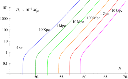
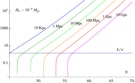
Figure 3: The cut $p_{0}$ vs. the amount of inflation $N$ for small proto-galactic scales of $10Kpc$ to very large scales of the observable universe $10Gpc$. We have plotted two sub-Planckian scales, in the left: $H_{0}\sim 10^{-6}m_{planck}=10^{13}GeV$, and in the right $H_{0}\sim 10^{-9}m_{planck}$. It is important to notice the change in the behavior of the cut at $4/\pi$

For the modes ${\cal A}_{km}(\eta)$ we must compute

$$\rho_{(B_{i})} = \frac{1}{2\pi^{2}}\int_{0}^{\infty}\frac{dk}{k}\frac{k^{5}}{b^{5}}\left|\frac{A_{km}}{a}\right|^{2}$$ (89)

$$= \frac{1}{2\pi^{2}}\int_{0}^{\infty}\frac{dk}{k}\frac{k^{5}}{b^{5}}\frac{|{\cal A}_{km}|^{2}}{a^{4}}.$$

The energy density at a certain scale $k$, is

$$\frac{d}{dln(k)}\rho_{(B_{i})}(\eta,k)=\frac{1}{2\pi^{3}}\frac{k^{5}}{b^{5}\,a^{4}}\left|{\cal A}_{km}\right|^{2}.$$ (90)

Recalling the amplitude (61), we get

$$\frac{d}{dln(k)}\rho_{(B_{i})}(\eta,k)=\frac{1}{2\pi^{2}}\frac{k^{4}}{b^{5}a^{4}}{\cal F}(\mu)(k\eta)^{2\mu}.$$ (91)

This also was obtained in 2008JCAP…01..025M , but in other context.

V.2 Energy density due to the magnetic tensor $B_{ij}$

The energy density that come from magnetic tensor is given by $\rho_{(B_{ij})}=-\langle{T^{(B_{ij})}}_{0}^{0}\rangle$

$$\rho_{(B_{ij})}=\frac{1}{2}\langle B_{ij}B^{ij}\rangle=\frac{1}{2\pi^{3}}\int dkdp\frac{k^{2}}{b^{5}a^{2}}\left(\frac{1}{4}+p^{2}\right)H_{0}^{2}|{\cal A}_{kp}|^{2},$$ (92)

from $\frac{d}{dk}\rho_{(B_{ij})}(\eta,k,p_{0})\equiv\int_{0}^{p_{0}}dp\frac{d}{dkdp}\rho_{(B_{ij})}(\eta,k,p)$ we obtain

$$\frac{d}{dk}\rho_{(B_{ij})}\left(\eta,k,p_{0}\right)\simeq\frac{1}{2\pi^{3}}\frac{k^{2}H_{0}}{b^{5}a^{3}}\left[\frac{1}{4}\ln\left(e^{1.21}\frac{p_{0}\pi}{8}\frac{k}{H_{0}a}\right)+\frac{p_{0}^{2}}{2}-\frac{8}{\pi^{2}}\right],$$ (93)

where $p_{0}>4/\pi$.

From the modes ${\cal A}_{km}$ it is easy to see that

$$\frac{d}{dln(k)}\rho_{(B_{ij})}(\eta,k,\mu)=\frac{1}{2\pi^{2}}\mu^{2}H_{0}^{2}{\cal F}(\mu)\frac{k^{2}}{b^{5}a^{2}}(k\eta)^{2\mu}.$$ (94)

If $m=-1$ we also have a contribution from the scalar field $\phi_{k}$ in (52) and after considering that ${\cal F}(-1)=1/2$, we obtain

$$\frac{d}{dln(k)}\rho_{(B_{ij})}\left(\eta,k,m=-1\right)=\frac{13H_{0}^{2}}{8\pi^{2}b^{5}}\frac{k^{2}}{a^{2}}.$$ (95)

V.3 Energy density due to the Electric vector $E_{i}$

The energy density related to the electric field $E_{i}$ it is

$$\rho_{(E_{i})}=-\langle{T^{(E_{i})}}_{0}^{0}\rangle = \frac{1}{2a^{4}b^{4}}\langle\partial_{0}A_{i}\partial_{0}A_{i}\rangle,$$ (96)

$$= \frac{1}{4\pi^{2}a^{4}b^{5}}\int dk\frac{dp}{\pi}k^{2}|{\cal A}_{kp}^{\prime}|^{2}.$$

Calculating $\frac{d}{dk}\rho_{(E_{i})}(\eta,k,p_{0})\equiv\int_{0}^{p_{0}}dp\frac{d}{dkdp}\rho_{(E_{i})}(\eta,k,p)$ we get

$$\frac{d}{dln(k)}\rho_{(E_{i})}(\eta,k,p_{0})\simeq\frac{1}{\pi^{3}}\frac{k^{3}H_{0}}{b^{5}a^{3}}\left[2.77+\frac{p_{0}^{2}}{2}\right],$$ (97)

with $p_{0}>4/\pi$.

The energy density associated to the modes ${\cal A}_{km}$ is

$$\rho_{(E_{i})}=\frac{1}{4\pi^{2}b^{5}a^{4}}\int dkk^{2}|{\cal A}_{km}^{\prime}|^{2}$$ (98)

where we identify the energy density stored at a certain scale $k$ as

$$\frac{d\rho_{(E_{i})}}{dln(k)}=\frac{1}{4\pi^{2}}\frac{k^{4}}{b^{5}a^{4}}{\cal G}(\theta)(k\eta)^{2\theta}.$$ (99)

this is the same result derived in 2008JCAP…01..025M .

V.4 Energy density due to the Electric scalar $E_{4}$

The energy density corresponding to the scalar electric field is $\rho_{(E_{4})}=-\langle{T^{(E_{4})}}^{0}_{0}\rangle$, so that

$$\rho_{(E_{4})} = \frac{1}{2b^{2}a^{4}}\langle\partial_{0}A_{4}\partial_{0}A_{4}\rangle,$$ (100)

$$= \frac{1}{2b^{3}}\int\frac{dk}{2\pi^{2}}k^{2}\left|\frac{\phi_{k}^{\prime}}{a}\right|^{2},$$

$$= \int\frac{dk}{k}\frac{d\rho_{(E_{4})}}{dln(k)},$$

the energy density at a given scale $k$, is

$$\frac{d\rho_{(E_{4})}}{dln(k)}=\frac{1}{(9\pi^{2}H_{0})^{2}}\frac{k^{6}}{b^{5}a^{6}}.$$ (101)

this component decays strongly with the expansion. It is important to notice that this contribution only appear when we are considering a field that doesn’t propagate in the extra dimension and has a exponential decay in $w$ with $m=-1$.

V.5 Spectrum of the fields

In table 2 we summarize the spectrums of the 5D electromagnetic fields for the two types of fields studied

Power spectrum	5D	$n$	4D	$m<-\frac{1}{2}$	$m>-\frac{1}{2}$	$\mu$	$n$
$2\pi^{2}H_{0}^{-4}\frac{d}{\ln k}\rho_{(B)}$	$x^{5}\ln\left(e^{1.303}\frac{p_{0}\pi}{8}x\right)$	$\sim 5$		${\cal F}(m+1)x^{6+2m}$	${\cal F}(-m)x^{4-2m}$	${\cal F}(\mu)x^{4+2\mu}$	$4+2\mu$
$2\pi^{2}H_{0}^{-4}\frac{d}{\ln k}\rho_{B_{ij}}$	$x^{3}\ln\left(e^{1.21}\frac{p_{0}\pi}{8}x\right)$	$\sim 3$		$(m+1)^{2}{\cal F}(m+1)x^{4+2m}$	$m^{2}{\cal F}(-m)x^{2-2m}$	$\mu^{2}{\cal F}(\mu)x^{2+2\mu}$	$2+2\mu$
$2\pi^{2}H_{0}^{-4}\frac{d}{\ln k}\rho_{E_{i}}$	$x^{3}\left(2.77+\frac{p_{0}^{2}}{2}\right)$	$\sim 3$		${\cal G}(m)x^{4+2m}$	${\cal G}(-m-1)x^{2-2m}$	${\cal G}(\theta)x^{4+2\theta}$	$4+2\theta$
$9\pi^{2}H_{0}^{-4}\frac{d}{\ln k}\rho_{E_{4}}$	—	—	$m=-1$	$x^{6}$	—	—	$6$

Table 2: The spectral indexes of the fields that can propagate in the extra dimension are approximate, since there is a logarithmic factor and so it doesn’t strictly obey a power law. This expressions for the energy density are very blue tilted, so they decay to residual values at the end of inflation. The only solutions that can give significant seeds for galactic magnetic fields are does arising from real values of $m$. In particular, when $m=-3$ we obtain an invariant spectrum for the vector magnetic fields. For this value the vector electric and the tensor magnetic fields are red tilted $n=-2$. For the fields with $m=-2$, the electric and tensor magnetic fields are scale invariant, but the vector magnetic fields is blue tilted with $n_{B}=2$.

VI Back-reaction effects

In order to make an analysis of the back-reaction effects we shall estimate the energy density due to $B_{ij}$ and the electric (vector) field, which could be more problematic because, in both cases their energy densities evolve as $(k\eta)^{-2}$. In order to back-reaction effects to be negligible at the end of inflation, we shall require that these energy densities to be smaller than the critical background energy density: $\rho_{crit}=3H_{0}^{2}m_{pl}^{2}/(8\pi)$.

From the condition $\frac{d}{dln(k)}\rho_{(B_{ij})}<\rho_{crit}$ in the eq. (94), we obtain that

$$\left(\frac{k}{a}\right)^{2(1+\mu)}<\frac{3(H_{0}/m_{pl})^{2\mu}}{4{\cal F}(\mu)\mu^{2}}m_{pl}^{2(1+\mu)}.$$ (102)

If we consider $\mu<-1$, modes for which back-reaction effects are negligible has physical wavelengths of the order

$$\left.\lambda_{phys}\right|_{B_{ij}}<\left[\frac{4\mu^{2}{\cal F}(\mu)}{3}\right]^{\frac{1}{2(1+\mu)}}\left(\frac{H_{0}}{m_{pl}}\right)^{\frac{1}{1+\mu}}\,\lambda_{H}.$$ (103)

In order to make an estimation we can consider a scale invariant magnetic spectrum with $\mu=-2$ and a Hubble parameter $H_{0}=1.0\times 10^{-5}\,m_{pl}$. In this case we obtain that the

$$\left.\lambda_{phys}\right|_{B_{ij}}<0.204\times 10^{5}\,\lambda_{H},$$ (104)

where $\lambda_{H}=1/H_{0}$ is the wavelength related to the Hubble radius during inflation (we are considering $c=1$.

On the other hand, from the eq. (99), we obtain that the condition to back reaction effects do not be relevant in the background evolution of the universe, is (for cases with $\theta<-2$)

$$\left.\lambda_{phys}\right|_{E_{i}}<\left[\frac{2{\cal G}(\theta)}{3\pi}\right]^{\frac{1}{2(2+\theta)}}\left(\frac{H_{0}}{m_{pl}}\right)^{\frac{1}{2+\theta}}\,\lambda_{H},$$ (105)

that for a scale invariant magnetic spectrum with $\mu=m=-2$, for which $\theta=-3$, results to be

$$\left.\lambda_{phys}\right|_{E_{i}}<0.512\times 10^{5}\,\lambda_{H},$$ (106)

which is bigger than the Hubble horizon during inflation. Hence, in both cases, for $B_{ij}$ end $E_{i}$ the modes with wavelengths which are on cosmological scales today (these wavelengths are larger than the Hubble radius during inflation) are not problematic in the back-reaction sense. On the other hand, it is easy to see that $d\rho_{B_{i}}/[dln(k)]$ is or the order $(H_{0}/m_{pl})^{2}\sim 10^{-10}$ times smaller than the background energy density, so that this contribution is negligible. Of course, in our estimation we are considering a scale invariant spectrum for the magnetic fields, but it can be seen from the figure (8) that (for $H_{0}\simeq 10^{-5}\,m_{pl}$), the admissible spectrums for the magnetic fields has a spectral index $-0.12<n_{B}<0.1$ very close with an scale invariant one. Our results in this sense are in agreement with those obtained in 2008JCAP…01..025M . This topic has been discussed in several articlesa1 ; a2 ; a3 .

VII Seed magnetic fields

We are aimed to compare the present day strength of magnetic fields with the predictions of our theory, we can estimate the actual magnetic fields generated by this model, the magnetic density parameter defined at a scale $L=2\pi/k$ is

$$\Omega_{B}(k)\equiv\frac{\rho_{(B)}(t=t_{h},k)}{\rho_{cri}}.$$ (107)

The energy density related to the magnetic fields after inflation decay adiabatically with the expansion as $a^{-4}$

$$\rho_{(B)}(t=t_{h},k)=\frac{d\rho_{(B)}}{d\ln k}(t=t_{f},k)\left(\frac{a_{f}}{a_{h}}\right)^{4}.$$ (108)

Using the expression (91) for the magnetic density, we obtain

$$\frac{d\Omega_{(B)}}{d\ln k}=\frac{32}{9}{\cal F}(\mu)\left(\frac{\rho_{cri}}{m_{pl}}\right)\left(\frac{\rho_{cri}}{\rho_{inf}}\right)^{\mu}\left(\frac{a_{h}}{a_{f}}\right)^{2\mu}\left(\frac{k}{a_{h}\,H_{h}}\right)^{2\mu+4}.$$ (109)

Replacing the values for $\rho_{cri}$, $\rho_{inf}$ and $(a_{h}/a_{f})$ we may write 2008JCAP…01..025M

$$\frac{d\Omega_{(B)}}{d\ln k}\simeq 2.4\times 10^{-7}(2.28\times 10^{-58})^{\mu+2}{\cal F}(\mu)R^{-2\mu}h^{2\mu+2}\left(\frac{k}{a_{h}\,H_{h}}\right)^{2\mu+4}.$$ (110)

Also, the magnetic density parameter is

$$h^{2}\frac{d\Omega_{(B)}}{d\ln k}\simeq 2.43\times\,10^{6}\left(\frac{B}{Gauss}\right)^{2},$$ (111)

where we use that $1\,Tesla^{2}/2\simeq 1.9\times 10^{-32}\,GeV^{4}$ and $1\,Tesla=10^{4}\,Gauss$. We then arrive to an expression for the seeds of the cosmological magnetic field

$$\left(\frac{B}{Gauss}\right)\simeq\,3.16\times 10^{-7}h^{\mu+2}(2.28\times 10^{-58})^{1+\frac{\mu}{2}}{\cal F}(\mu)^{\frac{1}{2}}R^{-\mu}\left(\frac{k}{a_{h}\,H_{h}}\right)^{\mu+2}.$$ (112)

This is the final expression for magnetic fields generated from the fields ${\cal A}_{km}$. The values of $R$, without considering a particular model of reheating, are constrained with a necessary cut for them to preserve nucleosynthesis:

$$\rho_{inf}>\rho_{nuc}\simeq 10^{-85}m_{pl}^{4}.$$

Furthermore, if inflation holds at sub-Planckian scales we would need that $H_{inf}/m_{pl}<1.3\times 10^{-5}$, see 2006Martin . If additionally we assume an instantaneous transition from reheating to radiation [which is a good approximation on large (cosmological) scales], and keeping in mind that in this case $R^{4}\simeq(3/8\pi)(H_{0}^{2}\,m^{2}_{pl})$, we obtain that

$$-24.7\lesssim\ln R\lesssim-5.71,$$ (113)

which can be written in terms of inflationary scales

$$9\times 10^{-43}<\frac{H_{0}}{m_{pl}}<1.3\times 10^{-5}.$$ (114)

The scale invariant spectrum in (112) is achieved when $m=-3$

$$\left(\frac{B}{Gauss}\right)_{m=-3}\simeq 8.00\times 10^{-8}\left(\frac{H_{0}}{m_{pl}}\right).$$ (115)

The galactic dynamo scenario impose a lower limit for the seed magnetic fields at the moment of the formation of seminal galaxies, $B>10^{-22}Gauss$ (some models may relax to $10^{-30}\,Gauss$). This then implies a constraining for the scale of the inflation

$$\frac{H_{0}}{m_{pl}}>1.25\times 10^{-15}.$$ (116)

These values are reasonable for sub-Planckian models. In particular, for $H_{0}/m_{pl}\sim\,10^{-9}$, we obtain scale invariant cosmological magnetic fields of amplitude

$$\left(\frac{B}{Gauss}\right)_{m=-3}\simeq\,8.00\times 10^{-17},$$ (117)

which is compatible with dynamos mechanisms.

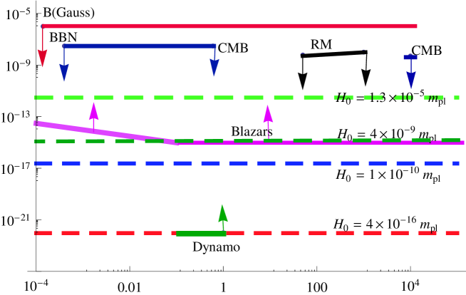
Figure 7: Scale invariant magnetic fields for different inflation scales $H_{0}/m_{pl}$ plotted against cosmic scales in $Mpc$. The upper constraints come from nucleosynthesis, Faraday rotation measures and from the Cosmic Microwave Background. We also include the lower magnetic fields needed to ignite the galactic dynamos and TeV Blazars. For these spectrums the compatible scales are: $4\times 10^{-7}<H_{0}/m_{pl}<1.3\times 10^{-5}$.

In the figure (7) we plotted scale invariant magnetic fields for different inflation scales $H_{0}/m_{pl}$ versus wavelengths expressed in $Mpc$. The upper constraints come from nucleosynthesis, Faraday Rotation measures and from the Cosmic Microwave Background. Furthermore, we include the lower strengths of magnetic fields needed to ignite the galactic dynamos and lower magnetic fields from TeV Blazars observations. Notice that for these spectrums the compatible scales are: $4\,\times\,10^{-7}<H_{0}/m_{pl}<1.3\times 10^{-5}$.

Very recently it was argued a lower bound $B\sim 3\times 10^{-16}$ Gauss on the strength of intergalactic magnetic fields, which stems from the un-observation of GeV gamma-ray emission from electromagnetic cascade initiated by tera-electron volt gamma-ray in an intergalactic medium from Fermi observations in TeV Blazarsnero . More recently, it was argued that these results are in tension with inflationary predictions ponjas . For our model this implies that the minimal scales to produce fields of coherence bigger than $Mpc$ is $H_{0}\simeq 4\times 10^{-9}m_{pl}$. If the coherent fields are to be generated for all scales, including smaller than $Mpc$ then the constraint improves as $L^{-1/2}$ and the scale increases to $4\times 10^{-7}m_{pl}$.

VIII Conclusions

Using some ideas of IMT, we have studied the magnetogenesis produced by a 5D photon field in a hypersurface which undergoes a period of de Sitter inflation. We deduce very blue tilted magnetic fields for photons that can leak outside the 4D hypersurface, with wavenumber $pH_{0}$. In order to produce significative seeds of the magnetic fields to explain actual observations, we need other kind of fields that cannot propagate outside the brane. These fields produce a discontinuity in the stress tensor, so in turn their origin should come from localized sources (i.e., static solutions) on the extra space-like noncompact dimension. We do not study how this fields came from, but once produced we analyze their electromagnetic effects in the 4D effective de Sitter (inflationary) universe. We have found that these fields are candidates to produce relevant magnetogenesis. In particular, they include the invariant scale spectrum for magnetic fields.

An important result here obtained is that we identify new physical electromagnetic fields that arise from the extension of Inflato-electromagnetic Inflationgi ; mb1 ; mb2 , as an extended Maxwell theory. Such fields are, for 4D comoving observes in the hypersurface, a scalar electric field and an antisymmetric magnetic tensor field. This formalism was proposed recently with the aim to describe, in an unified manner, electromagnetic, gravitational and the inflaton fields in the early inflationary universe, from a 5D vacuum. Other conformal symmetry breaking mechanisms have been proposed so fartur . As in our case, most of these are developed in the Coulomb gauge in order to simplify the equations of motion for $A^{\nu}$. In our calculations, the scalar electric field remains very constrained by the actual model, since it is very blue tilted and exists for one specific value of the parameter $m$. In contrast, the magnetic tensor field, $B_{ij}$, and the vector electric components are red tilted with respect to the vector magnetic field. Therefore, its cosmological values at the end of inflation are very important. The electric field is damped during reheating giving its energy to charged particles. The tensor magnetic field should also be extinguished, by transferring its energy to charged particles or transforming to the vector magnetic field. The final fate of this unobserved quantity depends on a model that should explain the transition from this inflationary scenario to the actual universe. However, this issue goes beyond the scope of this paper.

Finally, our results are in very good agreement with recent observationsnero ; if the coherent magnetic fields are to be generated for all scales, including smaller than $Mpc$, magnetic fields with strengths larger than $10^{-15}\,Gauss$ should be generated during inflation on all scales for values of the Hubble parameter larger than $H_{0}>4\times 10^{-7}m_{pl}$, which is very compatible with the accepted values during inflation. In the figure (8) we plotted different admissible spectrums of magnetic fields. Notice that if we take into account the more restrictive constrain that comes from TeV Blazars, we obtain spectrums nearly scale invariants. The most blue tilted compatible spectrum is for $n_{B}\simeq 0.1$ and a scale $H_{0}=1.3\times 10^{-5}m_{pl}$. However, the most red tilted magnetic fields take place for $n_{B}\simeq-0.62$ and a lower scale $H_{0}\sim 10^{-15}m_{pl}$. Therefore, taking into account the observational data the spectral indices for magnetic fields should be in the range $-0.62<n_{B}<0.1$ for $10^{-15}\,m_{pl}<H_{0}<10^{-5}\,m_{pl}$.

Appendix A Conformal coordinates

From (4) with the transformation

$$t=\psi_{0}N,\hskip 28.45274pt\mathbf{R}=\psi_{0}\mathbf{r},\hskip 28.45274pt\psi=\psi,$$ (118)

we obtain the Ponce de Leon metric PdL

$$ds^{2}=\left(\frac{\psi}{\psi_{0}}\right)^{2}\left[dt^{2}-e^{2t/\psi_{0}}d\mathbf{R}^{2}\right]-d\psi^{2}.$$ (119)

The foliations $\psi=\psi_{0}$ yield a 4D de Sitter hypersurface with Hubble parameter $H=\psi_{0}^{-1}$.

The vacuum condition $R_{ab}=0$ is widely satisfied because (119) is Riemann flat. On the other hand, the transport of vectors in the space is not trivial due to the existence of non zero connections. In coordinates (4) the non null connections are

$$\Gamma_{\mu 4}^{\mu}=\psi^{-1},\hskip 28.45274pt\Gamma_{j0}^{i}=\delta_{j}^{i},\hskip 28.45274pt\Gamma_{00}^{4}=\psi,\Gamma_{ij}^{0}=e^{2N}\delta_{j}^{i},\hskip 28.45274pt\Gamma_{ij}^{4}=-\psi e^{2N}\delta_{j}^{i}.$$ (120)

Instead of working with the previous coordinates we will introduce new conformal like coordinates. First we introduce a dimensionless coordinate

$${\cal X}=H_{0}\psi,$$ (121)

yielding

$$ds^{2}=\left(\frac{{\cal X}}{{\cal X}_{0}}\right)^{2}\left[dt^{2}-e^{2H_{0}t/{\cal X}_{0}}d\mathbf{R}^{2}\right]-\frac{d{\cal X}^{2}}{H_{0}^{2}}.$$ (122)

The foliation $\psi=\psi_{0}=H_{0}^{-1}$ corresponds in these coordinates with ${\cal X}={\cal X}_{0}=1$. Now we change to a conformal coordinate

$$\mathfrak{J}=\ln{\cal X},\hskip 28.45274ptd\mathfrak{J}=\frac{d{\cal X}}{{\cal X}}=e^{-\mathfrak{J}}d{\cal X},$$ (123)

such that the metric now reads

$$ds^{2}=e^{2\mathfrak{J}}\left[e^{-\mathfrak{J}_{0}}\left(dt^{2}-e^{2H_{0}e^{-\mathfrak{J}_{0}}t}d\mathbf{R}^{2}\right)-\frac{d\mathfrak{J}^{2}}{H_{0}^{2}}\right].$$ (124)

we can see that taking a constant foliation $\mathfrak{J}=\mathfrak{J}_{1}=cte$, we obtain a 4D de Sitter space with Hubble parameter $H=H_{0}e^{\mathfrak{J}_{1}}$

$$ds^{2}=dT^{2}-e^{2HT}d\mathbf{r}^{2},$$ (125)

where we have defined the cosmic time as $T=e^{\mathfrak{J}_{1}-\mathfrak{J}_{0}}t$. Here we can perceive that the metric (4) and their transformations generate $dS_{4}$-spaces for constant foliations in the extra dimension.

To continue we define the usual conformal time $\eta=\int a(t)^{-1}dt$ with $a(t)=e^{H_{0}e^{-\mathfrak{J}_{0}}t}$. If we define the coordinate $w=H_{0}^{-1}\mathfrak{J}$, the metric finally reads

$$ds^{2}=b(w)^{2}\left[a(\eta)^{2}\left(d\eta^{2}-d\mathbf{R}^{2}\right)-dw^{2}\right],$$ (126)

where the scale factors $b(w)=e^{H_{0}w}$ y $a(\eta)=-\frac{1}{H_{0}\eta}$ are dimensionless. The components of the coordinates $(\eta,\mathbf{R},w)$ have spatial dimensions. The foliation $\psi=\psi_{0}$ corresponds with $w=w_{0}=0$ in these coordinates, such that $b(w_{0})=1$.

Appendix B Mode quantization

In order to obtain the canonical structure of ${}^{(5)}A^{4}_{m}(\eta,\mathbf{R},w_{0})$ and its canonical momentum, we must calculate the effective 4D commutators

$$\left[{}^{(5)}A^{4}_{m}(\eta,\mathbf{R},w_{0}),\pi_{4m^{\prime}}(\eta,\mathbf{R},w_{0})\right] = b^{3}\,a^{2}\left[{}^{(5)}A^{4}_{m}(\eta,\mathbf{R},w_{0}),\frac{\partial}{\partial\eta}{}^{(5)}A^{4}_{m^{\prime}}(\eta,\mathbf{R}^{\prime},w_{0})\right]$$ (127)

$$= i\delta^{(3)}(\mathbf{R}-\mathbf{R}^{\prime})\delta_{mm^{\prime}}b^{(1+m+m^{\prime})}.$$

The quantization follows in the usual way, by expanding in plane waves $e^{i\mathbf{k}\cdot\mathbf{R}}$

$${}^{(5)}A_{4m}(\eta,\mathbf{R},w_{0})=e^{mH_{0}w_{0}}\int\frac{d^{3}k}{(2\pi)^{3/2}}{\epsilon_{4}}_{s=4}\left[a_{\mathbf{k}m}e^{i\mathbf{k}\cdot\mathbf{R}}\phi_{km}(\eta)+a^{\dagger}_{\mathbf{k}m}e^{-i\mathbf{k}\cdot\mathbf{R}}\phi^{\ast}_{km}(\eta)\right].$$ (128)

The creation and annihilation operators yield the relations

$$\left[a_{\mathbf{k}m},a_{\mathbf{k}^{\prime}m^{\prime}}^{\dagger}\right]=\delta^{(3)}(\mathbf{k}-\mathbf{k}^{\prime})\delta_{mm^{\prime}},\hskip 28.45274pt\left[a_{\mathbf{k}m},a_{\mathbf{k}^{\prime}m^{\prime}}\right]=\left[a_{\mathbf{k}m}^{\dagger},a_{\mathbf{k}^{\prime}m^{\prime}}^{\dagger}\right]=0.$$ (129)

The mode equation is

$$\frac{d^{2}{\phi}_{km}}{d\eta^{2}}-2\eta^{-1}\frac{d{\phi}_{km}}{d\eta}+k^{2}{\phi}_{km}=0,$$ (130)

and the normalization condition over them

$$b^{2}a^{2}W[\phi_{km}(\eta)]=i,$$ (131)

such that the only accepted value is $m=-1$, for this model with the Coulomb Gauge choice.

For the transversal vector field there is no restriction over the values of $m$

$$\left[{}^{(5)}{A}^{j}_{m}(\eta,\mathbf{R},w_{0}),\left(\pi_{i}\right)_{m^{\prime}}(\eta,\mathbf{R}^{\prime},w_{0})\right] = b^{3}a^{2}\left[{}^{(5)}{A}^{j}_{m}(\eta,\mathbf{R},w_{0}),\frac{\partial}{\partial\eta}{}^{(5)}{A}_{im^{\prime}}(\eta,\mathbf{R}^{\prime},w^{\prime})\right]$$ (132)

$$= i\delta_{mm^{\prime}}e^{(1+m+m^{\prime})H_{0}w_{0}}{\delta^{(3)}_{\perp}}_{j}^{i}(\mathbf{R}-\mathbf{R}^{\prime}).$$

The mode expansion is given by

$${}^{(5)}A_{jm}(\eta,\mathbf{R},w_{0})=e^{mH_{0}w_{0}}\int\frac{d^{3}k}{(2\pi)^{3/2}}\sum_{\lambda=1}^{2}{\epsilon_{j}}_{\lambda}(\mathbf{k}m)\left[{b_{\lambda}}(\mathbf{k}m)e^{i\mathbf{k}\cdot\mathbf{R}}A_{km}(\eta)+{b^{\dagger}_{\lambda}}(\mathbf{k}m)e^{-i\mathbf{k}\cdot\mathbf{R}}A^{\ast}_{km}(\eta)\right],$$ (133)

where the creation and annihilation operators describe an algebra

$$\left[b_{\lambda}(\mathbf{k},m),b^{\dagger}_{\lambda^{\prime}}(\mathbf{k}^{\prime},m^{\prime})\right]=\delta^{(3)}(\mathbf{k}-\mathbf{k}^{\prime})\delta_{mm^{\prime}}\delta_{\lambda\lambda^{\prime}},\hskip 28.45274pt\left[b_{\lambda}(\mathbf{k},m),b_{\lambda^{\prime}}(\mathbf{k}^{\prime},m^{\prime})\right]=\left[b_{\lambda}^{\dagger}(\mathbf{k},m),b^{\dagger}_{\lambda^{\prime}}(\mathbf{k}^{\prime},m^{\prime})\right]=0.$$ (134)

Appendix C Some properties of the Bessel functions with imaginary order

The decomposition of the functions (40) and (41) is complex because of their imaginary order. To apply the normalization condition we shall use the asymptotic behavior in the short wavelength limit, which describes the modes in the UV sector of the spectrum

$$\tilde{J}_{p}(x\rightarrow+\infty)\simeq\sqrt{\frac{2}{\pi x}}\cos\left(x-\frac{\pi}{4}\right)+{\cal O}(x^{-3/2}),$$ (135)

$$\tilde{Y}_{p}(x\rightarrow+\infty)\simeq\sqrt{\frac{2}{\pi x}}\sin\left(x-\frac{\pi}{4}\right)+{\cal O}(x^{-3/2}).$$ (136)

It is interesting to notice that in this limit the modes do not depend in the order $p$, so in this limit these functions become the usual Bessel functions with zero order

$$\tilde{{\cal H}}_{ip}^{(1)}(x\rightarrow+\infty)\simeq\sqrt{\frac{\pi}{2x}}e^{-ix-i\frac{\pi}{4}}\simeq{{\cal H}}_{0}^{(1)}(x\rightarrow+\infty),$$ (137)

$$\tilde{{\cal H}}_{ip}^{(2)}(x\rightarrow+\infty)\simeq\sqrt{\frac{\pi}{2x}}e^{+ix+i\frac{\pi}{4}}\simeq{{\cal H}}_{0}^{(2)}(x\rightarrow+\infty).$$ (138)

In the short wavelength limit, deep inside the horizon, the fluctuations travel like plane waves in the Minkowski spacetime

$${\cal A}_{kp}|_{UV}\longrightarrow\frac{1}{\sqrt{2k}}e^{-ik\eta},\hskip 28.45274ptk\eta\longrightarrow-\infty.$$ (139)

The Hankel function $\tilde{{\cal H}}_{p}^{(1)}(x)$ has the desired asymptotic limit. This means that we can set $d_{2}=0$ and using the normalization relationship (38), that in this limiting case is simply $W[{\cal A}_{kp}(\eta)]=i$, we arrive to $d_{1}=\frac{1}{\sqrt{k\pi}}$. The solution for all scales finally reads

$${\cal A}_{kp}(\eta)=\sqrt{\frac{\pi\eta}{2}}\tilde{{\cal H}}_{p}^{(1)}(k\eta).$$ (140)

When the physical wavelengths are much bigger than the Hubble horizon the Bessel functions of imaginary order has the following asymptotic behavior

$$\tilde{J}_{p}(x\rightarrow 0^{+}) \simeq \sqrt{\frac{2\tanh\left(\frac{p\pi}{2}\right)}{p\pi}}\cos\left[p\ln\left(\frac{x}{2}\right)-\gamma_{p}\right],$$ (141)

$$\tilde{Y}_{\sigma}(x\rightarrow 0^{+}) \simeq \sqrt{\frac{2}{p\pi\tanh\left(\frac{p\pi}{2}\right)}}\sin\left[p\ln\left(\frac{x}{2}\right)-\gamma_{p}\right],$$ (142)

where $\gamma_{p}$ is a phase NIST defined through

$$\tan\gamma_{p}=\frac{{\rm Im}[\Gamma(1+ip)]}{{\rm Re}[\Gamma(1+ip)]},$$ (143)

that complies with $\gamma_{0}=0$. This phase was plotted in (4).

Appendix D Numerical calculation of $\frac{d}{dk}\rho(\eta,k,p_{0})$

Now we must resolve the integral

$$\int_{0}^{p_{0}}\eta^{-1}|{\cal A}_{kp}(\eta)|^{2}dp=\int_{0}^{p_{0}}\frac{dp}{p}\left[\tanh\left(\frac{p\pi}{2}\right)\cos^{2}\left[p\ln\left(\frac{k\eta}{2}\right)-\gamma_{p}\right]+\frac{\sin^{2}\left[p\ln\left(\frac{k\eta}{2}\right)-\gamma_{p}\right]}{\tanh\left(\frac{p\pi}{2}\right)}\right].$$ (144)

We shall resolve approximately this integral. To do it, we separate it in two parts $\int_{0}^{p_{0}}=\int_{0}^{4/\pi}+\int_{4\pi}^{p_{0}}$. From $p=4/\pi$ the modes are very close to their asymptotic form

$$\int_{0}^{p_{0}}\eta^{-1}|{\cal A}_{kp}(\eta)|^{2}dp=\int_{0}^{4/\pi}\frac{dp}{p}\left[\tanh\left(\frac{p\pi}{2}\right)\cos^{2}\left[p\ln\left(\frac{k\eta}{2}\right)-\gamma_{p}\right]+\frac{\sin^{2}\left[p\ln\left(\frac{k\eta}{2}\right)-\gamma_{p}\right]}{\tanh\left(\frac{p\pi}{2}\right)}\right]+\int_{4/\pi}^{p_{0}}\frac{dp}{p}.$$ (145)

The first integral can be numerically resolved

We see that the function approximates linearly to $\ln\left(\frac{k\eta}{2}\right)$. We get

$$\int_{0}^{4/\pi}\eta^{-1}|{\cal A}_{kp}(\eta)|^{2}dp\simeq\ln\left(\frac{k\eta}{2}\right)+1.303.$$ (146)

The complete integral is then

$$\int_{0}^{p_{0}}\eta^{-1}|{\cal A}_{kp}(\eta)|^{2}dp\simeq\ln\left(e^{1.303}\frac{p_{0}\pi}{8}k\eta\right).$$ (147)

The energy density that come from magnetic tensor is given by $\rho_{(B_{ij})}=-\langle{T^{(B_{ij})}}_{0}^{0}\rangle$

$$\rho_{(B_{ij})}=\frac{1}{2}\langle B_{ij}B^{ij}\rangle=\frac{1}{2\pi^{3}}\int dkdp\frac{k^{2}}{b^{4}a^{2}}\left(\frac{1}{4}+p^{2}\right)H_{0}^{2}|{\cal A}_{kp}|^{2},$$ (148)

so the energy at a certain scale $k$ with extra momentum $p$ is

$$\frac{d\rho_{B_{ij}}}{dkdp}=\frac{1}{2\pi^{3}}\frac{k^{2}H_{0}^{2}\left(\frac{1}{4}+p^{2}\right)}{b^{5}a^{2}}|{\cal A}_{kp}|^{2}.$$ (149)

As before we split the integral in two parts and solve numerically until the asymptotic regime is reached

the linear approximation gives

$$\int_{0}^{4/\pi}\eta^{-1}\left(\frac{1}{4}+p^{2}\right)|{\cal A}_{kp}(\eta)|^{2}dp\simeq\frac{1}{4}\ln\left(\frac{k\eta}{2}\right)+1.21.$$ (150)

The energy density related to the electric field $E_{i}$ it is

$$\rho_{(E_{i})}=-\langle{T^{(E_{i})}}_{0}^{0}\rangle = \frac{1}{2v^{4}u^{4}}\langle\partial_{0}A_{i}\partial_{0}A_{i}\rangle,$$ (151)

$$= \frac{1}{4\pi^{2}a^{4}b^{5}}\int dk\frac{dp}{\pi}k^{2}|{\cal A}_{kp}^{\prime}|^{2}.$$

This energy stored at a scale $k$ with extra-momentum $p$ is

$$\frac{d\rho_{(E_{i})}}{dkdp}=\frac{1}{4\pi^{3}}\frac{k^{2}}{b^{5}a^{4}}|{\cal A}_{kp}^{\prime}|^{2}.$$ (152)

From the expression (45) for the amplitude of the temporal derivatives of the modes we get

$$\frac{d\rho_{(E_{i}})}{dkdp}=\frac{1}{\pi^{3}}\frac{pH_{0}k^{2}}{b^{5}a^{3}}\left[\tanh\left(\frac{p\pi}{2}\right)\sin^{2}\left[p\ln\left(\frac{k\eta}{2}\right)-\gamma_{p}\right]+\frac{\cos^{2}\left[p\ln\left(\frac{k\eta}{2}\right)-\gamma_{p}\right]}{\tanh\left(\frac{p\pi}{2}\right)}\right].$$ (153)

The numeric integral to $p=4/\pi$ gives us

that is a constant value.

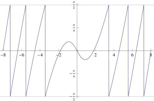
Figure 4: The phase of the complex function $\Gamma(1+ip)$

Figure 8: Many admissible spectrums of magnetic fields. If we take into account the more restrictive constrain that comes from TeV Blazars we obtain that our spectrums should remain close to scale invariance. The most blue tilted compatible spectrum is for $n_{B}\simeq 0.1$ and a scale $H_{0}=1.3\times 10^{-5}m_{pl}$. Furthermore the most red tilted magnetic fields are for $n_{B}\simeq-0.62$ and a lower scale $\sim 10^{-15}m_{pl}$

References

- (1) U. Klein, R. Wielebinski and H.W. Morsi, Astron. and Astrophys. 190 (1988) 41.
- (2) K. Kim et al., Nature 341 (1989) 720.
- (3) P.P. Kronberg, Reports on Progress in Physics 57 (1994) 325.
- (4) J. Han and R. Wielebinski, Chin. J. Astron. Astrophys. 2 (2002) 293, [arXiv:astro-ph/0209090].
- (5) C.L. Carilli and G.B. Taylor, Ann. Rev. Astron. and Astrophys. 40 (2002) 319, [arXiv:astroph/ 0110655].
- (6) J.P. Vallée, New Astron. Rev. 48 (2004) 763.
- (7) R. Beck et al., Astron. and Astrophys. 444 (2005) 739, [arXiv:astro-ph/0508485].
- (8) P.P. Kronberg et al., Astrophys. J. 676 (2008) 70, [arXiv:0712.0435].
- (9) M.L. Bernet et al., Nature 454 (2008) 302, [arXiv:0807.3347].
- (10) A. Kandus, K. E. Kunze, and C. G. Tsagas, Primordial magnetogenesis, Phys. Rept. 505 (2011) 1 58, [arXiv:1007.3891].
-
(11)
P. S. Wesson, Phys. Lett. B276: 299 (1992);
J. M. Overduin and P. S. Wesson, Phys. Rept. 283: 303 (1997). - (12) T. Liko, Space Sci. Rev. 110: 337 (2004).
- (13) J. E. Campbell, A course of Differential Geometry (Clarendon, Oxford, 1926).
- (14) L. Magaard, Zur einbettung riemannscher Raume in Einstein-Raume und konformeuclidische Raume. (PhD Thesis, Kiel, 1963).
- (15) S. Rippl, C. Romero, R. Tavakol, Class. Quant. Grav. 12: 2411 (1995).
- (16) F. Dahia, C. Romero, J. Math. Phys.43: 5804 (2002).
- (17) F. Dahia, C. Romero, Class. Quant. Grav. 22: 5005 (2005).
- (18) M.A.S.Cruz,F.Dahia,C.Romero. Mod.Phys.Lett.A23:197-203,2008[arXiv:0705.2252]
- (19) F.Dahia,C.Romero,M.A.S.Cruz. J.Math.Phys.49:112501,2008 [arXiv:0808.2025].
- (20) T.Liko, Physics Letters B 617 (2005) 193-197
- (21) J. Martin and J. Yokoyama, JCAP01(2008)025, [arXiv:0711.4307].
- (22) C. G. Tsagas, A. Kankus. Phys. Rev. D71 (2005) 123506.
- (23) J. D. Barrow, C. G. Tsagas, Phys. Rev. D77 (2008) 107302, Erratum-ibid. D77 (2008) 109904.
- (24) J. D. Barrow, C. G. Tsagas, K. Yamamoto, Phys. Rev. D86 (2012) 023533.
- (25) T. Fujita, S. Mukohyama. Universal upper limit on inflation energy scale from cosmic magnetic field. E-print: arXiv: 1205.5031.
- (26) V. Demozzi, V. Mukhanov, H. Bubinstein. JCAP 0908 (2009) 025.
- (27) S. Kanno, J. Soda, M. Watanabe. JCAP 0912 (2009) 009.
- (28) F. A. Membiela, M. Bellini. JCAP 1010: (2010) 001.
- (29) D. S. Ledesma and M. Bellini, Phys. Lett. B581: 1 (2004).
- (30) Digital Library of Mathematical Functions - National Institute of Standards and Technology. dlmf.nist.gov/10.24
- (31) J.Martin and C.Ringevla, JCAP 0608 (2006)009, [arXiv:0605367]. L.Lorenz, J.Martin y C.Ringeval [arXiv:0709.3758]
- (32) E. Kolb and M. Turner, The Early Universe, vol. 69 of Frontiers in Physics Series. Addison-Wesley Publishing Company, 1990.
- (33) A. Neronov and I. Vovk, Science 328: 73 (2010). [arXiv:1006.3504].
- (34) Tomohiro Fujita, Shinji Mukohyama. Universal upper limit on in?ation energy scale from cosmic magnetic field. E-print arXiv: 1205.5031.
- (35) A. Raya, J. E. Madriz Aguilar, M. Bellini. Phys. Lett. B638: (2006) 314.
- (36) F. A. Membiela, M. Bellini. Phys. Lett. B685: (2010) 1, Erratum-ibid. 688: (2010) 356.
- (37) J. Ponce de Leon, Gen. Rel. Grav. 20: 539 (1988).
-
(38)
B. Ratra, Astrophys. J. 391: L1 (1992);
A. D. Dolgov, Phys. Rev. 48: 2499 (1993);
F. D. Mazzitelli and F. M. Spedalieri, Phys. Rev. bf D52: 6694 (1995);
M. Gasperini, M. Giovannini and G. Veneziano, Phys. Rev. Lett. 75: 3796 (1995);
E. A. Calzetta, A. Kandus and F. D. Mazzitelli, Phys. Rev. D57: 7139 (1998);
M. S. Turner and L. M. Widrow, Phys. Rev. D37: 2743 (1998);
O. Bertolami and D. F. Mota, Phys. Lett. B455: 96 (1999);
A. -C. Davis, K. Dimopoulos, T. Prokopec and O. Törnkvist, Phys. Lett. B501: 165 (2001);
B. A. Bassett, G. Pollifrone, S. Tsujikawa and F. Viniegra, Phys. Rev. D63: 103515 (2001);
M. Gasperini, Phys. Rev. D63: 047301 (2001);
G. Lambiase and A. R. Prasanna, Phys. Rev. D70: 063502 (2004);
M. Giovannini, Phys. Rev. D76: 103508 (2007);
K. Bamba, S. Nojiri, S. D. Odintsov, Phys. Rev. D77: 123532 (2008);
K. Bamba, N. Ohta, S. Tsujikawa, Phys. Rev. D78: 043524 (2008);
K. Bamba, C. Q. Geng, S. H. Ho, JCAP 0811: 013 (2008).