A Compact Representation of the Three-Gluon Vertex

Abstract

The three-gluon vertex is a basic object of interest in nonabelian gauge theory. It contains important structural information, in particular on infrared divergences, and also figures prominently in the Schwinger-Dyson equations. At the one-loop level, it has been calculated and analyzed by a number of authors. Here we use the worldline formalism to unify the calculations of the scalar, spinor and gluon loop contributions to the one-loop vertex, leading to an extremely compact representation. The SUSY - related sum rule found by Binger and Brodsky follows from an off-shell extension of the Bern-Kosower replacement rules. We explain the relation of the structure of our representation to the low-energy effective action.

1 Introduction

The off-shell three-gluon vertex has been under investigation for more than three decades. By an analysis of the nonabelian gauge Ward identities, Ball and Chiu[1] in 1980 found a form factor decomposition of this vertex which is valid at any order in perturbation theory, with the only restriction that a covariant gauge be used. At the one-loop level, they also calculated the vertex explicitly for the case of a gluon loop in Feynman gauge. Later Cornwall and Papavassiliou[2] applied the pinch technique to the non-perturbative study of this vertex. Davydychev, Osland and Sax [3] calculated the massive quark contribution of the one loop three-gluon vertex. Binger and Brodsky[4] calculated the one-loop vertex in the pinch technique and found the following SUSY-related identity between its scalar, spinor and gluon loop contributions,

$$3\Gamma_{\rm scalar}+2\Gamma_{\rm spinor}+\Gamma_{\rm gluon}=0\\$$

In this talk, I present a recalculation of the scalar, spinor and gluon loop contributions to the three-gluon vertex using the worldline formalism [5, 6, 7, 8] . The vertex is shown in fig. 1 (for the fermion loop case).

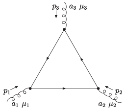
Figure 1: Three-gluon vertex.

Following the notation of [3], we write

$$\Gamma_{\mu_{1}\mu_{2}\mu_{3}}^{a_{1}a_{2}a_{3}}(p_{1},p_{2},p_{3})=-igf^{a_{1}a_{2}a_{3}}\Gamma_{\mu_{1}\mu_{2}\mu_{3}}(p_{1},p_{2},p_{3})$$ (1)

The gluon momenta are ingoing, such that $p_{1}+p_{2}+p_{3}=0$. There are actually two diagrams differing by the two inequivalent orderings of the three gluons along the loop. Those diagrams add to produce a factor of two.

The Ball-Chiu decomposition of the vertex can be written as

$$\Gamma_{\mu_{1}\mu_{2}\mu_{3}}(p_{1},p_{2},p_{3}) = A(p_{1}^{2},p_{2}^{2};p_{3}^{2})g_{\mu_{1}\mu_{2}}(p_{1}-p_{2})_{\mu_{3}}+B(p_{1}^{2},p_{2}^{2};p_{3}^{2})g_{\mu_{1}\mu_{2}}(p_{1}+p_{2})_{\mu_{3}}$$

$$+C(p_{1}^{2},p_{2}^{2};p_{3}^{2})\Big{[}p{{}_{1}}_{\mu_{2}}p{{}_{2}}_{\mu_{1}}-(p_{1}\cdot p_{2})g_{\mu_{1}\mu_{2}}\Bigl{]}(p_{1}-p_{2})_{\mu_{3}}$$

$$+\frac{1}{3}S(p_{1}^{2},p_{2}^{2},p_{3}^{2})\Bigl{[}p{{}_{1}}_{\mu_{3}}p{{}_{2}}_{\mu_{1}}p{{}_{3}}_{\mu_{2}}+p{{}_{1}}_{\mu_{2}}p{{}_{2}}_{\mu_{3}}p{{}_{3}}_{\mu_{1}}\Bigl{]}$$

$$+F(p_{1}^{2},p_{2}^{2};p_{3}^{2})\Bigl{[}(p_{1}\cdot p_{2})g_{\mu_{1}\mu_{2}}-{p_{1}}_{\mu_{2}}p{{}_{2}}_{\mu_{1}}\Bigr{]}\Bigl{[}p{{}_{1}}_{\mu_{3}}(p_{2}\cdot p_{3})-p{{}_{2}}_{\mu_{3}}(p_{1}\cdot p_{3})\Bigl{]}$$

$$+H(p_{1}^{2},p_{2}^{2},p_{3}^{2})\Big{\{}-g_{\mu_{1}\mu_{2}}\Bigl{[}p{{}_{1}}_{\mu_{3}}(p_{2}\cdot p_{3})-p{{}_{2}}_{\mu_{3}}(p_{1}\cdot p_{3})\Bigl{]}$$

$$\qquad\qquad\qquad\quad+\frac{1}{3}\Big{[}p{{}_{1}}_{\mu_{3}}p{{}_{2}}_{\mu_{1}}p{{}_{3}}_{\mu_{2}}-p{{}_{1}}_{\mu_{2}}p{{}_{2}}_{\mu_{3}}p{{}_{3}}_{\mu_{1}}\Bigl{]}\Big{\}}$$

$$+\Big{\{}{\mbox{cyclic permutations of }(p_{1},\mu_{1}),(p_{2},\mu_{2}),(p_{3},\mu_{3})}\Big{\}}$$

Here the $A$, $C$ and $F$ functions are symmetric in the first two arguments, $B$ antisymmetric, and H(S) are totally (anti)symmetric with respect to interchange of any pair of arguments. Note that the $F$ and $H$ functions are totally transverse, i.e., they vanish when contracted with any of $p_{1\mu_{1}}$, $p_{2\mu_{2}}$ or $p_{3\mu_{3}}$.

2 The scalar loop case

In the worldline formalism the three-gluon amplitude for the scalar loop case is represented as [6, 8]

$$\Gamma^{a_{1}a_{2}a_{3}}_{\rm scalar}[p_{1},\varepsilon_{1};p_{2},\varepsilon_{2};p_{3},\varepsilon_{3}]=(-ig)^{3}\mbox{tr}(T^{a_{1}}T^{a_{2}}T^{a_{3}})\int^{\infty}_{0}\frac{dT}{T}{\rm{e}}^{-m^{2}T}$$

$$\times \int\mathcal{D}x(\tau)\int_{0}^{T}d\tau_{1}\varepsilon_{1}\cdot\dot{x}_{1}\,{\rm{e}}^{ip_{1}\cdot x_{1}}\int_{0}^{\tau_{1}}d\tau_{2}\varepsilon_{2}\cdot\dot{x}_{2}\,{\rm{e}}^{ip_{2}\cdot x_{2}}\varepsilon_{3}\cdot\dot{x}_{3}\,{\rm{e}}^{ip_{3}\cdot x_{3}}~{}{\rm{e}}^{-\int_{0}^{T}\frac{\dot{x}^{2}}{4}}~{}~{}~{}$$

Here $T$ is the total proper time of the loop particle, $m$ the mass of the loop particle, $T^{a}$ a generator of the gauge group in the representation of the scalar, and $\int\mathcal{D}(x)$ an integral over closed trajectories in Minkowski space-time with periodicity $T$. Although our calculation will be off-shell, we introduce gluon polarization vectors $\varepsilon_{i}$ as a book-keeping device. Each gluon is represented by a vertex operator $\int d\tau\varepsilon\cdot\dot{x}\,{\rm{e}}^{ip\cdot x}\rm$. Translation inveriance in proper-time has been used to set $\tau_{3}=0$.

The path integral (LABEL:bk) is Gaussian so that its evaluation requires only the standard combinatorics of Wick contractions and the appropriate Green’s function,

$$<x^{\mu_{1}}(\tau_{1})x^{\mu_{2}}(\tau_{2})>=\!-G_{B12}g^{\mu_{1}\mu_{2}},\,G_{B12}:=G_{B}(\tau_{1},\tau_{2})=|\tau_{1}-\tau_{2}|-\frac{(\tau_{1}-\tau_{2})^{2}}{T}~{}~{}~{}~{}~{}~{}~{}~{}~{}~{}~{}~{}~{}$$

(4)

In this formalism structural simplification can be expected from the removal of all second derivatives $\ddot{G}_{Bij}$’s , appearing after the Wick contractions, by suitable integrations by part (IBP). After doing this we have (see[8] for the combinatorial details of the Wick contraction and IBP procedure)

$$\Gamma_{\rm scalar} = \frac{g^{3}}{(4\pi)^{D/2}}(\Gamma_{\rm scalar}^{3}+\Gamma_{\rm scalar}^{2}+\Gamma_{\rm scalar}^{\rm bt})$$

$$\Gamma_{\rm scalar}^{3} = -{\mbox{t}r}(T^{a_{1}}[T^{a_{2}},T^{a_{3}}])\int_{0}^{\infty}\frac{dT}{T^{\frac{D}{2}}}{\rm e}^{-m^{2}T}\int_{0}^{T}d\tau_{1}\int_{0}^{\tau_{1}}d\tau_{2}\,Q_{3}^{3}|_{\tau_{3}=0}~{}{\rm e}^{(G_{B12}p_{1}\cdot p_{2}+G_{B13}p_{1}\cdot p_{3}+G_{B23}p_{2}\cdot p_{3})}$$

$$\Gamma_{\rm scalar}^{2} = \Gamma_{\rm scalar}^{3}(Q_{3}^{3}\to Q_{3}^{2})$$

$$\Gamma_{\rm scalar}^{\rm bt} = -{\mbox{t}r}(T^{a_{1}}[T^{a_{2}},T^{a_{3}}])\int_{0}^{\infty}\frac{dT}{T^{\frac{D}{2}}}{\rm e}^{-m^{2}T}\int_{0}^{T}d\tau_{1}\dot{G}_{B12}\dot{G}_{B21}\Bigl{[}\varepsilon_{3}\cdot f_{1}\cdot\varepsilon_{2}~{}{\rm e}^{G_{B12}p_{1}\cdot(p_{2}+p_{3})}+{\rm 2\,perm}\Bigr{]}$$

$$Q_{3}^{3} = \dot{G}_{B12}\dot{G}_{B23}\dot{G}_{B31}{\mbox{t}r}(f_{1}f_{2}f_{3})$$

$$Q_{3}^{2} = \frac{1}{2}\dot{G}_{B12}\dot{G}_{B21}{\mbox{t}r}(f_{1}f_{2})\sum_{k=1,2}\dot{G}_{B3k}\varepsilon_{3}\cdot p_{k}+{\rm 2\,perm}$$

The abelian field strength tensors $f^{\mu\nu}_{i}:=p_{i}^{\mu}\varepsilon_{i}^{\nu}-\varepsilon_{i}^{\mu}p_{i}^{\nu}$ appear automatically in the IBP procedure. The $\Gamma_{\rm scalar}^{\rm bt}$’s are boundary terms of the IBP.

We rescale to the unit circle, $\tau_{i}=Tu_{i},i=1,2,3,$ and rewrite these integrals in term of the standard Feynman/Schwinger parameters, related to the $u_{i}$ by

$$u_{1}=\alpha_{2}+\alpha_{3}~{}~{}~{},~{}~{}~{}u_{2}=\alpha_{3}~{}~{}~{},~{}~{}~{}u_{3}=0~{}~{}~{},~{}~{}~{}\alpha_{1}+\alpha_{2}+\alpha_{3}=1$$ (6)

For the scalar case, we find

$$\Gamma_{\rm scalar} = \frac{g^{3}}{(4\pi)^{\frac{D}{2}}}\mbox{tr}(T^{a_{1}}[T^{a_{2}},T^{a_{3}}])(\gamma_{\rm scalar}^{3}+\gamma_{\rm scalar}^{2}+\gamma_{\rm scalar}^{\rm bt})$$

$$\gamma_{\rm scalar}^{3} = \Gamma\bigl{(}3-\frac{D}{2}\bigr{)}\mbox{tr}(f_{1}f_{2}f_{3})I^{D}_{3,B}(p_{1}^{2},p_{2}^{2},p_{3}^{2})$$

$$\gamma_{\rm scalar}^{2} = \frac{1}{2}\Gamma\bigl{(}3-\frac{D}{2}\bigr{)}\Bigl{[}\mbox{tr}(f_{1}f_{2})\Bigl{(}\varepsilon_{3}\cdot p_{1}I^{D}_{2,B}(p_{1}^{2},p_{2}^{2},p_{3}^{2})-\varepsilon_{3}\cdot p_{2}I^{D}_{2,B}(p_{2}^{2},p_{1}^{2},p_{3}^{2})\Bigr{)}+{\rm 2\,perm}\Bigr{]}$$

$$\gamma_{\rm scalar}^{\rm bt} = -\Gamma\bigl{(}2-\frac{D}{2}\bigr{)}\Bigl{[}\varepsilon_{3}\cdot f_{1}\cdot\varepsilon_{2}I^{D}_{{\rm bt},B}(p_{1}^{2})+{\rm 2\,perm}\Bigr{]}$$

where

$$I_{3,B}^{D}(p_{1}^{2},p_{2}^{2},p_{3}^{2}) = \int_{0}^{1}d{\alpha}_{1}d{\alpha}_{2}d{\alpha}_{3}\delta(1-{\alpha}_{1}-{\alpha}_{2}-{\alpha}_{3})$$

$$\times \frac{(1-2{\alpha}_{1})(1-2{\alpha}_{2})(1-2{\alpha}_{3})}{\Bigl{(}m^{2}+{\alpha}_{1}{\alpha}_{2}p_{1}^{2}+{\alpha}_{2}{\alpha}_{3}p_{2}^{2}+{\alpha}_{1}{\alpha}_{3}p_{3}^{2}\Bigr{)}^{3-\frac{D}{2}}}$$

$$I_{2,B}^{D}(p_{1}^{2},p_{2}^{2},p_{3}^{2}) = \int_{0}^{1}d{\alpha}_{1}d{\alpha}_{2}d{\alpha}_{3}\delta(1-{\alpha}_{1}-{\alpha}_{2}-{\alpha}_{3})$$

$$\times \frac{(1-2{\alpha}_{2})^{2}(1-2{\alpha}_{1})}{\Bigl{(}m^{2}+{\alpha}_{1}{\alpha}_{2}p_{1}^{2}+{\alpha}_{2}{\alpha}_{3}p_{2}^{2}+{\alpha}_{1}{\alpha}_{3}p_{3}^{2}\Bigr{)}^{3-\frac{D}{2}}}$$

$$I_{bt,B}^{D}(p^{2}) = \int_{0}^{1}d{\alpha}\frac{(1-2{\alpha})^{2}}{\bigl{(}m^{2}+{\alpha}(1-{\alpha})p^{2}\bigr{)}^{2-\frac{D}{2}}}$$

3 Fermion and gluon loop calculations

By an off-shell generalization of the Bern-Koswer replacement rules [5], whose correctness for the case at hand we have verified, one can get the results for the spinor and gluon loop from the scalar loop one simply by replacing

$$\Gamma_{\rm scalar}\rightarrow\Gamma_{\rm spinor}:~{}~{}~{}~{}I_{\{3,2,{\rm bt}\},B}^{D}\rightarrow I_{\{3,2,{\rm bt}\},B}^{D}-I_{\{3,2,{\rm bt}\},F}^{D}$$

$$\Gamma_{\rm scalar}\rightarrow\Gamma_{\rm gluon}:~{}~{}~{}~{}~{}~{}I^{D}_{\{3,2,{\rm bt}\},B}\rightarrow I^{D}_{\{3,2,{\rm bt}\},B}-4I^{D}_{\{3,2,{\rm bt}\},F}$$

(9)

where the $I^{D}_{(\cdot)F}$’s are three integrals similar to the $I^{D}_{(\cdot)B}$’s above (for the spinor loop one must also multiply by a global factor of $-2$).

From (9) we immediately recover the Binger-Brodsky identity eq.(1).

4 Comparison with the effective action

Finally let us compare our results with the low energy expansion of the QCD effective action induced by a scalar loop,

$$\Gamma_{{\rm scalar}}[F]=\int_{0}^{\infty}\frac{dT}{T}\frac{{{\rm e}}^{-m^{2}T}}{(4\pi T)^{\frac{D}{2}}}{{\rm tr}}\int dx_{0}\sum_{n=2}^{\infty}\frac{(-T)^{n}}{n!}{{\rm O}}_{n}[F]$$ (10)

For our comparison we need only $O_{2}$ and $O_{3}$ which are[8]

$$O_{2}=-\frac{1}{6}F_{\kappa\lambda}F^{\kappa\lambda}~{}~{}~{},~{}~{}~{}O_{3}=-\frac{2}{15}iF_{\kappa}^{~{}\lambda}F_{\lambda}^{~{}\mu}F_{\mu}^{~{}\kappa}-\frac{1}{20}D_{\kappa}F_{\lambda\mu}D^{\kappa}F^{\lambda\mu}~{}~{}$$ (11)

where

$$F_{\mu\nu}=f_{\mu\nu}+ig[A_{\mu},A_{\nu}]~{}~{},~{}~{}~{}f_{\mu\nu}=\partial_{\mu}A_{\nu}-\partial_{\nu}A_{\mu}~{}~{},~{}~{}D_{\mu}=\partial_{\mu}+igA_{\mu}$$ (12)

We can recognize the correspondences

$$\gamma_{(\cdot)}^{3}\leftrightarrow F_{\kappa}^{~{}\lambda}F_{\lambda}^{~{}\mu}F_{\mu}^{~{}\kappa}=f_{\kappa}^{\lambda}f_{\lambda}^{\mu}f_{\mu}^{\kappa}+{\rm higher~{}point~{}terms}$$

$$\gamma_{(\cdot)}^{2}\leftrightarrow(\partial+ig\underbrace{A)F(\partial}+igA)F$$

$$\gamma_{(\cdot)}^{\rm bt}\leftrightarrow(f+ig\underbrace{[A,A])(f}+ig[A,A])$$

(13)

5 Conclusions and outlook

In our recalculation of the scalar, spinor and gluon contributions to the one-loop three gluon vertex we have achieved a significant improvement over previous calculations both in efficiency and compactness of the result. This improvement is in large part due to the replacement rules (9) whose validity off-shell we have verified. Details and a comparison with the Ball-Chiu decomposition will be presented elsewhere. We believe that along the lines presented here even a first calculation of the four-gluon vertex would be feasible.

References

• [1] J. S. Ball and T. W. Chiu, Phys. Rev. D 22, 2550 (1980).
• [2] J. M Cornwall and J. Papavassiliou, Phys. Rev. D 40, 3474 (1989).
• [3] A. I. Davydychev, P. Osland and L. Saks, JHEP 0108:050 (2001).
• [4] M. Binger and S. J. Brodsky, Phys. Rev. D 74, 054016 (2006).
• [5] Z. Bern and D. A. Kosower, Phys. Rev. Lett. 66, 1669 (1991); Nucl. Phys. B 379, 451 (1992).
• [6] M. J. Strassler, Nucl. Phys. B 385, 145 (1992).
• [7] M. Reuter, M. G. Schmidt and C. Schubert, Ann. Phys. (N.Y.) 259, 313 (1997).
• [8] C. Schubert, Phys. Rept. 355, 73 (2001).