Efficiency at maximum power output of an irreversible Carnot-like cycle with internally dissipative friction

Abstract

We investigate the efficiency at maximum power of an irreversible Carnot engine performing finite-time cycles between two reservoirs at temperatures $T_{h}$ and $T_{c}$ $(T_{c}<T_{h})$, taking into account of internally dissipative friction in two “adiabatic” processes. In the frictionless case, the efficiencies at maximum power output are retrieved to be situated between $\eta_{{}_{C}}/$ and $\eta_{{}_{C}}/(2-\eta_{{}_{C}})$, with $\eta_{{}_{C}}=1-T_{c}/{T_{h}}$ being the Carnot efficiency. The strong limits of the dissipations in the hot and cold isothermal processes lead to the result that the efficiency at maximum power output approaches the values of $\eta_{{}_{C}}/$ and $\eta_{{}_{C}}/(2-\eta_{{}_{C}})$, respectively. When dissipations of two isothermal and two adiabatic processes are symmetric, respectively, the efficiency at maximum power output is founded to be bounded between $0$ and the Curzon-Ahlborn (CA) efficiency $1-\sqrt{1-\eta{{}_{C}}}$, and the the CA efficiency is achieved in the absence of internally dissipative friction.

Keywords: heat engine, finite-time cycle, friction.

PACS number(s): 05.70.Ln, 05.30.-d

I introduction

Quasistatic Carnot cycle is the most efficient heat engine cycle allowed by physical laws. Practically any heat engine operates far from the ideal maximum efficiency conditions set by Carnot Car24 . Although the Carnot cycle has the highest efficiency, its power output is zero because the time for completing a cycle is infinite. The cycle should be speeded up to obtain a finite power. Considering a finite-time Carnot cycle within the assumption of endoreversibility that irreversible processes occur only through the heat exchanges, Curzon and Ahlborn (CA) Cur75 obtained the efficiency at maximum power output as

$$\eta_{{}_{CA}}=1-\sqrt{{T_{c}}/{T_{h}}},$$ (1)

where $T_{h}$ and $T_{c}$ are the temperatures of the hot and cold heat reservoirs, respectively. Historically speaking, the seminal expression (1) was derived by Yvon Yvo55 and Novikov Nov58 much earlier than Cur75 . But it is usually called the CA efficiency. Recently, the issue of the efficiency at maximum power output, as main focus of finite time thermodynamics, has attracted much interest Che89 ; Esp10 ; Esp09 ; Esp11 ; Ape12 ; Oue12 ; pre11 ; pre12I ; pre12II ; Gor91 ; Sch08 ; Tu08 ; Tu12 ; Gav10 ; Mor12 ; Van05 ; Izu08 ; Gev92 ; Fel00 ; Rez06 ; Abe11 ; Wang11 ; Chen11 ; Sei11 ; Tu48 . Under the low-dissipation assumption that the irreversible entropy production in a heat-exchange process is inversely proportional to the time required for completing that process, Esposito et al. Esp10 proposed a model for low-dissipation Carnot-like engines, in which use of endoreversibility hypothesis and phenomenological transfer laws can be avoided .

Although the importance of internally frictional dissipation in an adiabatic process was mentioned by Novikov in his pioneer paper Nov58 ; note1 , most of the studies about the efficiency at maximum power output always neglect the influence of inner friction on the performance of the heat engine models, within the assumption that the time taken for completing the adiabatic process is ignored or proportional to the total time spent on the isothermal processes. From everyday experience, the irreversible phenomena that limits the optimal performance of engines occurs not only in an isothermal process but but also in an adiabatic process because of inner friction when classical or quantum piston moves Jar12 ; Nak11 ; Fel00 ; Gor91 ; Rez06 ; Biz12 . Dissipation loss due to internally dissipative friction, by which real engines are dominated Gor91 , has been discussed in several papers Fel00 ; Wang07 ; Rez06 ; Wu92 ; pre12I . However, so far there has been no comprehensive discussion of the effects of friction on the cycle performance in the literature, and thus the properties of an irreversible Carnot-like cycle consisting of two irreversible isothermal and two non-isentropic adiabatic processes have not been addressed adequately and clearly. For this reason, we follow the tradition of thermodynamics constructing a more generalized engine, in which the “adiabatic” process takes finite time as well as becoming non-isentropic Wang07 ; Fel00 ; Rez06 ; Nak11 ; adia . Troughout this paper, the word “isothermal” merely indicates that the working substance is in contact with a reservoir at constant temperature, and the word “adiabatic” means that the working substance is isolated from a heat reservoir and no heat exchange happens.

In this paper, we focus on the study of the efficiency at maximum power output of an irreversible Carnot-like engine performing finite time cycles, in which frictional dissipation and the time of any adiabat are taken into account. We derive the cycle period which contains time spent on four thermodynamic processes, which is quite different from that derived in the previous models for which the time of two adiabatic processes was assumed to either be proportional to the time duration of the two isothermal processes or be negligible. In the frictionless case, the efficiencies at maximum power output are proved to bounded between $\eta_{{}_{C}}/$ and $\eta_{{}_{C}}/(2-\eta_{{}_{C}})$, with the Carnot efficiency $\eta_{{}_{C}}=1-T_{c}/{T_{h}}$, coinciding with the result found in Ref. Esp10 for frictionless engine models in which the time required for completing any adiabatic process was assumed to be totally ignored. In the strong limits of the dissipations in the hot and cold isothermal processes, we find that the efficiency at maximum power output approaches the values of $\eta_{{}_{C}}/$ and $\eta_{{}_{C}}/(2-\eta_{{}_{C}})$, respectively. If dissipations of two isothermal and two adiabatic processes are symmetric, respectively, we prove that the efficiency at maximum power output is bounded between $0$ and the Curzon-Ahlborn (CA) efficiency $1-\sqrt{1-\eta{{}_{C}}}$, and that the CA efficiency is reached by ignoring the friction.

II Engine model

A Carnot-like cycle $1\rightarrow 2\rightarrow 3\rightarrow 4\rightarrow 1$ is drawn in the $(S,T)$ plane (see Fig. 1 ). During two isothermal processes $1\rightarrow 2$ and $3\rightarrow 4$, the working substance is coupled to a hot and a cold heat reservoir at constant temperatures $T_{h}$ and $T_{c}$, respectively. Let $S_{i}$ be the entropies at the instants $i$ with $i=1,2,3,4$. For the reversible cycle where $S_{2}=S_{3}$ and $S_{1}=S_{4}$, we recover the Carnot efficiency $\eta_{{}_{C}}=1-\frac{T_{c}}{T_{h}}$, which is independent of the properties of the working substance. In the adiabatic process $2\rightarrow 3$ ($4\rightarrow 1$), the working substance is decoupled from the hot (cold) reservoir, and the entropy changes from $S_{2}$ to $S_{3}$ ($S_{4}$ to $S_{1}$) in a period $t_{a}$ ( $t_{b}$).

Let us consider the Carnot-like cycle under finite-time operation. Finite-time cycles move the working substance away from the equilibrium, leading to irreversibility of the engine. Although the system needs no close to equilibrium during the isothermal process, the system remains in an equilibrium state with the heat reservoir at the special instants $i$ where $i=1,2,3,4$. Under such a circumstance, the thermodynamic quantities of the system$-$in particular the entropy$-$are well defined at these instants. Unlike in the frictionless case where any adiabatic process is isentropic, the adiabatic process becomes non-isentropic when friction is included, since friction develops heat and leads to an increase in entropy in any adiabat. This additional heat remains in chamber or in trap along an adiabatic process until it is released to a heat reservoir with which the working systems couples during an isothermal process. As a consequence, heat productions due to friction in the adiabatic expansion $2\rightarrow 3$ and in the adiabatic compression $4\rightarrow 1$ are released into the cold and hot reservoirs, respectively Ape12 ; Wu92 . This additional heat is also represented in Fig. 1 by the red triangular area for the branch $2\rightarrow 3$ and by the blue triangular area for the process $4\rightarrow 1$. Note that, the heat produced during the process $4\rightarrow 1$ decreases the absorbed heat during the hot isothermal process, and the heat produced during the adiabat $2\rightarrow 3$, as pure loss, is released to the cold reservoir. The cycle model is operated in the following processes.

Figure 1: (Color online) Schematic diagram of an irreversible Carnot-like cycle in the plane of the temperature $T$ and entropy $S$. The values of the entropy $S$ at the four special instants are indicated. $t_{h}$ ($t_{c}$) is the time allocation when in contact with the hot (cold) reservoir. $t_{a}$ represents the time allocation for adiabatic expansion and $t_{b}$ for adiabatic compression. The red triangular area is the heat developed by friction for the process $2\rightarrow 3$, while the blue triangular area represents the additional heat for the process $4\rightarrow 1$.

1. Isothermal expansion $1\rightarrow 2$ . At time $t=0$, the working substance is brought into contact with a hot reservoir at constant temperature $T_{h}$. The hot reservoir is then removed after time duration $t_{h}$. An amount of heat absorbed from the surroundings is represented by $Q_{h}$. In this process, the entropy is changing from the initial entropy $S_{1}$ to the entropy $S_{2}$. The entropy variation, $\Delta S_{h}=S_{2}-S_{1}$, is given by

$$\Delta S_{h}=Q_{h}/{T_{h}}+\Delta S^{ir}_{h},$$ (2)

where $\Delta S^{ir}_{h}$ is the irreversible entropy production.

2. Adiabatic expansion $2\rightarrow 3$. The working substance decouples from the hot reservoir for a time duration $t_{a}$. In this process the frictional dissipation develops heat, resulting in the fact that the entropy increases from $S_{2}$ to $S_{3}$. The entropy production arising from the inner friction is denoted by

$$\Delta S_{a}=S_{3}-S_{2}=\Delta S^{ir}_{a}.$$ (3)

3. Isothermal compression $3\rightarrow 4$. The working substance is coupled to a cold reservoir at constant temperature $T_{c}$ for time $t_{c}$. Then entropy changes on this process from $S_{3}$ to the entropy $S_{4}$. For the cycle to close, $S_{4}$ should be smaller than $S_{1}$. The variation of the entropy can be expressed as

$$\Delta S_{c}=|S_{3}-S_{4}|=Q_{c}/{T_{c}}+\Delta S^{ir}_{c},$$ (4)

where $Q_{c}$ is the amount of heat released directly to the cold reservoir, and $\Delta S^{ir}_{c}$ is the irreversible entropy production.

4. Adiabatic compression $4\rightarrow 1$. Similar to the adiabatic expansion, the working substance decouples from cold reservoir. The time required for completing this process reads $t_{b}$. The entropy increases from $S_{4}$ to the original value $S_{1}$. The amount of entropy production due to the internally frictional dissipation during this process is given by

$$\Delta S_{b}=S_{1}-S_{4}=\Delta S_{b}^{ir}.$$ (5)

After performing a whole cycle, the system recovers the initial state and thus its total energy remains unchanged for the whole cycle. The work output after a single cycle can be expressed as

$$W=Q_{h}-Q_{c}={(T_{h}-T_{c})}\Delta S-T_{h}(\Delta S^{ir}_{h}+\frac{S^{ir}_{b}}{2})-T_{c}(\Delta S^{ir}_{c}+\frac{S^{ir}_{a}}{2}),$$ (6)

where $\Delta S\equiv S_{2}-S_{1}$ is a state variable only depending on the initial and final states of the isothermal processes, whereas, $\Delta S^{ir}_{h}$, $\Delta S^{ir}_{c}$, $\Delta S^{ir}_{a}$, and $\Delta S^{ir}_{b}$ are process variables depending on the detailed protocols.

III Efficiency at maximum power output

To continue our analysis, we denote, by min$\left\{\Delta S^{ir}_{\kappa}\right\}\equiv L_{\kappa}(t_{\kappa})$ Sch08 ; Esp10 ; Gor91 ; Fel00 ; Tu12 ; Bli12 ; Wang07 ; Tuar with $\kappa=h,c,a,$ and $b$, the minimum irreversible entropy production for the optimized protocols. Physically, the larger time required for completing the corresponding process, the closer the process is to quasistatic process, indicating that the irreversible entropy productions $S_{\kappa}$ become much smaller and tend to be zero in the longtime limits ($t_{\kappa}\rightarrow\infty)$. In other words, $L_{\kappa}(t_{\kappa})$ should be a monotonous decreasing function of $t_{\kappa}$ for a given process $\kappa$. Because the irreversible entropy production $L_{\kappa}$ is a function of the time $t_{\kappa}$ for a given process $\kappa$, the irreversible entropy production $L_{a}(t_{a})$ [$L_{b}(t_{b})$] in the adiabatic process $2\rightarrow 3$ ($4\rightarrow 1$) can not be included by the irreversible entropy production $L_{c}(t_{c})$ [$L_{h}(t_{h})$] during the cold (hot) isothermal process.

For convenience, we make a variable transformation $x_{\kappa}=1/{t_{\kappa}}$ with $\kappa=h,c,a$ and $b$, and have the cycle time $\tau=t_{h}+t_{c}+t_{a}+t_{b}=1/x_{h}+1/x_{c}+1/x_{a}+1/x_{b}$. Accordingly, the power output $P=W/\tau$ and the efficiency $\eta=W/Q_{h}$ are

$$P=\frac{(T_{h}-T_{c})\Delta S-T_{h}[L_{h}(x_{h})+L_{b}(x_{b})/2]-T_{c}\left[L_{c}(x_{c})+L_{a}(x_{a})/2\right]}{(1/x_{h}+1/x_{c}+1/x_{a}+1/x_{b})},$$ (7)

and

$$\eta=\frac{{(T_{h}-T_{c})}\Delta S-T_{h}\left[L_{h}(x_{h})+L_{b}(x_{b})/2\right]-T_{c}\left[L_{c}(x_{c})+L_{a}(x_{a})/2\right]}{T_{h}\left[\Delta S-L_{h}(x_{h})-L_{b}(x_{b})/2\right]},$$ (8)

respectively.

To specify the time allocation at maximum power output, the values of $x_{\kappa}$, with $\kappa=h,c,a$ and $b$, should be optimized. We optimize power output $P$ over the time variables $x_{\kappa}$ to obtain the time allocation during a cycle and thus to determine the corresponding efficiency. Setting the derivatives of $P$ with respect to $x_{\kappa}$ ($\kappa=h,c,a,b$) equal to zero, we derive the following equations:

$$T_{h}L^{\prime}_{h}x_{h}^{2}=W,$$ (9)

$$T_{c}L^{\prime}_{c}x_{c}^{2}=W,$$ (10)

$$T_{c}L^{\prime}_{a}x_{a}^{2}=2W,$$ (11)

$$T_{h}L^{\prime}_{b}x_{b}^{2}=2W,$$ (12)

where the work $W$ was defined in Eq. (6), and $L^{\prime}_{\kappa}=\frac{dL_{\kappa}}{dx_{\kappa}}$ with $\kappa=h,c,a,b$. Dividing Eq. (9) by Eqs. (10), (11), and (12), respectively, we find the optimal time allocation at maximum power output:

$$\frac{x_{c}}{x_{h}}=\sqrt{\frac{T_{h}L^{\prime}_{h}}{T_{c}L^{\prime}_{c}}},$$ (13)

$$\frac{x_{a}}{x_{h}}=\sqrt{\frac{2T_{h}L^{\prime}_{h}}{T_{c}L^{\prime}_{a}}},$$ (14)

$$\frac{x_{b}}{x_{h}}=\sqrt{\frac{2L^{\prime}_{h}}{L^{\prime}_{b}}}.$$ (15)

Now we turn to the low-dissipation case where one assumes $L^{\prime}_{\kappa}(x_{\kappa})=\Sigma_{\kappa}$ with $\Sigma_{\kappa}$ being dissipation constants. In this case, we find, by substituting Eqs. (13), (14), and (15) into the maximization condition $\frac{\partial P}{\partial x_{h}}=0$, the physical solution at

$$x_{h}=\frac{\Delta S(T_{h}-T_{c})}{2T_{h}\Sigma_{h}\left(1+\sqrt{\frac{T_{c}\Sigma_{c}}{T_{h}\Sigma_{h}}}\right)},$$ (16)

$$x_{c}=\frac{\Delta S(T_{h}-T_{c})}{2T_{c}\Sigma_{c}\left(1+\sqrt{\frac{T_{h}\Sigma_{h}}{T_{c}\Sigma_{c}}}\right)},$$ (17)

$$x_{a}=\frac{\Delta S(T_{h}-T_{c})}{T_{c}\Sigma_{a}\left(\sqrt{\frac{2\Sigma_{c}}{\Sigma_{a}}}+\sqrt{\frac{2T_{h}\Sigma_{h}}{T_{c}\Sigma_{a}}}\right)},$$ (18)

$$x_{b}=\frac{\Delta S(T_{h}-T_{c})}{T_{h}\Sigma_{b}\left(\sqrt{\frac{2\Sigma_{h}}{\Sigma_{b}}}+\sqrt{\frac{2T_{c}\Sigma_{c}}{T_{h}\Sigma_{b}}}\right)}.$$ (19)

The expressions (16) and (17) of the times spent on a hot and cold isothermal process for a frictional heat engine are, respectively, identical to corresponding ones [Eq. (7)] obtained a engine model Esp10 in which both the internally dissipative friction and the time taken for two adiabats were assumed to be zero.

Using Eq. (8), together with Eqs. (16), (17), (18), and (19), it follows that the efficiency at maximum power becomes

$$\eta^{*}=\frac{\eta_{{}_{C}}\left(1+\sqrt{\frac{T_{c}\Sigma_{c}}{T_{h}\Sigma_{h}}}-\sqrt{\frac{T_{c}\Sigma_{a}}{2T_{h}\Sigma_{h}}}-\sqrt{\frac{\Sigma_{b}}{2\Sigma_{h}}}\right)}{1+2\sqrt{\frac{T_{c}\Sigma_{c}}{T_{h}\Sigma_{h}}}+\frac{T_{c}}{T_{h}}-\sqrt{\frac{\Sigma_{b}}{2\Sigma_{h}}}\left(1-\frac{T_{c}}{T_{h}}\right)},$$ (20)

which is one of our main results in the paper. Unlike the frictionless cycle where the positive work condition is $T_{c}<T_{h}$, the frictional cycle produces positive work under the conditions that $T_{c}<T_{h}$ and

$$\sqrt{\Sigma_{a}}+\sqrt{\frac{T_{c}}{T_{h}}}\sqrt{\Sigma_{b}}<\sqrt{2}(\sqrt{\Sigma_{h}}+\sqrt{\frac{T_{c}}{T_{h}}}\sqrt{\Sigma_{c}}).$$ (21)

Only when this positive work condition is satisfied can the positive work be extracted. We present the efficiency at maximum power output in a broader context by taking into account of inner friction and the time taken for any adiabat.

(1) When the inner friction is neglected, i.e., $\Sigma_{a}\rightarrow 0$ and $\Sigma_{b}\rightarrow 0$, the expression (20) of efficiency at maximum power output is reduced to that from either stochastic thermodynamics Sch08 or by low-dissipation assumption Esp10 . In this frictionless case, the completely asymmetric limits $\frac{\Sigma_{c}}{\Sigma_{h}}\rightarrow 0$ and $\frac{\Sigma_{c}}{\Sigma_{h}}\rightarrow\infty$, causing the efficiency $\eta_{m}$ at maximum power to approach the upper and lower bounds at $\eta_{+}\equiv\frac{\eta_{{}_{C}}}{2-\eta_{{}_{C}}}$ and $\eta_{-}\equiv\frac{\eta_{{}_{C}}}{2}$, respectively. That is, when $\Sigma_{a}\rightarrow 0$ and $\Sigma_{b}\rightarrow 0$, the result of the the bounds of the efficiency at maximum power for frictionless Carnot-like cycle is retrieved,

$$\frac{\eta_{{}_{C}}}{2}\equiv\eta_{-}\leq\eta_{m}\leq\eta_{+}\equiv\frac{\eta_{{}_{C}}}{2-\eta_{{}_{C}}}.$$ (22)

For the symmetric dissipation ${\Sigma_{c}}={\Sigma_{h}},$ the time allocation to the hot and cold processes satisfies

$$\frac{t_{h}}{t_{c}}=\sqrt{\frac{T_{h}}{T_{c}}},$$ (23)

from which we can arrive at the CA efficiency $\eta^{*}=\eta_{{}_{CA}}=1-\sqrt{\frac{T_{c}}{T_{h}}}$ by using Eq. (20). We would like to emphasize that the results are identical to those in Ref. Esp10 , but they are derived in the generalized engine model in which the times required for completing two adiabatic processes in the Carnot-like cycle are obtained as Eqs. (14) and (15).

(2) The values of frictional dissipations both $\Sigma_{a}$ and $\Sigma_{b}$ are nonzero but finite. In the limits ${\Sigma_{h}}\rightarrow\infty$ and ${\Sigma_{c}}\rightarrow\infty$, the efficiency at maximum power output $\eta^{*}$ in Eq. (20) converges to the upper bound $\eta_{+}=\frac{\eta_{{}_{C}}}{2-\eta_{{}_{C}}}$ and to the lower bound $\eta_{-}=\frac{\eta_{{}_{C}}}{2}$, respectively. Here the lower and upper bounds are identical to the corresponding ones in previous studies, but extended to the irreversible Carnot-like cycle in which any adiabatic process is irreversible because of internally frictional dissipation and its time is not negligible.

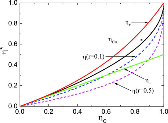
Figure 2: (Color online) Efficiency $\eta^{*}$ at maximum power as a function of the Carnot value $\eta_{{}_{C}}$. The upper and lower bounds of efficiency at maximum power output in the frictionless case $\eta_{+}$ and $\eta_{-}$, the CA efficiency $\eta_{{}_{CA}}$, and the efficiencies for $r=0.1$ and $r=0.5$, are indicated in the figure.

(3) Dissipations in two isothermal and two adiabatic processes are symmetric, respectively, $\Sigma_{h}=\Sigma_{c}=r\Sigma_{a}=r\Sigma_{b}=r\Sigma$ with $r$ and $\Sigma$ being constants. Then the efficiency at maximum power becomes

$$\eta^{*}=\frac{\eta_{{}_{C}}{(\sqrt{r/2}-1)\left(1+\sqrt{1-\eta_{{}_{C}}}\right)}}{-2\left(1+\sqrt{1-\eta_{{}_{C}}}\right)+\eta_{{}_{C}}(\sqrt{r/2}+1)},$$ (24)

which satisfies the relation

$$0<\eta^{*}\leq\eta_{{}_{CA}}=1-\sqrt{1-\eta_{{}_{C}}}.$$ (25)

Compared with the bounds (22) for frictionless case, both the upper and lower bounds (25) of the efficiency at maximum power are lowered when friction is introduced. Physically, this originates from the fact that dissipative work is done to overcome the inner friction which generates heat. When $r\rightarrow\sqrt{2}$, no positive work is extracted from the cycle,thereby indicating that the efficiency becomes equal to zero. From Eqs. (13), (14), and (15), we find that the times spent on the four quantum thermodynamic processes are distributed in such a way that

$${t_{h}}/{t_{c}}={t_{b}}/{t_{a}}=\sqrt{{T_{h}}/{T_{c}}},$$ (26)

with ${t_{h}}/{t_{b}}=\sqrt{r}$. It should be noted that the efficiency at maximum power increases as $r$ decreases, approaching the CA efficiency $\eta_{{}_{CA}}$ in the frictionless limit ($r\rightarrow 0$). In Fig. 2 we plot the efficiency (24) as a function of $\eta_{{}_{C}}$ for $r=0.1$ and $r=0.5$, comparing $\eta_{{}_{CA}}$ with the upper and lower bounds $\eta_{+}$ and $\eta_{-}$ of frictionless engine models.

IV Conclusions

In conclusion, we have determined the efficiency at maximum power for an irreversible Carnot-like engine which performs finite-time cycles with internally dissipative friction. In the limits of extremely asymmetric dissipation ($\frac{\Sigma_{c}}{\Sigma_{h}}\rightarrow 0$ and $\frac{\Sigma_{c}}{\Sigma_{h}}\rightarrow\infty$, with $\frac{\Sigma_{a}}{\Sigma_{h}}\rightarrow 0$ and $\frac{\Sigma_{b}}{\Sigma_{h}}\rightarrow 0$), the efficiency at maximum power output converges to an upper and a lower bound $\frac{\eta_{{}_{C}}}{2-\eta_{{}_{C}}}$ and $\frac{\eta_{{}_{C}}}{2}$, coinciding with the result obtained previously in the frictionless engine model in which the time taken for two adiabatic processes was ignored. When the dissipation in the hot (cold) isothermal process approaches the strong limit, i.e., $\Sigma_{h}\rightarrow\infty$ ($\Sigma_{c}\rightarrow\infty$), the efficiency at maximum power output tends to be the upper (lower) bound $(\frac{\eta_{{}_{C}}}{2-\eta_{{}_{C}}})$ ($\frac{\eta_{{}_{C}}}{2}$). When the dissipations in two isothermal and two adiabatic processes are symmetric, respectively, we find that the efficiency at maximum power output is bounded from above by the CA efficiency $\eta_{{}_{CA}}$ and from below by zero, and that $\eta_{{}_{CA}}$ is reached in the frictionless limit.

Acknowledgements: We gratefully acknowledge support for this work by the National Natural Science Foundation of China under Grants No. 11147200 and No. 11065008, and the Foundation of Jiangxi Educational Committee under Grant No. GJJ12136. J. H. Wang is also grateful for helpful discussions with Yann Apertet and Zhanchun Tu.

References

- (1) S. Carnot, Réflexions sur la PuissanceMotrice du Feu set sur les Machines Propres à D́evelopper cette Puissance (self-published, Paris, 1824).
- (2) F. Curzon and B. Ahlborn, Am. J. Phys. 43, 22 (1975).
- (3) J. Yvon, Proceedings of the International Conference on Peaceful Uses of Atomic Energy, Vol. 2 (United Nations Publications, Geneva) 1955, p. 337.
- (4) I. I. Novikov, J. Nucl. Energy, 7, 125 (1958).
- (5) L. Chen and Z. Yan, J. Chem. Phys. 90, 3740 (1989)
- (6) J. M. Gordon and M. Huleihil, J. Appl. Phys. 69, 1 (1991).
- (7) C. Van den Broeck, Phys. Rev. Lett. 95, 190602 (2005).
- (8) Y. Izumida and K. Okuda, Europhys. Lett. 83, 60003 (2008); Phys. Rev. E 80, 021121 (2009); Prog. Theor. Phys. Suppl. 178, 163 (2009).
- (9) M. Esposito, K. Lindenberg, and C. Van den Broeck, Europhys. Lett. 85, 60010 (2009); B. Rutten, M. Esposito, and B. Cleuren, Phys. Rev. B 80, 235122 (2009); M. Esposito, R. Kawai, K. Lindenberg, and C. Van den Broeck, Phys. Rev. E 81, 041106 (2010).
- (10) M. Esposito, R. Kawai, K. Lindenberg and C. Van den Broeck, Europhys. Lett. 89, 20003 (2010); N. Kumar, C. Van den Broeck, M. Esposito, and K. Lindenberg, Phys. Rev. E 84, 051134 (2011).
- (11) M. Esposito, R. Kawai, K. Lindenberg, and C. Van den Broeck, Phys. Rev. Lett. 105, 150603 (2010).
- (12) L. Chen, Z. Ding, and F. Sun, J. Non-Equilib. Thermodyn. 36, 155 (2011).
- (13) X. Wang , J. Phys. A: Math. Theor., 43 425003 (2010).
- (14) Y. Apertet, H. Ouerdane, C. Goupil, and Ph. Lecoeur, Phys. Rev. E 85, 031116 (2012).
- (15) Y. Apertet, H. Ouerdane, C. Goupil, and Ph. Lecoeur, Phys. Rev. E 85, 041144 (2012).
- (16) J. H. Wang, J. Z. He, and X. He, Phys. Rev. E 84, 041127 (2011); J. H. Wang and J. Z. He, J. Appl. Phys. 111, 043505 (2012).
- (17) J. H. Wang, J. Z. He, and Z. Q. Wu, Phys. Rev. E 85, 031145 (2012).
- (18) J. H. Wang, Z. Q. Wu, and J. Z. He, Phys. Rev. E 85, 041148 (2012).
- (19) T. Schmiedl and U. Seifert, Europhys. Lett. 81, 20003 (2008).
- (20) Z. C. Tu, J. Phys. A: Math. Theor. 41, 312003 (2008).
- (21) Y. Wang and Z. C. Tu, Phys. Rev. E. 85, 011127 (2012); Europhys. Lett. 98, 40001 (2012).
- (22) Y. Wang, and Z. C. Tu eprint arXiv:1201.0848v1 [cond.mat].
- (23) B. Gaveau, M. Moreau, and L. S. Schulman, Phys. Rev. Lett. 105, 060601 (2010).
- (24) S. Abe, Phys. Rev. E 83, 041117 (2011).
- (25) U. Seifert, Phys. Rev. Lett. 106, 020601 (2011).
- (26) M. Moreau, B. Gaveau, and L. S. Schulman, Phys. Rev. E 85, 021129 (2012).
- (27) E. Geva and R. Kosloff, J. Chem. Phys. 96, 3054 (1992); E. Geva and R. Kosloff, J. Chem. Phys. 97, 4396(1992); E. Geva and R. Kosloff, Phys. Rev. E 49, 3903 (1994); E. Geva and R. Kosloff, J. Chem. Phys. 102, 8541 (1995).
- (28) T. Feldmann and R. Kosloff Phys. Rev. E 61, 4774 (2000).
- (29) Y. Rezek and R. Kosloff, New J. Phys. 8, 83 (2006).
- (30) In his paper Nov58 , Novikov pointed out the importance of the entropy produced by internal irreversibilities during two adiabatic processes, though he considered only an endoreversible model by assuming that the two adibatic processes were isentropic.
- (31) H. T. Quan and C. Jarzynski, Phys. Rev. E 85, 031102 (2012).
- (32) J. P. S. Bizarroa, Am. J. Phys. 80, 298 (2012); Phys. Rev. E 78, 021137 (2008).
- (33) K. Nakamura, S. K. Avazbaev, Z. A. Sobirov, D. U. Matrasulov, and T. Monnai, Phys. Rev. E 83, 041133 (2011).
- (34) C. Wu and R. L. Kiang, Energy 17, 1173 (1992).
- (35) J. H. Wang, J. Z. He, and Y. Xin, Phys. Scr. 75, 227 (2007).
- (36) For a quantum system, the first thermodynamic law is given by , where , and . Here is the mean occupation probability and is the eigenenergy of the th eigenstate. According to the quantum adiabatic theorem Foc28 , an isolated system would remain in its initial state during an aidabat. In order for the adiabatic theorem to apply, the time scale of the change of the system state must be much larger than that of the dynamical one, Foc28 ; pre12I ; pre12II ; Abe11 ; pre11 . It is thus indicated that the time required for completing a quantum adiabatic process should be very large. Otherwise, nonadiabatic dissipation (e.g., inner friction Fel00 ; Wang07 ; Rez06 ; pre12I ) occurs because of rapid change in the energy level structure of the quantum system and the quantum adibatic condition is not satisfied. On the other hand, for a classical system, the occupation probabilities can be varied during a classical adiabatic process. For example, when the process proceeds fast, but there is no heat exchange between the working substance and the heat bath. The process is classical adiabatic but not quantum adiabatic. That is, a quantum adiabatic process is a subset of a classical adibatic process, but the inverse is not valid.
- (37) V. Blickle and C. Bechinger, Nat. Phys. 8, 143 (2012)
- (38) Y. Wang, M. X. Li, Z. C. Tu, A. Calvo Hernández, and J. M. M. RocoAm, eprint arXiv:1205. 2258v1 [cond.mat].
- (39) M. Born and V. Fock, Z. Phys. 51, 165 (1928).