Non-Gaussian quantum discord for Gaussian states

Abstract

In recent years the paradigm based on entanglement as the unique measure of quantum correlations has been challenged by the rise of new correlation concepts, such as quantum discord, able to reveal quantum correlations that are present in separable states. It is in general difficult to compute quantum discord, because it involves a minimization over all possible local measurements in a bipartition. In the realm of continuous variable (CV) systems, a Gaussian version of quantum discord has been put forward upon restricting to Gaussian measurements. It is natural to ask whether non-Gaussian measurements can lead to a stronger minimization than Gaussian ones. Here we focus on two relevant classes of two-mode Gaussian states: squeezed thermal states (STS) and mixed thermal states (MTS), and allow for a range of experimentally feasible non-Gaussian measurements, comparing the results with the case of Gaussian measurements. We provide evidence that Gaussian measurements are optimal for Gaussian states.

I introduction

In recent years the paradigm based on entanglement Horodecki as the unique genuine measure of quantum correlations has been challenged by the argument that the notion of nonseparability may be insufficient to encompass all correlations that can be fairly regarded as quantum, or nonclassical. This has given spur to the development of conceptually new correlation measures, such as quantum discord Ollivier ; Vedral ; DiscordRev , based on local measurements and able to reveal quantum correlations that are present even in separable states. These correlations can be interpreted as an extra amount of information that only coherent operations can unlock Gu . In fact, there are several indications suggesting that general quantum correlations might be exploited in quantum protocols Datta2 , including mixed state quantum computation Datta and remote state preparation RSP . Therefore, a more complete theoretical and experimental investigation thereof is now a central issue in quantum science and technology Fer12 .

The definition of discord involves an optimization over all possible local measurements in a bipartion, the optimal measurement leading to a minimal value of quantum discord. To perform the optimization is remarkably difficult, which hampers analytical progress in the area. This fact has led to the definition of other correlation measures which are conceptually similar but easier to compute, such as the geometric discord Dakic . In the realm of finite-dimensional systems, where the concept of discord was first introduced, analytic results for quantum (geometric) discord have been obtained for pairs of qubits when the global state is in X form (in arbitrary form) AnalyticDiscord ; Dakic .

In the realm of continuous variable (CV) systems, initial research efforts on quantum discord have focused on Gaussian measurements. The Gaussian quantum discord, proposed in GiordaGaussDiscord ; AdessoDatta , is defined by restricting the minimization involved in the definition of discord to the set of Gaussian POVMs GauuPOVM and it can be analytically computed for Gaussian states. Its behavior in noisy channels has been studied in Ref. Vasile - where it was shown that it is more robust than entanglement to the decorrelating effect of independent baths and more likely to yield non-zero asympotic values in the case of a common bath - while its relation to the synchronization properties of detuned, correlated oscillators has been analysed in Ref. Zambrini .

It is natural to investigate CV quantum discord beyond Gaussian measurements: non-Gaussian ones may indeed allow for a stronger minimization of discord, and in this case the Gaussian discord would be an overestimation of the true discord. Here we focus on Gaussian states and ask whether Gaussian measurements are optimal in this case, i.e., whether the Gaussian discord is the true discord for Gaussian states. This question is relevant for two main reasons: On one hand, if discord is a truly useful resource for quantum information protocols Gu ; Datta2 , then it is crucial to have a reliable estimate of its actual value. On the other hand, from a fundamental point of view it is important to establish how different kinds of measurements can affect correlations in quantum states. A further motivation comes from the fact that indeed for some non-Gaussian states e.g., CV Werner states, non-Gaussian measurements such as photon counting has been proven to lead to a better minimization NonGausDisc .

The optimality of Gaussian measurements has already been proven analytically for two-mode Gaussian states having one vacuum normal mode AdessoDatta , by use of the so-called Koashi-Winter relation Koashi , but no analytic argument is available in the general case. We address the question numerically, for the case of two-modes, upon considering two large classes of Gaussian states, the squeezed thermal states (STS) and the mixed thermal states (MTS), and allowing for a range of experimentally feasible non-Gaussian measurements based on orthogonal bases: the number basis, the squeezed number basis, the displaced number basis. As a result, we provide evidence that Gaussian quantum discord is indeed optimal for the states under study. In addition, we also investigate the CV geometric discord GaussianGeom , comparing the case of Gaussian and non-Gaussian measurements.

This work is structured as follows. In sec. II we review quantum discord and the Gaussian version of it; in sec. III we thoroughly describe the basic question we want to address in this work and introduce non-Gaussian measurements and non-Gaussian discord; in sec. IV, V, VI, we present our key results concerning non-Gaussian discord upon measurements in the number basis, squeezed number basis and displaced number basis; in sec.VII we discuss the behavior of non-Gaussian geometric discord; finally, sec. VIII closes the paper discussing our main conclusions.

II Quantum discord and Gaussian discord

Starting from the seminal works by Ollivier and Zurek Ollivier and Henderson and Vedral Vedral , various measures of quantum correlations which go beyond the traditional entanglement picture have been defined DiscordRev . The most common measure of such correlations is the quantum discord Ollivier ; Vedral . Let us consider a bipartite system composed of subsystems $A$ and $B$. The total correlations in the global state are measured by the mutual information $I(A:B)=S(\varrho_{A})+S(\varrho_{B})-S(\varrho_{AB})$. Whenever $I(A:B)>0$, the subsystems are correlated and we can gain some information about $A$ by measurements on $B$ only. However, there is no unique way of locally probing the state of $B$: to do it, we can perform different local measurements, or POVMs. Any such local POVM $\Pi_{B}$ is specified by a set of positive operators $\{\Pi_{B}^{x}=M_{B}^{x}M_{B}^{x{\dagger}}\}$ on subsystem $B$ summing up to the identity, $\sum_{x}\Pi_{B}^{x}=\mathbb{I}$. When measurement result $x$ is obtained, the state of $A$ is projected onto $\varrho_{A}^{x}=\mbox{Tr}_{B}[M_{B}^{x}\varrho_{AB}M_{B}^{x{\dagger}}]$. The uncertainty on the state of $A$ before the measurement on $B$ is given by $S(\varrho_{A})$, while the average uncertainty on the state of $A$ after the measurement is given by the average conditional entropy $S^{\Pi}(A|B)=\sum_{x}p_{x}S(\varrho_{A}^{x})$. Their difference

$$S(\varrho_{A})-S^{\Pi}(A|B)=S(\varrho_{A})-\sum_{x}p_{x}S(\varrho_{A}^{x})$$

represents the average gain of information about the state of $A$ acquired through a local measurement on $B$. The maximal gain of information that can be obtained with a POVM,

$$C(A:B)=\max_{\{\Pi\in POVM\}}[S(\varrho_{A})-S^{\Pi}(A|B)]=$$ (1)

$$=S(\varrho_{A})-\mbox{min}_{\{\Pi\in POVM\}}[S^{\Pi}(A|B)]$$

coincides with the measure of classical correlations originally derived in Vedral under some basic and natural requirements for such a measure. Quantum discord is then defined as the difference between the mutual information and the classical correlations:

$$D(A:B)=I(A:B)-C(A:B)$$ (2)

and measures the part of the total correlations that cannot be exploited to gain information on $A$ by a local measurement on $B$, i.e., measures the additional quantum correlations beyond the classical ones.

It can be verified (see e.g. Dakic ) that the classical correlations coincide with the mutual information in the system after the measurement, maximized over all possible POVMs:

$$C(A:B)=\mbox{max}_{\{\Pi\in POVM\}}I^{\Pi}(A:B)$$ (3)

where $I^{\Pi}(A:B)=S(\varrho_{A}^{\Pi})+S(\varrho_{B}^{\Pi})-S(\varrho_{AB}^{\Pi})$ and the unconditional post-measurement states are given by $\varrho_{AB}^{\Pi}=\sum_{x}M_{B}^{x}\varrho_{AB}M_{B}^{x{\dagger}}$, $\varrho_{A}^{\Pi}=\mbox{Tr}_{B}[\sum_{x}M_{B}^{x}\varrho_{AB}M_{B}^{x{\dagger}}]$, $\varrho_{B}^{\Pi}=\mbox{Tr}_{A}[\sum_{x}M_{B}^{x}\varrho_{AB}M_{B}^{x{\dagger}}]$. Therefore, the quantum discord coincides with the difference between the mutual information before and after the measurement, minimized over all possible POVMs:

$$D(A:B)=\ \mbox{min}_{\{\Pi\in POVM\}}[I(A:B)-I^{\Pi}(A:B)]$$ (4)

From the prevoius considerations, it is clear that $D(A:B)=0$ if and only if there is a local measurement $\Pi_{B}$ which leaves the global state of the system unaffected: $\exists\Pi,\ \varrho_{AB}=\varrho_{AB}^{\Pi}$. Such states are called quantum-classical states and are in the form

$$\chi_{AB}=\sum_{i}p_{i}\varrho_{A,i}\otimes|i\rangle\langle i|$$ (5)

where $p_{i}$ is a probability distribution and $\{|i\rangle\}$ is a basis for the Hilbert space of subsystem $B$. For such states, there exists at least one local measurement that leaves the state invariant and we have $I(A:B)=C(A:B)$, which means that we can obtain maximal information about subsystem $A$ by a local measurement on $B$ without altering the correlations with the rest of the system.

In the realm of continuous-variable systems, the Gaussian discord GiordaGaussDiscord ; AdessoDatta is defined by restricting the set of possible measurements in Eq. (1) to the set of Gaussian POVMs GauuPOVM , and minimizing only over this set. The Gaussian discord can be analytically evaluated for two-mode Gaussian states, where one mode is probed through (single-mode) Gaussian POVMs. The latter can be written in general as

$$\Pi_{B}(\eta)=\pi^{-1}D_{B}(\eta)\varrho_{M}D_{B}^{\dagger}(\eta)$$

where $D_{B}(\eta)=\exp(\eta b^{\dagger}-\eta^{\ast}b)$ is the displacement operator, and $\varrho_{M}$ is a single-mode Gaussian state with zero mean and covariance matrix $\sigma_{M}=\left(\begin{array}[]{cc}\alpha&\gamma\\ \gamma&\beta\end{array}\right)$. Two-mode Gaussian states can be characterized by their covariance matrix $\sigma_{AB}=\left(\begin{array}[]{cc}A&C\\ C^{T}&B\end{array}\right)$. By means of local unitaries that preserve the Gaussian character of the state, i.e. local symplectic operations, $\sigma_{AB}$ may be brought to the so-called standard form, i.e. $A=\mbox{diag}(a,a)$, $B=\mbox{diag}(b,b)$, $C=\mbox{diag}(c_{1},c_{2})$. The quantities $I_{1}=\det A$, $I_{2}=\det B$, $I_{3}=\det C$, $I_{4}=\det\sigma_{AB}$ are left unchanged by the transformations, and are thus referred to as symplectic invariants. The local invariance of the discord has therefore two main consequences. On the one hand, correlation measures may be written in terms of symplectic invariants only. On the other hand, we can restrict to states with $\sigma$ already in the standard form. Before the measurement we have

$$S(\varrho_{AB})=h(d_{+})+h(d_{-}),$$ (6)

$$S(\varrho_{A})=h(\sqrt{I_{1}}),\ S(\varrho_{B})=h(\sqrt{I_{2}})$$ (7)

where $h[x]=(x+1/2)\log(x+1/2)-(x-1/2)\log(x-1/2)$ and $d_{\pm}$ are the symplectic eigenvalues of $\varrho_{AB}$ expressed by $d_{\pm}^{2}=1/2[\Delta\pm\sqrt{\Delta^{2}-4I_{4}}$, $\Delta=I_{1}+I_{2}+2I_{3}$. After the measurement, the (conditional) post-measurement state of mode $A$ is a Gaussian state with covariance matrix $\sigma_{P}$ that is independent of the measurement outcome and is given by the Schur complement $\sigma_{P}=A-C(B+\sigma_{M})^{-1}C^{T}$. The Gaussian discord is therefore expressed by

$$D^{\mathcal{G}}(A:B)=h(\sqrt{I_{2}})-h(d_{-})-h(d_{+})$$

$$+\mbox{min}_{\sigma_{M}}h(\det\sqrt{\sigma_{P}})$$ (8)

where we use two key properties: i) the entropy of a Gaussian state depends only on the covariance matrix, and ii) the covariance matrix $\sigma_{P}$ of the conditional state does not depend on the outcome of the measurement. The minimization over $\sigma_{M}$ can be done analytically. For the relevant case of states with $C=\mbox{diag}(c,\pm c)$, including STS and MTS (see below), the minimum is obtained for $\alpha=\beta=1/2,\gamma=0$ i.e. when the covariance matrix of the measurement is the identity. This corresponds to the coherent state POVM, i.e. to the joint measurement of canonical operators, say position and momentum, which may be realized on the radiation field by means of heterodyne detection. For separable states the Gaussian discord grows with the total energy of the state and it is bounded, $D\leq 1$; furthermore, we have $D=0$ iff the Gaussian state is in product form $\varrho_{AB}=\varrho_{A}\otimes\varrho_{B}$.

III non Gaussian discord

In this work we consider Gaussian states, and ask whether non-Gaussian measurements can allow for a better extraction of information than Gaussian ones, hence leading to lower values of discord.

The optimality of Gaussian measurements has been already proven for a special case AdessoDatta : that of two-mode Gaussian states having one vacuum normal mode. Indeed any bipartite state $\varrho_{AB}$ can be purified, $\varrho_{AB}$ $\Longrightarrow$ $|\psi\rangle_{ABC}$; then, the Koashi-Winter relation Koashi ,

$$D(A:B)=E_{f}(A:C)+S(\varrho_{B})-S(\varrho_{AB})$$ (9)

relates the quantum discord $D$ and the entanglement of formation $E_{f}$ of reduced states $\varrho_{AB}$ and $\varrho_{AC}$ respectively. Given a (mixed) two-mode Gaussian state $\varrho_{AB}$, there exists a Gaussian purification $|\psi\rangle_{ABC}$. In general, the purification of $\varrho_{AB}$ requires two additional modes, so that $\varrho_{AC}$ is a three-mode Gaussian state. In the special case when one normal mode is the vacuum, the purification requires one mode only. In this case, $\varrho_{AC}$ represents a two-mode Gaussian state and $E_{f}(A:C)$ can be evaluated EOF . From $E_{f}(A:C)$, by means of Eq. (Koashi ), one can obtain $D(A:B)$ (the exact discord) and a comparison with $D^{\mathcal{G}}(A:B)$ proves that $D(A:B)=D^{\mathcal{G}}(A:B)$.

In the general case, there is no straightforward analytical way to prove that Gaussian discord is optimal. Therefore, we perform a numerical study. Since taking into account the most general set of non-Gaussian measurements is an extremely challenging task, one can rather focus on a restricted subset. We choose to focus on a class of measurements that are realizable with current or foreseable quantum optical technology. These are the the projective POVMs, $\Pi=\{\Pi_{n}\}$, represented by the following orthogonal measurement bases:

$$\Pi_{n}=D(\alpha)S(r)|n\rangle\!\langle n|S(r)^{\dagger}D(\alpha)^{\dagger},\,\,\,\,n=0,\cdots,\infty$$ (10)

where $S(r)=\exp{(-r^{*}\frac{a^{2}}{2}-r\frac{(a^{\dagger})^{2}}{2})}$ and $D(\alpha)=\exp(\alpha a^{\dagger}-\alpha^{*}a)$ are respectively the single-mode squeezing and displacement operators DO . The set of projectors in (10) is a POVM for any fixed value of $\alpha$ and $r$. If $\alpha=r=0$ we have the spectral measure of the number operator, describing ideal photon counting $\Pi_{n}=|n\rangle\langle n|$. If $\alpha>0,r=0$ we are projecting onto displaced number states DisplacedNumber , if $\alpha=0,r>0$ onto squeezed number states SNS1 ; SNS2 ; SNS3 ; SNS4 . While more general non Gaussian measurements are in principle possible, the class (10) encompasses most of the measurements that can be realistically accessed.

In the following, we will evaluate the non-Gaussian quantum discord defined by

$$D^{\mathcal{NG}}(A:B)=h(\sqrt{I_{2}})-h(d_{-})-h(d_{+})+S^{\Pi,\mathcal{NG}}(A|B)$$ (11)

where the non-Gaussian measurements are given by Eq. (10) above. For the non-Gaussian conditional entropy we have

$$S^{\Pi,\mathcal{NG}}(A|B) =\sum_{n}p_{n}S(\varrho_{A,n})\,,$$

$$\varrho_{A,n} =\frac{1}{p_{n}}\mbox{Tr}_{B}[\Pi_{n}\varrho_{AB}\Pi_{n}]\,,$$

$$p_{n} =\mbox{Tr}_{AB}[\Pi_{n}\varrho_{AB}\Pi_{n}]$$ (12)

In the following we consider two classes of Gaussian states in order to assess the performances of the above measurements. These are the two-mode squeezed thermal states (STS) STSteo ; STSexp1 ; STSexp2 :

$$\varrho=S(\lambda)\nu_{1}(N_{1})\otimes\nu_{1}(N_{2})S(\lambda)^{\dagger}$$ (13)

and the two-mode mixed thermal states (MTS) MTS

$$\rho=U(\phi)\nu_{1}(N_{1})\otimes\nu_{1}(N_{2})U(\phi)^{\dagger}$$ (14)

where $\nu_{i}(N_{i})$ are 1-mode thermal states with thermal photon number $N_{i}$; $S(\lambda)=\exp\{\lambda(a_{1}^{\dagger}a_{2}^{\dagger}-a_{1}a_{2})\}$ is the two-mode squeezing operator (usually realized on optical modes through parametric down-conversion in a nonlinear crystal); and $U(\phi)=\exp\{\phi(a_{1}^{\dagger}a_{2}-a_{1}a_{2}^{\dagger})\}$ is the two-mode mixing operator (usually realized on optical modes through a beam splitter).

In particular, in the following we will focus on the simplest case of symmetric STS with $N_{1}=N_{2}\in[10^{-5},1]$ $\lambda\in[0,0.5]$. As for MTS, we cannot consider the symmetric case (since if $N_{1}=N_{2}$ then the mutual information vanishes and there are no correlations in the system), therefore we consider the unbalanced case and focus on $\phi\in[0,\pi/2]$ and $N_{1},N_{2}\in[10^{-5},1]$.

IV Number basis

Let $\Pi_{n}=|n\rangle\!\langle n|$. In this case, the post-measurement state is

$$\varrho^{A}_{n}\otimes|n\rangle\!\langle n|=\left(\sum_{h,k}\varrho_{(h,k),(n,n)}|h\rangle\!\langle k|\right)\otimes|n\rangle\!\langle n|$$ (15)

and we have the following expression for the density matrix elements

$$\varrho_{(h,k),(n,n)}=\sum_{s,t}p^{th}_{s}(N_{1})p^{th}_{t}(N_{2})O_{hn}(st)O_{kn}^{*}(st)$$ (16)

where $p^{th}_{s}(N)=N^{s}\ (1+N)^{-(s+1)}$ and $O_{hn}(st)=\langle hn|O|st\rangle$ with $O=S(\lambda),U(\phi)$ for STS and MTS respectively. The post-measurement state $\varrho^{A}_{n}$ is diagonal (see appendix A),

$$\langle h|\varrho_{n}^{A}|k\rangle=\delta_{hk}\ \varrho_{(h,h),(n,n)}$$ (17)

As a consequence, the entropy of the post-measurement state can be expressed as: $S(\varrho^{A}_{n})=H(\{\varrho_{(h,h),(n,n)}\})=H(\vec{p}(A|B=n))$ where $H$ is the Shannon entropy of the conditional probability $\vec{p}(A|B=n)=(p(0,n),p(1,n),\cdots)/p_{n}$, and therefore the overall conditional entropy can be simply expressed in terms of the photon number statistics:

$$S(A|\{\Pi_{n}\}) = \sum_{n}p_{n}H(\vec{p}(A|B=n))=$$ (18)

$$= H(\vec{p}(A,B))-H(\vec{p}(B))$$

with $\vec{p}(A,B)=\{p(A=n,B=m)\}$ and $\vec{p}(B)=\{p(B=n)\}$. In view of this relation, the only elements of the number basis representation of the density matrix $\varrho$ that are needed are the diagonal ones, i.e. one has to determine the photon number statistics for the two-mode STS or MTS state. The required matrix elements can be obtained in terms of the elements of the two-mode squeezing and mixing operators (see appendix A). One has of course to define a cutoff on the dimension of the density matrix. This can be done upon requiring that the error on the trace of each state considered be sufficiently small: $\epsilon_{err}=1-\mbox{Tr}\varrho\leq 10^{-3}$.

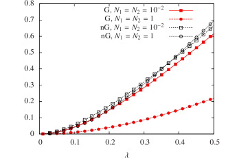
Figure 1: Gaussian and non-Gaussian quantum discord for STS as a function of $\lambda$, for different values of $N_{1}=N_{2}$

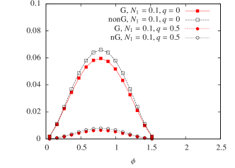
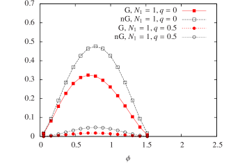
Figure 2: Gaussian and non-Gaussian quantum discord for MTS states as a function of $\phi$ for different values of $N_{1}$ and $q=N_{2}/N_{1}$

We have compared Gaussian and non-Gaussian quantum discord (with the non-Gaussian measurements corresponding to photon number measurements) for STS and MTS states with a wide range of squeezing, mixing and thermal parameters. In Fig. 1 we show results for STS with varying $\lambda$ and $N_{1}=N_{2}=10^{-2}$, $N_{1}=N_{2}=1$. The key result is that the non-Gaussian quantum discord is always greater than its Gaussian counterpart for all values of $N_{1}$ and $\lambda$. The gap grows with increasing $N_{1}$ and $\lambda$. In Fig. 2 we show results for MTS $N_{1}=\{0.1,1\}$ and $q=N_{2}/N_{1}=\{0,0.1,0.4,0.5\}$. Also in this case, the non-Gaussian discord is always higher than the Gaussian one.
Both results indicate that the Gaussian (heterodyne) measurement is optimal for STS and MTS states, at least compared to photon counting, in the sense that it allows for a better extraction of information on mode $A$ by a measurement on mode $B$.

V Squeezed Number basis

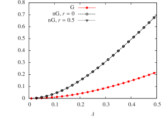
Figure 3: Gaussian and non-Gaussian quantum discord for STS with $N_{1}=1$ as a function of $\lambda$ and for different values of local squeezing $r$

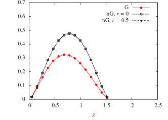
Figure 4: Gaussian and non-Gaussian quantum discord for MTS states for $N_{1}=1$, $N_{2}=0$ as a function of $\phi$ and for different values of local squeezing $r$

We now analyze the case of non-Gaussian measurements represented by the squeezed number basis $|n_{r}\rangle\!\langle n_{r}|=S(r)|n\rangle\!\langle n|S(r)^{\dagger}$, where $S(r)=\exp{(-r^{*}\frac{a^{2}}{2}-r\frac{(a^{\dagger})^{2}}{2})}$ is the single mode squeezing operator. A local measurement in the squeezed number basis is equivalent to a measurement in the number basis, performed on a locally squeezed state. In formulas, the probability of measuring $n_{r}$ on one subsystem when the state is the $\varrho$ is

$$p_{\varrho}(n_{r}) = \hbox{Tr}(\openone\otimes|n_{r}\rangle\!\langle n_{r}|\varrho)=\hbox{Tr}(\openone\otimes|n\rangle\!\langle n|S^{\dagger}(r)\varrho S(r))=$$ (19)

$$= \hbox{Tr}(\openone\otimes|n\rangle\!\langle n|\varrho^{r})=p_{\varrho_{r}}(n)$$

i.e., is equal to the probability of measuring $n$ on the locally squeezed state $\varrho_{r}=S(r)\varrho S(r)^{\dagger}$, and the relative post-measurement state is

$$\varrho_{n_{r}}^{A} = \hbox{Tr}_{B}[\openone\otimes|n_{r}\rangle\!\langle n_{r}|\varrho\openone\otimes|n_{r}\rangle\!\langle n_{r}|]/p_{\varrho}(n_{r})=$$ (20)

$$= \hbox{Tr}_{B}[\openone\otimes|n\rangle\!\langle n|\varrho_{r}\openone\otimes|n\rangle\!\langle n|]/p_{\varrho}^{r}(n)=\varrho_{r_{n}}^{A}$$

The general idea is that measurements on a state $\varrho$ in a basis that is obtained by performing a unitary (Gaussian) operation $V$ on the number basis $|n\rangle\!\langle n|$ can be represented as measurements on the number basis of a modified state $\varrho_{V}=V\varrho V^{\dagger}$ on which the local unitary operation acts.
In the case of the squeezed number basis, the post-measurement state is not diagonal, therefore the reasoning leading to Eq. (18) does not hold. The post-measurement state matrix elements $(\varrho_{r_{n}}^{A})_{h,k}=\varrho_{(h,k),(n,n)}$ can be obtained directly by evaluating the expression (16) where now the expression $O_{hk}(st)=\langle hk|O|st\rangle$ (where $O=S(\lambda),U(\phi)$) must be substituted with $O_{hk}^{\prime}(st)=\langle hk|S(r)O|st\rangle=\sum_{q}\langle k|S(r)|q\rangle\langle hq|O|st\rangle$, and the elements of the single mode squeezing operator are given in SingleModeSqueezing (eq. 20) or in SingleModeSqueezingKnight (eq. 5.1).
We have evaluated the Gaussian and non-Gaussian quantum discord for STS and MTS states with a wide range of two-mode squeezing and thermal parameters. Non-Gaussian measurements are done in the squeezed photon number basis, $\Pi_{n}=S(r)|n\rangle\langle n|S(r)^{\dagger}$ with variable $r\in[0,0.5]$. The effect of local squeezing on non-Gaussian quantum discord is negligible in the whole parameter range under consideration: we compare the non-Gaussian discord for different values of $r$ and find that all curves collapse. This can be seen in fig. 3 and fig. 4 where plot the behavior for $N_{1}=N_{2}=0.01$ (STS) and $N_{1}=1,N_{2}=0$ (MTS). The same behavior is observed in the whole parameter range under investigation. We have verified numerically that the post-measurement states of mode A $\varrho_{r_{n}}^{A}$ are not equal as $r$ varies (i.e., the post-measurement states corresponding to measurement result $n_{r}$ change with $r$), yet the sum $\sum_{n}p_{n}S(\varrho_{r_{n}}^{A})$ is equal for all values of $r$ under investigation. Therefore, the squeezing in the measurement basis has no effect on the discord, at least for the values of squeezing considered: in particular, it cannot afford a deeper minimization than that obtained without local squeezing. This indicates that the heterodyne measurement remains optimal also with respect to measurement in the squeezed number basis.

VI Displaced Number basis

We finally analyze the case of non-Gaussian measurements represented by the displaced number basis $|n_{\alpha}\rangle\!\langle n_{\alpha}|=D(\alpha)|n\rangle\!\langle n|D(\alpha)^{\dagger}$, where $D(\alpha)=\exp(\alpha a^{\dagger}-\alpha^{*}a)$ is the single mode displacement operator. According to the general considerations above, a local measurement in the displaced number basis is equivalent to a measurement in the number basis, performed on a locally displaced state $\varrho_{\alpha}$. As in the case of the squeezed number basis, the post-measurement state is not diagonal and we need all matrix elements $(\varrho_{\alpha_{n}}^{A})_{h,k}=\varrho_{(h,k),(n,n)}$. They can be obtained directly by evaluating the expression (16) where the expression $O_{hk}(st)=\langle hk|S(\lambda)|st\rangle$ (where $O=S(\lambda),U(\phi)$) must be substituted with $O_{hk}^{\prime}(st)=\langle hk|D(\alpha)O|st\rangle=\sum_{q}\langle k|D(\alpha)|q\rangle\langle hq|O|st\rangle$, and the elements of the single mode displacement operator are given in Parisbook (eq. 1.46).

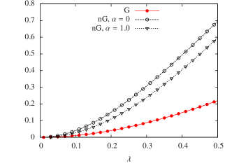
Figure 5: Gaussian and non-Gaussian quantum discord for STS with $N_{1}=1$ as a function of $\lambda$ and for different values of local displacement $\alpha$

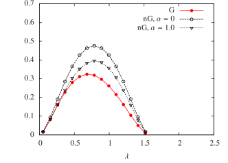
Figure 6: Gaussian and non-Gaussian quantum discord for MTS states for $N_{1}=1$, $N_{2}=0$ as a function of $\phi$ and for different values of local displacement $\alpha$

The evaluation of the non-Gaussian quantum discord can be simplified by first noticing that one can consider real values of $\alpha$ only. Indeed, the quantum discord only depends on the modulus $|\alpha|$. This is shown in detail in the appendix B, by using the characteristic function formalism. Consider $\varrho_{n_{\alpha}}^{A}$, the post-measurement state of mode $A$ after measurement result $n_{\alpha}$ is obtained on $B$. If we change the phase of $\alpha$, $\alpha\rightarrow\alpha^{\prime}\equiv e^{i\theta}\alpha$ we find that

$$\varrho_{n_{\alpha^{\prime}}}^{A}=U\varrho_{n_{\alpha}}^{A}U^{\dagger}$$ (21)

where $U$ is a unitary operation corresponding to a simple quadrature rotation

$$a_{1}\to a_{1}e^{i\theta}\quad a_{1}^{\dagger}\to a_{1}^{\dagger}e^{-i\theta}$$ (22)

Therefore, we have $\varrho_{\alpha^{\prime}_{n}}^{A}\neq\varrho_{\alpha_{n}}^{A}$, but $\varrho_{\alpha^{\prime}_{n}}^{A}$ and $\varrho_{\alpha_{n}}^{A}$ have the same spectrum, since they are related by a unitary. Therefore, the entropy of the reduced post-measurement state $\varrho_{\alpha}^{A}$ does not depend on the phase of $\alpha$ but just on $|\alpha|$. If follows that the non-Gaussian quantum discord of $\varrho_{\alpha}$ does not depend on the phase of $\alpha$.
We have evaluated the Gaussian and non-Gaussian quantum discord for STS and MTS states with a wide range of two-mode squeezing and thermal parameters. Non-Gaussian measurements are done in the displaced photon number basis, $\Pi_{n}=D(\alpha)|n\rangle\langle n|D(\alpha)^{\dagger}$ with variable $\alpha\in[0,2.5]$. In fig. 5 and fig. 6 we plot the Gaussian and non-Gaussian quantum discord. We see that greater displacements lead to lower values of the non-Gaussian quantum discord, but the decrease is insufficient to match the Gaussian quantum discord, which remains optimal. However, the non-Gaussian quantum discord approximates the Gaussian one as $\alpha\to\infty$. This is analytically proven below in the appendix C. There we find that for both STS and MTS

$$\varrho_{\alpha_{n}}^{A}\to\varrho_{\alpha_{0}}^{A}\qquad\mbox{as}\quad\alpha\to\infty$$ (23)

i.e, the conditional states $\varrho_{\alpha_{n}}^{A}$ becomes independent of $n$ and equal to the $n=0$ result. As a consequence, the conditional entropy in the displaced number basis is equal to the entropy of the post-measurement state for any measurement result, and, in particular, for $n=0$:

$$S^{\Pi,\mathcal{NG}}(A|B)=\sum_{n}p_{n}S(\varrho_{\alpha_{n}}^{A})\to S(\varrho_{\alpha_{0}}^{A})\quad\mbox{as}\quad\alpha\to\infty$$ (24)

But $\varrho_{\alpha_{0}}^{A}$ is just the post-measurement state we obtain after a heterodyne detection on mode $B$ (equal for all measurement result modulo a phase space translation which is irrelevant as for the entropy). Therefore, we also have $S^{G}(A|B)=S(\varrho_{\alpha_{0}}^{A})$ and the non Gaussian discord $D^{\mathcal{NG}}(A:B)$ in the displaced number basis tends to the Gaussian discord $D^{\mathcal{G}}(A:B)$ as $\alpha\to\infty$.

Actually, we cannot prove that the $D^{\mathcal{NG}}(A:B)$ is lower bounded by $D^{\mathcal{G}}(A:B)$, and we cannot rule out the possibility that $D^{\mathcal{NG}}(A:B)<D^{\mathcal{G}}(A:B)$ for intermediate values of $\alpha$. However, our numerical data do not support this possibility since we never observe $D^{\mathcal{NG}}(A:B)<D^{\mathcal{G}}(A:B)$ and we expect that $D^{\mathcal{NG}}(A:B)\to D^{\mathcal{G}}(A:B)$ from above as $\alpha\to\infty$.
In conclusion, we have analytical and numerical evidence that the heterodyne measurement remains optimal also with respect to measurement in the displaced number basis.

VII Geometric discord

In this section, we briefly consider the recently introduced measure of geometric discord and compare results with those obtained for the quantum discord. The geometric discord Dakic is defined as

$$D_{G}(A:B)=\min_{\{\chi_{AB}\in\mathcal{C}\}}||\varrho_{AB}-\chi_{AB}||_{2}$$ (25)

and it measures the distance of a state from the set $\mathcal{C}$ of quantum-classical states where $||A||_{2}=\mbox{Tr}[A^{\dagger}A]$ is the Hilbert-Schmidt distance. Clearly $D_{G}=0$ iff $D=0$, since both measures vanish on the set of classically correlated states. In particular, it has been be proven that $D_{G}$ can be seen a measure of the discrepancy between a state before and after a local measurement on subsystem $B$ Luo :

$$D_{G}(A:B)=\min_{\{\Pi\in POVM\}}||\varrho_{AB}-\varrho_{AB}^{\Pi}||_{2}$$ (26)

where the unconditional post-measurement state is given by $\varrho_{AB}^{\Pi}=\sum_{x}M_{B}^{x}\varrho_{AB}M_{B}^{x{\dagger}}$. Notice that $D_{G}$ and $D$ are not monotonic functions of one another and the relation between them is still an open question. However, in many cases $D_{G}$ is much simpler to evaluate than $D$.

Analogous to the case of Gaussian discord, a Gaussian version of the geometric discord can be defined by restricting to Gaussian measurements GaussianGeom . Again, it can be analytically computed for two-mode Gaussian states. With the same reasoning of sec. II one easily obtains

$$D_{G}^{\mathcal{G}}(\varrho_{AB})=\mbox{min}_{\sigma_{M}}\mbox{Tr}[(\varrho_{AB}-\varrho_{P}\otimes\varrho_{M})^{2}]$$ (27)

Exploiting the property that $\mbox{Tr}[\varrho_{1}\varrho_{2}]=1/\det[(\sigma_{1}+\sigma_{2})/2],$ for any two Gaussian states $\varrho_{1}$ and $\varrho_{2}$,

$$D_{G}(A:B)=\mbox{min}_{\sigma_{M}}\{1/\sqrt{\det\sigma_{AB}}+$$ (28)

$$+1/\sqrt{\det(\sigma_{P}\oplus\sigma_{M})}-2/\sqrt{\det[(\sigma_{AB}+\sigma_{P}\oplus\sigma_{M})/2]}\}$$

For for the relevant case of STS and MTS, the minimum is obtained with the $\sigma_{M}$ elements given by $\alpha=\beta=\frac{\sqrt{ab}(\sqrt{4ab-3c^{2}}+\sqrt{ab})}{3a}$, $\gamma=0$. The least disturbing Gaussian POVM for STS, according to the Hilbert-Schmidt distance, is thus a (noisy) heterodyne detection, a result which is analogous to what found in the case of quantum discord. If one constrains the mean energy per mode, the Gaussian quantum discord gives upper and lower bounds to the Gaussian geometric discord. In absence of such a provision, the geometric discord can vanish for arbitrarily strongly nonclassical (entangled) Gaussian states, as a consequence of the geometry of CV state spaces.

Also in this case, we may consider non-Gaussian measurements and evaluate a non-Gaussian geometric discord:

$$D_{G}^{\mathcal{NG}}(A:B)=\mbox{Tr}[(\varrho_{AB}-\varrho_{AB}^{\Pi})^{2}]$$ (29)

For measurement in the number basis, we can easily obtain

$$D_{G}^{\mathcal{NG}}=\mu(\varrho)+\sum_{npq}|\langle pn|\varrho|qn\rangle|^{2}$$ (30)

where $\mu(\varrho)=\frac{1}{4\sqrt{\det(\sigma)}}$ is the (Gaussian) state purity Parisbook . In the case of measurements in the squeezed or displaced number basis, we have to use $\varrho_{r}$ and $\varrho_{\alpha}$ instead of $\varrho$ in Eq. (30). In general, in order to compute the geometric discord we need to compute matrix elements, and we use the same numerical methods described above.

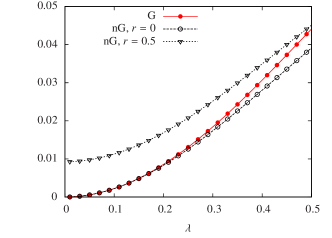
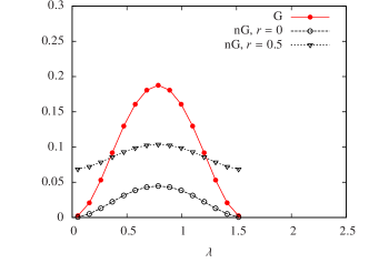
Figure 7: (Top) Gaussian and non-Gaussian geometric discord for STS with $N_{1}=1$ as a function of $\lambda$ and for different values of local squeezing $r$; (Bottom) Gaussian and non-Gaussian geometric discord for MTS states for $N_{1}=1$, $N_{2}=0$ as a function of $\phi$ and for different values of local squeezing $r$

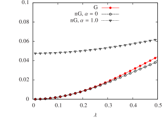
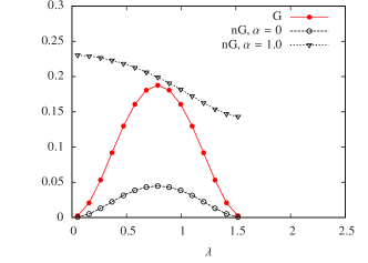
Figure 8: (Top) Gaussian and non-Gaussian geometric discord for STS with $N_{1}=1$ as a function of $\lambda$ and for different values of local displacement $\alpha$ (Bottom) Gaussian and non-Gaussian geometric discord for MTS states for $N_{1}=1$, $N_{2}=0$ as a function of $\phi$ and for different values of local displacement $\alpha$

VII.1 Results

. We have compared the Gaussian and non-Gaussian geometric discord for STS and MTS in a wide range of parameters. We have considered measurements in the number, squeezed number and displaced number basis for the same values of the parameters given in the preceding sections. Results are plotted in Figs. 7 and 8. In general, at variance with the results for quantum discord, we find that non-Gaussian measurements can provide lower values of geometric discord than Gaussian ones. Among the class of non-Gaussian measurements we have considered, the optimal one is provided by the number basis, which gives values of geometric discord that are always lower than those given by the optimal Gaussian measurement. The non-Gaussian geometric discord increases for increasing $r$ and $\alpha$, and it can become greater than its Gaussian counterpart. These results are very different from the quantum discord case: on one hand, the (non-Gaussian) geometric discord is substantially affected by the local squeezing; on the other hand, it does not approach the Gaussian one when the displacement $\alpha\to\infty$, but it grows monotonically. Indeed if we increase the squeezing or displacement in the measurement basis, the post-measurement state is more distant (in Hilbert-Schmidt norm) from the original one. As already noticed, performing the measurement is the squeezed (displaced) number basis in equivalent to first squeezing (displacing) the state and then measuring it in the number basis. The local squeezing and displacement have the effect of increasing the energy of the state, shifting the photon number distribution $P(B=n)$ towards greater values of $n$. This causes the overlap between the post measurement state and the original state to decrease, and therefore their distance to increase.

Let us futher comment on the difference between the quantum discord and the geometric discord cases. Quantum discord and geometric discord both vanish for classical states, but are not monotonic functions of one another, and thus they are truly different quantities. The geometric discord, based on the Hilbert-Schmidt distance, is a geometric measure of how much a state is perturbed by a local measurement, while quantum discord assesses to which extent correlations are affected by a local measurement. While for the quantum discord well-defined operational and informational interpretations can be found Gu ; Datta2 , for the geometric discord the situation is more problematic. Indeed, one can design protocols in which the geometric discord can in some cases be related to the protocols’ performances RSP ; Tufarelli ; however, recent discussions  Piani , show that, as consequence of the noninvariance of the Hilbert-Schmidt norm under quantum evolutions, it is difficult to find a conclusive argument about the relevance of geometric discord as a measure of quantumness of correlations. Our data show that non-Gaussian measurements can yield optimal values of the geometric discord, contrary to the case of quantum discord. Hence, the behavior of quantum discord and geometric discord with respect to different types of measurements is different. This is a further indication that the geometric discord cannot be used as a good benchmark for the quantum discord and that the degree of quantumness measured, if any, by such a quantity has a fundamentally different nature.

VIII Discussion and conclusions

The definition of discord involves an optimization over all possible local measurements (POVMs) on one of the subsystems of a bipartite composite quantum system. In the realm of continuous variables (CV), initial research efforts on quantum discord restricted the minimization to the set of (one-mode) Gaussian measurements.

In this work we have investigated CV quantum discord beyond this restriction. We have focused on Gaussian states, asking whether Gaussian measurements are optimal in this case, i.e., whether the Gaussian discord is the true discord for Gaussian states. While a positive answer to this question had already been given for the special case of two-mode Gaussian states having one vacuum normal mode (by means of an analytical argument based on the Koashi-Winter formula), no general result was available so far. We have addressed our central question upon considering two large classes of two-mode Gaussian states, the squeezed thermal states (STS) and the mixed thermal states (MTS), and allowing for a wide range of experimentally feasible non-Gaussian measurements based on orthogonal bases: the photon number basis, the squeezed number basis, the displaced number basis. For both STS and MTS states, in the range of parameters considered, the Gaussian measurements always provide optimal values of discord compared to the non-Gaussian measurements under analysis. Local squeezing of the measurement basis has no appreciable effect on correlations, while local displacement leads to lower values of the non-Gaussian discord, which approaches the Gaussian one in the limit of infinite displacement.

Overall, for the explored range of states and measurements, we have evidence that the Gaussian discord is the ultimate quantum discord for Gaussian states. We note that the optimality of Gaussian measurements suggested by our analysis is a property which holds only for Gaussian states. In the case of non-Gaussian states, e.g., CV Werner states, non-Gaussian measurements such as photon counting can lead to a better minimization, as was recently proven in Ref. NonGausDisc .

We also have investigated the CV geometric discord GaussianGeom , comparing the Gaussian and non-Gaussian cases. We have shown that the behavior of geometric discord is completely different from that of quantum discord. On one hand, non-Gaussian measurements can lead to lower values of the geometric discord, the number basis measurement being the optimal one; on the other hand, the effects of both local squeezing and displacement are strong and consist in a noteworthy increase in the non-Gaussian geometric discord. The remarkable differences between quantum and geometric discord imply that the latter cannot be used as a benchmark of the former.

Both in the case of the discord and geometric discord a definite answer on the optimal measurement minimizing the respective formulas would require the extension of the set of non-Gaussian measurements to possibly more exotic ones and the application of those realizable in actual experiments to a broader class of Gaussian and non-Gaussian states. While we leave this task for future research, our results on discord support the conjecture that Gaussian measurements are optimal for Gaussian states and allow to set, for the class of states analyzed, a tighter upper bound on the entanglement of formation for $1\times 2$ modes Gaussian states, via the Koashi-Winter relation.

Appendix A The post-measurement state is diagonal

We prove that the post-measurement state

$$\varrho_{n}^{A}=\hbox{Tr}_{B}[\openone\otimes|n\rangle\!\langle n|\ \varrho\ \openone\otimes|n\rangle\!\langle n|]/p_{n}$$ (31)

of STS and MTS after local measurement in the number basis is diagonal (here, $p_{n}=\hbox{Tr}[\varrho\openone\otimes|n\rangle\!\langle n|]$). We have indeed:

$$\varrho=\sum_{s,t}p^{th}_{s}(N_{1})p^{th}_{t}(N_{2})O|st\rangle\!\langle st|O^{\dagger}=$$

$$=\sum_{(h,n),(k,m)}|hn\rangle\!\langle km|\left(\sum_{s,t}p^{th}_{s}p^{th}_{t}O_{hn}(st)O_{km}^{*}(st)\right)$$ (32)

where $p^{th}_{s}(N)=N^{s}\ (1+N)^{-(s+1)}$ where $O_{hn}(st)=\langle hn|O|st\rangle$ and $O_{km}^{*}(st)=\langle st|O^{\dagger}|km\rangle=\langle km|O|st\rangle^{*}$, where $O=S(\lambda)$, $O=U(\phi)$ for STS and MTS respectively. The post measurement states can be written as:

$$\varrho^{A}_{n}\otimes|n\rangle\!\langle n|=\left(\sum_{h,k}\varrho_{(h,k),(n,n)}|h\rangle\!\langle k|\right)\otimes|n\rangle\!\langle n|$$ (33)

and therefore we need to evaluate the matrix elements

$$\varrho_{(h,k),(n,n)}=\sum_{s,t}p^{th}_{s}p^{th}_{t}O_{hn}(st)O_{kn}^{*}(st)$$ (34)

The elements of the two-mode squeezing operator are given in SNS4 (eq. 22):

$$\langle hn|S(\lambda)|st\rangle=\delta_{t+h,s+n}f^{\lambda}(h,n,s,t)=\delta_{t+h,s+n}\times$$

$$\sum_{a=0}^{min(s,t)}\sum_{b=0}^{min(h,n)}(-1)^{a+b}(sech\lambda)^{t+h-a-b-1}\mu^{a-b+h-s}\times$$

$$\frac{(t+h-a-b)![s!t!h!n!]^{1/2}}{a!(t-a)!(s-a)!b!(n-b)!(h-b)!}\qquad\qquad$$ (35)

where $\mu=e^{\lambda}$, while the elements of the two-mode mixing operator

$$\langle hn|U(\phi)|st\rangle=\delta_{h+n,s+t}\sum_{a=\max\{0,h-t\}}^{\min\{h,s\}}A_{a\ h-a}^{s\ t}$$

$$=\delta_{h+n,s+t}\sum_{a=\max\{0,h-t\}}^{\min\{h,s\}}\sqrt{\frac{h!(s+t-h)!}{s!t!}}(-1)^{h-a}\times$$

$$\binom{s}{a}\binom{t}{h-a}\sin\phi^{s+h-2a}\cos\phi^{t+2a-h}\qquad\qquad$$ (36)

In order to evaluate (34), we need $O_{hn}(st)O_{kn}^{*}(st)$. Due to the $\delta$’s appearing in both (35) and (36), the following relations must be satisfied:

$$t-s = n-h$$

$$t-s = n-k.$$

and this implies $h=k$; therefore the post-measurement state is diagonal in the number basis:

$$(\varrho_{n}^{A})_{h,k}=\delta_{h,k}\sum_{s,t}p^{th}_{s}(N_{1})p^{th}_{t}(N_{2})|O_{hk}(st)|^{2}$$ (37)

Appendix B Discord does not depend on the phase of displacement

We show that the (non-Gaussian) discord in the displaced number basis does not depend on the phase of displacement for STS and MTS. The arguments is best given in the characteristic function representation of the states citeParisbook The STS and MTS states have a Gaussian characteristic function $\chi[\varrho](\mathbf{\Lambda})=\exp(-\frac{1}{2}\mathbf{\Lambda}^{T}\sigma\mathbf{\Lambda})$ where $\mathbf{\Lambda}=\frac{1}{\sqrt{2}}(\mbox{Re}\lambda_{A},\mbox{Im}\lambda_{A},\mbox{Re}\lambda_{B},\mbox{Im}\lambda_{B})$ and the covariance matrix is given by

$$\sigma=\left(\begin{array}[]{cc}A&C\\ C^{T}&B\end{array}\right)=\left(\begin{array}[]{cccc}a&0&c&0\\ 0&a&0&\pm c\\ c&0&b&0\\ 0&\pm c&0&b\end{array}\right)$$ (38)

where $\pm c$ is $-c$ in the case of STS and $+c$ in the case of MTS. For STS we have

$$\chi[\varrho](\lambda_{A},\lambda_{B})=\exp(-a|\lambda_{A}|^{2}-b|\lambda_{B}|^{2}+2c\mbox{Re}[\lambda_{A}\lambda_{B}])$$ (39)

while for MTS the same expression holds upon changing $2c\mbox{Re}[\lambda_{A}\lambda_{B}]\to 2c\mbox{Re}[\lambda_{A}^{*}\lambda_{B}]$. In the following, we shall carry on the argument for STS, but the MTS case is fully equivalent. If we perform a displacement on one mode, $\varrho\rightarrow D(\alpha)\varrho D^{\dagger}(\alpha)\equiv\varrho_{\alpha}$, the effect on the characteristic function is easy to evaluate. Using the relation $D(\alpha)D(\lambda)D^{\dagger}(\alpha)=D(\lambda)\exp(-2i\mbox{Im}[\lambda\alpha^{*}])$ Parisbook we obtain

$$\chi[\varrho_{\alpha}](\lambda_{A},\lambda_{B})=\chi[\varrho](\lambda_{A},\lambda_{B})\exp(-2i\mbox{Im}[\lambda_{B}\alpha^{*}])$$ (40)

Suppose we perform a masurement on mode $B$ in the number basis $\{\Pi_{n}=|n\rangle\langle n|\}$. The post-measurement state of mode $A$ is $\varrho_{\alpha,n}^{A}=\frac{1}{p_{n}}\mbox{Tr}_{B}[\varrho_{\alpha}\Pi_{n}]$ where $p_{n}=\mbox{Tr}[\varrho_{\alpha}\Pi_{n}]$. By use of the trace formula Parisbook

$$\mbox{Tr}[O_{1}O_{2}]=\frac{1}{\pi}\int_{\mathbb{C}^{m}}d^{2m}\lambda\ \chi[O_{1}](\lambda)\chi[O_{2}](-\lambda)$$

we obtain the characteristic function

$$\chi[\varrho_{\alpha_{n}}^{A}](\lambda_{A})=\frac{1}{\pi p_{n}}\int_{\mathbb{C}}d^{2}\lambda_{B}\ \chi[\Pi_{n}](\lambda_{B})\ \chi[\varrho_{\alpha}](\lambda_{A},-\lambda_{B})$$ (41)

Since $\chi[\Pi_{n}](\lambda_{B})=e^{-\frac{1}{2}|\lambda_{B}|^{2}}L_{n}(|\lambda_{B}|^{2})$, where $L_{n}$ is the Laguerre polynomial $L_{n}(|\lambda_{B}|^{2})=\sum_{i=0}^{n}\binom{n}{n-i}\frac{|\lambda_{B}|^{2i}}{i!}$, we have explicitly

$$\chi[\varrho_{\alpha_{n}}^{A}](\lambda_{A})=\frac{1}{\pi p_{n}}\int_{\mathbb{C}}d^{2}\lambda_{B}\ L_{n}(|\lambda_{B}|^{2})\exp\left(-a|\lambda_{A}|^{2}\right.$$

$$\left.-(b+1/2)|\lambda_{B}|^{2}-2c\mbox{Re}[\lambda_{A}\lambda_{B}]-2i\mbox{Im}[\lambda_{B}\alpha^{*}]\right)$$

(42)

In order to see that this expression depends on $|\alpha|$ only we can implement the change $\alpha\rightarrow\alpha^{\prime}\equiv e^{i\theta}\alpha$ and we have

$$\chi[\varrho_{\alpha_{n}^{\prime}}^{A}](\lambda_{A})=\frac{1}{\pi p_{n}}\int_{\mathbb{C}}d^{2}\lambda_{B}\quad L_{n}(|\lambda_{B}|^{2})\exp\left(-a|\lambda_{A}|^{2}\right.$$

$$\left.-(b+1/2)|\lambda_{B}|^{2}-2c\mbox{Re}[\lambda_{A}\lambda_{B}]-2i\mbox{Im}[\lambda_{B}\alpha^{*}e^{-i\theta}]\right)$$

By changing variable $\lambda_{B}\to e^{-i\theta}\lambda_{B}$ we see that

$$\chi[\varrho_{\alpha_{n}^{\prime}}^{A}](\lambda_{A})=\chi[\varrho_{\alpha_{n}}^{A}](\lambda_{A}e^{-i\theta})$$ (43)

Therefore, we have $\chi[\varrho_{\alpha_{n}^{\prime}}^{A}]\neq\chi[\varrho_{\alpha_{n}}^{A}]$, hence $\varrho_{\alpha_{n}^{\prime}}^{A}\neq\varrho_{\alpha_{n}}^{A}$. However, $\varrho_{\alpha_{n}^{\prime}}^{A}$ and $\varrho_{\alpha_{n}}^{A}$ have the same spectrum. Indeed $\chi[\varrho_{\alpha_{n}}^{A}(\lambda_{A})]$ and $\chi[\varrho_{\alpha_{n}}^{A}(\lambda_{A}e^{i\theta})]$ are related by a simple quadrature rotation

$$a_{1}\to a_{1}e^{i\theta}\quad a_{1}^{\dagger}\to a_{1}^{\dagger}e^{-i\theta}$$ (44)

which means that

$$\varrho_{\alpha_{n}^{\prime}}^{A}=U\varrho_{\alpha_{n}}^{A}U^{\dagger}$$ (45)

where $U$ is the free evolution of mode $A$, $U=e^{i\theta a_{1}^{\dagger}a_{1}}$. Since $\varrho_{\alpha_{n}^{\prime}}^{A}$ and $\varrho_{\alpha_{n}}^{A}$ are related by a unitary, they have the same spectrum. Therefore, the spectrum (hence, the entropy) of the reduced post-measurement state $\varrho_{\alpha}^{A}$ does not depend on the phase of $\alpha$ but just on $|\alpha|$. If follows that the non-Gaussian quantum discord of $\varrho_{\alpha}$ does not depend on the phase of $\alpha$, QED.
As for the non-Gaussian geometric discord, it is obtained as

$$\mbox{Tr}[(\varrho)^{2}]-\sum_{n}\mbox{Tr}[\varrho_{\alpha_{n}}^{A}\varrho_{\alpha_{n}}^{A}\otimes\Pi_{n}^{B}]=$$

$$=\mbox{Tr}[(\varrho)^{2}]-\sum_{n}\mbox{Tr}[\varrho_{\alpha_{n}}^{A}\varrho_{\alpha_{n}}^{A}]$$

By the same arguments before, leading to eq. (45), we immediately see that the second trace does not depend on the phase of $\alpha$, hence the geometric discord does neither.

Appendix C Understanding the behavior for growing $\alpha$

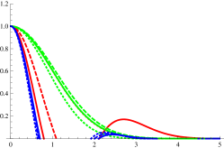
(a) Re

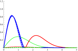
(b) Im

Figure 9: $\chi[\varrho_{\alpha_{n}^{A}}](\lambda)$ for $\alpha=0.1$ (red), $\alpha=1$ (green), $\alpha=5$ (blue) and $n=0$ (solid), $n=1$ (dashed), $n=2$ (dotted). Here, we have $A=(N_{T}+1/2)\cosh\lambda$, $C=(N_{T}+1/2)\sinh\lambda$ with $\lambda=0.5$, $N_{T}=0.5$.

Let us now consider in detail the bahaviour for growing $\alpha$. We will show that the non-Gaussian discord in the displaced number basis tends to the Gaussian discord as the displacement tends to infinity, $D^{\mathcal{NG}}\to D^{\mathcal{G}}$ as $\alpha\to\infty$.
First, we will show that

$$\varrho_{\alpha_{n}}^{A}\to\varrho_{\alpha_{0}}^{A}\quad\mbox{as}\quad\alpha\to\infty$$ (46)

This is best shown in the characteristic function formalism. The post-measurement state of mode $A$ has the characteristic function (42). Since the phase of $\alpha$ is irrelevant for the discord, we will assume $\alpha\in\mathbb{R}$ in the following. The post-measurement state characteristic function, Eq. (42), is the Gaussian integral of a polynomial. By using a well-known trick of Gaussian integrals, we can rewrite

$$\chi[\varrho_{\alpha_{n}}^{A}](\lambda_{A})=\frac{1}{\pi p_{n}}e^{-a|\lambda_{A}|^{2}}\int_{\mathbb{C}}d^{2}\lambda_{B}\quad L_{n}(d/d\gamma)\times$$

$$\exp\left(-\gamma|\lambda_{B}|^{2}+2c\mbox{Re}\lambda_{A}\mbox{Re}\lambda_{B}-(2c\mbox{Im}[\lambda_{A}]+2i\alpha)\mbox{Im}[\lambda_{B}]\right)$$

where $\gamma=b+1/2$ and the formal expression $L_{n}(d/d\gamma)$ means $\sum_{i=0}^{n}\binom{n}{n-i}\frac{1}{i!}\frac{d^{n}}{d\gamma^{n}}$. This expression can now be moved outside the integral, so that we are now left with a purely Gaussian integral of the form

$$\int_{\mathbb{R}}d^{2}\mathbf{\Lambda}_{B}\ e^{-\frac{1}{2}\mathbf{\Lambda}_{B}^{T}\mathcal{M}\mathbf{\Lambda}_{B}+\mathbf{\Lambda}_{B}^{T}\mathcal{B}}$$

where $\mathcal{M}=\mbox{diag}\{4\gamma,4\gamma\}$, $\mathcal{B}=(2c\mbox{Re}\lambda_{A},-2c\mbox{Im}\lambda_{A}+2i\alpha)$, $\mathbf{\Lambda_{B}}=(\mbox{Re}\lambda_{B},\mbox{Im}\lambda_{B})$. The integral gives $\frac{2\pi}{\sqrt{\mbox{det}\mathcal{M}}}e^{\frac{1}{2}\mathcal{B}^{T}\mathcal{M}^{-1}\mathcal{B}}$ so that we finally get

$$\chi[\varrho_{\alpha_{n}}^{A}](\lambda_{A})=\frac{1}{p_{n}}e^{-\frac{1}{2}a|\lambda_{A}|^{2}}L_{n}(-d/d\gamma)\times$$ (47)

$$\frac{1}{\gamma}\exp\left(\frac{c^{2}|\lambda_{A}|^{2}-\alpha^{2}-2i\alpha c\mbox{Im}\lambda_{A}}{2\gamma}\right)$$

Let us define $x=c^{2}|\lambda_{A}|^{2}-\alpha^{2}-2i\alpha c\mbox{Im}\lambda_{A}$. Then we have

$$L_{n}(-d/d\gamma)\frac{1}{\gamma}\exp\left(\frac{c^{2}|\lambda_{A}|^{2}-\alpha^{2}-2i\alpha c\mbox{Im}\lambda_{A}}{2\gamma}\right) =$$

$$=L_{n}(-d/d\gamma)\frac{1}{\gamma}e^{x/2\gamma}=F_{n}(\gamma,x)e^{x/2\gamma}$$

where $F_{n}(\gamma,x)=\sum_{k}f_{k}(\gamma)x^{k}$ is necessarily a polynomial of degree $n$ in with $\gamma$-dependent coefficients $f_{k}(\gamma)$. Therefore,

$$\chi[\varrho_{\alpha_{n}}^{A}](\lambda_{A})=\frac{1}{p_{n}}e^{-(a-c^{2}(b+1/2)^{-1})|\lambda_{A}|^{2}}\times$$ (48)

$$e^{-ic(b+1/2)^{-1}\alpha Im\lambda_{A}}e^{-\alpha^{2}/2\gamma}F_{n}(\gamma,x)$$

The norm is

$$p_{n}=e^{-(a-c^{2}(b+1/2)^{-1})|\lambda_{A}|^{2}}e^{-ic(b+1/2)^{-1}\alpha Im\lambda_{A}}\times$$

$$e^{-\alpha^{2}/2\gamma}F_{n}(\gamma,x)\Big{|}_{\lambda_{A}=0}=e^{-\alpha^{2}/2\gamma}F_{n}(-\alpha^{2})$$

so that

$$\chi[\varrho_{\alpha_{n}}^{A}](\lambda_{A})=e^{-(a-c^{2}(b+1/2)^{-1})|\lambda_{A}|^{2}}\times$$ (49)

$$e^{-ic(b+1/2)^{-1}\alpha Im\lambda_{A}}\frac{F_{n}(\gamma,x)}{F_{n}(\gamma,-\alpha^{2})}$$

This function is exponentially decaying as $e^{-s|\lambda_{A}|^{2}}$ where $s=a-c^{2}/(b+1/2)$, hence it is vanishing for $|\lambda_{A}|^{2}\gg 1/s$. Therefore, we can consider values of $|\lambda_{A}|^{2}$ in the region $\lambda_{A}^{2}\lesssim 1/s$. In this region, we we have $\lim_{\alpha\to\infty}x=-\alpha^{2}$ because $\alpha\gg\lambda_{A}$ and thus

$$\lim_{\alpha\to\infty}\frac{F_{n}(\gamma,x)}{F_{n}(\gamma,-\alpha^{2})}=\frac{f_{n}(\gamma)\alpha^{2}n}{f_{n}(\gamma)\alpha^{2}n}=1$$

In conclusion, as $\alpha\to\infty$ we have

$$\chi[\varrho_{\alpha_{n}}^{A}](\lambda_{A})\to\chi[\varrho_{\alpha_{0}}^{A}]$$ (50)

which implies the desired result (46), QED.

This result means that the conditional state of $A$ is independent of $n$ and equal to the $n=0$ result. In fig. 9 we show $\chi[\varrho_{\alpha_{0}}^{A}],\chi[\varrho_{\alpha_{1}}^{A}],\chi[\varrho_{\alpha_{2}}^{A}]$ for growing values of $\alpha$. The three curves converge already for $\alpha\sim 5$. As a consequence of $n$-independence, we have

$$S^{\Pi,\mathcal{NG}}(A|B)=\sum_{n}p_{n}S(\varrho_{\alpha_{n}}^{A})\to S(\varrho_{\alpha_{0}}^{A})$$ (51)

But $\varrho_{\alpha_{0}}^{A}$ is just the post-measurement state corresponding to POVM element $D(\alpha)|0\rangle\langle 0|D^{\dagger}(\alpha)=|\alpha\rangle\langle\alpha|$, i.e, a Gaussian state with covariance matrix $\sigma_{P}=A-C(B+\mathbb{I}/2)^{-1}C^{T}$ (Schur complement), and mean $\mu_{P}=X(B+\mathbb{I}/2)^{-1}C^{T}$, where $X=(\alpha,0)$. On the other hand, from the discussion in sec. II we know that the optimal Gaussian POVM is a heterodyne measurement $\{\Pi_{\beta}=D(\beta)|0\rangle\langle 0|D^{\dagger}(\beta)=|\beta\rangle\langle\beta|\}$. In this case, as already explained in sec. II, the entropy of the post measurement state $\varrho_{\beta}^{A}$ is independent of the measurement result $\beta$, hence the conditional entropy coincides with the entropy of of the $\beta=\alpha$ result. Therefore, we also have $S^{\mathcal{G}}(A|B)=S(\varrho_{\alpha_{0}})$. Therefore, we conclude that the non Gaussian discord $D^{\mathcal{NG}}(A:B)$ in the displaced number basis tends to the Gaussian discord $D^{\mathcal{G}}(A:B)$ as $\alpha\to\infty$, QED.
To be rigorous, we did not prove that the $D^{\mathcal{NG}}(A:B)$ is lower bounded by $D^{\mathcal{G}}(A:B)$, and we cannot rule out the possibility that $D^{\mathcal{NG}}(A:B)<D^{\mathcal{G}}(A:B)$ for intermediate values of $\alpha$. However, our numerical data do not support this possibility since we never observe $D^{\mathcal{NG}}(A:B)<D^{\mathcal{G}}(A:B)$ and we expect that $D^{\mathcal{NG}}(A:B)\to D^{\mathcal{G}}(A:B)$ from above as $\alpha\to\infty$.

References

- (1) R. Horodecki, P. Horodecki, M. Horodecki, and K. Horodecki, Rev. Mod. Phys. 81, 865 (2009).
- (2) H. Ollivier and W. H. Zurek, Phys. Rev. Lett. 88, 017901 (2001).
- (3) L. Henderson and V. Vedral, J. Phys. A 34, 6899 (2001).
- (4) K. Modi, A. Brodutch, H. Cable, T. Paterek and V. Vedral, arXiv:1112.6238 (2011).
- (5) M. Gu, H. M. Chrzanowski, S. M. Assad, T. Symul, K. Modi, T. C. Ralph, V. Vedral, P. K. Lam, arXiv:1203.0011 (2012).
- (6) V. Madhok, A. Datta, arXiv:1204.6042 (2012).
- (7) A. Datta, A. Shaji, and C. M. Caves, Phys. Rev. Lett. 100, 050502 (2008); A. Datta and A. Shaji, Int. J. Quant. Inf. 9, 1787 (2011); A. Brodutch and D. R. Terno, Phys. Rev. A 83, 010301 (2011); A. Al-Qasimi and D. F. V. James, Phys. Rev. A 83, 032101 (2011); G. Passante, O. Moussa, D. A. Trottier, R. Laflamme, Phys. Rev. A. 84, 044302 (2011) (2011).
- (8) B. Dakić et al., arXiv:1203.1629 (2012).
- (9) A. Ferraro, M. G. A. Paris, arXiv:1203.2661 (2012).
- (10) B. Dakić, C. Brukner, and V. Vedral, Phys. Rev. Lett. 105, 190502 (2010).
- (11) S. Luo, Phys. Rev. A 77, 042303 (2008); M. Ali, A. R. P. Rau, and G. Alber, Phys. Rev. A 81, 042105 (2010).
- (12) P. Giorda and M. G. A. Paris, Phys. Rev. Lett. 105, 020503 (2010).
- (13) G. Adesso and A. Datta, Phys. Rev. Lett. 105, 030501 (2010).
- (14) G. Giedke and J. I. Cirac, Phys. Rev. A 66, 032316 (2002); J. Fiuràšek and L. Mišta Jr., Phys. Rev. A (75, 060302(R) 2007).
- (15) R. Vasile, P. Giorda, S. Olivares, M. G. A. Paris, and S. Maniscalco, Phys. Rev. A 82, 012313 (2010); G. L. Giorgi, F. Galve, R. Zambrini, Int. J. Quant. Inf. 9, 1825 (2011); L. A. Correa, A. A. Valido, D. Alonso. arXiv:1111.0806v2 (2011).
- (16) G. L. Giorgi, F. Galve, G. Manzano, P. Colet, R. Zambrini, Phys. Rev. A 85, 052101 (2012).
- (17) R. Tatham, L. Mišta Jr., G. Adesso, N. Korolkova, Phys. Rev. A 85, 022326 (2012).
- (18) M. Koashi and A. Winter, Phys. Rev. A 69, 022309 (2004).
- (19) G. Adesso and D. Girolami, Int. J. Quant. Inf. 9 (2011).
- (20) G. Giedke, M. M. Wolf, O. Krüger, R. F. Werner, and J. I. Cirac, Phys. Rev. Lett. 91, 107901 (2003); J. Solomon Ivan, R. Simon, arXiv:0808.1658; P. Marian, T. A. Marian, Phys. Rev. Lett. 101, 220403 (2008).
- (21) M. G. A. Paris, Phys. Lett. A 217, 78 (1996).
- (22) F. A. M. de Oliveira, M. S. Kim, P. L. Knight, abd V. Bužek, Phys. Rev. A 41, 2645 (1990).
- (23) H. P. Yuen, J. Opt. Soc. Am B 3, P86 (1986).
- (24) M. S. Kim, F. A. M. de Oliveira, and P. L. Knight, Phys. Rev. A 40, 2494 (1989).
- (25) R. T. Hammond, Phys. Rev. A 41, 1718 (1990).
- (26) C. F. Lo , Phys. Rev. A 43, 404 (1991); M. M. Nieto, Phys. Lett. A 229, 135 (1997).
- (27) C. T. Lee, Phys. Rev. A 42, 4193 (1990).
- (28) A. Furusawa, J. L. Sorensen, S. L. Braunstein, C. A. Fuchs, H. J. Kimble, and E. S. Polzik, Science 282, 706 (1998); N. Lee, H. Benichi, Y. Takeno, S. Takeda, J. Webb, E. Huntington, A. Furusawa, Science, 332,330 (2011).
- (29) V. D’Auria, S. Fornaro, A. Porzio, S. Solimeno, S. Olivares, and M. G. A. Paris, Phys. Rev. Lett. 102, 020502 (2009).
- (30) A. Agliati, M. Bondani, A. Andreoni, G. De Cillis, M. G. A. Paris, J. Opt. B 7, 652 (2005).
- (31) L. Albano, D.F.Mundarain and J. Stephany, J. Opt. B 4, 352 (2002).
- (32) M. S. Kim, F. A. M. De Oliveira and P. L. Knight, Phys. Rev. A 40, 2494 (1989).
- (33) A. Ferraro, S. Olivares, M. G. A. Paris, Gaussian states in continuous variable quantum information, Bibliopolis, Napoli (2005), arXiv:quant-ph/0503237.
- (34) S. Luo and S. Fu, Phys. Rev. A 82, 034302 (2010).
- (35) T. Tufarelli, D. Girolami, R. Vasile, S. Bose, G. Adesso, arXiv:1205.0251.
- (36) M. Piani, arXiv:1206.0231 (2012).