Non-stationary effects in the system of coupled quantum dots influenced by the Coulomb correlations

Abstract

We found an analytical solution for the time dependent filling numbers of the localized electrons in a system of two coupled single-level quantum dots (QDs) connected with continuous spectrum states in the presence of Coulomb interaction. This solution takes into account correlation functions of all orders for the electrons in the QDs by decoupling high order correlations between localized and band electrons.

We demonstrated that several time scales with the strongly different relaxation rates appear in the system for a wide range of the Coulomb interaction value. We found that specific non-monotonic behavior of charge relaxation in QDs takes place due to Coulomb correlations.

We also found that besides the usual charge oscillations with the period determined by the detuning between the QDs energy levels a new effect of period doubling appears in the presence of Coulomb interaction at particular range of the system parameters.

I Introduction

The control and manipulation of localized charge in the small size systems is one of the most important points in nanoelectronics. Collier ; Gittins Single semiconductor QDs which are referred as ”artificial” atoms Kastner ; Ashoori and coupled QDs - ”artificial” molecules Oosterkamp ; Blick_0 are perspective structures that may serve for creation of extremely small devices. Several coupled QDs can be used for electronic devices creation dealing with quantum kinetics of individual localized states. Stafford_0 ; Hazelzet ; Cota Due to this fact the behavior of coupled QDs in different configurations is recently under careful experimental Waugh ; Blick and theoretical investigation. Stafford ; Matveev

During the last decade vertically aligned QDs have been fabricated and widely studied with the great success (for example indium arsenide QDs in gallium arsenide).Vamivakas ; Stinaff ; Elzerman Such experimental realization allows to organize strongly interacting QDs system with only one of them coupled to the continuous spectrum states. Consequently vertically aligned QDs give an opportunity to analyze non-stationary effects in various charge and spin configurations formation in the small size structures. Kikoin

Lateral QDs seems to be better candidates for controllable electronic coupling between two or several QDs by applying individual lateral gates. That’s why they are intensively studied during the last several years both experimentally and theoretically. Peng ; Munoz-Matutano

Investigation of relaxation processes, non-equilibrium charge distribution and non-stationary effects in the electron transport through the system of QDs are vital problems which should be solved to integrate QDs in small quantum circuits. Angus ; Grove-Rasmussen ; Moriyama ; Landauer ; Loss ; Nigg ; Filippone Electron transport in such systems is strongly governed by the Coulomb interaction between localized electrons and of course by the ratio between the tunneling transfer amplitudes and the QDs coupling. Correct interpretation of quantum effects in nanoscale systems gives an opportunity to create high speed electronic and logic devices. Tan ; Hollenberg In some of the recent realizations the Coulomb interaction is weak, Feve but for small size QDs the on-site Coulomb repulsion is in general strong, L pez consequently it is important to take it into account. In some cases Coulomb correlations can determine time-dependent phenomena. Reckermann So the problem of time evolution of the charge in the coupled QDs connected with the continuous spectrum states in the presence of Coulomb correlations between the localized electrons is really vital.

Time evolution of charge states in the semiconductor double quantum well in the presence of Coulomb interaction was experimentally studied in.Hayashi The authors manipulated the localized charge by the initial pulses and observed pulse-induced tunneling electrons oscillations. Time dependence of the accumulated charge and the tunneling current through the single QD in the presence of Coulomb interaction was theoretically analyzed in. Contreras The authors described relaxation processes and revealed three time rates for localized charge relaxation in the QD coupled with the thermostat. Several different time rates were also found in the system of two and three interacting QDs coupled with the reservoir. Pump ; Mantsevich_1 ; Mantsevich

In this paper we consider charge relaxation in the double QDs due to the coupling with the continuous spectrum states. Tunneling from the first QD to the continuum is possible only through the second dot. We obtained the closed system of equations for time evolution of the localized electrons filling numbers which exactly takes into account all order correlation functions for localized electrons. It allows to find an exact analytical solution for the time dependent filling numbers of the electrons by decoupling the high order correlation functions between conduction electrons in the reservoir (band electrons) and electrons localized in the QDs. In such an approximation the electrons distribution in the reservoir is not influenced by changing of the electronic states in the coupled QDs. For QDs weakly coupled to the reservoir the proposed decoupling scheme is a good approximation. We found some peculiarities in filling numbers for the electrons dynamics arising due to the Coulomb correlation effects.

II Model

We consider a system of coupled QDs with the single particle levels $\varepsilon_{1}$ and $\varepsilon_{2}$ connected to an electronic reservoir (Fig. 1). At the initial time two electrons with opposite spins are localized in the first QD on the energy level $\varepsilon_{1}$ ($n_{1\sigma}(0)=n_{0}=1$). The second QD with the energy level $\varepsilon_{2}$ is connected with the continuous spectrum states ($\varepsilon_{p}$). Relaxation of the localized charge is governed by the Hamiltonian:

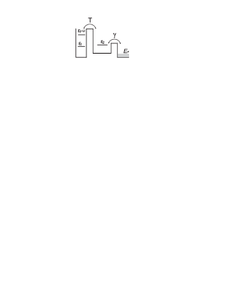
Figure 1: Scheme of the proposed model. The system of interacting QDs is coupled with the continuous spectrum states by means of the tunneling rate $\gamma=\pi\nu_{0}t^{2}$.

$$\hat{H}=\hat{H}_{D}+\hat{H}_{tun}+\hat{H}_{res}.$$ (1)

The Hamiltonian $\hat{H_{D}}$ of interacting QDs

$$\hat{H}_{D} = \sum_{i=1,2\sigma}\varepsilon_{i}c^{+}_{i\sigma}c_{i\sigma}+Un_{1\sigma}n_{1-\sigma}$$ (2)

$$+ \sum_{\sigma}T(c_{1\sigma}^{+}c_{2\sigma}+c_{1\sigma}c_{2\sigma}^{+}),$$

contains the spin-degenerate levels $\varepsilon_{i}$ (indexes $i=1$ and $i=2$ correspond to the first and to the second QD) and the on-site Coulomb repulsion for the double occupation of the first dot. For simplicity we consider Coulomb interaction only in the first QD though it is possible to obtain closed system of equations for filling numbers correlators in a general case taking into account Coulomb interaction between all the electrons localized in the dots. Our model is suitable for the case when the first QD is narrow and the second one is rather wide.Mantsevich_1 ; Kikoin_1 Besides, if electrons are initially located in the first QD and the second dot is empty, then filling numbers for the electrons in the second QD remain rather small during the time evolution of the charge and Coulomb effects in the second QD are not so important as in the first one.

The creation/annihilation of an electron with spin $\sigma=\pm 1$ within the dot is denoted by $c^{+}_{i\sigma}/c_{i\sigma}$ and $n_{\sigma}$ is the corresponding filling number operator. The coupling between the dots is described by the tunneling transfer amplitude $T$ which is considered to be independent of momentum and spin.

The continuous spectrum states are modeled by the Hamiltonian:

$$\hat{H}_{res}=\sum_{p\sigma}\varepsilon_{p}c^{+}_{p\sigma}c_{p\sigma},$$ (3)

where $c^{+}_{p\sigma}/c_{p\sigma}$ creates/annihilates an electron with spin $\sigma$ and momentum $p$ in the lead. The coupling between the second dot and the continuous spectrum states is described by the Hamiltonian:

$$\hat{H}_{tun}=\sum_{p\sigma}t(c_{p\sigma}^{+}c_{2\sigma}+c_{p\sigma}c_{2\sigma}^{+}),$$ (4)

where $t$ is the tunneling amplitude, which we assume to be independent on momentum and spin. By considering a constant density of states in the reservoir $\nu_{0}$, the tunnel rate $\gamma$ is defined as $\gamma=\pi\nu_{0}t^{2}$.

As we are interested in the specific features of the non-stationary time evolution of the initially localized charge in the coupled QDs, we’ll consider the situation when condition $(\varepsilon_{i}-\varepsilon_{F})/\gamma>>1$ is fulfilled. It means that initial energy levels are situated well above the Fermi level and stationary occupation numbers in the second QD in the absence of coupling between the QDs is of the order $\gamma/(\varepsilon_{2}-\varepsilon_{F})<<1$ and can be omitted. Consequently the Kondo effect is also negligible in the proposed model.

Our investigations deal with the low temperature regime when Fermi level is well defined and the temperature is much lower than all typical relaxation rates in the system. Consequently the distribution function of electrons in the leads (band electrons) is a Fermi step.

We set $\hbar=1$ and therefore the kinetic equations for bilinear combinations of Heisenberg operators $c_{i\sigma}^{+}/c_{i\sigma}$

$$c_{1\sigma}^{+}c_{1\sigma}=\hat{n}_{1}^{\sigma}(t);\quad c_{2\sigma}^{+}c_{2\sigma}=\hat{n}_{2}^{\sigma}(t);$$

$$c_{1\sigma}^{+}c_{2\sigma}=\hat{n}_{12}^{\sigma}(t);\quad c_{2\sigma}^{+}c_{1\sigma}=\hat{n}_{21}^{\sigma}(t),$$ (5)

which describe time evolution of the filling numbers for the electrons can be written as:

$$i\frac{\partial}{\partial t}\hat{n}_{1}^{\sigma} = -T(\hat{n}_{21}^{\sigma}-\hat{n}_{12}^{\sigma}),$$

$$i\frac{\partial}{\partial t}\hat{n}_{2}^{\sigma} = T(\hat{n}_{21}^{\sigma}-\hat{n}_{12}^{\sigma})-2i\gamma\hat{n}_{2}^{\sigma},$$

$$i\frac{\partial}{\partial t}\hat{n}_{21}^{\sigma} = T(\hat{n}_{2}^{\sigma}-\hat{n}_{1}^{\sigma})-(\xi+U\hat{n}_{1}^{-\sigma})\hat{n}_{21}^{\sigma}-i\gamma\hat{n}_{21}^{\sigma},$$

$$i\frac{\partial}{\partial t}\hat{n}_{12}^{\sigma} = -T(\hat{n}_{2}^{\sigma}-\hat{n}_{1}^{\sigma})+(\xi+U\hat{n}_{1}^{-\sigma})\hat{n}_{12}^{\sigma}-i\gamma\hat{n}_{12}^{\sigma},$$

where $\xi=\varepsilon_{1}-\varepsilon_{2}$ is the detuning between the energy levels in the QDs. The system of Eqs. (LABEL:system) contain expressions for the pair correlators $\hat{n}_{1}^{-\sigma}\hat{n}_{21}^{\sigma}$ and $\hat{n}_{1}^{-\sigma}\hat{n}_{12}^{\sigma}$, which also determine relaxation of the localized charge and consequently have to be evaluated. In this system we neglect high order correlation functions between localized and continuous spectrum (band) electrons and fulfill averaging over electron states in the reservoir.

Let us introduce the following designation for the pair correlators: $K_{iji^{{}^{\prime}}j^{{}^{\prime}}}^{\sigma\sigma^{{}^{\prime}}}=<c_{i\sigma}^{+}c_{j\sigma}c_{i^{{}^{\prime}}\sigma^{{}^{\prime}}}^{+}c_{j^{{}^{\prime}}\sigma^{{}^{\prime}}}>$ and consider only the paramagnetic case $<\hat{n}_{i}^{\sigma}>=<\hat{n}_{i}^{-\sigma}>$. Then the following relations take place

$$K_{2111}^{\sigma-\sigma} = <\hat{n}_{21}^{\sigma}\hat{n}_{1}^{-\sigma}>=<\hat{n}_{21}^{-\sigma}\hat{n}_{1}^{\sigma}>,$$

$$K_{1211}^{\sigma-\sigma} = <\hat{n}_{12}^{\sigma}\hat{n}_{1}^{-\sigma}>=<\hat{n}_{12}^{-\sigma}\hat{n}_{1}^{\sigma}>.$$ (7)

The system of equations for pair correlators can be written in the compact matrix form (symbol $[\quad]$ means commutation and symbol $\{\quad\}$- anticommutation):

$$i\frac{\partial}{\partial t}\widehat{K}=[\widehat{K},\widehat{H}^{{}^{\prime}}]+\{\widehat{K},\widehat{\Gamma}\}+\widehat{\Upsilon},$$ (8)

where $\widehat{K}$ is the pair correlators matrix

$$\widehat{K}=\begin{pmatrix}K_{2211}^{\sigma-\sigma}&K_{1211}^{\sigma-\sigma}&K_{2221}^{\sigma-\sigma}&K_{1221}^{\sigma-\sigma}\\ K_{2111}^{\sigma-\sigma}&K_{1111}^{\sigma-\sigma}&K_{2121}^{\sigma-\sigma}&K_{1121}^{\sigma-\sigma}\\ K_{2212}^{\sigma-\sigma}&K_{1212}^{\sigma-\sigma}&K_{2222}^{\sigma-\sigma}&K_{1222}^{\sigma-\sigma}\\ K_{2112}^{\sigma-\sigma}&K_{1112}^{\sigma-\sigma}&K_{2122}^{\sigma-\sigma}&K_{1122}^{\sigma-\sigma}\\ \end{pmatrix}=||K_{ij}||,$$ (9)

matrix $\widehat{H}^{{}^{\prime}}$ has the following form

$$\widehat{H}^{{}^{\prime}}=\begin{pmatrix}0&T&T&0\\ T&\xi+U&0&T\\ T&0&-\xi&T\\ 0&T&T&0\\ \end{pmatrix},$$ (10)

and the tunneling coupling matrix $\widehat{\Gamma}$ is denoted as:

$$\widehat{\Gamma}=\begin{pmatrix}-i\gamma&0&0&0\\ 0&0&0&0\\ 0&0&-2i\gamma&0\\ 0&0&0&-i\gamma\\ \end{pmatrix}.$$ (11)

One can easily find that Eqs. (8) contain expressions for the high-order correlators $K_{121122}^{\sigma-\sigma-\sigma}$ and $K_{211122}^{\sigma-\sigma-\sigma}$. Their contribution can be easily written in the matrix form $\widehat{\Upsilon}$:

$$\widehat{\Upsilon}=\begin{pmatrix}0&0&UK_{211122}^{\sigma-\sigma-\sigma}&0\\ 0&0&0&0\\ UK_{121122}^{\sigma-\sigma-\sigma}&0&0&UK_{211122}^{\sigma-\sigma-\sigma}\\ 0&0&UK_{121122}^{\sigma-\sigma-\sigma}&0\\ \end{pmatrix}.$$ (12)

Since the evolution starts from the initial state with two electrons in the first QD and empty second one, the system of Eqs. (8) for the pair correlators satisfies the initial conditions: $K_{1111}^{\sigma-\sigma}(0)=1$; $K_{2222}^{\sigma-\sigma}(0)=0$; $K_{iji^{{}^{\prime}}j^{{}^{\prime}}}^{\sigma-\sigma}(0)=0$ for the other combinations of indexes $i$, $j$. The high-order correlators $K_{121122}^{\sigma-\sigma-\sigma}$ and $K_{211122}^{\sigma-\sigma-\sigma}$ are exactly equal to zero due to the fact that they are the solution of the linear homogeneous system of equations with zero initial conditions.

The formal solution of the system for the pair correlators [see Eq. (8)] can be written with the help of the evolution operator. Time evolution of the matrix elements $K_{ij}$ [see Eq. (9)] is given by the expression:

$$K_{ij}(t)=\sum_{mn}(e^{-i\widehat{H}t})_{im}K_{mn}(0)(e^{i\widehat{H}^{+}t})_{nj},$$ (13)

where $\widehat{H}$ is defined as: $\widehat{H}=\widehat{H}^{{}^{\prime}}+\widehat{\Gamma}\\$.

Let us introduce the evolution operator:

$$\Phi_{ij}(t)=(e^{-i\widehat{H}t})_{ij}.$$ (14)

Consequently, the time evolution of the pair correlators can be found from the following expressions:

$$K_{2111}^{\sigma-\sigma} = (e^{-i\widehat{H}t})_{12}K(0)_{22}(e^{i\widehat{H}^{+}t})_{22}=\Phi_{12}(t)\widetilde{\Phi}_{22}(t),$$

$$K_{1211}^{\sigma-\sigma} = (e^{-i\widehat{H}t})_{22}K(0)_{22}(e^{i\widehat{H}^{+}t})_{21}=\Phi_{22}(t)\widetilde{\Phi}_{21}(t).$$

Since $K(0)_{22}$ in the matrix [see Eq. (9)] is equal to $K_{1111}^{\sigma-\sigma}(0)=1$. The evolution operator $\widetilde{\Phi}_{22}(t)$ can be obtained from the expression for the operator $\Phi_{22}(t)$ by the following substitutions: $t\rightarrow-t$ and $\gamma\rightarrow-\gamma$. Pair correlator $K_{1211}^{\sigma-\sigma}$ is a complex conjugate of $K_{2111}^{\sigma-\sigma}$.

Finally the evolution operators $\Phi_{ij}(t)$ are determined by the equations:

$$\begin{pmatrix}i\frac{\partial}{\partial t}\Phi_{12}(t)\\ i\frac{\partial}{\partial t}\Phi_{22}(t)\\ i\frac{\partial}{\partial t}\Phi_{32}(t)\\ i\frac{\partial}{\partial t}\Phi_{42}(t)\\ \end{pmatrix}=\widehat{H}\cdot\begin{pmatrix}\Phi_{12}(t)\\ \Phi_{22}(t)\\ \Phi_{32}(t)\\ \Phi_{42}(t)\\ \end{pmatrix},$$ (16)

with the initial conditions:

$$\Phi_{ij}(0)=\delta_{ij}.$$ (17)

The characteristic equation for the evolution operator $\Phi_{ij}(t)$ eigenvalues $\lambda_{i}$ has the form:

$$(H_{11}-\lambda)(H_{22}-\lambda)(H_{33}-\lambda)(H_{44}-\lambda)-T^{2}$$

$$\times[(H_{11}-\lambda)(H_{22}-\lambda)+(H_{11}-\lambda)(H_{33}-\lambda)$$

$$+(H_{33}-\lambda)(H_{44}-\lambda)+(H_{22}-\lambda)(H_{44}-\lambda)]=0,$$

where coefficients $H_{11}$, $H_{22}$, $H_{33}$ and $H_{44}$ are determined as:

$$H_{11} = H_{44}=-i\gamma,$$

$$H_{22} = \xi+U,$$

$$H_{33} = -\xi-2i\gamma.$$ (19)

Each eigenvalue $\lambda_{i}$ determines the corresponding eigenvector:

$$\psi_{i}=\begin{pmatrix}\alpha_{i}\\ \beta_{i}\\ \gamma_{i}\\ \delta_{i}\\ \end{pmatrix}.$$ (20)

In our case it is necessary to obtain expressions for the evolution operators $\Phi_{12}(t)$ and $\Phi_{22}(t)$ with the initial conditions $\Phi_{22}(0)=1$ and $\Phi_{ij}(0)=0$.

Solution for the system of equations which determines the functions $\Phi_{12}(t)$ and $\Phi_{22}(t)$ can be written as:

$$\Phi_{12}(t)=\sum_{i=1}^{4}C_{i}\alpha_{i}e^{-i\lambda_{i}t},$$

$$\Phi_{22}(t)=\sum_{i=1}^{4}C_{i}\beta_{i}e^{-i\lambda_{i}t}.\$$ (21)

where, constants $C_{i}$ can be obtained from the initial conditions for the system of equations.

$$\sum_{i}C_{i}\alpha_{i}=0,$$

$$\sum_{i}C_{i}\beta_{i}=1,$$

$$\sum_{i}C_{i}\gamma_{i}=0,$$

$$\sum_{i}C_{i}\delta_{i}=0.\$$ (22)

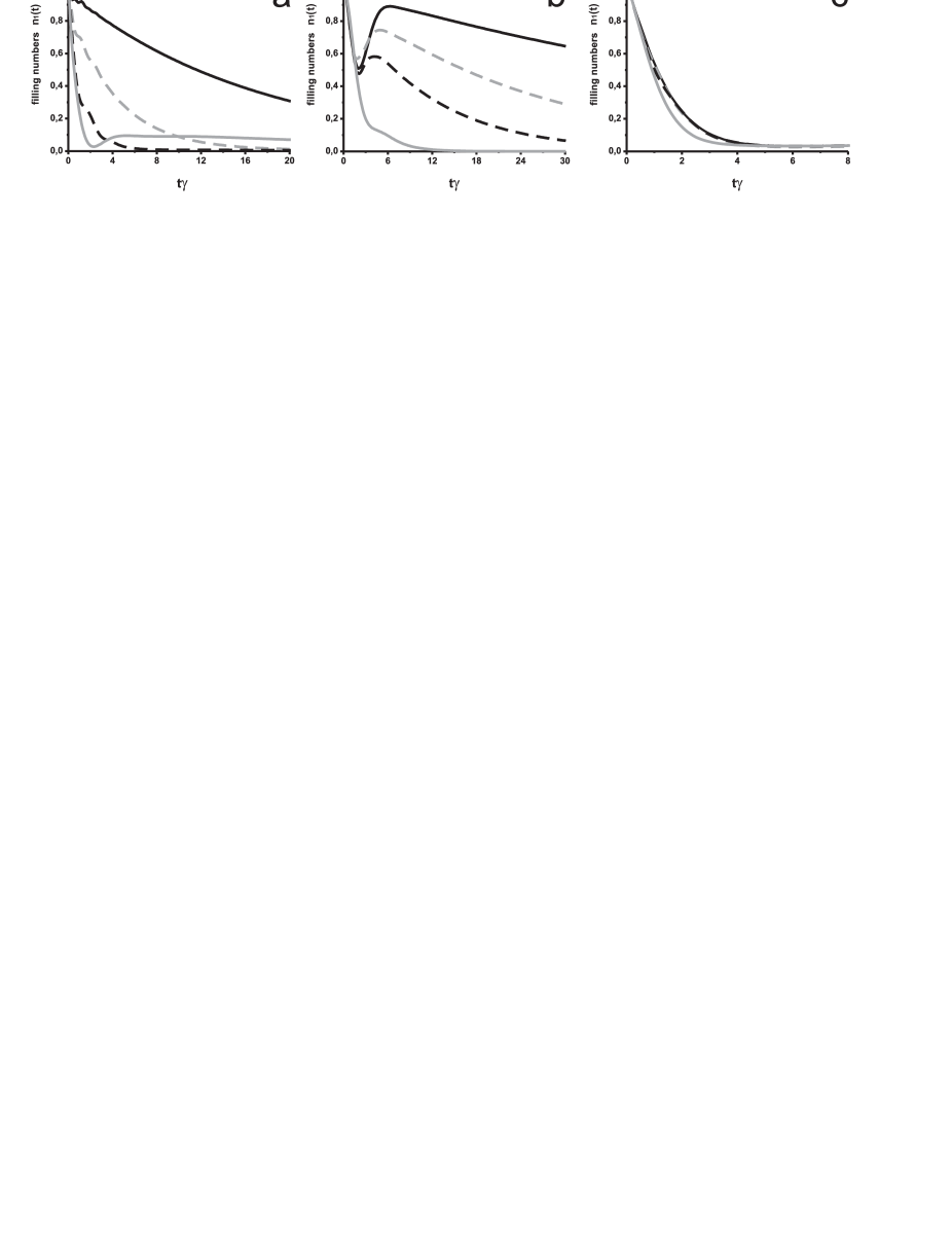
Figure 2: Different time evolution regimes of the filling numbers $n_{1}(t)$ in the first QD in the presence of Coulomb interaction. a). $(\xi+U)/\gamma=0$ ($U/\gamma=10$, $\xi/\gamma=-10$- black line; $U/\gamma=5$, $\xi/\gamma=-5$- grey dashed line; $U/\gamma=3$, $\xi/\gamma=-3$- black dashed line; $U/\gamma=1$, $\xi/\gamma=-1$- grey line); b). $\frac{\xi+U}{\gamma}\sim 1$ ($U/\gamma=10$, $\xi/\gamma=-7$- black line; $U/\gamma=5$, $\xi/\gamma=-4$- grey dashed line; $U/\gamma=3$, $\xi/\gamma=-2.5$- black dashed line; $U/\gamma=1$, $\xi/\gamma=-0.75$- grey line); c). $\xi/\gamma=0$ ($U/\gamma=10$- black line; $U/\gamma=5$- grey dashed line; $U/\gamma=3$- black dashed line; $U/\gamma=1$- grey line). Parameters $T/\gamma=0.6$, $\gamma=1$ are the same for all the figures.

II.1 Equations for the time dependent filling numbers

The time dependent filling numbers $n_{1}(t)$ can be found from the inhomogeneous part of Eqs. (LABEL:system), which results in:

$$\{[(i\frac{\partial}{\partial t}+i\gamma)^{2}+\gamma^{2}][(i\frac{\partial}{\partial t}+i\gamma)^{2}-\xi^{2}]$$

$$-4T^{2}(i\frac{\partial}{\partial t}+i\gamma)^{2}\}n_{1}(t)=(i\frac{\partial}{\partial t}+2i\gamma)$$

$$\times TU(G_{2}^{-1}K_{2111}^{\sigma-\sigma}+G_{1}^{-1}K_{1211}^{\sigma-\sigma}),$$ (23)

where operators $G_{2}^{-1}$ and $G_{1}^{-1}$ have the form:

$$G_{2}^{-1} = i\frac{\partial}{\partial t}+\xi+i\gamma,$$

$$G_{1}^{-1} = i\frac{\partial}{\partial t}-\xi+i\gamma.$$ (24)

Solution of the Eq. (23) describes localized charge relaxation and consists of the two parts: the first one is the general solution of the homogeneous equation $n_{1}^{h}(t)$ (right hand part is equal to zero) and the second one is the partial solution of the inhomogeneous equation $\widetilde{n}_{1}(t)$.

$$n_{1}(t) = n_{1}^{h}(t)+\widetilde{n}_{1}(t)$$ (25)

$$= n_{1}^{h}(t)+\int_{0}^{t}\textit{{G}}(t-t^{{}^{\prime}})P(t^{{}^{\prime}})dt^{{}^{\prime}},$$

where $\textit{{G}}(t-t^{{}^{\prime}})$- is the Green function of the Eq. (23) with $\delta(t-t^{{}^{\prime}})$ in the right hand part, and $P(t^{{}^{\prime}})$-is the right hand part of the Eq. (23), which appears due to the Coulomb correlations.

General solution of the homogeneous equation has the form: Pump

$$n_{1}^{h}(t) = n_{1}^{0}[A^{{}^{\prime}}e^{-i(E_{1}-E_{1}^{*})t}$$ (26)

$$+ 2Re(B^{{}^{\prime}}e^{-i(E_{1}-E_{2}^{*})t})+C^{{}^{\prime}}e^{-i(E_{2}-E_{2}^{*})t}],$$

where coefficients $A^{\prime}$, $B^{\prime}$ and $C^{\prime}$ are determined as:

$$A^{{}^{\prime}} = \frac{|E_{2}-\varepsilon_{1}|^{2}}{|E_{2}-E_{1}|^{2}};\quad C^{{}^{\prime}}=\frac{|E_{1}-\varepsilon_{1}|^{2}}{|E_{2}-E_{1}|^{2}};$$

$$B^{{}^{\prime}} = -\frac{(E_{2}-\varepsilon_{1})(E_{1}^{*}-\varepsilon_{1})}{|E_{2}-E_{1}|^{2}}.$$ (27)

Eigenfrequencies $E_{i}$ can be found from the equation:

$$(E-\varepsilon_{1})(E-\varepsilon_{2}+i\gamma)-T^{2}=0,$$ (28)

and have the form

$$E_{1,2}=\frac{1}{2}(\varepsilon_{1}+\varepsilon_{2}-i\gamma)$$

$$\pm\frac{1}{2}\sqrt{(\varepsilon_{1}-\varepsilon_{2}+i\gamma)^{2}+4T^{2}}.$$ (29)

Green function $\textit{{G}}(t-t^{{}^{\prime}})$ of the Eq. (23) can be written as:

$$\textit{{G}}(t-t^{{}^{\prime}})=\sum_{i=1}^{4}a_{i}e^{-i\lambda_{i}(t-t^{{}^{\prime}})}\Theta(t-t^{{}^{\prime}}),$$ (30)

where $\lambda_{i}$-are the roots of the characteristic equation arising from Eq. (23) :

$$\lambda_{1,2} = -i\gamma\pm[\frac{4T^{2}+\xi^{2}-\gamma^{2}}{2}$$

$$+ \frac{1}{2}\sqrt{(4T^{2}+\xi^{2}-\gamma^{2})^{2}+4\xi^{2}\gamma^{2}}]^{1/2},$$

$$\lambda_{3,4} = -i\gamma\pm[\frac{4T^{2}+\xi^{2}-\gamma^{2}}{2}$$ (31)

$$- \frac{1}{2}\sqrt{(4T^{2}+\xi^{2}-\gamma^{2})^{2}+4\xi^{2}\gamma^{2}}]^{1/2},$$

these roots are connected with the eigenfrequencies $E_{i}$ by the relations

$$\lambda_{1,2} = E_{1,2}-E_{1,2}^{*},$$

$$\lambda_{3} = E_{1}-E_{2}^{*},$$

$$\lambda_{4} = E_{2}-E_{1}^{*}.$$ (32)

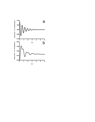
Figure 3: Oscillating terms for the two different time evolution regimes of the filling numbers $n_{1}(t)$. a). $\xi/\gamma=0$; b). $(\xi+U)/\gamma=0$. Parameters $T/\gamma=0.6$, $\gamma=1$, $U/\gamma=10$ are the same for all the figures.

Coefficients $a_{i}$ are determined as:

$$a_{1}=\frac{1}{(\lambda_{2}-\lambda_{1})(\lambda_{3}-\lambda_{1})(\lambda_{4}-\lambda_{1})},$$

$$a_{2}=\frac{1}{(\lambda_{1}-\lambda_{2})(\lambda_{3}-\lambda_{2})(\lambda_{4}-\lambda_{2})},$$

$$a_{3}=\frac{1}{(\lambda_{1}-\lambda_{3})(\lambda_{2}-\lambda_{3})(\lambda_{4}-\lambda_{3})},$$

$$a_{4}=\frac{1}{(\lambda_{1}-\lambda_{4})(\lambda_{2}-\lambda_{4})(\lambda_{3}-\lambda_{4})}.$$ (33)

Let us now focus on the two limit cases when the expressions which determine the dynamics of the filling numbers have a rather compact form. The first one corresponds to the situation when the detuning between the empty energy levels in the QDs is equal to zero: $\xi/\gamma\ll 1$. The second one deals with the situation when the sum of the detuning and the half value of Coulomb interaction is equal to zero. This means that the resonance between the half occupied energy level in the first QD and the empty level in the second QD takes place: $(\xi+U)/\gamma\ll 1$. We shall also consider that in both cases the condition $T\ll\gamma\ll U$ is fulfilled.

II.2 $\xi/\gamma\ll 1$

The eigenvalues of the characteristic equation in the first case ($\xi/\gamma\ll 1$) within the accuracy $\frac{T^{2}}{U^{2}}$ have the form:

$$\lambda_{1} = U-i\frac{2T^{2}\gamma}{U^{2}},$$

$$\lambda_{2} = -i\gamma-i\frac{2T^{2}}{\gamma},$$

$$\lambda_{3} = -2i\gamma-i\frac{2T^{2}}{\gamma},$$

$$\lambda_{4} = -i\gamma.$$ (34)

So, the evolution operators can be written as:

$$\Phi_{12}(t) = \frac{T}{U}(e^{-iUt-\frac{2T^{2}\gamma}{U^{2}}t}-e^{-\gamma t-\frac{2T^{2}}{\gamma}t}),$$

$$\Phi_{22}(t) = (1-\frac{2T^{2}}{U^{2}})e^{-iUt-\frac{2T^{2}\gamma}{U^{2}}t}+\frac{2T^{2}}{U^{2}}e^{-\gamma t-\frac{2T^{2}}{\gamma}t},$$

and time dependence of the pair correlators $K_{2111}^{\sigma-\sigma}$ and $K_{1211}^{\sigma-\sigma}$ is determined by the product:

$$K_{2111}^{\sigma-\sigma}(t) = \Phi_{12}(t)\Phi_{22}^{*}(t),$$

$$K_{1211}^{\sigma-\sigma}(t) = (K_{2111}^{\sigma-\sigma})^{*}.$$ (36)

Expression for the $P(t)$ [see Eq. (25)] in the case of the resonance between empty levels $\xi/\gamma=0$ has the form:

$$P(t)=4T^{2}\gamma e^{-\frac{4T^{2}\eta}{\gamma}t}+2T^{2}Ue^{-\gamma t}\cos(Ut),$$ (37)

where $\eta=\frac{\gamma^{2}}{U^{2}+\gamma^{2}}$. For $\eta=1/2$ the inhomogeneous part of the time evolution of the filling numbers $\widetilde{n}_{1}(t)$ can be written as:

$$\widetilde{n}_{1}(t) = \frac{T^{2}}{\gamma^{2}}[(-2\gamma t-e^{-\frac{2T^{2}}{\gamma}t})e^{-\frac{2T^{2}}{\gamma}t}+e^{-2\gamma t}$$ (38)

$$+ 4e^{-\frac{2T^{2}}{\gamma}t}-4e^{-\gamma t}]+\frac{2T^{2}Ue^{-\gamma t}}{\gamma^{3}}[cos(Ut)-1]$$

$$+ 0(\frac{T^{2}}{U^{2}}\frac{\gamma}{U}).$$

For $\eta\ll 1$ the time evolution of the filling numbers $\widetilde{n}_{1}(t)$ can be determined by:

$$\widetilde{n}_{1}(t)=\frac{1}{1-2\eta}(e^{-4\frac{T^{2}\eta}{\gamma}t}-e^{-\frac{2T^{2}}{\gamma}t})+0(\frac{T^{2}}{\gamma^{2}}).$$ (39)

II.3 $(\xi+U)/\gamma\ll 1$

In the second case of interest ($(\xi+U)/\gamma\ll 1$ but $U/\gamma\gg 1$) eigenvalues are:

$$\lambda_{1} = \frac{U}{2}-i\frac{8T^{2}\gamma}{U^{2}},$$

$$\lambda_{2} = -i\gamma+\frac{8T^{2}}{U},$$

$$\lambda_{3} = -2i\gamma+\frac{U}{2}-\frac{i8T^{2}\gamma}{U^{2}}+\frac{4T^{2}}{U},$$

$$\lambda_{4} = -i\gamma.$$ (40)

Evolution operators have the following form:

$$\Phi_{12}(t) = \frac{2T}{U}(e^{-i\frac{U}{2}t-\frac{8T^{2}\gamma}{U^{2}}t}-e^{-\gamma t}),$$

$$\Phi_{22}(t) = (1-\frac{8T^{2}}{U^{2}})e^{-i\frac{U}{2}t-\frac{8T^{2}\gamma}{U^{2}}t}+\frac{8T^{2}}{U^{2}}e^{-\gamma t}.$$ (41)

When the condition $(\xi+U)/\gamma=0$ is fulfilled, $P(t)$ within the accuracy $\frac{T^{3}}{U^{3}}$ and $\frac{\gamma^{2}}{U^{2}}$ is determined by the expression:

$$P(t)=-T^{2}U^{2}(e^{i\frac{U}{2}t-\gamma t}+h.c.)-4T^{2}\gamma^{2}e^{-\frac{16T^{2}\gamma}{U^{2}}t}.$$

The inhomogeneous part of the time evolution of the filling numbers $\widetilde{n}_{1}(t)$ with the accuracy $\frac{T^{2}}{U^{2}}$ has the form:

$$\widetilde{n}_{1}(t) = -\frac{4}{7}(1-e^{-14\frac{T^{2}\gamma}{U^{2}}t})e^{-\frac{2T^{2}\gamma}{U^{2}}t}$$ (43)

$$- 2\frac{T^{2}}{\gamma U}e^{-\gamma t}\sin(\frac{U}{2}t)+0(\frac{T^{2}}{U^{2}}).$$

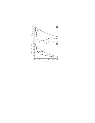
Figure 4: Time dependence of the filling numbers for the electrons $n_{1}(t)$ in the presence of Coulomb interaction: comparison of the exact solution and the mean-field approximation. Black line corresponds to the exact solution, black dashed line corresponds to the mean-field approximation. Grey line demonstrates relaxation of the localized charge in the absence of Coulomb interaction. a). $U/\gamma=5$, $\xi/\gamma=-3$; b). $U/\gamma=3$, $\xi/\gamma=-2$. Parameters $T/\gamma=0.6$, $\gamma=1$ are the same for all the figures.

It is necessary to point out that relaxation of the filling numbers in the proposed model can be analyzed by means of more simple method — the self-consistent mean-field approximation.Anderson ; Mantsevich_1 In this approximation correlation functions $U\langle\hat{n}_{i}^{-\sigma}\hat{n}_{ij}^{\sigma}\rangle$ in the Eqs. (LABEL:system) are substituted by the expressions $U\langle\hat{n}_{i}^{-\sigma}\rangle\langle\hat{n}_{ij}^{\sigma}\rangle$. Such substitution is valid in the case when filling numbers for the localized electrons $n_{i}^{-\sigma}$ change their values rather slow. Calculation scheme consists of the two steps. On the first step one has to substitute the initial energy level position $\varepsilon_{i}$ by the expression $\widetilde{\varepsilon}_{i}=\varepsilon_{i}+U\langle\hat{n}_{i}^{-\sigma}\rangle$ and to evaluate the time dependent filling numbers. The second step deals with the self-consistent calculation of the time dependent filling numbers for the electrons. For some ranges of the system parameters mean-field approximation reveals qualitatively good results. Mantsevich_1 But in general case the mean-field approximation is insufficient to describe the relaxation processes in the system with correlations.

III Results and discussion

Time evolution of the filling numbers for the electrons strongly depends on the relations between the system parameters.

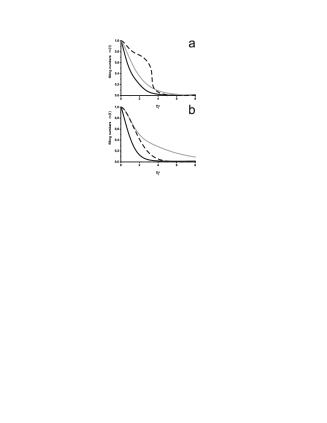
Figure 5: Relaxation of the filling numbers $n_{1}(t)$ in the presence of Coulomb interaction in the case of the resonant tunneling between the empty energy levels in the QDs. Black line corresponds to the exact solution, black dashed line corresponds to the mean-field approximation. Grey line demonstrates relaxation of the localized charge in the absence of Coulomb interaction. a). $\xi/\gamma=0$, $U/\gamma=3$; b). $\xi/\gamma=0$, $U/\gamma=1$. Parameters $T/\gamma=0.6$, $\gamma=1$ are the same for all the figures.

If condition $(\xi+U)/\gamma\ll 1$ is fulfilled, the Coulomb interaction value increasing leads to the decreasing of the filling numbers relaxation rate [see Fig. 2(a)]. For the large $U$ relaxation rate is rather slow and is of the order of $\gamma_{nonres}=2\frac{T^{2}\gamma}{U^{2}}$ which is typical for the system of two coupled QDs without Coulomb interaction with $|\xi|\simeq U$. By the decreasing of the Coulomb interaction value $U$ we achieve the situation of resonant tunneling between the localized states and consequently relaxation rate becomes larger. On the Fig. 2(c) the situation of resonant tunneling between the empty energy levels $\xi/\gamma=0$ is demonstrated. In this case the relaxation of the localized charge takes place with the typical rate very close to the value $\gamma_{res}=2\frac{T^{2}}{\gamma}$ and is almost independent on the Coulomb interaction value. Let us notice that relaxation processes are governed not only by the typical exponents $e^{-\gamma t}$ and $e^{-\frac{2T^{2}}{\gamma}t}$ but also by the pre-exponential factor, which linearly increases in time in the resonant case [see Eq. (38)].

A very special relaxation regime exists in the system if condition $\frac{\xi+U}{\gamma}\sim 1$ takes place [see Fig. 2(b)]. In this regime Coulomb correlations result in formation of a dip in the time evolution of the localized charge. At the initial relaxation stage the charge in the first QD rapidly decreases due to the almost resonant relation between the level in the second QD and effective single electron energy in the first dot. It follows from the third and the fourth Eqs. (LABEL:system) of the system that changing of the effective energy levels detuning is determined by $URe[\frac{\langle\hat{n}_{1}^{-\sigma}(t)\hat{n}_{12}^{\sigma}(t)\rangle}{\langle\hat{n}_{12}^{\sigma}(t)\rangle}]$ which differs from the typical mean-field expression $U\langle\hat{n}_{i}^{-\sigma}(t)\rangle$. Anderson

At a certain instant of time the effective single electron level falls down beneath the level in the second QD. At this moment the inverse charge begins to flow from the second QD to the first one. The occupation in the first QD demonstrates significant increasing after reaching minima value (the dip formation). Filling numbers almost reach the initial value for the large values of Coulomb interaction. After the dip formation the typical time scale which determines relaxation of the filling numbers is close enough to the value $\gamma_{nonres}=2\frac{T^{2}\gamma}{\xi^{2}}$. This explanation gives qualitative picture of the dips formation. The exact solution shows, that Coulomb correlations are responsible for such non-monotonic behavior. This effect is determined by the inhomogeneous part of the exact solution for time evolution of the filling numbers in the first QD [see the first term in Eq. (43)]. And this inhomogeneous part appears due to complete account for time dependence of the high order correlators [$P(t)$ in Eq (23) and Eq. (25))]. That is why time evolution of the filling numbers for the electrons differs considerably from mean-field approximation. The width of the dip can be roughly estimated as $1/8\cdot\gamma_{nonres}^{-1}$.

We would like to stress that the non-monotonic behavior, which we discussed above, is not connected with the usual quantum oscillations between two energy levels. Such oscillations also take place during time evolution, but the amplitude of these oscillations is rather small (of the order $\frac{T^{2}}{U^{2}}$). Only these small oscillating contributions to the total electron density are shown on the Fig. 3. Oscillations are always present in the case of strong Coulomb interaction for all the values of the ratio $T/\gamma$. We found out that besides the oscillations governed by the system parameters $T$ and $U$, oscillations with the double period exist in the system. Oscillation period doubling is mostly pronounced in the case when resonant tunneling takes place between the half occupied energy level in the first QD with the initial charge and empty level in the dot coupled with the continuous spectrum states $(\xi+U)/\gamma\ll 1$ [see Fig. 3(b)]. Double period oscillations disappears with the decreasing of energy levels detuning $\xi$. In this case oscillations period is determined by the value of the Coulomb interaction [see Eq. (38)].

Comparison between the exact solution and the mean-field approximation is demonstrated on the Figs. 4-5. It is clearly evident that both methods reveal such similar peculiarities of the system behavior as several time ranges with considerably different relaxation rates. For some ranges of the system parameters formation of the dip can be also reproduced in the mean-field approximation (see Fig. 4). Figure 4 also demonstrates similar behavior of the exact and the mean-field solutions at the initial stage of relaxation. But the dip reproduces incorrectly in the mean-field approximation.

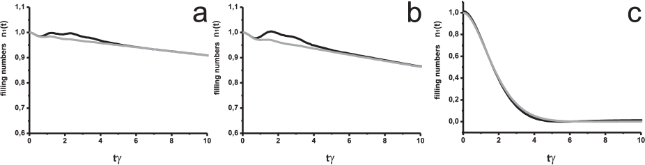
Figure 6: The influence of the Coulomb interaction in the second QD on the time evolution of the filling numbers $n_{1}(t)$ in the first QD. Black line corresponds to the exact solution. Grey line demonstrates relaxation of the localized charge in the absence of Coulomb interaction. a).$\xi/\gamma=-5$; b).$\xi/\gamma=-4$; c).$\xi/\gamma=0$. Parameters $T/\gamma=0.6$, $\gamma=1$, $U/\gamma=5$ are the same for all the figures.

In the case of resonant tunneling between the energy levels in the QDs ($\xi/\gamma=0$) the exact solution and the mean-field approximation reveal strong mismatch [see Fig. 5(a)]. Exact solution demonstrates rather smooth time evolution of the localized charge while the solution obtained by means of the mean-field approximation reveals abrupt changing of the localized charge amplitude. If the Coulomb repulsion decreases the correspondence between the exact and the mean-field solutions becomes better [see Fig. 5(b)]

Finally let us return to the influence of the Coulomb repulsion in the second QD on the evolution of the filling numbers. In this situation time evolution of the filling numbers for the electrons can be analyzed by means of the equations obtained for the model when Coulomb interaction acts in the first QD [see Eq. (LABEL:system)] after substituting the value $U\hat{n}_{1}^{-\sigma}$ by the $U\hat{n}_{2}^{-\sigma}$ in the Eq. (LABEL:system). The results are shown on the Fig. 6 and it is clearly evident that in this case the influence of Coulomb correlations on the relaxation of the filling numbers is rather weak.

IV Conclusions

We have studied time evolution of the filling numbers in the system of two interacting QDs coupled with the continuous spectrum states in the presence of Coulomb interaction in one of the dots for a wide range of the system parameters. The solution describing the system dynamics was analyzed in the assumption that the band and localized filling numbers for the electrons are uncoupled. This solution exactly takes into account all order correlators for the localized electrons in the QDs.

We found strongly different relaxation regimes in the system of coupled QDs depending on the ratios between the system parameters. Interesting manifestation of Coulomb correlations is the formation of the dip in the time evolution of the localized charge. Such reentrant charge behavior is not the result of simple quantum oscillations between the two energy levels. Oscillations of this type are also present in the system but have small amplitude in the case of the strong Coulomb interaction. Interaction effects lead to the appearance of oscillations with double period at particular range of parameters together with the oscillations governed by the detuning between the energy levels.

We compared our results with the mean-field approximation. The mean-field approximation can give in some cases qualitatively similar peculiarities of the system behavior: several time ranges with considerably different relaxation rates and dip’s formation. But in many regimes the results of the mean-field approximation do not coincide with the exact solution. Even if the mean-field approximation qualitatively correctly predicts appearance of the dip, it’s shape and width strongly differs from the exact solution.

V ACKNOWLEDGMENTS

This work was partly supported by the RFBR, Leading Scientific School grants and Russian Ministry of Science and Education programs.

References

• (1) C.P. Collier, E.W. Wong, M. Belohradsky, F.M. Raymo, J.F. Stoddart, P.J. Kuekes, R.S. Williams, and J.R. Heath, Science, 285, 391 (1999).
• (2) D.I. Gittins, D. Bethell, D.J. Schiffrin, and R.J. Nichols, Nature, 408, 67 (2000).
• (3) M.A. Kastner, Rev. Mod. Phys., 4, 849 (1992).
• (4) R. Ashoori, Nature, 379, 413 (1996).
• (5) T.H. Oosterkamp, T. Fujisawa, W.G. van der Wiel, K. Ishibashi, R.V. Hijman, S. Tarucha, and L. P. Kouwenhoven, Nature, 395, 873 (1998).
• (6) R.H. Blick, D. van der Weide, R.J. Haug, and K. Eberl, Phys.Rev Lett., 81, 689 (1998).
• (7) C.A. Stafford, and N. Wingreen, Phys. Rev. Lett., 76, 1916 (1996).
• (8) B.L. Hazelzet, M.R. Wagewijs, T.H. Stoof, and Yu.V. Nazarov, Phys.Rev. B, 63, 165313 (2001).
• (9) E. Cota, R. Aguadado, and G. Platero, Phys.Rev Lett., 94, 107202 (2005).
• (10) F.R. Waugh, M.J. Berry, D.J. Mar, R.M. Westervelt, K.L. Campman, and A.C. Gossard, Phys. Rev. Lett., 75, 705 (1995).
• (11) R.H. Blick, R.J. Haug, J. Weis, D. Pfannkuche, K.v. Klitzing, and K. Eberl, Phys.Rev B, 53, 7899 (1996).
• (12) C.A. Stafford, and S. Das Sarma, Phys. Rev. Lett., 72, 3590 (1994).
• (13) K.A. Matveev, L.I. Glazman, and H.U. Baranger, Phys.Rev. B, 54, 5637 (1996).
• (14) A.N. Vamivakas, C.-Y. Lu, C. Matthiesen, Y. Zhao, S. Fält, A. Badolato, and M. Atatüre, Nature Letters, 467, 297 (2010).
• (15) E.A. Stinaff, M. Scheibner, A.S. Bracker, I.V. Ponomarev, V.L. Korenev, M.E. Ware, M.F. Doty, T.L. Reinecke, and D. Gammon, Science, 311, 636 (2006).
• (16) J.M. Elzerman, K.M. Weiss, J. Miguel-Sanchez, and A. Imimoǧlu Phys. Rev. Lett., 107, 017401 (2011).
• (17) K. Kikoin, and Y. Avishai, Phys. Rev. B, 65, 115329 (2002).
• (18) J. Peng, and G. Bester, Phys. Rev. B, 82, 235314 (2010).
• (19) G. Munoz-Matutano, M. Royo, J.I. Climente, J. Canet-Ferrer, D. Fuster, P. Alonso-González, I. Fernández-Martínez, J. Martínez-Pastor, Y. González, L. González, F. Briones, and B. Alén , Phys. Rev. B, 84, 041308(R) (2011).
• (20) S. J. Angus, A.J. Ferguson, A.S. Dzurak, and R.G. Clark, Nano Lett., 7, 2051 (2007).
• (21) K. Grove-Rasmussen, H. Jorgensen, T. Hayashi, P.E. Lindelof, and T. Fujisawa, Nano Lett., 8, 1055 (2008).
• (22) S. Moriyama, D. Tsuya, E. Watanabe, S. Uji, M. Shimizu, T. Mori, T. Yamaguchi, and K. Ishibashi, Nano Lett., 9, 2891 (2009).
• (23) R. Landauer, Science, 272, 1914 (1996).
• (24) D. Loss, and D.P. DiVincenzo, Phys. Rev. A, 57, 120 (1998).
• (25) S.E. Nigg, and M. Buttiker, Phys. Rev. Lett., 102, 236801 (2009).
• (26) M. Filippone, K. Le Hur, and C. Mora, Phys. Rev. Lett., 107, 176601 (2011).
• (27) K.Y. Tan, K.W. Chan, M. Möttönen, A. Morello, C. Yang, J. van Donkelaar, A. Alves, J.-M. Pirkkalainen, D.N. Jamieson, R.G. Clark, and A.S. Dzurak, Nano Lett., 10, 11 (2010).
• (28) L.C.L. Hollenberg, A.D. Greentree, A.G. Fowler, and C. J. Wellard, Phys.Rev. B, 74, 045311 (2006).
• (29) G. Feve, A. Mahé, J.-M. Berroir, T. Kontos, B. Pla ais, D.C. Glattli, A. Cavanna, B. Etienne, and Y. Jin, Science, 316, 1169 (2007).
• (30) M. Lee, R. L pez, M.-S. Choi, T. Jonckheere, and T. Martin, Phys. Rev. B, 83, 201304(R) (2011).
• (31) F. Reckermann, J. Splettstoesser, and M.R. Wegewijs, Phys. Rev. Lett., 104, 226803 (2010).
• (32) T. Hayashi, T. Fujisawa, H. Cheong, Y.H. Jeong, and Y. Hirayama, Phys.Rev. Lett., 91, 226804 (2003).
• (33) L.D. Contreras-Pulido, J. Splettstoesser, M. Governale, J. König, and M. Büttiker, Phys. Rev. B, 85, 075301 (2012).
• (34) P. I. Arseyev, N. S. Maslova , and V. N. Mantsevich, JETP Letters, 95(10), 521 (2012).
• (35) P.I. Arseyev, N.S. Maslova, and V. N. Mantsevich, European Physical Journal B, 85(7), 249 (2012).
• (36) V.N. Mantsevich, N.S. Maslova, and P.I. Arseyev, Solid State Comm., 152, 1545 (2012).
• (37) K. Kikoin, and Y. Avishai, Phys.Rev. Lett., 86, 2090 (2001).
• (38) P.W. Anderson, Phys.Rev., 124, 41 (1961).