Husimi Maps in Graphene

Abstract

We present a method for bridging the gap between the Dirac effective field theory and atomistic simulations in graphene based on the Husimi projection, allowing us to depict phenomena in graphene at arbitrary scales. This technique takes the atomistic wavefunction as an input, and produces semiclassical pictures of quasiparticles in the two Dirac valleys. We use the Husimi technique to produce maps of the scattering behavior of boundaries, giving insight into the properties of wavefunctions at energies both close to and far from the Dirac point. Boundary conditions play a significant role to the rise of Fano resonances, which we examine using the Husimi map to deepen our understanding of bond currents near resonance.

I Introduction

With interest and experimental capabilities in graphene devices growing(Geim-Nature, ; Experiment1, ; Experiment2, ; Experiment3, ; Experiment5, ; Experiment4, ; Mario, ; Mario2-not-Mario, ), the need has never been greater to improve our understanding of quantum states in this material. Despite the success of the Dirac effective field theory for graphene(castro-neto, ), however, many technological proposals arise from predictions using the more fundamental tight-binding approximation(Wimmer-Spin-Currents-Rough-Nanoribbons, ; KaxirasNanoFlakes, ; Wimmer-Spin-Transport, ; WeiLi, ). This is because the atomistic model that underlies the Dirac theory is able to incorporate phenomena such as scattering from small defects(molecular-doping-graphene, ; imaging-edge-states, ; defect-graphene, ; defect-point-standing-wave, ; defects-graphene-point-theory-predict, ), ripples(katsnelson-ripples, ), or edge types(reconstructing-edges, ; imaging-edges, ; edge-types-effects, ) – all of which promise technological applications. However, atomistic calculations are computationally expensive, and replacing these features with scattering theories in a more-efficient Dirac model introduces substantial challenges. A robust approach which can analyze the atomistic wavefunction to produce semiclassical pictures of quasiparticles in the two Dirac valleys remains to be seen.

To address these issues and expand our understanding of graphene quantum states, we use the Husimi projection technique, introduced by Mason et al. (Mason-PRL, ; Mason-Husimi-Continuous, ; Mason-Husimi-Lattices, ), to produce snapshots of the local momentum distribution and underlying semiclassical structure in graphene wavefunctions. When Husimi projections are calculated at many points across a system, the Husimi map that results provides a semiclassical picture of the atomistic wavefunction. In this article, we define the Husimi map for graphene systems (Sec. II), and use it to deepen our understanding of boundary conditions in both high-energy relativistic scar states(PhysRevLett.53.1515, ; Huang-PRL-Scars, ) (Sec. III.1), and states near the Dirac point (Sec. III.2). We then use Husimi maps to interpret Fano resonances(fano-original, ; JJAP.36.3944, ; fano-review, ) within this novel material (Sec. III.3).

II Method

II.1 Definition of the Husimi Projection

The conduction band of the graphene system can be approximated as a honeycomb lattice with a single $p_{z}$ orbital located at each carbon-atom lattice site(castro-neto, ). The Husimi function is defined as a measurement between a wavefunction $\psi(\left\{\mathbf{r}_{i}\right\})$ defined at each orbital, and a coherent state $\left|\mathbf{r}_{0},\mathbf{k}_{0},\sigma\right\rangle$ which describes an envelope function over those sites that minimizes the joint uncertainty in spatial and momentum coordinates. The parameter $\sigma$ defines the spatial spread of the coherent state and defines the uncertainties in space and momentum according to the well-known relation

$$\Delta x\propto\frac{1}{\Delta k}\propto\sigma.$$ (1)

As a result, there is a trade-off for any value of $\sigma$ selected: for small $\sigma$, there is better spatial resolution but poorer resolution in $k$-space, and vice versa for large $\sigma$.

Writing out the dot product of the wavefunction and the coherent state

$$\left\langle\left.\psi\vphantom{\mathbf{r}_{0},\mathbf{k}_{0},\sigma}\right|\mathbf{r}_{0},\mathbf{k}_{0},\sigma\right\rangle = \left(\frac{1}{\sigma\sqrt{\pi/2}}\right)^{\text{}}$$ (2)

$$\times\sum_{i}\psi\left(\mathbf{r}_{i}\right)e^{-\left(\mathbf{r}_{i}-\mathbf{r}_{0}\right)^{2}/4\sigma^{2}+i\mathbf{k}_{0}\cdot\mathbf{r}_{i}},$$

the Husimi function is defined as

$$\text{Hu}\left(\mathbf{r}_{0},\mathbf{k}_{0},\sigma;\psi(\left\{\mathbf{r}_{i}\right\})\right)=\left|\left\langle\left.\psi\vphantom{\mathbf{r}_{0},\mathbf{k}_{0},\sigma}\right|\mathbf{r}_{0},\mathbf{k}_{0},\sigma\right\rangle\right|^{2}.$$ (3)

Weighting the Husimi function by the wavevector $\mathbf{k}_{0}$ produces the $k$-space Husimi vector, and weighting it by the group velocity vector $\boldsymbol{\nabla}_{\mathbf{k}}E\left(\mathbf{k}^{\prime}\right)$ produces the group-velocity Husimi vector. The latter is a stronger reflection of classical dynamics in the system, and is used for all results in this paper. At each point in the system, we can sweep through $k$-space by rotating the wavevector $\mathbf{k}_{0}$ along the Fermi surface in the dispersion relation. The multiple Husimi vectors which result form the full Husimi projection, providing a snapshot of the local momentum distribution. This paper uses 32 wavevectors along the Fermi surface of two-dimensional graphene to produce group-velocity Husimi projections(Mason-Husimi-Lattices, ).

Even though a few plane waves may dominate the wavefunction, momentum uncertainty of the coherent state can result in many non-vanishing Husimi vectors. Assuming that the dominant plane waves at a point are sufficiently separated in $k$-space, it is possible to recover their wavevectors using the Multi-Modal Algorithm in Mason et al.(Mason-Husimi-Lattices, ). This method singles out the important wavevectors contributing to a wavefunction at each point; in this paper, we additionally remove results below a certain threshold to clarify our results.

The integral over Husimi vectors at a single point defines a new vector-valued function $\mathbf{Hu}\left(\mathbf{r}_{0},\sigma;\psi(\left\{\mathbf{r}\right\})\right)$, which is equal to

$$\mathbf{Hu}\left(\mathbf{r}_{0},\sigma;\psi\left(\left\{\mathbf{r}_{i}\right\}\right)\right)=\int\left|\left\langle\left.\psi\vphantom{\mathbf{r}_{0},\mathbf{k}_{0},\sigma}\right|\mathbf{r}_{0},\mathbf{k}_{0},\sigma\right\rangle\right|^{2}\mathbf{k}_{0}d^{d}k_{0}.$$ (4)

It has been shown that for $\sigma k\ll 1$, this function is equal to the flux operator(Mason-Husimi-Continuous, ). To better represent the classical dynamics of the system we can instead weight the integrand by the group velocity $\boldsymbol{\nabla}_{\mathbf{k}}E\left(\mathbf{k}^{\prime}\right)$ to obtain the group-velocity Husimi flux $\mathbf{Hu}_{\text{g}}\left(\mathbf{r}_{0},\sigma;\psi(\mathbf{r})\right)$ equal to

$$\mathbf{Hu}_{\text{g}}\left(\mathbf{r}_{0},\sigma;\psi\left(\left\{\mathbf{r}_{i}\right\}\right)\right)=\int\left|\left\langle\left.\psi\vphantom{\mathbf{r}_{0},\mathbf{k}_{0},\sigma}\right|\mathbf{r}_{0},\mathbf{k}_{0},\sigma\right\rangle\right|^{2}\boldsymbol{\nabla}_{\mathbf{k}}E\left(\mathbf{k}_{0}\right)d^{d}k_{0}.$$ (5)

which is used throughout the paper.

Even though the Husimi projection is related to the flux operator, it provides much more information since it can be used on stationary states which exhibit zero flux, and because it can isolate individual bands and valleys in the dispersion relation. Sampling the Husimi projection at many points across a system to produce a Husimi map, we can produce a much better picture of the classical dynamics underlying the wavefunction.

II.2 The Honeycomb Band Structure

This paper examines the honeycomb lattice Hamiltonian using the nearest-neighbor tight-binding approximation

$$H=\sum_{i}\epsilon_{i}\mathbf{a}_{i}^{\dagger}\mathbf{a}_{i}-t\sum_{\left\langle ij\right\rangle}\mathbf{a}_{i}^{\dagger}\mathbf{a}_{j},$$ (6)

where $\mathbf{a}_{i}^{\dagger}$ is the creation operator at orbital site $i$, and we sum over the set of nearest neighbors. To compare against experiment, the hopping integral value is given by $t=2.7\text{eV}$, while $\epsilon$ is set to the value of the Fermi energy(Geim-Nature, ; castro-neto, ). Eigenstates of closed stadium billiard systems are computed using sparse matrix eigensolvers to produce individual wavefunctions.

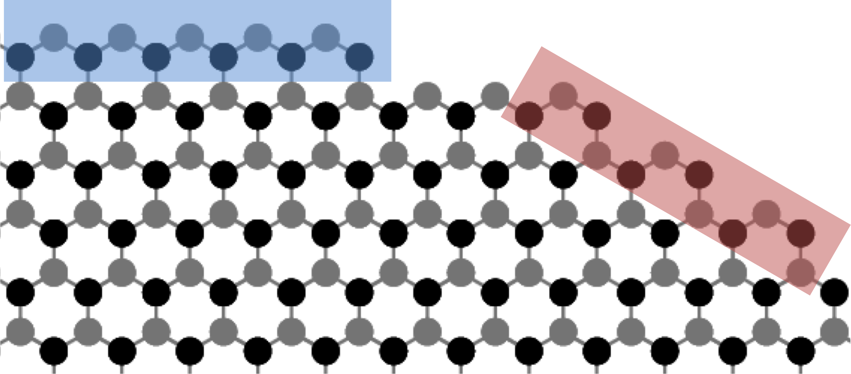
Figure 1: A magnified view of a boundary on a graphene flake. The orientation of the cut relative to the orientation of the lattice can produce two edge types, zigzag (highlighted in blue) and armchair (highlighted in red). The two sublattices of the unit cell are indicated in black (A-sublattice) and grey (B-sublattice).

We study finite graphene systems extracted from an infinite honeycomb lattice. A filter is applied to remove atom sites which are attached to only one other atom site, and to bridge under-coordinated sites whose $\pi$ orbitals would strongly overlap. As a result, each edge is either a pure zig-zag, armchair, or mixed boundary, as shown in Fig. 1. Recent studies have suggested that under certain circumstances, zig-zag edges reconstruct to form a 5-7 chain(Re-ZagDFT, ), however their scattering properties appear to be identical to regular zig-zag boundaries (Re-ZagWimmer, ). We have elected not to incorporate these features and leave them to future work.

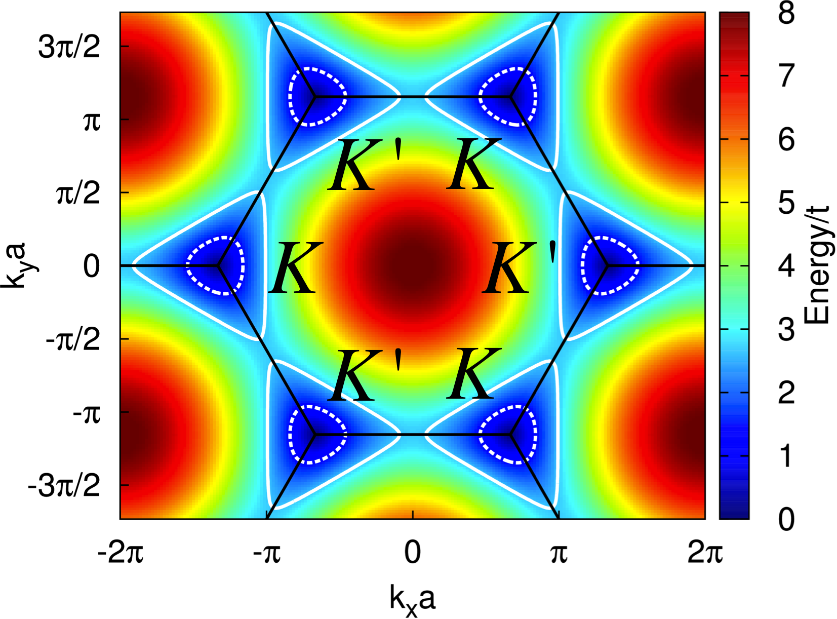
Figure 2: The two-dimensional dispersion relation for graphene demonstrates the two inequivalent valleys as cones where the edges of the Brillouin Zones (black lines) meet. Dashed white lines indicate the one-dimensional dispersion surface at $E=0.5t$, while solid white lines indicate $E=0.98t$, demonstrating extreme triagonal warping.

The band structure for graphene prominently features the two inequivalent $K^{\prime}$ and $K$ valleys in the energy range of $-t\leq E\leq t$(castro-neto, ), as can be seen in Fig. 2. At energies close to the Dirac point $E=0$, these valleys exhibit a linear dispersion relation and the electron behaves as a four-component spinor Dirac particle (two pseudo-spins, and two traditional spins). Using the creation operators $\mathbf{a}^{\dagger}$ and $\mathbf{b}^{\dagger}$ on the A- and B-sublattices respectively (see Fig. 1), the two pseudospinors can be written as

$$\psi_{\pm,\mathbf{K}}(\mathbf{k}) = \frac{1}{\sqrt{2}}\left(e^{-i\theta_{\mathbf{k}}/2}\mathbf{a}^{\dagger}\pm e^{i\theta_{\mathbf{k}}/2}\mathbf{b}^{\dagger}\right)$$ (7)

$$\psi_{\pm,\mathbf{K}^{\prime}}(\mathbf{k}) = \frac{1}{\sqrt{2}}\left(e^{i\theta_{\mathbf{k}}/2}\mathbf{a}^{\dagger}\pm e^{-i\theta_{\mathbf{k}}/2}\mathbf{b}^{\dagger}\right),$$ (8)

where $\theta_{\mathbf{k}}=\arctan\left(\frac{q_{x}}{q_{y}}\right)$, $\mathbf{q}=\mathbf{k}-\mathbf{K}^{(\prime)}$ and the $\pm$ signs indicate whether the positive- or negative-energy solutions are being used(castro-neto, ). While the linear dispersion no longer applies at energies above $\sim 0.4t$, the Dirac basis remains useful as a means of describing the classical dynamics of graphene throughout the energy range $-t\leq E\leq t$. States near the Dirac point and at the upper edge of this spectrum are examined in this paper.

It might be tempting to obtain a representation of either valley in a graphene wavefunction by subtracting off a plane wave whose wavevector corresponds to the origin of either $K$ or $K^{\prime}$ valley, leaving behind the residual $\mathbf{q}=\mathbf{k}-\mathbf{K}^{(\prime)}$. However, this approach only works when quasiparticles are present in only one valley, an assumption that cannot be generally guaranteed.

On the other hand, since wavevectors for each valley are sufficiently separated in $k$-space, the Husimi projection can distinguish each valley unambiguously for most momentum uncertainties. Because the valleys are part of the same band, a scattered quasiparticle from one valley can emerge in the other(ashcroft-and-mermin, ). When this occurs, the Husimi map shows quasiparticles in one valley funneling into a drain, and quasiparticles in the other valley emitting from a source at the same point, leaving behind a signature for inter-valley scattering.

Between $-t<E<t$, the Fermi energy contours warp from a circular shape near the Dirac point to trigonal contours, which emphasize three directions for each valley in the distribution of group velocities $v_{g}=\Delta_{\mathbf{k}}E\left(\mathbf{k}\right)$. As a result, the magnitude of the wavevector $\mathbf{q}=\mathbf{k}-\mathbf{K}^{(\prime)}$ depends on its orientation: It is bounded above by

$$q_{\text{up}}=\frac{2}{a}\cos^{-1}\left[\frac{1}{4t}\left(E+t+\sqrt{-3E^{2}-6Et+9t^{2}}\right)\right],$$ (9)

and from below by

$$q_{\text{low}}=\frac{2}{a}\cos^{-1}\left[\frac{1}{4t}\left(-E+t+\sqrt{-3E^{2}+6Et+9t^{2}}\right)\right].$$ (10)

When characterizing the momentum uncertainty, we use the average of these two quantities.

III Results

III.1 States Away from the Dirac Point

\begin{overpic}[width=184.28981pt]{three_stadia.png}\put(-4.0,97.0){(a)}\put(-4.0,62.0){(b)}\put(-4.0,30.0){(c)}\end{overpic}

Figure 3: The Husimi map for three eigenstates of the closed graphene stadium billiard with 20270 orbital sites at energy $E=0.974t\text{(a)},0.964t\text{(b)},\text{ and }0.951t\text{(c)}$. All three calculations use coherent states with relative uncertainty $\Delta k/k=30\%$, whose breadth is indicated by the double arrows on the right. Only the upper-right quarter of each stadia is shown. At left, the multi-modal analysis for the $K^{\prime}$ valley, and at right the wavefunction representation. The divergence of the Husimi map is indicated in green (red) to for positive (negative) values. Angular deflection is indicated in blue (Eq. 12). Red boxes indicate the magnified views in Fig. 4.

\begin{overpic}[width=184.28981pt]{three_stadia_zoom-in_no_label.png}\put(0.0,64.5){(a)}\put(34.0,64.5){(b)}\put(68.0,64.5){(c)}\end{overpic}

Figure 4: Magnified views of the divergence and angular deflection in Fig. 3 (red boxes). The sources and drains in the $K^{\prime}$-valley Husimi map are actually inter-valley scattering points, which occur along non zig-zag boundaries. In contrast, points of angular deflection that are not sources or drains correspond to intra-valley scatterers and occur along pure or nearly-pure zig-zag boundaries.

Fig. 3 shows Husimi maps for three eigenstates of a large closed-system stadium billiard with 20270 orbital sites at energies of $E=0.974t\text{(a)},0.964t\text{(b)},\text{ and }0.951t\text{(c)}$. We have chosen these states because they exhibit very clear linear trajectories. At energies close to $E=t$, trajectories exhibit pronounced trigonal warping, as seen by the three preferred directions. While the classical trajectories are obvious in the wavefunction itself, the Husimi map identifies the direction of each trajectory with respect to each valley.

The presence a few dominant classical paths in each wavefunction in Fig. 3 allows us to infer the relationship between boundary types and scattering among the two Dirac valleys. When a quasiparticle in one valley scatters into the other, it appears in the Husimi map as drain. We can measure this by summing the divergence for all angles in the Husimi map as

$$Q_{\text{div.}}\left(\mathbf{r};\Psi\right)=\int D(\mathbf{r},\mathbf{k};\Psi)\left|\boldsymbol{\nabla}_{\mathbf{k}}E\left(\mathbf{k}\right)\right|d^{d}k^{\prime},$$ (11)

where $D(\mathbf{r},\mathbf{k};\Psi)$ is defined as the divergence of the Husimi map for one wavevector $\mathbf{k}$,

$$D(\mathbf{r},\mathbf{k};\Psi) = \int\sum_{i=1}^{d}\frac{\text{Hu}\left(\mathbf{k},\mathbf{r}^{\prime};\Psi\right)-\text{Hu}\left(\mathbf{k},\mathbf{r};\Psi\right)}{\left(\mathbf{r}^{\prime}-\mathbf{r}\right)\cdot\mathbf{e}_{i}}$$ (12)

$$\times\exp\left[\frac{\left(\mathbf{r}^{\prime}-\mathbf{r}\right)^{2}}{2\sigma^{2}}\right]d^{d}r^{\prime},$$

where we sum over the $d$ orthogonal dimensions each associated with unit vector $\mathbf{e}_{i}$. The divergence in the $K^{\prime}$ valley, seen in green and red (for positive and negative values, respectively) in Figs. 3 and 4, shows that the scattering points all lie along non-zig-zag boundaries. Plots for the $K$ valley (not shown) are inverted, corroborating the time-reversal symmetry relationship between the two valleys.

On the other hand, when a quasiparticle in one valley reflects off a boundary but does not scatter into the other valley, the divergence is zero, but the reflection can still be measured in the angular deflection of the Husimi map,

$$Q_{\text{ang.}}\left(\mathbf{r};\Psi\right)=\int\left|D_{\text{abs.}}(\mathbf{r},\mathbf{k};\Psi)\boldsymbol{\nabla}_{\mathbf{k}}E\left(\mathbf{k}\right)\right|d^{d}k.$$ (13)

$D_{\text{abs.}}(\mathbf{r},\mathbf{k};\Psi)$ is defined as the absolute divergence of the Husimi function for one particular trajectory angle with a wavevector $\mathbf{k}$,

$$D_{\text{abs.}}(\mathbf{r},\mathbf{k};\Psi) = \int\sum_{i=1}^{d}\left|\frac{\text{Hu}\left(\mathbf{k},\mathbf{r}^{\prime};\Psi\right)-\text{Hu}\left(\mathbf{k},\mathbf{r};\Psi\right)}{\left(\mathbf{r}^{\prime}-\mathbf{r}\right)\cdot\mathbf{e}_{i}}\right|$$ (14)

$$\times\exp\left[\frac{\left(\mathbf{r}^{\prime}-\mathbf{r}\right)^{2}}{2\sigma^{2}}\right]d^{d}r^{\prime}.$$

As a result, boundary points with large angular deflection are either inter-valley or intra-valley scatterers depending on the magnitude of divergence at each point.

In Figs. 3 and 4, we plot the angular deflection in blue to compare to the divergence in green and red. Using this information, we can determine that for the wavefunction in Fig. 3a, all boundary scattering points are inter-valley scatterers, since all points of angular deflection exhibit divergence. The wavefunction in Fig. 3b, on the other hand, only exhibits divergence along the vertical sides of the stadium billiard: the horizontal top edge exhibits strong angular deflection but no divergence, and constitutes an intra-valley scatterer. Examining the magnified views in Figs. 4a and 4b, we see that inter-valley scatterers correspond to armchair edges, and the intra-valley scatterers belong to zig-zag edges, corroborating the findings at the Dirac point by Akhmerov and Beenakker(BeenakkerBC, ). Similar points of scattering can also be found in Figs. 3c and 4c.

Because of the time-reversal relationship between the two valleys, the severe restriction on group velocities, and the placement of zig-zag and armchair boundaries, no path at these energies exists without interacting with an inter-valley scatterer (data not shown). By comparison, it is not only possible but common to find states near the Dirac point that exhibit the opposite: all boundary conditions which are expressed belong to only intra-valley scatterers (See Sec. III.2).

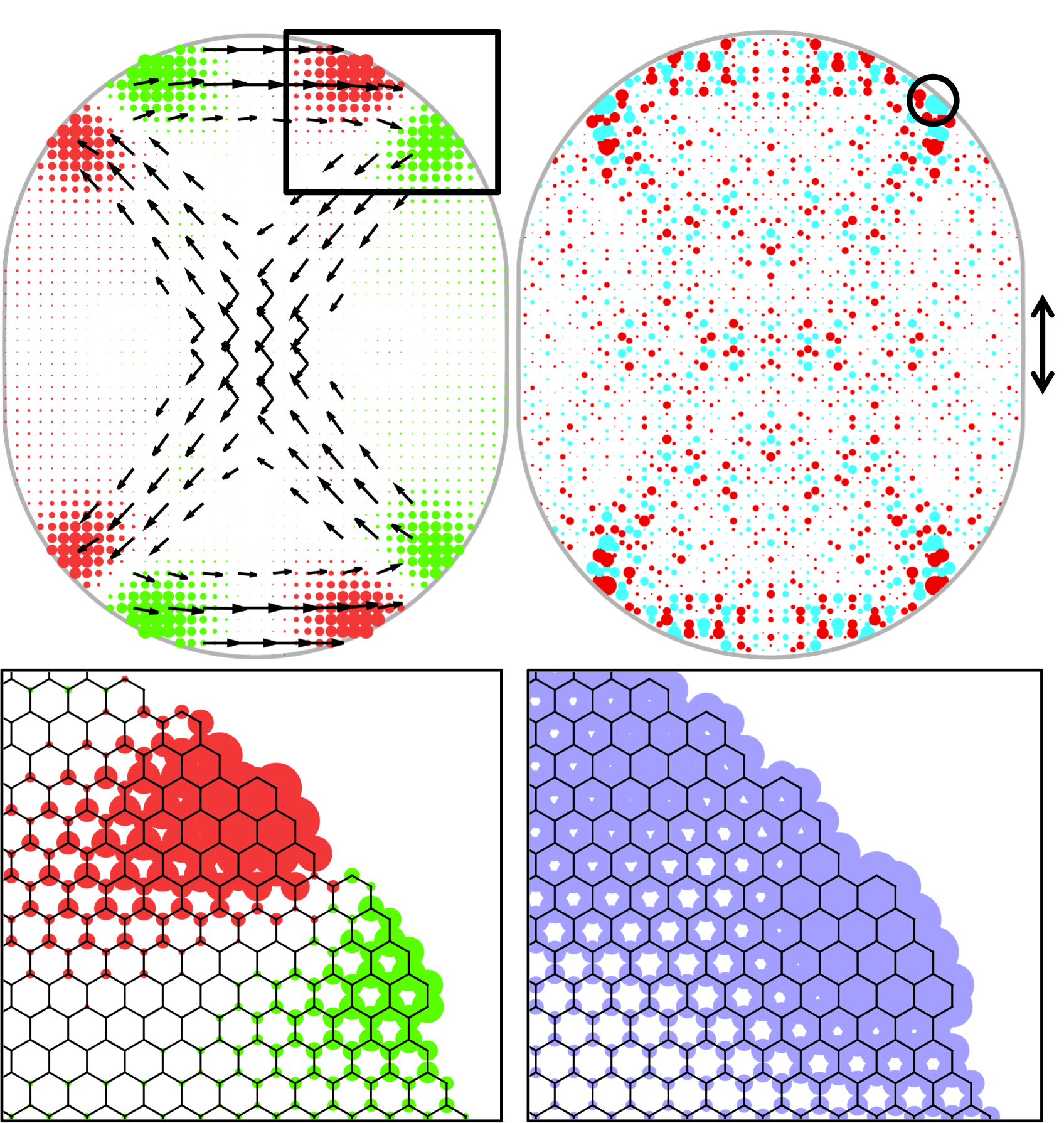
Figure 5: A closed-system eigenstate at $E=0.72t$ for the smaller graphene stadium. At top, the filtered Multi-Modal analysis is with relative momentum uncertainty $\Delta k/k=30\%$ along with the wavefunction (right). The spread of the coherent state is indicated by the double arrows. At bottom, higher-resolution calculations of the divergence (green for positive, red for negative) and the angular deflection (blue) are shown against the graphene structure. The black circle indicates where the system boundary is perturbed in the original paper(Huang-PRL-Scars, ) as discussed in Section III.3.

In comparison to Fig. 3, the eigenstate of the much smaller graphene stadium system in Fig. 5 does not appear to show isolated trajectories in its wavefunction representation. This is not surprising since this system can only accommodate five deBroglie wavelengths vertically, and three horizontally, severely restricting its ability to resolve such trajectories. However, clear self-retracing trajectories are quite visible in the Husimi map in Figs. 5, with evident sources and drains inhabiting the boundary, showing that the Husimi map can yield a semiclassical interpretation of the dynamics of the states not possible from just the wavefunction of the system. Moreover, because the paths indicated by the Husimi map marshal the electron away from lateral boundaries, where leads connect to produce the open system in Sec. III.3, the Husimi map helps us understand the role this state plays in forming a long-lived resonance in the open system.

In both Figs. 3 and 5, wavefunctions in graphene away from the Dirac point are linked to valley switching classical ray paths which bounce back and forth along straight lines. These wavefunction enhancements are not strictly scars(PhysRevLett.53.1515, ), as first suggested by Huang et al.(Huang-PRL-Scars, ), since scars are generated by unstable classical periodic orbits in the analogous classical limit (group velocity) system. Instead, the wavefunction structures are more likely normal quantum confinement to stable zones in classical phase space constrained by group-velocity warping at these energies.

III.2 States Near the Dirac Point

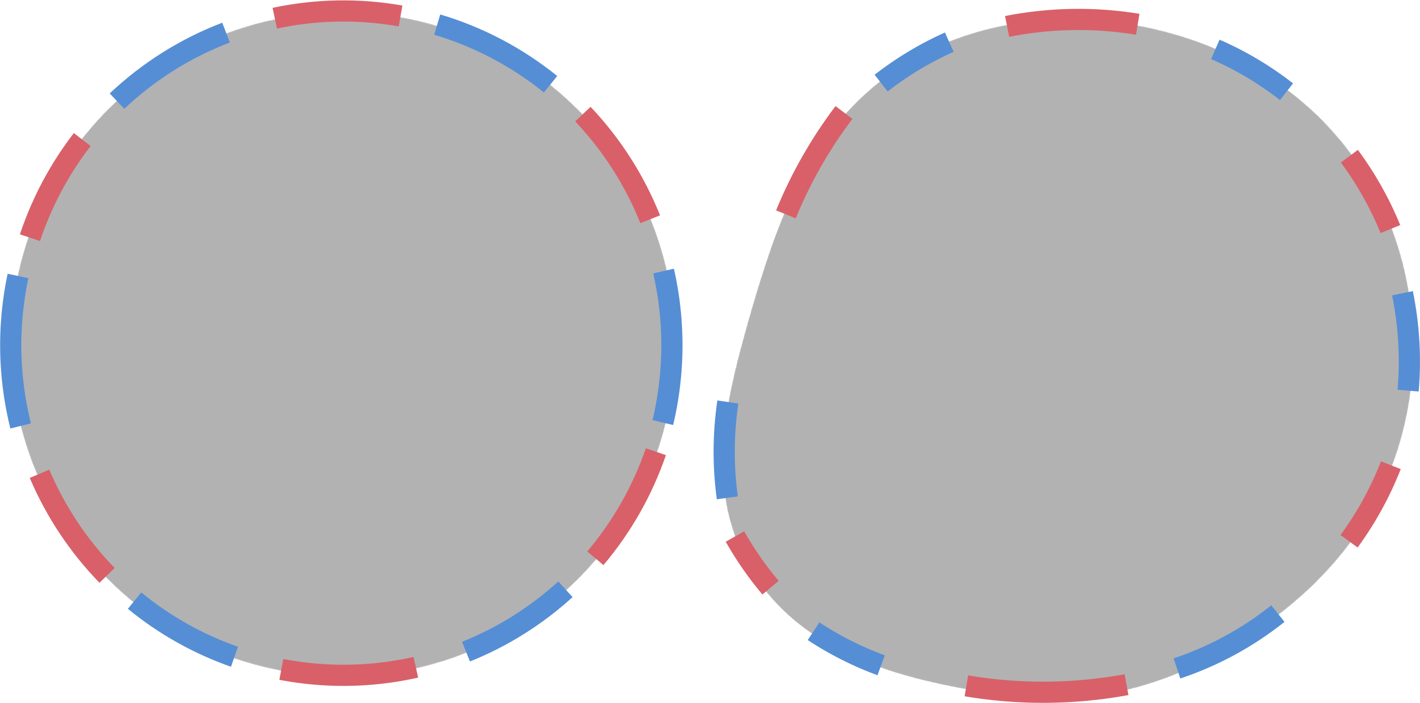
Figure 6: Schematic indicating the locations of armchair (blue) and zig-zag (red) edges in the circular system (left) and the Wimmer system (right).

\begin{overpic}[width=216.81pt]{four_circles_narrow.png}\put(1.0,96.5){(a)}\put(1.0,73.0){(b)}\put(1.0,48.0){(c)}\put(1.0,23.5){(d)}\end{overpic}

Figure 7: Low-energy graphene states require additional tools to fully grasp the classical dynamics. The Husimi map for the $K^{\prime}$-valley is plotted for four eigenstates of a closed circular system with 71934 orbital sites at energies around $E=0.2t$. All three calculations use coherent states with relative uncertainty $\Delta k/k=20\%$, with breadth indicated by the double arrows on the right. From left-to-right: the Husimi flux, multi-modal analysis, and the wavefunction. The divergence of the Husimi flux is indicated in green (red) for positive (negative) values. In blue, the angular deflection.

We now explore the properties of low-energy closed-system states in graphene, using the circular graphene flake and the distorted circular flake introduced by Wimmer et al.(Wimmer-Robusteness, ). The latter geometry was chosen because its dynamics are chaotic and sensitive to the placement of armchair and zig-zag boundaries, which shift as a result of the distortion. We indicate the two boundary types for both geometries in Fig. 6..

In the continuous system, the Fermi wavevector grows with the square-root of the energy, but in graphene, the effective wavevector $\mathbf{q}=\mathbf{k}-\mathbf{K}^{(\prime)}$ grows linearly. As a result, the deBroglie wavelength is much larger for the graphene system than for the continuous system at similar energy scales, making it difficult to conduct calculations with sufficient structure in the wavefunction. Consequently, we examine states at energies away from the Dirac point to bring calculations within a reasonable scope. (For instance, we have selected a system size under 100,000 orbital sites to facilitate replication of our results). Since trigonal warping becomes significant above $E=0.4t$, we have selected the energy of $0.2t$ for all states in our analysis to maximize the number of wavelengths within a small graphene system while maintaining the same physics from energies closer to the Dirac point.

Fig. 7 shows four eigenstates of the circular graphene flake. Like the free-particle circular well, eigenstates of the graphene circular flake resemble eigenstates of the angular momentum operator (see Mason et al.(Mason-Husimi-Continuous, ) for direct comparisons and Husimi maps). For instance, the wavefunctions in Figs. 7a-b are radial-dominant, while the wavefunction in Fig. 7d is angular-dominant. These observations carry over to the dynamics of the wavefunctions revealed by the multi-modal analysis for the $K^{\prime}$ valley, which shows radially-oriented paths in Figs. 7a-b and circular paths skimming the boundary in Fig. 7d. Fig. 7c shows a state with a mixture of radial and angular components; in the multi-modal analysis, this appears as straight paths between boundary points highlighted by the angular deflection.

Unlike free-particle circular wells, however, the lattice sampling on the honeycomb lattice breaks circular symmetry and replaces it with six-fold symmetry. Because eigenstates of the system emphasize certain boundary conditions, the manner in which each state establishes itself strongly varies. For instance, the two radial-dominant states in Figs. 7a-b exhibit intravalley (a) or intervalley (b) scattering. Accordingly, the locations where the rays terminate on the boundary correlate with zig-zag and armchair boundaries respectively. The wider spread in angular deflection in Fig. 7a corroborates Akhmerov and Beenakker(BeenakkerBC, ), showing that that intravalley scattering occurs over a larger set of boundaries than intervalley scattering.

Because each valley reflects back to itself in Fig. 7a, there is no net flow of either valley in the bulk of the system. As a result, the multi-modal analysis shows counter-propagating flows, and the Husimi flux (Eq. 5) is zero except at the center, where slight offsets in trajectories form characteristic vortices. In Fig. 7b, on the other hand, each ray in the wavefunction is associated with a distinct source and drain, which is evident in both the multi-modal analysis and the Husimi flux.

In Figs. 7c-d, the locations of sources and drains for the $K^{\prime}$ valley are reversed from Fig. 7b. However, the roles that inter-valley scattering play in these states is less clear; rather, inter- and intra-valley scattering dominate these wavefunctions. In Fig. 7c, this can been by the emphasis of angular deflection along the zig-zag boundaries, which do not show any divergence. In Fig. 7d, even though the wavefunction and the multi-modal analysis clearly emphasize a classical path that skims the boundary, the path actually flips between each valley each time it encounters an inter-valley scatterer. For both states, the various trajectories merge to form vortices in the Husimi flux, with sources and drains at armchair edges.

\begin{overpic}[width=216.81pt]{beenakker_without_hybrids.png}\put(1.0,66.0){(a)}\put(1.0,33.0){(b)}\end{overpic}

Figure 8: In parts (a) and (b), the same information is plotted as in Fig. 7, but for the Wimmer system (see Fig. 6), with 96425 orbital sites. These states also have energies near $E=0.2t$ and are represented by coherent states of uncertainty $\Delta k/k=20\%$ with breadth indicated by the double arrows.

When the circular flake is distorted, as in the Wimmer system (Figs. 6 and 8), inter- and intra-valley scatterers are re-arranged and re-sized as a function of the local radius of curvature of the boundary.

Figs. 8a-b show two eigenstates of the Wimmer system. The boundary conditions for these states most closely resemble Fig. 5, since sources and drains appear next to each other. This is a signature of mixed scattering – both inter- and intra-valley scattering occur in various proportions at these points. For example, the multi-modal analysis in Fig. 8a shows a triangular path, but not all legs of the triangle are equally strong, corresponding to various degrees of absorption and reflection at each scattering point which can be seen in the divergence.

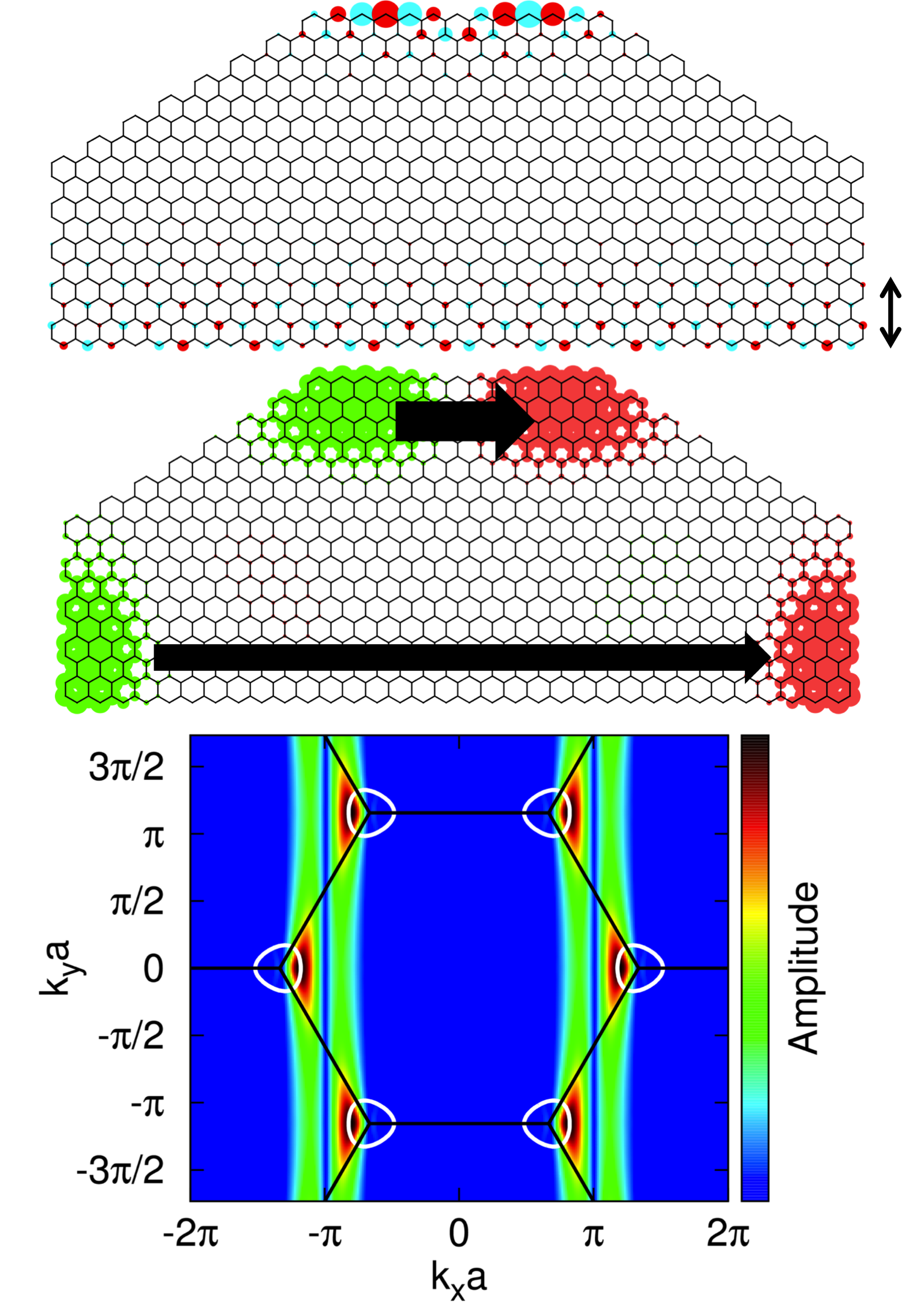
Figure 9: An extremely small “rooftop” graphene flake at energy $E=0.0015735t$ showing two edge states at the top and bottom boundaries which tunnel into each other. At top, the full wavefunction, at middle, divergence is indicated in green and red, and a schematic of the Husimi flux for the $K^{\prime}$ valley is shown. At bottom, the Fourier transform of the state is shown, with the contour line used to generate the Husimi map in white, set at an arbitrary energy in order to maximize the intersection of the contour with the Fourier-transform amplitude. The spread of the wavepacket used to generate this map is indicated by the double arrows.

Edge-states are a set of zero-energy surface states that are strongly localized to zig-zag boundaries and potentially long-lived(castro-neto, ), and since they can be used as modes of transport(Wimmer-Spin-Currents-Rough-Nanoribbons, ; Wimmer-Spin-Transport, ) and be strongly spin-polarized(KaxirasNanoFlakes, ; WeiLi, ), they have been proposed a candidate for spin-tronics devices(castro-neto, ; KaxirasNanoFlakes, ; Wimmer-Spin-Currents-Rough-Nanoribbons, ; Wimmer-Spin-Transport, ; WeiLi, ). But because edge states exhibit a different dispersion relation than the two valleys in the bulk, they cannot be “sensed” by the $K^{\prime}$ or $K$ valley Husimi projections. Instead, the Husimi map can be generated using wavevectors appropriate to the edge states, which shows them as standing waves on the surface (see Fig. 9). As noted in Wimmer et al.(Wimmer-Robusteness, ), it is possible for edge states to tunnel into each other using bulk states as a medium, but we have found that $K^{\prime}$ or $K$ valley Husimi maps of bulk states which hybridize with them are indistinguishable from their non-hybridized counterparts

III.3 Fano Resonance

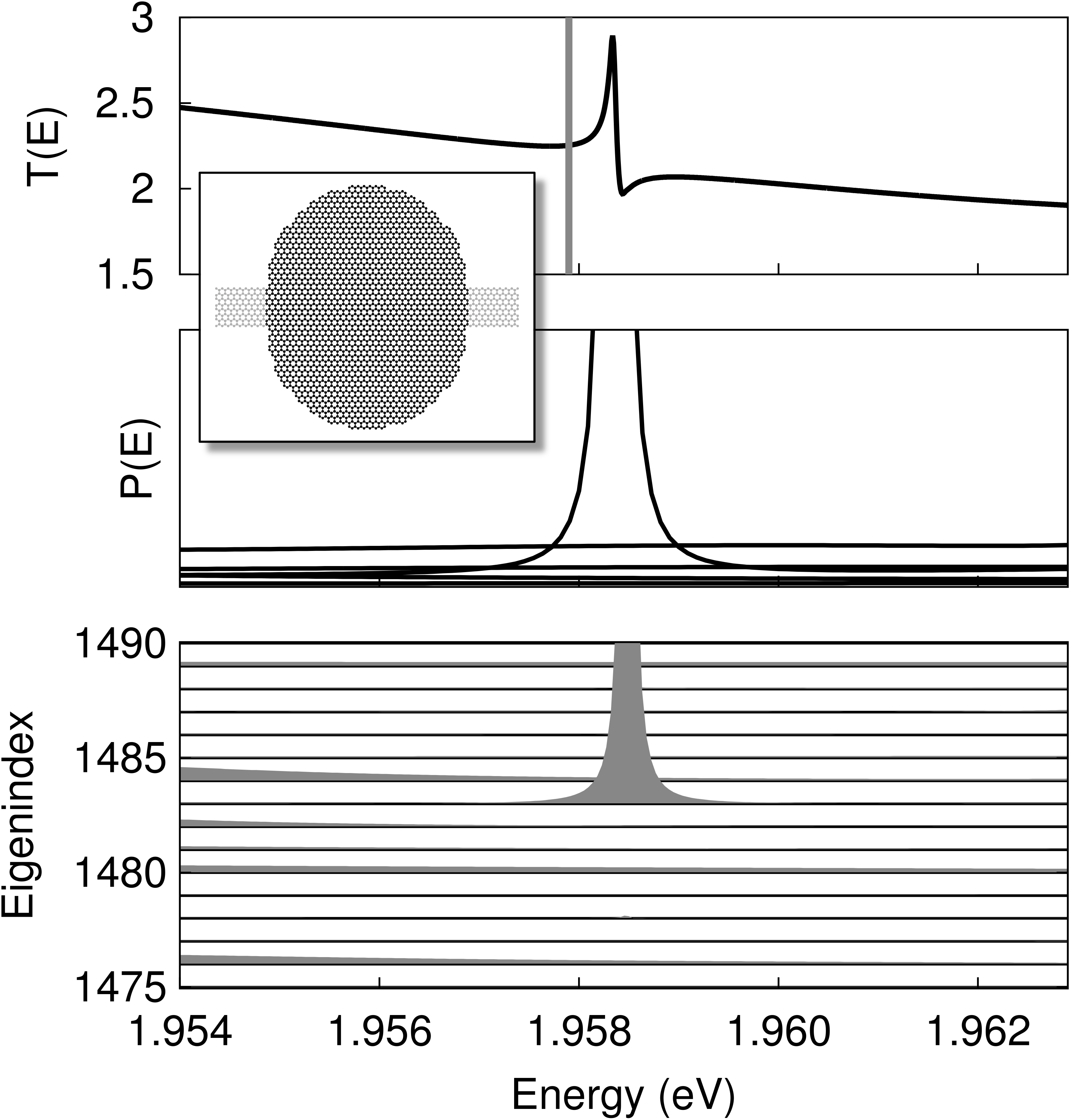
Figure 10: System properties of the scattering density matrix $\rho$ around the Fano resonance centered at $E=1.9582\text{eV}$ for the open system in the inset. Top: The transmission profile across the two leads, with the closed-system eigenstate energy at $E=1.9579\text{eV}$, corresponding to the eigenstate at index 1483 (below), indicated by the vertical grey line. Middle: Diagonalizing the density matrix produces a handful of non-trivial scattering wavefunctions in its eigenvectors. The eigenvalues of these vectors, which correspond to their measurement probability, are graphed. The wavefunction associated with the closed-system eigenstate hybridizing with the direct channel peaks strongly around the Fano resonance. Bottom: The density matrix is projected onto the closed-system eigenstates, showing that eigenstate 1483 strongly peaks at the Fano resonance.

This section addresses Fano resonance(fano-original, ) in graphene systems, a conductance phenomenon that occurs as a result of interference between a direct state (conductance channel) and a quasi-bound indirect state similar to the eigenstates this paper has examined. Fano resonances are an ideal case study for the Husimi map, not only because they are ubiquitous in theory(ferry-pointer-states, ; Munoz-Rojas2006, ) and experiments(Fano-Experiment2, ; Fano-Experiment, ; Fano-Experiment3, ), but also because their behavior is well-understood(datta, ; mesoscopicbook, ; ferrybook, ; transport-book2, ; dots-transport-book, ; datta2, ; fano-review, ). However, Fano resonances in graphene quantum dots are less well characterized(Wimmer-Energy-Levels, ; Huang-Trans-Scar, ; Huang-Open-Dots, ; Huang-Cond-Fluc, ) and lack a comprehensive theory relating boundary conditions to bulk state behavior in graphene.

To study Fano resonance, we first compute a scattering wavefunction using the recursive numerical Green’s function method described in Mason et al.(mason, ). This method produces a scattering density matrix $\rho$, which is diagonalized. Each eigenvector corresponds to a scattering wavefunction, which has an associated eigenvalue indicating its measurement probability (Fig. 10, middle). We focus on the resonance study in Huang et al.(Huang-PRL-Scars, ).

The resonance in Fig. 10 is associated with the eigenstate from Fig. 5 of the closed billiard system. This eigenstate couples only weakly to leads which are attached at its sides (shown in the inset of Fig. 10). This makes it possible for a scattering electron to enter the system through a direct channel but then become trapped in a quasi-bound state related to the eigenstate, causing the density of states projected onto the eigenstate to strongly peak near its eigenenergy (Fig. 10, bottom). As the system energy sweeps across the eigenenergy, the phase of the eigenstate component shifts through $\pi$, causing it to interfere negatively and then positively with the direct channel, giving rise to the distinctive Fano curve (Fig. 10, top). As a result, the scattering wavefunction with the largest measurement probability is in fact a hybridized state between the closed-system eigenstate and the direct channel, and its probability peaks around an energy near, but not exactly the same as, the eigenstate energy (Fig. 10, middle). The shift in energy arises as a perturbation from the leads.

For closed graphene systems, the two valleys satisfy time-reversal symmetry as an analytical consequence of lattice sampling on the honeycomb lattice. As a result, trajectories in one valley are exactly reversed from the other valley, in analogy with free-particle systems where opposing trajectories cancel each other produce zero flux. This observation allows us to remove the time-reversal symmetry of a scattering wavefunction by summing the projections for both valleys, revealing the time-reversal asymmetric part of the wavefunction.

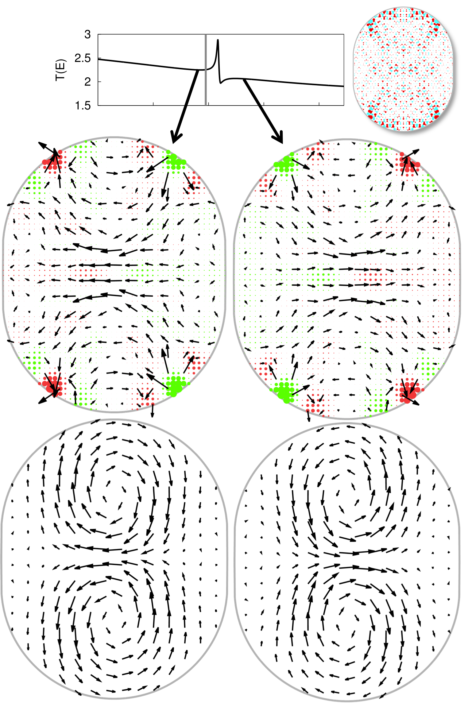
Figure 11: Above and below the Fano resonance in Figs. 10 (inset), the time-reversal symmetry between the $K$ and $K^{\prime}$ valleys is lifted, making it possible to add the Husimi flux for both valleys to measure valley-polarized current. Above, the Husimi flux maps of both valleys are added for the scattering wavefunction at energies $E=1.9582t$ and $1.9586t$, with $\Delta k/k=30\%$. Below, the probability flux, convolved with a Gaussian kernel of the same size as the coherent state. At energies this close to resonance, the wavefunction does not visually change from the closed-system eigenstate in the inset, but the residual current that occurs near these resonances switches direction across resonance.

Fig. 11 shows the results of adding the Husimi flux maps of both valleys at two energies, below and above resonance. We find sources and drains in the summed Husimi flux map at the corners of the system where the classical paths of the $K^{\prime}$-valley Husimi map (Fig. 5) reflect off the system boundary.

To understand why, we consider that during transmission, quasiparticles enter from the left incoming lead and exit through the right outgoing lead. However, near resonance, the wavefunction is strongly weighted by the closed-system eigenstate, which has no net quasiparticle current. Husimi maps for either valley also reflect this fact: they are indistinguishable from the Husimi maps of the closed-system eigenstate in Fig. 5, and the two valleys are inverse images of each other.

But the Husimi maps for the two valleys don’t exactly cancel each other out. When we add them together to reveal the time-reversal asymmetric behavior of the wavefunction, the residual shows sources and drains of net quasiparticle flow which are strongly related to the Husimi maps for each valley, and do not show left-to-right transmission. Instead, the summed Husimi flux map shows the influence of transmission on the strongly-emphasized classical paths underlying the closed-system eigenstate.

To compare the summed Husimi flux map to the traditional flux, we consider the probability flow between two adjacent carbon atom sites called the bond current, defined as

$$j_{i\rightarrow j}=\frac{4e}{h}\text{Im}\left[H_{ij}G_{ij}^{n}(E)\right],$$ (15)

where $H_{ij}$ and $G_{ij}^{n}(E)$ are the off-diagonal components of the Hamiltonian and the electron correlation function between orbital sites $i$ and $j$(datta, ; graphene-bond-current2, ). The electron correlation function is proportional to the density matrix, but in our calculations, we examine just one scattering state, so that $G_{ij}^{n}\propto\psi_{i}\psi_{j}^{\ast}$ where $\psi_{i}$ is the scattering state probability amplitude at orbital site $i$. We can obtain a finite-difference analog of the continuum flux operator by defining

$$\mathbf{j}_{i}=\sum_{j}j_{i\rightarrow j}\frac{\mathbf{r}_{j}-\mathbf{r}_{i}}{\left|\mathbf{r}_{j}-\mathbf{r}_{i}\right|^{2}},$$ (16)

which computes the vector sum of each bond current associated with a given orbital(graphene-bond-current, ).

Convolving the flux defined in Eq. 16 with a Gaussian kernel of the same spread as the coherent state used to generate the Husimi map creates an analog to the Husimi flux, except that the convolved flux does not distinguish among valleys. We show the convolved flux at the bottom of Fig. 11, and find that it forms vortices which correlates with the summed Husimi flux maps, and also fails to show the left-to-right flow responsible for transmission.

This behavior is directly analogous to flux in continuum systems, where flux vortices above and below resonance show local variations of flow but not the left-to-right drift velocity responsible for transmission. We can recover the left-to-right flow only by examining the system at larger scales using larger Gaussian spreads (not shown)(Mason-Husimi-Continuous, ). Because of the $\pi$ phase shift of the indirect channel across resonance, local flows reverse direction above and below resonance, but they do not affect the left-to-right flow at larger scales except exactly on resonance.

The stable orbits that underly the indirect channel, shown in Fig. 5, can be dramatically disturbed by slight modifications of the boundary where the classical paths reflect off the boundary. The original authors Huang et al.(Huang-PRL-Scars, ) examined the relationship between system symmetry and strength of the Fano resonances by slightly modifying the system boundary at the black circle in Fig. 5, and demonstrated that some resonances were drastically reduced by this modification.

We have chosen the resonance in this study because the Fano resonance profile associated with it was among the most-reduced as a result of their system modification, and our analysis provides a clear picture as to why: the system is perturbed precisely at the boundary where the eigenstate in Fig. 5 has the largest probability amplitude. With the semiclassical picture, we are able to add to this finding an intuitive understanding: by disturbing the reflection angle at the exact point where the two valleys scatter, each time the electron scatters off that point some of its probability leaves the stable orbit. The authors effectively introduced a leak into the orbit, reducing its lifetime and the strength of its resonance considerably.

IV Conclusions

We have examined the semiclassical behavior of graphene systems using a generalized technique that produces a vector field from projections onto coherent states, forming an infinitely tunable bridge between the large-scale Dirac effective field theory and the underlying atomistic model(castro-neto, ). We have used this technique, called the Husimi map, to examine the relationship between graphene boundary types and the classical dynamics of quasiparticles in each valley of the honeycomb dispersion relation, looking at states with energies both close to and far from the Dirac point. We have shown that closed-system eigenstates are associated with valley-polarized currents with zero net quasiparticle production. We show that Fano resonance are associated with an asymmetrical flow of quasiparticles strongly related to the valley-polarized currents of closed-system states, which has implications for applications in “valleytronic” devices(valleytronics, ). The ubiquity of this phenomenon in the systems we have studied suggests that they could appear in future experiments, and provides a motivation for further theoretical and experimental work.

- [1] A. K. Geim and K. S. Novoselov. The rise of graphene. Nature Materials, 6(3):183–191, 03 2007.
- [2] Melinda Y. Han, Barbaros Özyilmaz, Yuanbo Zhang, and Philip Kim. Energy band-gap engineering of graphene nanoribbons. Phys. Rev. Lett., 98:206805, May 2007.
- [3] K. S. Novoselov, Z. Jiang, Y. Zhang, S. V. Morozov, H. L. Stormer, U. Zeitler, J. C. Maan, G. S. Boebinger, P. Kim, and A. K. Geim. Room-temperature quantum hall effect in graphene. Science, 315(5817):1379, 2007.
- [4] Elena Stolyarova, Kwang Taeg Rim, Sunmin Ryu, Janina Maultzsch, Philip Kim, Louis E. Brus, Tony F. Heinz, Mark S. Hybertsen, and George W. Flynn. High-resolution scanning tunneling microscopy imaging of mesoscopic graphene sheets on an insulating surface. Proceedings of the National Academy of Sciences, 104(22):9209–9212, 2007.
- [5] G. M. Rutter, J. N. Crain, N. P. Guisinger, T. Li, P. N. First, and J. A. Stroscio. Scattering and interference in epitaxial graphene. Science, 317(5835):219–222, 2007.
- [6] Yuanbo Zhang, Victor W. Brar, Caglar Girit, Alex Zettl, and Michael F. Crommie. Origin of spatial charge inhomogeneity in graphene. Nat Phys, 5(10):722–726, 10 2009.
- [7] J Berezovsky, M F Borunda, E J Heller, and R M Westervelt. Imaging coherent transport in graphene (part i): mapping universal conductance fluctuations. Nanotechnology, 21(27):274013, 2010.
- [8] Jesse Berezovsky and Robert M Westervelt. Imaging coherent transport in graphene (part ii): probing weak localization. Nanotechnology, 21(27):274014, 2010.
- [9] A. H. Castro Neto, F. Guinea, N. M. R. Peres, K. S. Novoselov, and A. K. Geim. The electronic properties of graphene. Rev. Mod. Phys., 81(1):109–162, Jan 2009.
- [10] Michael Wimmer, İnan ç Adagideli, Sava ş Berber, David Tománek, and Klaus Richter. Spin currents in rough graphene nanoribbons: Universal fluctuations and spin injection. Phys. Rev. Lett., 100(17):177207, May 2008.
- [11] Wei L. Wang, Sheng Meng, and Efthimios Kaxiras. Graphene nanoflakes with large spin. Nano Letters, 8(1):241–245, 2008. PMID: 18052302.
- [12] Michael Wimmer, Matthias Scheid, and Klaus Richter. Spin-polarized Quantum Transport in Mesoscopic Conductors: Computational Concepts and Physical Phenomena. arXiv:0803.3705, 2008.
- [13] Wei L. Wang, Oleg V. Yazyev, Sheng Meng, and Efthimios Kaxiras. Topological frustration in graphene nanoflakes: Magnetic order and spin logic devices. Phys. Rev. Lett., 102(15):157201, Apr 2009.
- [14] T. O. Wehling, K. S. Novoselov, S. V. Morozov, E. E. Vdovin, M. I. Katsnelson, A. K. Geim, and A. I. Lichtenstein. Molecular doping of graphene. Nano Letters, 8(1):173–177, 2008. PMID: 18085811.
- [15] Stephan Schnez, Johannes Güttinger, Magdalena Huefner, Christoph Stampfer, Klaus Ensslin, and Thomas Ihn. Imaging localized states in graphene nanostructures. Phys. Rev. B, 82:165445, Oct 2010.
- [16] T. O. Wehling, A. V. Balatsky, M. I. Katsnelson, A. I. Lichtenstein, K. Scharnberg, and R. Wiesendanger. Local electronic signatures of impurity states in graphene. Phys. Rev. B, 75:125425, Mar 2007.
- [17] L. Simon, C. Bena, F. Vonau, D. Aubel, H. Nasrallah, M. Habar, and J. C. Peruchetti. Symmetry of standing waves generated by a point defect in epitaxial graphene. The European Physical Journal B - Condensed Matter and Complex Systems, 69:351–355, 2009. 10.1140/epjb/e2009-00142-3.
- [18] H. Amara, S. Latil, V. Meunier, Ph. Lambin, and J.-C. Charlier. Scanning tunneling microscopy fingerprints of point defects in graphene: A theoretical prediction. Phys. Rev. B, 76:115423, Sep 2007.
- [19] M.I Katsnelson and A.K Geim. Electron scattering on microscopic corrugations in graphene. Philosophical Transactions of the Royal Society A: Mathematical, Physical and Engineering Sciences, 366(1863):195–204, 2008.
- [20] Pekka Koskinen, Sami Malola, and Hannu Häkkinen. Evidence for graphene edges beyond zigzag and armchair. Phys. Rev. B, 80:073401, Aug 2009.
- [21] Jifa Tian, Helin Cao, Wei Wu, Qingkai Yu, and Yong P. Chen. Direct imaging of graphene edges: Atomic structure and electronic scattering. Nano Letters, 11(9):3663–3668, 2011.
- [22] Kyle A. Ritter and Joseph W. Lyding. The influence of edge structure on the electronic properties of graphene quantum dots and nanoribbons. Nature Materials, 8(3):235–242, 03 2009.
- [23] Douglas J. Mason, Mario F. Borunda, and Eric J. Heller. A semiclassical interpretation of probability flux. (unpublished) arXiv:1205.0291.
- [24] Douglas J. Mason, Mario F. Borunda, and Eric J. Heller. Extending the concept of probability flux. (unpublished) arXiv:1205.3708.
- [25] Douglas J. Mason, Mario Borunda, and Eric J. Heller. Husimi projections in lattices. (in preparation) arXiv:1206.1013, 2012.
- [26] Eric J. Heller. Bound-state eigenfunctions of classically chaotic hamiltonian systems: Scars of periodic orbits. Phys. Rev. Lett., 53(16):1515–1518, Oct 1984.
- [27] Liang Huang, Ying-Cheng Lai, David Ferry, Stephen Goodnick, and Richard Akis. Relativistic Quantum Scars. Phys. Rev. Lett., 103(5):1–4, July 2009.
- [28] U. Fano. Effects of configuration interaction on intensities and phase shifts. Phys. Rev., 124(6):1866–1878, Dec 1961.
- [29] David K. Ferry, Jonathan P. Bird, Richard Akis, David P. Pivin Jr., Kevin M. Connolly, Koji Ishibashi, Yoshinobu Aoyagi, Takuo Sugano, and Yuichi Ochiai. Quantum transport in single and multiple quantum dots. Jpn. J. Appl. Phys., 36(Part 1, No. 6B):3944–3950, 1997.
- [30] Andrey E. Miroshnichenko, Sergej Flach, and Yuri S. Kivshar. Fano resonances in nanoscale structures. Rev. Mod. Phys., 82:2257–2298, Aug 2010.
- [31] Pekka Koskinen, Sami Malola, and Hannu Häkkinen. Self-passivating edge reconstructions of graphene. Phys. Rev. Lett., 101:115502, Sep 2008.
- [32] J. A. M. van Ostaay, A. R. Akhmerov, C. W. J. Beenakker, and M. Wimmer. Dirac boundary condition at the reconstructed zigzag edge of graphene. Phys. Rev. B, 84:195434, Nov 2011.
- [33] N.W. Ashcroft and N.D. Mermin. Solid state physics. Holt-Saunders International Editions: Science : Physics. Holt, Rinehart and Winston, 1976.
- [34] A. R. Akhmerov and C. W. J. Beenakker. Boundary conditions for dirac fermions on a terminated honeycomb lattice. Phys. Rev. B, 77(8):085423, Feb 2008.
- [35] M. Wimmer, A. R. Akhmerov, and F. Guinea. Robustness of edge states in graphene quantum dots. Phys. Rev. B, 82(4):045409, Jul 2010.
- [36] D. K. Ferry, R. Akis, and J. P. Bird. Einselection in action: Decoherence and pointer states in open quantum dots. Phys. Rev. Lett., 93:026803, Jul 2004.
- [37] F. Muñoz Rojas, D. Jacob, J. Fernández-Rossier, and J. Palacios. Coherent transport in graphene nanoconstrictions. Physical Review B, 74(19):1–8, 2006.
- [38] J. Göres, D. Goldhaber-Gordon, S. Heemeyer, M. A. Kastner, Hadas Shtrikman, D. Mahalu, and U. Meirav. Fano resonances in electronic transport through a single-electron transistor. Phys. Rev. B, 62:2188–2194, Jul 2000.
- [39] Kensuke Kobayashi, Hisashi Aikawa, Akira Sano, Shingo Katsumoto, and Yasuhiro Iye. Fano resonance in a quantum wire with a side-coupled quantum dot. Phys. Rev. B, 70:035319, Jul 2004.
- [40] L. E. Calvet, J. P. Snyder, and W. Wernsdorfer. Fano resonance in electron transport through single dopant atoms. Phys. Rev. B, 83:205415, May 2011.
- [41] S. Datta. Electronic Transport in Mesoscopic Systems. Cambridge University Press, Cambridge, 1997.
- [42] L.L. Sohn, L.P. Kouwenhoven, and G. Schön. Mesoscopic electron transport. NATO ASI series: Applied sciences. Kluwer Academic Publishers, 1997.
- [43] D.K. Ferry and S.M. Goodnick. Transport in nanostructures. Cambridge Studies in Semiconductor Physics and Microelectronic Engineering. Cambridge University Press, 1999.
- [44] I.O. Kulik and R. Ellialtıoğlu. Quantum mesoscopic phenomena and mesoscopic devices in microelectronics. NATO science series: Mathematical and physical sciences. Kluwer Academic, 2000.
- [45] J.P. Bird. Electron transport in quantum dots. Kluwer Academic Publishers, 2003.
- [46] S. Datta. Quantum transport: atom to transistor. Cambridge University Press, 2005.
- [47] Jürgen Wurm, Adam Rycerz, İnan ç Adagideli, Michael Wimmer, Klaus Richter, and Harold U. Baranger. Symmetry classes in graphene quantum dots: Universal spectral statistics, weak localization, and conductance fluctuations. Phys. Rev. Lett., 102:056806, Feb 2009.
- [48] Liang Huang, Ying-Cheng Lai, David K Ferry, Richard Akis, and Stephen M Goodnick. Transmission and scarring in graphene quantum dots. Journal of Physics: Condensed Matter, 21(34):344203, 2009.
- [49] D K Ferry, L Huang, R Yang, Y-C Lai, and R Akis. Open quantum dots in graphene: Scaling relativistic pointer states. Journal of Physics: Conference Series, 220(1):012015, 2010.
- [50] Liang Huang, Rui Yang, and Ying-Cheng Lai. Geometry-dependent conductance oscillations in graphene quantum dots. EPL (Europhysics Letters), 94(5):58003, 2011.
- [51] Douglas J. Mason, David Prendergast, Jeffrey B. Neaton, and Eric J. Heller. Algorithm for efficient elastic transport calculations for arbitrary device geometries. Phys. Rev. B, 84:155401, Oct 2011.
- [52] Jie-Yun Yan, Ping Zhang, Bo Sun, Hai-Zhou Lu, Zhigang Wang, Suqing Duan, and Xian-Geng Zhao. Quantum blockade and loop current induced by a single lattice defect in graphene nanoribbons. Phys. Rev. B, 79:115403, Mar 2009.
- [53] L. P. Zârbo and B. K. Nikolić. Spatial distribution of local currents of massless dirac fermions in quantum transport through graphene nanoribbons. EPL (Europhysics Letters), 80(4):47001, 2007.
- [54] A. Rycerz, J. Tworzydlo, and C. W. J. Beenakker. Valley filter and valley valve in graphene. Nat Phys, 3(3):172–175, 03 2007.