Fluctuating surface-current formulation of radiative heat transfer for arbitrary geometries

Abstract

We describe a fluctuating surface-current formulation of radiative heat transfer, applicable to arbitrary geometries, that directly exploits standard, efficient, and sophisticated techniques from the boundary-element method. We validate as well as extend previous results for spheres and cylinders, and also compute the heat transfer in a more complicated geometry consisting of two interlocked rings. Finally, we demonstrate that the method can be readily adapted to compute the spatial distribution of heat flux on the surface of the interacting bodies.

Quantum and thermal fluctuations of charges in otherwise neutral bodies lead to stochastic electromagnetic (EM) fields everywhere in space. In non-equilibrium situations involving bodies at different temperatures, these fields mediate energy exchange from the hotter to the colder bodies, a process known as radiative heat transfer. Although the basic theoretical formalism for studying heat transfer was laid out decades ago Rytov et al. (1989); Polder and Van Hove (1971); Loomis and Maris (1994); Volokitin and Persson (2007); Zhang (2007); Basu et al. (2009), only recently have experiments reached the precision required to measure them at the microscale Rousseau et al. (2009); Shen et al. (2009), sparking renewed interest in the study of these interactions in complex geometries that deviate from the simple parallel-plate structures of the past. In this letter, we propose a novel formulation of radiative heat transfer for arbitrary geometries that is based on the fluctuating surface-current (FSC) method of classical EM fields Reid et al. (2012). Unlike previous scattering formulations based on basis expansions of the field unknowns best suited to special Narayanaswamy and Chen (2008); Bimonte (2009); Messina and Antezza (2011); Kruger et al. (2011); Otey and Fan (2011) or non-interleaved periodic Guerout et al. (2012) geometries, or formulations based on expensive, brute-force time-domain simulations Rodriguez et al. (2011), this approach allows direct application of the boundary element method (BEM): a mature and sophisticated surface-integral equation (SIE) formulation of the scattering problem in which the EM fields are determined by the solution of an algebraic equation involving a smaller set of surface unknowns (fictitious surface currents in the surfaces of the objects Rao and Balakrishnan (1999)). In what follows, we briefly review the SIE method, derive an FSC equation for the heat transfer between two bodies, and demonstrate its correctness by checking it against (as well as extending) previous results for spheres and cylinders. To demonstrate the generality of this method, we compute the heat transfer in a complicated geometry that lies beyond the reach of other formulations, as well as show that it can be readily adapted to obtain the spatial distribution of flux pattern at the surface of the bodies.

The radiative heat transfer between two objects 1 and 2 at local temperatures $T^{1}$ and $T^{2}$ can be written as Zhang (2007); Basu et al. (2009):

$$H=\int_{0}^{\infty}d\omega\,\left[\Theta(\omega,T^{2})-\Theta(\omega,T^{1})\right]\Phi(\omega),$$ (1)

where $\Theta(\omega,T)=\hbar\omega/[\exp(\hbar\omega/k_{B}T)-1]$ is the Planck energy per oscillator at temperature $T$, and $\Phi$ is an ensemble-averaged flux spectrum into object 2 due to random currents in object 1 (defined more precisely below via the fluctuation-dissipation theorem Rytov et al. (1989); Eckhardt (1984)). The only question is how to compute $\Phi$, which naively involves a cumbersome number of scattering calculations.

Formulation: We begin by presenting our final result for $\Phi$, which is derived and validated below. Consider homogeneous objects 1 and 2 separated by a lossless medium 0. Let $\Gamma^{r}$ denote the $6\times 6$ Green’s function $\Gamma^{r}(\mathbf{x},\mathbf{y})=\Gamma^{r}(\mathbf{x}-\mathbf{y})$ of the homogeneous medium $r$ at a given $\omega$ (known analytically Jackson (1998)), relating 6-component electric ($\mathbf{J}$) and magnetic ($\mathbf{M}$) currents $\xi=(\mathbf{J};\mathbf{M})$ [“;” denoting vertical concatenation] to 6-component electric ($\mathbf{E}$) and magnetic ($\mathbf{H}$) fields $\phi(\mathbf{x})=(\mathbf{E};\mathbf{H})=\Gamma^{r}\star\xi=\int d^{3}\mathbf{y}\,\Gamma^{r}(\mathbf{x},\mathbf{y})\xi(\mathbf{y})$ via a convolution ($\star$). Remarkably, we find that $\Phi$ can be expressed purely in terms of interactions of fictitious surface currents located on the interfaces of the objects. Let $\{\beta_{n}^{r}\}$ be a basis of 6-component tangential vector fields on the surface of object $r$, so that any surface current $\xi^{r}$ can be written in the form $\xi^{r}(\mathbf{x})=\sum_{n}x_{n}^{r}\beta_{n}^{r}(\mathbf{x})$ for coefficients $x_{n}^{r}$. In BEM, $\beta_{n}$ is typically a piecewise-polynomial “element” function defined within discretized patches of each surface Rao and Balakrishnan (1999). However, one could just as easily choose $\beta_{n}$ to be a spherical harmonic or some other “spectral” Fourier-like basis Kruger et al. (2011). The key point is that $\beta_{n}$ is an arbitrary basis of surface vector fields; unlike scattering-matrix formulations Bimonte (2009); Kruger et al. (2011); Messina and Antezza (2011), it need not consist of “incoming” or “outgoing” waves nor satisfy any wave equation. Our final result is the compact expression:

$$\begin{split}\Phi&=\frac{1}{2\pi}\operatorname{Tr}\left[\left(\operatorname{sym}\hat{G}^{1}\right)W^{*}\left(\operatorname{sym}\hat{G}^{2}\right)W\right]\\ &=\frac{1}{2\pi}\operatorname{Tr}\left[\left(\operatorname{sym}G^{1}\right)W^{{21}*}\left(\operatorname{sym}G^{2}\right)W^{21}\right],\end{split}$$ (2)

with $\operatorname{sym}G=\frac{1}{2}(G+G^{*})$, where $*$ denotes conjugate-transpose. The $G$ and $W$ matrices relate surface currents $\beta_{n}$ to surface-tangential fields $\Gamma\star\beta_{m}$ or vice versa. Specifically,

$$G_{mn}^{r}=\left\langle\beta_{m}^{r},\Gamma^{r}\star\beta_{n}^{r}\right\rangle_{r},$$ (3)

where $\langle\psi,\phi\rangle_{r}=\oiint_{r}\psi^{*}\phi$ is the standard inner product over the surface of medium $r$ (over both surfaces and both sets of basis functions if $r=0$), and

$$\underbrace{\left(\begin{array}[]{cc}W^{11}&W^{12}\\ W^{21}&W^{22}\end{array}\right)}_{W}=\left[G^{0}+\underbrace{\left(\begin{array}[]{cc}G^{1}\\ &0\end{array}\right)}_{\hat{G}^{1}}+\underbrace{\left(\begin{array}[]{cc}0\\ &G^{2}\end{array}\right)}_{\hat{G}^{2}}\right]^{-1}$$ (4)

is the BEM matrix inverse, used to solve SIE scattering problems as reviewed below, which relates incident fields to “equivalent” surface currents. In particular, $W^{21}$ relates incident fields at the surface of object 2 to the equivalent currents at the surface of object 1. Equation (2) is computationally convenient because it only involves standard matrices that arise in BEM calculations Rao and Balakrishnan (1999), with no explicit need for evaluation of fields or sources in the volumes, separation of incoming and outgoing waves, integration of Poynting fluxes, or any additional scattering calculations. As explained below, one can also obtain spatially resolved Poynting fluxes on the surfaces of the objects, as well as the emissivity of a single object, by a slight modification of Eq. (2).

In addition to its computational elegance, Eq. (2) algebraically captures crucial physical properties of $\Phi$. The standard definiteness properties of the Green’s functions (currents do nonnegative work) imply that $\operatorname{sym}G^{r}$ is negative semidefinite and hence it has a Cholesky factorization $\operatorname{sym}G^{r}=-U^{{r}*}U^{r}$ where $U^{r}$ is upper-triangular. It follows that $\Phi=\frac{1}{2\pi}\operatorname{Tr}[Z^{*}Z]=\frac{1}{2\pi}\|Z\|_{F}^{2}$ where $Z=U^{2}W^{21}U^{{1}*}$, is a weighted Frobenius norm of the interaction matrix $W^{21}$, and hence $\Phi\geq 0$ as required. Furthermore, reciprocity (symmetry of $\Phi$ under $1\leftrightarrow 2$ interchange) corresponds to simple symmetries of the matrices. Inspection of $\Gamma$ shows that $\Gamma(\mathbf{y},\mathbf{x})^{T}=\mathcal{S}\Gamma(\mathbf{x},\mathbf{y})\mathcal{S}$, where $\mathcal{S}=\mathcal{S}^{T}=\mathcal{S}^{-1}=\mathcal{S}^{*}$ is the matrix that flips the sign of the magnetic components, and it follows from (3) that $\hat{G}^{T}=S\hat{G}S$ and $W^{T}=SWS$ where $S=S^{T}=S^{-1}=S^{*}$ is the matrix that flips the signs of the magnetic basis coefficients and swaps the coefficients of $\beta_{n}$ and $\overline{\beta_{n}}$. (For convenience, we assume $\beta_{n}$ to be real, which is true in the case of RWG basis functions Rao and Balakrishnan (1999).) It follows that

$$\Phi =\frac{1}{2\pi}\operatorname{Tr}\left[SWS\left(\operatorname{sym}S\hat{G}^{2}S\right)SW^{*}S\left(\operatorname{sym}S\hat{G}^{1}S\right)\right]$$

$$=\frac{1}{2\pi}\operatorname{Tr}\left[\left(\operatorname{sym}\hat{G}^{2}\right)W^{*}\left(\operatorname{sym}\hat{G}^{1}\right)W\right],$$ (5)

where the $S$ factors cancel, leading to the $1\leftrightarrow 2$ exchange.

Derivation: The key to our derivation of (2) is the SIE formulation of EM scattering Chen (1989); Rao and Balakrishnan (1999), which we briefly review here. Consider the fields $\phi^{r}=\phi^{{r}+}+\phi^{{r}-}$ in each region $r$, where $\phi^{{r}+}$ is the “incident” field due to sources within medium $r$, and $\phi^{{r}-}$ is the “scattered” field due to both interface reflections and sources in the other media. The core idea in the SIE formulation is the principle of equivalence Chen (1989), which states that the scattered field $\phi^{{r}-}$ can be expressed as the field of some fictitious electric and magnetic surface currents $\xi^{r}$ located on the boundary of region $r$, acting within an infinite homogeneous medium $r$. In particular, the field $\phi^{{0}-}$ in 0 is $\phi^{{0}-}=\Gamma^{0}\star(\xi^{1}+\xi^{2})$. Remarkably, the same currents with a sign flip describe scattered fields in the interiors of the two objects Chen (1989): $\phi^{{r}-}=-\Gamma^{r}\star\xi^{r}$ for $r=1,2$. These currents $\xi^{r}$, in turn, are completely determined by the boundary condition of continuous tangential fields $\left.\phi^{0}\right|_{r}=\left.\phi^{r}\right|_{r}$ at the $r=1,2$ interfaces, giving the SIEs $\left.(\Gamma^{0}+\Gamma^{r})\star\xi^{r}+\Gamma^{0}\star\xi^{3-r}\right|_{r}=\left.\phi^{{r}+}-\phi^{{0}+}\right|_{r}$ for $\xi^{r}$ in terms of the incident fields. To obtain a discrete set of equations, one expands $\xi^{r}=\sum_{n}x_{n}^{r}\beta_{n}^{r}$ in a basis $\beta_{n}^{r}$ as above, and then takes the inner product of both sides of the SIEs with $\beta_{m}^{r}$ (a Galerkin discretization) to obtain a matrix “BEM” equation $W^{-1}x=s$ in terms of exactly the $W$ matrix from Eq. (4), current coefficients $x=(x^{1};x^{2})$, and a right-hand “source” term $s=(s^{1};s^{2})$ from the incident fields: $s_{m}^{r}=\langle\beta^{r}_{m},\phi^{{r}+}-\phi^{{0}+}\rangle_{r}$ Rao and Balakrishnan (1999).

To compute $\Phi$, we start by considering the flux $\Phi_{s}$ into object 2 due to a single dipole source $\sigma^{1}$ within object 1, so that $\phi^{{1}+}=\Gamma^{1}\star\sigma^{1}$ and all other incident fields are zero. This corresponds to a right-hand side $s=(s^{1};0)$ where $s_{m}^{1}=\langle\beta_{m}^{1},\Gamma^{1}\star\sigma^{1}\rangle_{1}$ in the BEM equation. $\Phi_{s}$ is the resulting absorbed power in object 2, equal to the net incoming Poynting flux on the surface 2. The Poynting flux can be computed using the fact that $\xi$ is actually equal to the surface-tangential fields: $\xi=(\mathbf{n}\times\mathbf{H};-\mathbf{n}\times\mathbf{E})$ where $\mathbf{n}$ is the outward unit-normal vector. It follows that the integrated flux is $-\frac{1}{2}\operatorname{Re}\oiint_{2}(\bar{\mathbf{E}}\times\mathbf{H})\cdot\mathbf{n}=\frac{1}{4}\operatorname{Re}\langle\xi^{2},\phi^{0}\rangle$ (equivalent to the power exerted on the surface currents by the total field, with an additional $1/2$ factor from a subtlety of evaluating the fields exactly on the surface Chen (1989)). Hence,

$$\Phi_{s}=\frac{1}{4}\operatorname{Re}\langle\xi^{2},\phi^{0}\rangle_{2}=\frac{1}{4}\operatorname{Re}\langle\xi^{2},\phi^{2}\rangle_{2}=-\frac{1}{4}\operatorname{Re}\langle\xi^{2},-\Gamma^{2}\star\xi^{2}\rangle_{2},$$

where we used the continuity of $\phi^{0}$ and $\phi^{2}$. Substituting $\xi^{2}=\sum_{n}x_{n}^{2}\beta_{n}^{2}$ and recalling the definition (3) of $G^{2}$, we obtain

$$\Phi_{s} =-\frac{1}{4}\operatorname{Re}\left[x^{*}\hat{G}^{2}x\right]=-\frac{1}{4}s^{*}W^{*}\left(\operatorname{sym}\hat{G}^{2}\right)Ws$$

$$=-\frac{1}{4}\operatorname{Tr}\left[ss^{*}W^{*}\left(\operatorname{sym}\hat{G}^{2}\right)W\right]$$

via straightforward algebraic manipulations.

Now, to obtain $\Phi=\langle\Phi_{s}\rangle$ we must ensemble-average $\langle\cdots\rangle$ over all sources $\sigma^{1}$, and this corresponds to computing the matrix $C=\langle ss^{*}\rangle$, which is only nonzero in its upper-left block $C^{1}=\langle s^{1}s^{{1}*}\rangle$. Such a Hermitian matrix is completely determined by the values of $x^{{1}*}S(C^{1})^{T}Sx^{1}$ for all vectors $x^{1}$, where we have inserted the sign-flip matrices $S$ and the transposition for later convenience, and by study of this expression we will find that $C^{1}$ has a simple physical meaning. To begin with, we write $\xi^{1}=\sum_{n}x_{n}^{1}\beta_{n}^{1}$ to obtain:

$$x^{{1}*}S\left(C^{1}\right)^{T}Sx^{1}=\left\langle\left|x^{{1}*}S\overline{s^{1}}\right|^{2}\right\rangle=\left\langle\left|\left\langle\xi^{1},\mathcal{S}\overline{\Gamma^{1}\star\sigma^{1}}\right\rangle_{1}\right|^{2}\right\rangle\\ =\oiint d^{2}\mathbf{x}\oiint d^{2}\mathbf{x}^{\prime}\int d^{3}\mathbf{y}d^{3}\mathbf{y}^{\prime}\,\xi^{1}(\mathbf{x})^{*}\mathcal{S}\overline{\Gamma^{1}(\mathbf{x},\mathbf{y})}\\ \left\langle\overline{\sigma^{1}(\mathbf{y})}\sigma^{1}(\mathbf{y}^{\prime})^{T}\right\rangle\Gamma^{1}(\mathbf{x}^{\prime},\mathbf{y}^{\prime})^{T}\mathcal{S}\xi^{1}(\mathbf{x}^{\prime}),$$

where we have integrated over all possible dipole positions. The current–current correlation function $\langle\overline{\sigma^{1}(\mathbf{y})}\sigma^{1}(\mathbf{y}^{\prime})^{T}\rangle=\frac{4}{\pi}\delta(\mathbf{y}-\mathbf{y}^{\prime})\omega\operatorname{Im}\chi$ is given by the fluctuation–dissipation theorem Eckhardt (1984), where we have factored out a $\Theta(\omega,T^{1})$ term into Eq. (1) and where $\operatorname{Im}\chi$ denotes the imaginary part of the $6\times 6$ material susceptibility (whose diagonal blocks are $\operatorname{Im}\varepsilon$ and $\operatorname{Im}\mu$), related to material absorption (or the conductivity $\omega\operatorname{Im}\chi$). This eliminates one of the integrals, leaving

$$\frac{4}{\pi}\int\xi^{1}(\mathbf{x}^{\prime})^{*}\mathcal{S}\overline{\Gamma^{1}(\mathbf{x}^{\prime},\mathbf{y})}\left[\omega\operatorname{Im}\chi(\mathbf{y})\right]\Gamma^{1}(\mathbf{x},\mathbf{y})^{T}\mathcal{S}\xi^{1}(\mathbf{x}).$$

If we now employ reciprocity (from above), we can write

$$\int d^{2}\mathbf{x}\,\Gamma^{1}(\mathbf{x},\mathbf{y})^{T}\mathcal{S}\xi^{1}(\mathbf{x})=\mathcal{S}\int d^{2}\mathbf{x}\,\Gamma^{1}(\mathbf{y},\mathbf{x})\xi^{1}(\mathbf{x})=\mathcal{S}\phi^{1},$$

where $\phi^{1}=\Gamma^{1}\star\xi^{1}$ is the field due to the surface current $\xi^{1}$, where the commuted $\mathcal{S}$ can be used to simplify the remaining term $\xi^{1}(\mathbf{x})^{*}\mathcal{S}\overline{\Gamma^{1}(\mathbf{x},\mathbf{y})}\mathcal{S}=[\Gamma^{1}(\mathbf{x},\mathbf{y})\xi^{1}(\mathbf{x})]^{*}$, assuming that $\mathcal{S}$ commutes with $\operatorname{Im}\chi$ (true unless there is a bi-anisotropic susceptibility, which breaks reciprocity). Finally, we obtain:

$$x^{{1}*}S\left(C^{1}\right)^{T}Sx^{1}=\frac{4}{\pi}\int d^{3}\mathbf{y}\,\phi^{{1}*}(\omega\operatorname{Im}\chi)\phi^{1}.$$ (6)

But $\frac{1}{2}\phi^{{1}*}(\omega\operatorname{Im}\chi)\phi^{1}=\frac{1}{2}\operatorname{Re}\left[\phi^{{1}*}(-i\omega\chi\phi^{1})\right]$ is exactly the time-average power density dissipated in the interior of object 1 by the field $\phi^{1}$ produced by $\xi^{1}$, since $-i\omega\chi\phi^{1}$ is a bound-current density.

Computing the interior dissipated power from an arbitrary surface current is somewhat complicated, but matters here simplify considerably because the $C$ matrix is never used by itself—it is only used in the trace expression $\Phi=-\frac{1}{4}\operatorname{Tr}[CW^{*}(\operatorname{sym}\hat{G}^{2})W]=-\frac{1}{4}\operatorname{Tr}[\cdots]^{T}=-\frac{1}{4}\operatorname{Tr}[SC^{T}SW(\operatorname{sym}\hat{G}^{2})W^{*}]$, by reciprocity as in Eq. (5). From the Cholesky factorization $\operatorname{sym}\hat{G}^{2}=-\hat{U}^{{2}*}\hat{U}^{2}$, this becomes $\frac{1}{4}\operatorname{Tr}[X^{*}SC^{T}SX]$, where $X=W\hat{U}^{{2}*}$ are the “currents” due to “sources” represented by the columns of $\hat{U}^{{2}*}$, which are all of the form $[0;s^{2}]$ (corresponding to sources in object 2 only). So, effectively, $S\left(C^{1}\right)^{T}S$ is only used to evaluate the power dissipated in object 1 from sources in object 2, and by the same Poynting-theorem reasoning from above, it follows that $S\left(C^{1}\right)^{T}S=-\frac{2}{\pi}\operatorname{sym}\hat{G}^{1}$. Hence $C^{1}=-\frac{2}{\pi}\operatorname{sym}S(\hat{G}^{1})^{T}S=-\frac{2}{\pi}\operatorname{sym}\hat{G}^{1}$ by the symmetry of $\hat{G}^{1}$, and Eq. (2) follows.

It is also interesting to consider the spatial distribution of the Poynting-flux pattern, which can be obtained easily because, as explained above, $\frac{1}{4}\operatorname{Re}[\xi^{2}(\mathbf{x})^{*}\phi^{2}(\mathbf{x})]$ is exactly the inward Poynting flux at a point $\mathbf{x}$ on surface 2. It follows that the mean contribution $\Phi^{2}_{n}$ of a basis function $\beta^{r}_{n}$ to $\Phi$ is

$$\Phi^{2}_{n} =-\frac{1}{4}\left\langle\operatorname{Re}\left[s^{*}W^{*}e^{2}_{n}e^{{2}*}_{n}\hat{G}^{2}Ws\right]\right\rangle$$

$$=-\frac{1}{4}\operatorname{Re}\left[e^{{2}*}_{n}\hat{G}^{2}W\langle ss^{*}\rangle W^{*}e^{2}_{n}\right]$$

$$=\frac{1}{2\pi}\operatorname{Re}\left[e^{{2}*}_{n}\hat{G}^{2}W\operatorname{sym}\left(\hat{G}^{1}\right)W^{*}e^{2}_{n}\right],$$

where $e^{2}_{n}$ is the unit vector corresponding to the $\beta^{2}_{n}$ component. This further simplifies to $\Phi^{2}_{n}=F^{2}_{nn}$, where

$$F^{2}=\frac{1}{2\pi}\operatorname{Re}\left[G^{2}W^{21}\operatorname{sym}\left(G^{1}\right)W^{{21}*}\right].$$ (7)

Note that $\Phi=\operatorname{Tr}F^{2}$. Similarly, by swapping $1\leftrightarrow 2$ we obtain a matrix $F^{1}$ such that $\Phi^{1}_{n}=F^{1}_{nn}$ is the contribution of $\beta^{1}_{n}$ to the flux on surface 1. In the case of BEM with the standard RWG basis Rao and Balakrishnan (1999), $\beta^{r}_{n}$ is localized around one edge of a triangular surface mesh, so the flux contribution of a single triangular panel can be computed from the sum of $F^{r}_{nn}/2$ from the edges of that triangle.

For a single object 1 in medium 0, the emissivity of the object is the flux $\Phi^{0}$ of random sources in 1 into 0 Basu et al. (2009). Following the derivation above, the flux into 0 is $-\frac{1}{4}\operatorname{Re}\langle\xi^{1},\phi^{0}\rangle=-\frac{1}{4}\langle\xi^{1},\Gamma^{0}\star\xi^{1}\rangle$. The rest of the derivation is essentially unchanged except that $W=(G^{1}+G^{0})^{-1}$ since there is no second surface. Hence, we obtain

$$\Phi^{0}=\frac{1}{2\pi}\operatorname{Tr}\left[\left(\operatorname{sym}G^{1}\right)W^{*}\left(\operatorname{sym}G^{0}\right)W\right],$$ (8)

which again is invariant under $1\leftrightarrow 0$ interchange from the reciprocity relations (Kirchhoff’s law).

Figure 1: Flux spectra $\Phi$ of isolated ($d\to\infty$) and interacting ($d=R$) gold cylinders/spheres (solid/hollow circles) of length $L$ and radii $R=0.2\mu$m, normalized by their corresponding surface areas $A$, computed via Eq. 2. Solid lines show $\Phi$ computed via the semi-analytical formulas of Narayanaswamy and Chen (2008); Golyk et al. (2012).

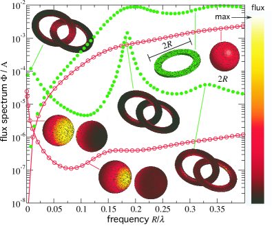
Figure 2: Flux spectra $\Phi$ of isolated and interacting/interlocked spheres/rings (solid/hollow circles) of radii $R=1\mu$m, normalized by their corresponding surface areas $A$, computed via Eq. 2. Solid lines denote $\Phi$ as computed via the semi-analytical formulas of Narayanaswamy and Chen (2008); Golyk et al. (2012). Insets show the spatial distribution of surface flux pattern at particular frequencies (right colorbar).

Results: Figure 1 shows the flux spectrum $\Phi$ for various configurations of gold spheres and cylinders (of radii $R=0.2\mu$m and varying lengths $L$), as a function of frequency $R/\lambda$. ($\Phi$ is normalized by the surface area $A$ of each object to make comparisons easier. At these wavelengths, $R$ is several times the skin depth $\delta=c/\sqrt{\varepsilon}\omega$, which means that most of the radiation is coming from sources near the surface Golyk et al. (2012).) Our results for isolated and interacting spheres (red hollow circles) agree with previous results based on semi-analytical formulas Narayanaswamy and Chen (2008); Golyk et al. (2012) (solid lines). In addition, Fig. 1 shows $\Phi$ for isolated and interacting cylinders (solid circles) of various aspect ratios $L/R$; previous results based on semi-analytical methods (solid lines) were limited to the infinite case $L/R\to\infty$ Golyk et al. (2012). For $L/R\approx 1$ (not shown), corresponding to nearly-isotropic cylinders, $\Phi$ is only slightly larger than that of an isolated sphere due to the small but non-negligible volume contribution to $\Phi$. As $L/R$ increases, $\Phi$ increases over all $\lambda$, and converges towards the $L\to\infty$ limit (black solid line) as $\lambda\to 0$, albeit slowly. Interestingly, $\Phi_{L}\gg\Phi_{\infty}$ at particular wavelengths, a consequence of geometrical resonances that are absent in the infinite case. (Away from these resonances, $\Phi$ clearly straddles the $L\to\infty$ result so long as $\lambda\lesssim L$.) For interacting cylinders, in addition to the expected near-field enhancement at large $\lambda$, one also finds significant resonant peaks at $\lambda\lesssim L$.

Equation 2 can be exploited to obtain $\Phi$ in an even more complicated geometry, where the topology makes it difficult to distinguish the incoming and outgoing waves of other formulations Bimonte (2009); Kruger et al. (2011); Messina and Antezza (2011). Figure 2 shows $\Phi$ for isolated and interlocked gold rings (solid circles), of inner and outer radii $r=0.7\mu$m and $R=1\mu$m, respectively, and thickness $h=0.1\mu$m. For comparison, we also show the corresponding $\Phi$ for isolated and interacting spheres of radii $R$ (open circles). As in the case of finite cylinders, the rings exhibit orders of magnitude enhancement in $\Phi$ at particular $\lambda$, corresponding to azimuthal resonances—the first of which is the $m=0$ mode at $\lambda\approx 2\pi R$. Interestingly, despite its smaller surface area and volume, the absolute (unnormalized) $\Phi$ of the isolated ring is $\approx 4.5$ times larger than that of the sphere at the fundamental resonance. The geometrical origin of this resonance enhancement becomes even more apparent upon inspection of the spatial distribution of flux pattern on the surface of the objects, which we compute via Eq. 7 and show as insets in Fig. 2, for both rings and spheres. As expected, at large wavelengths $\lambda\gg R$, near-field effects dominate and the flux pattern peaks in regions of nearest surfaces. However, for $\lambda\sim R$, the sphere–sphere pattern does not change qualitatively while the ring–ring pattern exhibits resonance patterns characterized by nodes and peaks distributed along the ring. (Interestingly, the flux pattern of the first resonance is peaked away from the nearest surfaces.) Away from these resonances, the ring emissivity is smaller: for $\lambda\ll R$ (not shown), $\Phi$ is well described by the Stephan-Boltzmann law, and the ratio of their emissivities is given by the ratio of their surface areas $\approx 0.3$. A similar reduction occurs for $\lambda\gg R$ due to the ring’s smaller polarizability.

This work was supported by DARPA Contract No. N66001-09-1-2070-DOD and by the AFOSR Multidisciplinary Research Program of the University Research Initiative (MURI) for Complex and Robust On-chip Nanophotonics, Grant No. FA9550-09-1-0704.

References

- Rytov et al. (1989) S. M. Rytov, V. I. Tatarskii, and Y. A. Kravtsov, Principles of Statistical Radiophsics II: Correlation Theory of Random Processes (Springer-Verlag, 1989).
- Polder and Van Hove (1971) D. Polder and M. Van Hove, Phys. Rev. B 4, 3303 (1971).
- Loomis and Maris (1994) J. J. Loomis and H. J. Maris, Phys. Rev. B 50, 18517 (1994). J. B. Pendry, J. Phys: Cond. Matt. 11, 6621 (1999). K. Joulain, J.-P. Mulet, F. Marquier, R. Carminati, and J.-J. Greffet, Surf. Sci. Rep. 57, 59 (2005). V. P. Carey, G. Cheng, C. Grigoropoulos, M. Kaviany, and A. Majumdar, Nanoscale Micro. Thermophys. Eng. 12, 1 (2006).
- Volokitin and Persson (2007) A. Volokitin and B. Persson, Rev. Mod. Phys. 79, 1291 (2007).
- Zhang (2007) Z. M. Zhang, Nano/Microscale Heat Transfer (McGraw-Hill, New York, 2007).
- Basu et al. (2009) S. Basu, Z. M. Zhang, and C. J. Fu, Int. J. Energy Res. 33, 1203 (2009).
- Rousseau et al. (2009) E. Rousseau, A. Siria, J. Guillaume, S. Volz, F. Comin, J. Chevrier, and J.-J. Greffet, Nat. Phot. 3, 514 (2009).
- Shen et al. (2009) S. Shen, A. Narayanaswamy, and G. Chen, Nano Letters 9, 2909 (2009).
- Reid et al. (2012) H. Reid, J. White, and S. G. Johnson, arXiv:1203.0075 (2012).
- Narayanaswamy and Chen (2008) A. Narayanaswamy and G. Chen, Phys. Rev. B 77, 075125 (2008).
- Bimonte (2009) G. Bimonte, Phys. Rev. A 80, 042102 (2009).
- Messina and Antezza (2011) R. Messina and M. Antezza, Phys. Rev. A 84, 042102 (2011).
- Kruger et al. (2011) M. Kruger, T. Emig, and M. Kardar, Phys. Rev. Lett. 106, 210404 (2011).
- Otey and Fan (2011) C. Otey and S. Fan, Phys. Rev. B 84 (2011).
- Guerout et al. (2012) R. Guèrout, J. Lussange, F. S. S. Rosa, J. P. Hugonin, D. A. R. Dalvit, J. J. Greffet, A. Lambrecht, and S. Reynaud, arXiv:1203.1496 (2012).
- Rodriguez et al. (2011) A. W. Rodriguez, O. Ilic, P. Bermel, I. Celanovic, J. D. Joannopoulos, M. Soljacic, and S. G. Johnson, Phys. Rev. Lett. 107, 114302 (2011).
- Rao and Balakrishnan (1999) S. M. Rao and N. Balakrishnan, Curr. Sci. 77, 1343 (1999).
- Eckhardt (1984) W. Eckhardt, Phys. Rev. A 29, 1991 (1984).
- Jackson (1998) J. D. Jackson, Classical Electrodynamics (Wiley, New York, 1998), 3rd ed.
- Chen (1989) K.-M. Chen, IEEE Trans. Microwave Theory Tech. 37, 1576 (1989).
- Golyk et al. (2012) V. A. Golyk, M. Kruger, and M. Kardar, Phys. Rev. E 85, 046603 (2012).