Magnetometry of the classical T Tauri star GQ Lup: non-stationary dynamos & spin evolution of young Suns

Abstract

We report here results of spectropolarimetric observations of the classical T Tauri star (cTTS) GQ Lup carried out with ESPaDOnS at the Canada-France-Hawaii Telescope (CFHT) in the framework of the ‘Magnetic Protostars and Planets’ (MaPP) programme, and obtained at 2 different epochs (2009 July and 2011 June). From these observations, we first infer that GQ Lup has a photospheric temperature of $4,300\pm 50$ K and a rotation period of $8.4\pm 0.3$ d; it implies that it is a $1.05\pm 0.07$ ${\rm M}_{\odot}$ star viewed at an inclination of $\simeq$30^∘, with an age of 2–5 Myr, a radius of $1.7\pm 0.2$ ${\rm R}_{\odot}$, and has just started to develop a radiative core.

Large Zeeman signatures are clearly detected at all times, both in photospheric lines and in accretion-powered emission lines, probing longitudinal fields of up to 6 kG and hence making GQ Lup the cTTS with the strongest large-scale fields known as of today. Rotational modulation of Zeeman signatures, also detected both in photospheric and accretion proxies, is clearly different between our 2 runs; we take this as further evidence that the large-scale fields of cTTSs are evolving with time and thus that they are produced by non-stationary dynamo processes.

Using tomographic imaging, we reconstruct maps of the large-scale field, of the photospheric brightness and of the accretion-powered emission at the surface of GQ Lup at both epochs. We find that the magnetic topology is mostly poloidal and axisymmetric with respect to the rotation axis of the star; moreover, the octupolar component of the large-scale field (of polar strength 2.4 and 1.6 kG in 2009 and 2011 respectively) dominates the dipolar component (of polar strength $\simeq$1 kG) by a factor of $\simeq$2, consistent with the fact that GQ Lup is no longer fully-convective.

GQ Lup also features dominantly poleward magnetospheric accretion at both epochs. The large-scale dipole component of GQ Lup is however not strong enough to disrupt the surrounding accretion disc further than about half-way to the corotation radius (at which the Keplerian period of the disc material equals the stellar rotation period), suggesting that GQ Lup should rapidly spin up like other similar partly-convective cTTSs.

We finally report a 0.4 km s^-1 RV change for GQ Lup between 2009 and 2011, suggesting that a brown dwarf other than GQ Lup B may be orbiting GQ Lup at a distance of only a few au’s.

1 Introduction

It is now well recognised that magnetic fields can significantly modify the life of stars and in particular their rotation rates. Their impact is thought to be strongest throughout the formation stages, when stars and their planetary systems build up from the collapse of giant molecular clouds. More specifically, fields are likely efficient at slowing down the cloud collapse, at inhibiting the subsequent fragmentation and at dissipating the cloud angular momentum through magnetic braking and the associated magnetised outflows / collimated jets (e.g., Donati & Landstreet, 2009; André et al., 2009, for reviews). At a later stage, the newly born protostars (called classical T Tauri stars or cTTSs) are apparently capable of generating magnetic fields strong enough to disrupt the central regions of their accretion discs and to funnel some of the inner disc material onto the stellar surface, thereby drastically modifying the overall mass accretion process (e.g., Bouvier et al., 2007a).

For some time, the strong magnetic fields of cTTSs could only be inferred through indirect proxies such as continuum or line emission throughout the whole electromagnetic spectrum, from X-rays to radio wavelengths. Directly detected for the first time about 2 decades ago through the Zeeman broadening they induce on spectral lines observed in unpolarized light (e.g., Johns-Krull, 2007, for a recent overview), magnetic fields of cTTSs can now be characterized by various means. In particular, their large-scale topologies - controlling how the fields couple the central protostars to the inner regions of their accretion discs and thereby how disc material is being accreted - can be thoroughly investigated thanks to the advent of sensitive high-resolution spectropolarimeters dedicated to the study of stellar magnetic fields (e.g., Donati, 2003; Donati & Landstreet, 2009). By measuring circularly-polarised Zeeman signatures of cTTSs and by monitoring their rotational modulation, one can reconstruct the parent large-scale magnetic topologies, thus offering the possibility of studying magnetospheric accretion processes in a much more quantitative way.

The international MaPP (Magnetic Protostars and Planets) project was designed mostly for this purpose. The first main goal of MaPP is to investigate (through a first survey of $\simeq 15$ targets, with some of them observed at several epochs) how the large-scale magnetic topologies of cTTSs depend on key stellar parameters such as mass, age, rotation and accretion rate (e.g., Donati et al., 2010; Donati et al., 2011b). The second main goal of MaPP is to provide an improved theoretical description, using both analytical modelling and numerical simulations, of how magnetic fields of cTTSs are generated and how they modify mass accretion processes (see, e.g., Gregory et al., 2010; Romanova et al., 2011), and more generally how critically they impact the formation of low-mass stars. A total of 690 hr of time was allocated for MaPP on the 3.6 m Canada-France-Hawaii Telescope (CFHT) over a timescale of 9 semesters (2008b-2012b). Up to now magnetic Zeeman signatures were detected on all selected targets; several major discoveries were achieved regarding the two science goals mentioned above, that we will recall below in the light of the new results presented here.

This new study focusses on the cTTS GQ Lup, whose mass is a fair match to that of the Sun and whose age is typical of cTTSs. Located near Lupus 1, in the Lupus star formation region ($150\pm 10$ pc away from the Earth, Wichmann et al., 1999; Crawford, 2000), GQ Lup recently attracted a lot of attention following the discovery of its low-mass companion (most likely a brown dwarf, with a mass in the range 10–40 ${\rm M}_{\rm Jup}$, McElwain et al., 2007; Lavigne et al., 2009) in the outer regions of its accretion disc (at a distance of $\simeq$0.7^′′ or 100 au, Neuhäuser et al., 2005). Although the nature of this sub-stellar companion is still a matter of speculation, it makes GQ Lup an obvious target of study, to investigate the properties of the central protostar on the one hand (and in particular the star-disc interaction in which the large-scale magnetic field of the protostar plays a crucial role) and to better understand how stellar / planetary systems form. In this respect, efforts at modelling the magnetic field of the protostar and associated activity are worthwhile. The large-scale field is obviously a key parameter to unravel the physics of the star-disc magnetospheric interaction, whereas the potential presence of closer companions (e.g., that could explain the ejection on an outer orbit of the very distant companion detected already) can only be revealed through high-precision radial velocity (RV) measurements when an accurate description of the magnetic activity, and an efficient way of filtering the associated RV jitter, become available.

We start this paper by describing the spectropolarimetric observations of GQ Lup we collected at 2 different epochs and from which Zeeman signatures are clearly detected (Sec. 2). Following a fresh re-determination of the main characteristics of this cTTS (Sec. 3), we outline the rotational modulation and intrinsic long-term variability that we observe in the data (Sec. 4). We then detail the modelling of these data with our magnetic imaging code (Sec. 5), compare our new results with previous ones and outline how they improve our understanding of how magnetic fields impact the formation of Sun-like stars (Sec. 6).

2 Observations

Spectropolarimetric observations of GQ Lup were collected at two different epochs, first from 2009 July 01 to 14, then from 2011 June 08 to 23, using the high-resolution spectropolarimeter ESPaDOnS at the Canada-France-Hawaii Telescope (CFHT). ESPaDOnS collects stellar spectra spanning the entire optical domain (from 370 to 1,000 nm) at a resolving power of 65,000 (i.e., resolved velocity element of 4.6 km s^-1), in either circular or linear polarisation (Donati, 2003). In 2009 (resp. 2011), a total of 14 (resp. 12) circular polarisation spectra were collected over a timespan of 14 (resp. 16) nights with as regular a time sampling as possible (about 1 spectrum per night) given weather conditions. All polarisation spectra consist of 4 individual subexposures (each lasting 904 s and 853.5 s in 2009 and 2011 respectively) taken in different polarimeter configurations to allow the removal of all spurious polarisation signatures at first order. All raw frames are processed as described in the previous papers of the series (e.g., Donati et al., 2010; Donati et al., 2011a), to which the reader is referred for more information. The peak signal-to-noise ratios (S/N, per 2.6 km s^-1 velocity bin) achieved on the collected spectra range between 60 and 250 depending on weather/seeing conditions with a median value of about 200. The full journal of observations is presented in Table 1.

Table 1: Journal of observations collected in 2009 July and 2011 June. Each observation consists of a sequence of 4 subexposures (each lasting 904 s and 853.5 s in 2009 and 2011 respectively). Columns $1-4$ respectively list the UT date, the Heliocentric Julian Date (HJD) and UT time (both at mid-exposure), and the peak signal to noise ratio (per 2.6 km s^-1 velocity bin) of each observation. Column 5 lists the rms noise level (relative to the unpolarized continuum level $I_{\rm c}$ and per 1.8 km s^-1 velocity bin) in the circular polarization profile produced by Least-Squares Deconvolution (LSD), while column 6 indicates the orbital/rotational cycle associated with each exposure (using the ephemeris given by Eq. 1).

Date	HJD	UT	S/N	$\sigma_{\rm LSD}$	Cycle
2009	(2,455,000+)	(h:m:s)		($10^{-4}I_{\rm c}$)	(0+)
Jul 01	13.81216	07:25:13	140	3.3	0.097
Jul 02	14.81245	07:25:45	180	2.4	0.216
Jul 03	15.80196	07:10:45	200	2.2	0.334
Jul 04	16.79606	07:02:22	180	2.5	0.452
Jul 05	17.79593	07:02:17	200	2.2	0.571
Jul 06	18.79716	07:04:11	180	2.4	0.690
Jul 07	19.79736	07:04:34	120	4.1	0.809
Jul 08	20.79778	07:05:18	170	2.7	0.928
Jul 09	21.79511	07:01:34	120	3.9	1.047
Jul 10	22.79485	07:01:18	190	2.3	1.166
Jul 11	23.80029	07:09:15	60	8.8	1.286
Jul 12	24.81958	07:37:09	190	2.4	1.407
Jul 13	25.75895	06:09:58	210	2.1	1.519
Jul 14	26.75935	06:10:39	190	2.5	1.638
Date	HJD	UT	S/N	$\sigma_{\rm LSD}$	Cycle
2011	(2,455,700+)	(h:m:s)		($10^{-4}I_{\rm c}$)	(84+)
Jun 08	20.96469	11:02:45	140	3.3	0.281
Jun 11	23.91064	09:45:08	240	1.7	0.632
Jun 12	24.93835	10:25:06	240	1.8	0.755
Jun 14	26.86920	08:45:42	180	2.5	0.984
Jun 15	27.88564	09:09:27	240	1.8	1.105
Jun 16	28.88107	09:02:57	190	2.3	1.224
Jun 17	29.84680	08:13:41	190	2.2	1.339
Jun 18	30.91269	09:48:40	220	2.0	1.466
Jun 20	32.91118	09:46:40	250	1.8	1.704
Jun 21	33.84406	08:10:07	250	1.8	1.815
Jun 22	34.93027	10:14:21	240	1.9	1.944
Jun 23	35.91838	09:57:20	210	2.2	2.062

As outlined in Sec. 4, we find that the rotation period of GQ Lup is $8.4\pm 0.3$ d, i.e., very similar to that derived by Broeg et al. (2007). Rotational cycles $E$ of GQ Lup are thus computed from Heliocentric Julian Dates (HJDs) according to the following ephemeris:

$$\mbox{HJD}=2455013.0+8.4E.$$ (1)

Coverage of the rotation cycle is reasonably dense and regular in 2009 and 2011, at which $\simeq$1.6 and 2 complete cycles of GQ Lup were monitored, offering us a convenient way of disentangling intrinsic variability from rotational modulation in the spectra (see Sec. 4).

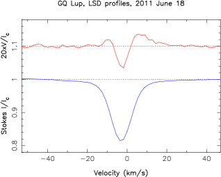
Figure 1: LSD circularly-polarized (Stokes $V$) and unpolarized (Stokes $I$) profiles of GQ Lup (top/red, bottom/blue curves respectively) collected on 2011 June 18 (cycle 84+1.466). A clear Zeeman signature (with a full amplitude of 0.5% and featuring a double sign switch across the line) is detected in the LSD Stokes $V$ profile, in conjunction with the unpolarised line profile. The mean polarization profile is expanded by a factor of 20 and shifted upwards by 1.1 for display purposes.

Least-Squares Deconvolution (LSD, Donati et al., 1997) was applied to all observations. The line list we employed for LSD is computed from an Atlas9 LTE model atmosphere (Kurucz, 1993) and corresponds to a K6IV spectral type ($\hbox{$T_{\rm eff}$}=4,250$ K and $\hbox{$\log g$}=4.0$) appropriate for GQ Lup. As usual, only moderate to strong atomic spectral lines are included in this list (see, e.g., Donati et al., 2010, for more details). Altogether, about 8,900 spectral features (with about 40% from Fe i) are used in this process. Expressed in units of the unpolarized continuum level $I_{\rm c}$, the average noise levels of the resulting Stokes $V$ LSD signatures range from 1.7 to 8.8$\times 10^{-4}$ per 1.8 km s^-1 velocity bin (median value 2.3$\times 10^{-4}$). Zeeman signatures are detected at all times in LSD profiles and in most accretion proxies (see Sec. 4); an example LSD photospheric Zeeman signature (collected during the 2011 run) is shown in Fig. 1 as an illustration.

3 GQ Lup

Some of the important characteristics of GQ Lup are not presently known with good accuracy; in particular, the photospheric temperature $T_{\rm eff}$, usually taken as 4060 K and derived from the spectral type (i.e., K7eV Neuhäuser et al., 2005), is only a crude approximation (not accurate to better than 250 K). Given that the estimated mass of cTTSs like GQ Lup (usually in the approximately isothermal Hayashi phase of their contraction, where they follow roughly vertical tracks downwards in the Hertzsprung-Russel diagram, towards the main sequence) mostly depends on the photospheric temperature, deriving as accurate an estimate of $T_{\rm eff}$ as possible is of obvious concern for our study, especially when it comes to investigating how the magnetic topology relates to the internal structure of the protostar (see Sec. 6).

Towards this aim, we developed an automatic spectral classification tool similar to previously published ones (e.g., Valenti & Fischer, 2005) and using multiple spectral windows in the wavelength ranges 515–520 nm and 600-620 nm. As a first step, we adjust the parameters of most atomic lines in the domain to match synthetic spectra with those of a handful of standard stars (including the Sun) with $T_{\rm eff}$, logarithmic gravity ($\log g$, with $g$ in cgs units) and logarithmic metallicity (with respect to that of the Sun) in the range 4000 to 6500 K, 3.5 to 4.5 and –0.5 to 0.5; in a second step, we build a library of synthetic spectra for all values of $T_{\rm eff}$, $\log g$ and logarithmic metallicity in the same range, with respective steps of 50 K, 0.1 and 0.1; the final step consists in fitting the observed spectrum to be characterised with all synthetic spectra within the grid, and deriving the stellar parameters that minimise $\chi^{2}$ and the corresponding error bars (from the curvature of the 3D $\chi^{2}$ landscape at the derived minimum); estimates of the radial velocity $v_{\rm rad}$ and of the line-of-sight projected rotation velocity $v\sin i$ are also derived as a by-product, assuming a given microturbulent velocity (set to 1 km s^-1) and a tabulated macroturbulent velocity depending on $T_{\rm eff}$ and $\log g$ (following Valenti & Fischer, 2005). Though still in a preliminary stage, our automatic spectral classification tools (called MagIcS) is found to behave well on standard stars, yielding stellar parameters in agreement with published values within better than 50 K, 0.1 and 0.1 for $T_{\rm eff}$, $\log g$ and logarithmic metallicity. A more detailed description of this tool will be presented in a dedicated paper.

This tool was slightly modified in the specific case of cTTSs, for which optical veiling (i.e., the apparent weakening of the photospheric spectrum, presumably caused by accretion) comes as an additional parameter and makes it fairly difficult to estimate metallicity with reasonable accuracy at the same time. For this purpose, we decided to carry out the fit assuming solar metallicity (for the grid of synthetic spectra); we otherwise proceed in exactly the same way for deriving $T_{\rm eff}$ and $\log g$ (with their error bars, along with $v\sin i$, $v_{\rm rad}$ and veiling). When tested on standard cTTSs like BP Tau, AA Tau or V2129 Oph, MagIcS is found again to provide $T_{\rm eff}$ and $\log g$ compatible with published values within better than 50 K and 0.2; applying it to GQ Lup, we obtain $\hbox{$T_{\rm eff}$}=4,300$ K and $\hbox{$\log g$}=3.7$. In particular, the photospheric temperature we derive is significantly larger than the estimate quoted in most studies (4060 K); it is closer to the estimate derived from multi-colour photometry by McElwain et al. (2007), equal to $\simeq$4200 K. We believe that our new measurement, based on high-S/N high-resolution spectra (see Sec. 2) and obtained through a direct comparison (calibrated on standard stars) of observed and synthetic spectral lines, is more accurate than the two quoted published values (estimated either from the spectral type or from spectrophotometry only) and hence use it in the following.

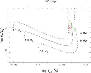
Figure 2: Observed (open square and error bars) location of GQ Lup in the HR diagram. The PMS evolutionary tracks and corresponding isochrones (Siess et al., 2000) assume solar metallicity and include convective overshooting. The green line depicts where models predict cTTSs start developing their radiative core as they contract towards the main sequence.

The revised mass of GQ Lup that we derive (mostly from $T_{\rm eff}$ and a comparison with evolutionary models of Siess et al., 2000, see Fig. 2) is $1.05\pm 0.07$ ${\rm M}_{\odot}$ (the error bar reflecting mainly the uncertainty on $T_{\rm eff}$). This is significantly larger than most estimates published so far (usually in the range 0.7–0.8 ${\rm M}_{\odot}$, e.g., Neuhäuser et al., 2005; Seperuelo Duarte et al., 2008, essentially reflecting the difference in $T_{\rm eff}$) but more in line with the findings of McElwain et al. (2007, also favouring a larger $T_{\rm eff}$). In addition to small ($<$0.5 mag) photometric fluctuations attributed as usual to the presence of cool spots coming and going on the visible hemisphere of the protostar (e.g., Broeg et al., 2007), GQ Lup is also reported to undergo much larger dimming episodes (of up to 2 mag, e.g., Covino et al., 1992) that can hardly be caused by cool starspots but more likely by extinction (e.g., by circumstellar material passing onto the line of sight); by considering only epochs at which the photometric brightness is highest and the photometric variability is smallest (as in, e.g., Janson et al., 2006), one can derive an estimate of the unspotted, unextincted, $V$ brightness of GQ Lup, equal to $V=11.4\pm 0.2$ (e.g., Broeg et al., 2007). Using the above mentioned distance ($150\pm 10$ pc) as well as the bolometric correction corresponding to our temperature estimate ($-0.74\pm 0.05$, e.g., Bessell et al., 1998), we finally obtain that GQ Lup has a bolometric magnitude of $4.78\pm 0.25$ (corresponding to a logarithmic luminosity with respect to the Sun of $\log\hbox{$L_{\star}$}/\hbox{${\rm L}_{\odot}$}=0.0\pm 0.1$, see Fig. 2) and thus a radius of $1.7\pm 0.2$ ${\rm R}_{\odot}$ (in reasonable agreement with the findings of Seperuelo Duarte et al., 2008, despite the different values of $T_{\rm eff}$ used in both studies). The (conservative) error bar on the radius mostly reflects those on the luminosity and temperature. By comparing to evolutionary models of Siess et al. (2000, see Fig. 2), we find that GQ Lup has an age of 2–5 Myr, in good agreement with the estimates of McElwain et al. (2007) and Seperuelo Duarte et al. (2008); evolutionary models also predict that, at this age, GQ Lup should no longer be fully-convective and should host a radiative core extending up to $\simeq$0.25 $R_{\star}$ in radius (Siess et al., 2000).

4 Spectroscopic variability

Before carrying out a full modelling of our spectropolarimetric data (see Sec. 5), we first present a simple phenomenological description of how the photospheric LSD profile and the selected accretion proxies (i.e., Ca ii IRT, He i $D_{3}$, H${\alpha}$ and H${\beta}$) vary with time over each of our 2 observing runs. More specifically, this first step consists in looking at how equivalent widths, RVs and longitudinal magnetic fields (i.e., the line-of-sight projected component of the vector field averaged over the visible stellar hemisphere and weighted by brightness inhomogeneities) are modulated by rotation, in order to derive a rough, mostly intuitive, idea about the nature and orientation of the large-scale field of GQ Lup, and about the surface distribution of cool photospheric spots and hot chromospheric accretion regions.

4.1 The rotation period

A recent search for photometric (and RV) modulation by Broeg et al. (2007) has suggested that the rotation period of GQ Lup is $8.45\pm 0.2$ d, typical of that of cTTSs in the mass range 0.5–1.2 ${\rm M}_{\odot}$ and with ages of $<$5 Myr. Clear modulation at this period is found in their data (at 2 different epochs), as well as in several (though not all) older photometric light curves published in the literature over the last 2 decades; this modulation is potentially also present in the RV estimates derived with cross-correlation from a series of high-resolution spectra. Modulation of the amount of veiling in the spectrum of GQ Lup is also reported by Seperuelo Duarte et al. (2008) from spectrophotometric observations covering a timespan of 17 d; the period they report is however significantly longer, equal to 10.7 d, compatible with the one they determine from archival B band photometry ($10.43\pm 0.12$ d). This apparent discrepancy may be caused by intrinsic variability (rendering rotation period of cTTSs difficult to estimate precisely) or reflect something real, such as differential rotation, at the surface of GQ Lup. As detailed in the following subsections, our own data (and in particular the 2009 data set) also show clear rotational modulation, both in the circularly polarized and the unpolarized profiles of photospheric lines and accretion proxies) at an average period of $8.4\pm 0.3$ d. We therefore selected this period as the main rotation period of GQ Lup, and used it to phase all our data (see Sec. 2).

Given the $v\sin i$ we estimate (equal to $5\pm 1$ km s^-1, see Sec. 5), we derive (from the radius and rotation period) that the rotation axis of GQ Lup is inclined at $\simeq$30^∘ to the line of sight, and hence that GQ Lup is seen mostly pole-on (rather than equator on), in agreement with the findings of Broeg et al. (2007) and with a recent estimate of the viewing angle of the accretion disc from interferometric data (Anthonioz, private communication).

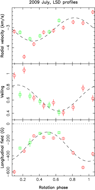
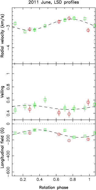
Figure 3: Rotational modulation of the RV (top row), veiling (second row) and longitudinal field (bottom row) derived from the LSD photospheric profiles of GQ Lup in 2009 July (left panels) and in 2011 June (right panels). Data collected during the first and second rotational cycles of each run (i.e., corresponding to phases 0.07–1.07 and 1.07–2.07 respectively) are shown with red circles and green squares. Formal $\pm$1 $\sigma$ error bars (computed from the error bars of the observed spectra) are shown for longitudinal fields, while conservative error bars of $\pm$0.1 km s^-1 and $\pm$0.05 were assumed for RVs and veiling respectively. Fits with sine/cosine waves are included (and shown as dashed lines) to outline (whenever significant) the amount of variability attributable to rotational modulation.

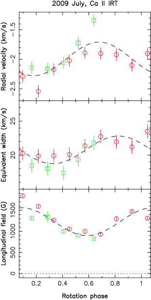
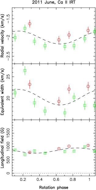
Figure 4: RVs (top row), equivalent widths (second row) and longitudinal fields (bottom row) derived from the Ca ii IRT LSD profiles of GQ Lup in 2009 July (left panels) and in 2011 June (right panels), with symbol/color coding as in Fig. 3. Conservative error bars of $\pm$0.1 and $\pm$1 km s^-1 were assumed for the RVs and equivalent widths of the emission profile.

4.2 LSD photospheric profiles

We first examine the temporal variability of unpolarized and circularly polarized LSD profiles of GQ Lup, summarised graphically in Fig. 3 for both observing epochs. In 2009 July (left column of Fig. 3), RVs of Stokes $I$ LSD profiles show clear and smooth rotational modulation about a mean RV of $\hbox{$v_{\rm rad}$}=-3.2\pm 0.1$ km s^-1 and with a full amplitude of $\simeq$1.2 km s^-1 that repeats quite well between the 2 observed cycles, except for 2 stray points at rotation cycles 0.216 and 1.047 that are typically off by $\simeq$1 km s^-1 from the average trend. In 2011 June (right column of Fig. 3), Stokes $I$ LSD profiles are on average slightly (but significantly) red-shifted with respect to those of 2009 July ($\hbox{$v_{\rm rad}$}=-2.8\pm 0.1$ km s^-1) and exhibit a smaller level of rotational modulation (full RV amplitude of $\simeq$0.5 km s^-1), but are otherwise very similar and repeat in particular rather well between the 2 observed cycles. It is reasonable to assume that the rotational modulation we detect is mostly caused by the presence of cool spots at the surface of GQ Lup, as for all other cTTSs already studied in our sample (e.g., Donati et al., 2011a). The small amplitude of the RV rotational modulation (relative to the line-of-sight projected rotational velocity, $\hbox{$v\sin i$}\simeq 5$ km s^-1) suggests that the main cool spot causing the RV changes is located at high-latitudes (as for most other cTTSs), and even more so in 2011 June than in 2009 July; moreover, the parent spot is presumably centred around phase 0.0–0.1 (i.e., at mid-phase between RV maximum and minimum). The period on which RVs fluctuate is found to be equal to $8.8\pm 0.6$ d and $9.2\pm 0.6$ d in 2009 July and 2011 June respectively, i.e., marginally longer than (though still compatible with) the assumed rotation period on which all data were phased (equal to 8.4 d, see Eq. 1). The clear change in the RV curve between the 2 epochs demonstrates that the spot configuration significantly evolved between the 2 epochs, as opposed to what is seen on TW Hya (where the high-latitude spot configuration remained more or less stable for the last 3 yrs, Donati et al., 2011b). The origin of the small shift in $v_{\rm rad}$ (about $-0.4$ km s^-1 between 2009 and 2011) is unclear, and unlikely attributable to the distant brown dwarf companion previously reported GQ Lup B (too distant to generate such a change in as little as 2 yr).

The spectrum of GQ Lup is also significantly veiled at both our observing epochs, with average veiling (at about 640 nm, the average wavelength of LSD profiles) varying from 0.4 to 1 (see middle panels of Fig. 3). Veiling variations are weak in 2011 June ($\simeq$10% peak to peak about an average veiling of $\simeq$0.5) but significantly stronger in 2009 July where veiling is clearly modulated by rotation (by $\simeq$40% peak to peak, about a mean of $\simeq$0.65 and with a period of $8.2\pm 0.6$ d), suggesting that GQ Lup was in a more active state of accretion in 2009 July than in 2011 June. In 2009 July, veiling is found to peak around phase 0.1, i.e., when the cool polar spot detected at the surface of GQ Lup (through RV changes) comes closest to the observer. This suggests that the hot chromospheric spot presumably causing the veiling variations roughly overlaps the cool photospheric spot, e.g., as in most other cTTSs we studied to date.

Zeeman signatures of GQ Lup are detected at all times, showing in most cases a canonical shape (i.e., antisymmetric with respect to the line centre) with a peak-to-peak amplitude ranging from 0.3 to 1.1%, except at a few rotational cycles (e.g., cycle 84+1.466, see Fig. 1) where the Zeeman signature exhibits a more complex shape (e.g., featuring a double sign switch across the line profile). The corresponding longitudinal field is found to be negative at all times, ranging from –75 to –600 G (with typical error bars of 10–20 G). As for RVs, longitudinal fields show clear rotational modulation (see bottom panels of Fig. 3), especially in 2009 July where the peak-to-peak fluctuation reaches almost 400 G with a well defined period of $8.4\pm 0.3$ d (the period that we selected for phasing all our data, see Eq. 1). The longitudinal field of GQ Lup is found to reach maximum strength around phase 0.9-1.0, i.e. slightly leading the high-latitude cool spot tracked through RV changes (best viewed at phase $\simeq$0.1). The drastic change in the amplitude of the longitudinal field curve between 2009 and 2011 also indicates that the large-scale field of GQ Lup has significantly evolved between our two observing epochs. In addition to rotational modulation (dominant in 2009), intrinsic variability is also clearly detected at both epochs and likely reflects local, rapid changes at the surface of GQ Lup (e.g., in the photospheric brightness distribution) possibly resulting from unsteady accretion.

4.3 Ca ii IRT emission

We use core emission in the Ca ii IRT lines as our main proxy of surface accretion; despite the inconvenience of including a dominant contribution from the non-accreting chromosphere, this proxy demonstrates a number of clear advantages over the more conventional He i $D_{3}$ accretion proxy. In particular, Ca ii IRT lines are formed closer to the stellar surface and in a more static atmosphere, making them easier (and less-model dependent) to interpret in terms of large-scale magnetic topologies, with no need to model the velocity flow in the line formation region; they also provide higher quality data which usually overcompensates the signal dilution from the non-accreting chromospheric regions. We start by building up a Ca ii IRT emission profile for each of our spectra; we achieve this by constructing LSD-like weighted averages of the 3 IRT lines, then by subtracting the underlying (much wider) Lorentzian absorption profiles, with a single Lorentzian fit to the far line wings (see Donati et al., 2011b, for an illustration). As for photospheric LSD profiles, we finally examine how the RVs, equivalent widths and longitudinal fields of these emission profiles vary with time throughout our 2 observing runs; these variations are graphically summarised in Fig. 4.

We first note that Ca ii emission strengths are roughly equal at both epochs, with average equivalent widths of $\simeq$21 km s^-1 (or 0.060 nm, see middle panels of Fig. 4). Rotational modulation is only moderate (smaller than 25% peak-to-peak) but clear in 2009 July (where the modulation period is found to be $8.9\pm 0.7$ d, larger though still compatible with that assumed in Eq. 1), while intrinsic variability can be significant at times (e.g., 2011 June). Moreover, Ca ii emission profiles exhibit regular RV fluctuations about a mean of $-2.0\pm 0.1$ km s^-1 in 2009 July and $-1.9\pm 0.1$ in 2011 June, i.e., red-shifted by typically $0.9-1.2$ km s^-1 with respect to the photospheric spectrum (as observed so far for moderately accreting cTTSs, see, e.g., Donati et al., 2011b, and references therein). The full amplitude of the RV rotational modulation is small (with respect to the rotational line broadening), of order 0.5 km s^-1 at both epochs, suggesting that the region of excess Ca ii emission causing this modulation is located at high-latitudes; the period of the RV modulation is found to be $8.1\pm 0.5$ and $8.3\pm 0.9$ d in 2009 July and 2011 June respectively, in agreement with the rotation period used to phase our data.

In 2011 June (right column of Fig. 4), we note that Ca ii emission RV variations are mostly anti-correlated with those of LSD profiles, as often the case for moderately accreting cTTSs (e.g., TW Hya, Donati et al., 2011b) and naturally expected when chromospheric regions of Ca ii excess emission are roughly co-spatial with cool photospheric spots. Whereas this modulation suggests that the parent accretion region is centred at phase $\simeq$0.9 (i.e., midway between RV minimum and maximum), Ca ii excess emission is found to reach maximum around phase 0.15 (though with a high-level of intrinsic dispersion, see Fig. 4, right column, second graph); this is roughly compatible with the position of the photospheric cool spot as derived from LSD photospheric profiles (around phase 0.0–0.1), phase delays as large as 0.1 rotation cycle being much easier to produce (and therefore not necessarily very significant) at high latitudes (where they correspond to shorter physical distances) than at low latitudes.

The situation is less clear in 2009 July. Whereas Ca ii emission strength peaks around phase 0.85, the corresponding RVs suggest that the accretion spot is located around phase 0.45 (i.e. half way between phases of RV minimum and maximum); in particular, RVs of Ca ii emission are largely correlated (in fact, shifted by $\simeq$0.15 rotation cycle) with those of LSD profiles, rather than being anti-correlated as in most other cases (e.g., on GQ Lup in 2011 June). At this point, we have no clear idea as to why RVs of Ca ii emission behave in this unusual way at this specific epoch; this is the first such example that we have encountered among the $\simeq$5 cTTSs studied in detail so far. While we need to gather more similar observations to progress on this issue, we recall for now that the observed RV variations, although weird, are low in amplitude (0.5 km s^-1 peak to peak), thus confirming at the very least that the corresponding feature is located close to the pole.

As for LSD profiles, large Zeeman signatures are detected at all times within the emission component of Ca ii IRT lines, with peak-to-peak relative amplitudes of up to 25% in 2009 July. The corresponding longitudinal fields, ranging from 0.8 to 1.9 kG with median error bars of about 35 G (see lower panels of Fig. 4), are the strongest among all cTTSs investigated up to now. Rotational modulation is clear and well sampled in 2009 July (with an average full amplitude of $\simeq$700 G, and a modulation period of $8.0\pm 0.4$ d) but much weaker in 2011 June (full amplitude lower than 200 G) where the longitudinal field hardly exceeds 1 kG; longitudinal field maximum is reached at phase 0.1 in 2009 July and $\simeq$0.9 in 2011 June, confirming that the cool photospheric spot and the chromospheric accretion region (also located at about the same phase given the above mentioned proxies) are roughly cospatial with the main magnetic poles as in most cTTSs analysed up to now. Although present at both epochs, intrinsic variability of longitudinal fields is only moderate on GQ Lup.

As for several other cTTSs, we note the striking difference in magnetic polarity between the (constantly positive) longitudinal fields measured from the Ca ii emission lines and those (always negative) derived from the LSD profiles, which again demonstrates that LSD profiles and IRT lines probe different areas (of different magnetic polarities) over the stellar surface; following previous papers (e.g., Donati et al., 2011a), we suggest that this is once more evidence that the field of GQ Lup is mostly octupolar, with Ca ii IRT lines (and other accretion proxies) probing mostly the high-latitude (positive) magnetic pole and photospheric LSD profiles reflecting essentially the low-latitude belt of (negative) radial field. The strong weakening from 2009 to 2011 of both the average longitudinal field and of the amount of rotational modulation (also detected on LSD photospheric Zeeman signatures) further confirms that the large-scale field has evolved between our 2 observing epochs.

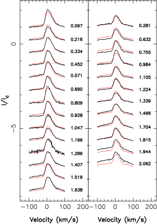
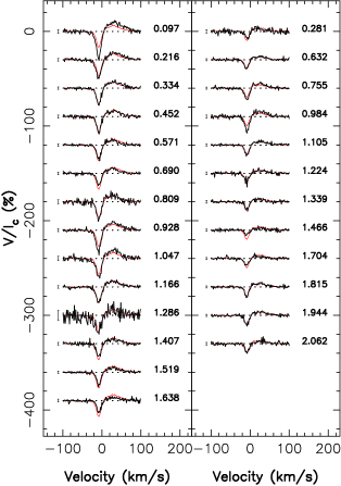
Figure 5: Variations of the unpolarized (Stokes $I$, left panel) and circularly-polarized (Stokes $V$, right panel) profiles of the He i $D_{3}$ emission of GQ Lup in 2009 July (left columns of both panels) 2011 June (right columns). Large Zeeman signatures (with full amplitudes of up to 40% in 2009 July) are clearly detected at all epochs and exhibit shapes that strongly depart from the usual antisymmetric pattern, with a strong / narrow blue (negative) lobe and a weak / wide red (positive) lobe. To emphasize variability, the average profile over each run is shown in red. Rotation cycles (as listed in Table 1) and 3$\sigma$ error bars (for Stokes $V$ profiles only) are shown next to each profile.

4.4 He i $D_{3}$ emission

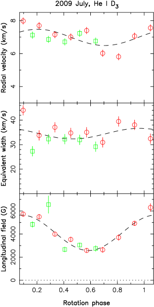
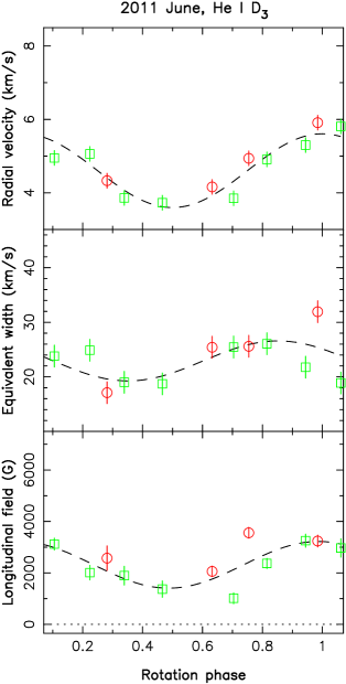
Figure 6: Same as Fig. 4 for the narrow component of the He i $D_{3}$ profiles of GQ Lup. Conservative error bars of $\pm$0.2 km s^-1 and $\pm$2 km s^-1 were assumed on the RVs and equivalent widths of the emission profile.

During our 2 observing runs, the He i $D_{3}$ line of GQ Lup (see Fig. 5) showed up most of the time as a narrow emission profile (with a typical full width at half maximum of $\simeq$40  km s^-1), sometimes on top of a much broader emission profile (e.g., on rotational cycles 1.944 and 2.062) as for TW Hya (Donati et al., 2011b); here we only consider the narrow emission, presumably probing the postshock zone of the accretion region where the plasma is experiencing a strongly decelerating fall towards the stellar surface. We find that this narrow emission is centred on $\simeq$7 km s^-1 in 2009 July and on $\simeq$4.5 km s^-1, i.e., shifted with respect to the photospheric lines by 7-10 km s^-1 depending on the epoch (making GQ Lup similar to other cTTSs in this respect).

The RV and equivalent width variations of the He i $D_{3}$ emission profile are both compatible with (and thus attributable to) the presence of a hot accretion spot best visible at phases 1.0 and 0.8 for epochs 2009 July and 2011 June respectively (i.e., at maximum equivalent width, and midway between RV minimum and maximum, see Fig. 6, top and middle panels); this is in rough agreement with previous conclusions from both LSD photospheric and Ca ii IRT emission profiles. Since the amplitude of the RV variations are small ($<2$ km s^-1 at both epochs), it again suggests that this accretion spot is located close to the pole. The modulation periods of emission strengths are found to be marginally shorter (i.e., $7.3\pm 1.2$ and $7.6\pm 0.5$ d in 2009 July and 2011 June respectively) than the assumed rotation period, whereas those from RVs are found to be somewhat longer (i.e., $8.8\pm 1.3$ and $9.0\pm 0.3$ d).

We note that the He i emission strength decreased significantly between 2009 July and 2011 June (from 35 to 25 km s^-1, or equivalently from 0.070 to 0.050 nm, see Fig. 6), in agreement with the veiling of photospheric lines (also stronger in 2009 June, see Fig. 3). However, no such decrease is seen in the emission core of the Ca ii line, whose strength is roughly the same at both epochs. Since only a small fraction ($\simeq$25%, see Sec. 5) of the Ca ii emission flux is attributable to accretion, we suspect that the change observed in He i emission and veiling is likely occurring as well in the flux of the Ca ii emission core, but at a low enough level ($\simeq$10% of the overall Ca ii emission flux, if the fraction attributable to accretion varied in the same proportion as the He i emission flux) to remain hidden by, e.g., epoch-to-epoch fluctuations in the (dominant) remaining fraction of the emission flux due to chromospheric activity.

Large Zeeman signatures (with full amplitudes of up to $\simeq$40%) are observed in conjunction with the narrow emission component (see Fig. 5, right panel), probing longitudinal fields ranging from 1 to more than 6 kG (see Fig. 6, lower panels) making GQ Lup the cTTSs with strongest magnetic fields known to date. As observed so far in cTTSs, the shape of He i Zeeman signatures (whenever detected) strongly departs from the usual antisymmetric pattern (with respect to the line centre, see Fig. 5) confirming that the line forms in a region where the accreted plasma is rapidly decelerating.

Rotational modulation and polarity of longitudinal fields are very similar to those of the Ca ii line, demonstrating that both lines are reliable probes of magnetic fields in the accretion region. Intrinsic variability in longitudinal fields (on timescales of days) is larger than formal error bars but nevertheless moderate at both epochs (and in particular lower than the amount of rotational modulation), as already noticed on photospheric LSD profiles and Ca ii emission lines. The clear weakening of the longitudinal field between 2009 July and 2011 June further demonstrates that the large-scale magnetic topology is subject to very significant intrinsic variability on timescales as short as 2 yr. The longitudinal field modulation periods are found to be $7.9\pm 0.3$ and $10.1\pm 0.5$ d in 2009 July and 2011 June respectively. We do not think that differential rotation is likely to explain such variations, since He i emission is obviously coming from near the pole at both epochs, i.e., from regions too close in latitude to generate the observed change in modulation period; we rather suspect intrinsic variability (coupled to a reduced modulation amplitude and a limited coverage) to be causing the unusually large (i.e., 3.4$\sigma$) discrepancy between the estimated modulation period in 2011 and the average period of 8.4 d (taken as the rotation period).

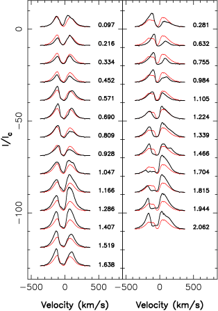
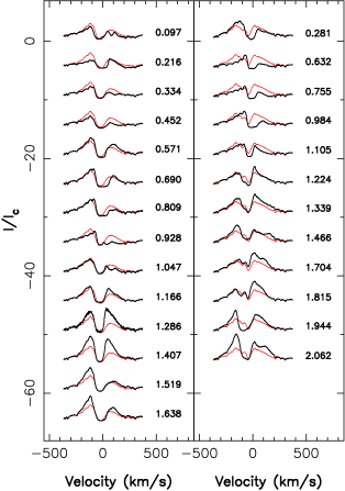
Figure 7: Variations of the H${\alpha}$ (left) and H${\beta}$ (right) lines in the spectrum of GQ Lup, in 2009 July (left column of both panels) and 2011 June (right column). To emphasize variability, the average profile over each run is shown in red. Rotation cycles (as listed in Table 1) are mentioned next to each profile.

4.5 Balmer emission

Unsurprisingly, Balmer lines of GQ Lup are in emission (see Fig. 7), with H${\alpha}$ and H${\beta}$ both showing conspicuous double-peak profiles reminiscent of those of AA Tau (e.g., Bouvier et al., 2007b; Donati et al., 2010); these profiles are in particular more complex than the inverse P Cygni profiles previously reported for GQ Lup from low-resolution spectrophotometric observations (Batalha et al., 2001), in agreement with more recent (also low-resolution spectrophotometric) observations (Seperuelo Duarte et al., 2008). Their respective average equivalent widths are equal to 1,500 & 250 km s^-1 (3.3 & 0.40 nm) in 2009 July and to 1,600 km s^-1 & 400 km s^-1 (3.5 & 0.65 nm) in 2011 June; as a result of the central (blue-shifted) absorption, likely due to winds rather than to accretion (e.g., Seperuelo Duarte et al., 2008), we suspect that these fluxes are lower limits only, rather than true fluxes.

Both lines exhibit strong fluctuations with time, both in their equivalent widths and shape (see Fig. 7). However, these variations do not really correlate well with rotation phase and are thus unlikely attributable to rotational modulation; for instance, the clear strengthening of the red emission peak observed at rotational cycles 1.166–1.407 (in 2009 July) and 1.704–2.0662 (in 2011 June) are not observed one cycle before at both epochs. Note that Balmer line emission is stronger in 2011 than in 2009, and thus does not scale up with the amount of accretion, presumably strongest in 2009 (according to veiling and He i emission fluxes).

The only clear temporal behaviour we can report on Balmer lines (from analyses of autocorrelation matrices) is that the blue wing of the central (blue-shifted) absorption strongly correlates (in both H${\alpha}$ and H${\beta}$) with the overall profile emission strength in 2011 June, this blue wing being strongly blue-shifted (with respect to the average profile) when the emission strength is stronger (e.g., at rotational cycles 84+1.704–2.0662). This may suggest that winds from GQ Lup (presumably causing the central absorption) are also getting faster when they get stronger.

No true absorption is found to occur in the red wing of Balmer lines, and H${\beta}$ in particular, like those found for AA Tau (Bouvier et al., 2007b; Donati et al., 2010) and for V2129 Oph (Donati et al., 2011a; Alencar et al., 2012). As a consequence, no unambiguous constraint can be derived from Balmer lines on the phases at which accretion funnels cross the line of sight (as for both AA Tau and V2129 Oph); this is not really surprising though, given the fact that GQ Lup is viewed mostly pole-on rather than equator-on (see Sec. 3), this viewing configuration being obviously less favourable for detecting the AA Tau-like red-shifted absorption events in Balmer lines thought to be probing episodic crossings of accretion funnels.

4.6 Mass-accretion rate

From the average equivalents widths of the Ca ii IRT, He i and H${\beta}$ lines of GQ Lup, and approximating the stellar continuum by a Planck function at a temperature of 4,300 K (see Sec. 3), we can derive logarithmic line fluxes (with respect to the luminosity of the Sun ${\rm L}_{\odot}$), respectively equal to $-4.8$, $-4.8$ and $-3.9$. This implies logarithmic accretion luminosities (with respect to ${\rm L}_{\odot}$) respectively equal to $-2.0$, $-1.6$ and $-2.0$ (using empirical correlations from Fang et al., 2009). We thus conclude that the average logarithmic mass accretion rate of GQ Lup (in ${\rm M}_{\odot}$ yr^-1) is equal to $-9.0\pm 0.3$, the difference in accretion rates between our 2 observing epochs ($\simeq$0.2 dex) being smaller than the quoted error bar.

Mass accretion rates can in principle also be estimated (though less accurately) through the full width of H$\alpha$ at 10% height (e.g., Natta et al., 2004; Cieza et al., 2010). In the case of GQ Lup, H${\alpha}$ shows a double-peak profile with a full width at 10% height of $500\pm 20$ km s^-1 on average; the logarithmic mass accretion rate estimated from the above mentioned correlation is $-8.0\pm 0.6$ (in ${\rm M}_{\odot}$ yr^-1), only marginally consistent with the above estimate. The origin of this apparent discrepancy (not seen for other similar cTTSs, e.g., Curran et al., 2011) is not clear yet, but could relate to the unusual shape of Balmer lines of GQ Lup (and to their central absorption in particular, possibly leading to an overestimate of the profiles full width at 10% height).

5 Magnetic modelling

In this second phase of the analysis, we aim at converting our sets of photospheric LSD and Ca ii IRT emission profiles into maps of the large-scale magnetic topology, as well as distributions of surface cool spots and of chromospheric accretion regions, at the surface of GQ Lup; for this, we use automatic tools to ensure that our final conclusions are not biased by any preconceived ideas and to independently confirm the preliminary conclusions of Sec. 4. More specifically, we apply to our 2 data sets our now-well-tested tomographic imaging technique, described extensively in previous similar studies (e.g., Donati et al., 2010; Donati et al., 2011a).

Our basic assumption is that the observed profile variations are mainly due to rotational modulation. We thus attempt, following the principles of maximum entropy, at simultaneously and automatically recovering the simplest magnetic topology, photospheric brightness image and accretion-powered Ca ii emission map that are compatible with the series of observed Stokes $I$ and $V$ LSD and Ca ii IRT profiles. For a full description of the imaging method, the reader is referred to the previous papers in the series (e.g., Donati et al., 2010; Donati et al., 2011a).

     

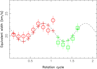
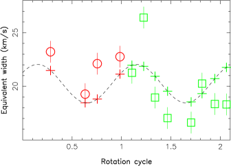
Figure 8: Measured (open symbols) and fitted (pluses) equivalent widths of the Ca ii IRT LSD profiles of GQ Lup in 2009 July (left panel) and 2011 June (right panel). The model wave (dashed line) providing the best (sine+cosine) fit to the data presumably traces rotational modulation (with a period of 8.4 d), while the deviation from the fit illustrates the level of intrinsic variability (significantly higher in 2011 June). The open symbols are defined as described in Fig. 3.

5.1 Application to GQ Lup

We start by applying to the data the usual filtering procedure (e.g., Donati et al., 2010; Donati et al., 2011a), whose aim is to retain the rotational modulation only and hence help the convergence of the imaging code. The effect of this filtering on the Ca ii emission flux is shown for instance in Fig. 8. We stress that this filtering has little impact on the reconstructed images, results derived from the unfiltered data set being virtually identical to those presented below.

We use Unno-Rachkovsky’s equations known to provide a good description of the local Stokes $I$ and $V$ profiles (including magneto-optical effects) in the presence of both weak and strong magnetic fields (e.g., Landi degl’Innocenti & Landolfi, 2004, Sec. 9.8). The model parameters used for GQ Lup are mostly identical to those used in our previous studies (Donati et al., 2010; Donati et al., 2011a); more specifically, the wavelength, Doppler width, unveiled equivalent width and Landé factor of the average photospheric profile are set to 640 nm, 1.9 km s^-1, 4.2 km s^-1 and 1.2, while those of the quiet Ca ii profile are set to 850 nm, 7 km s^-1, 10 km s^-1 and 1.0. The emission profile scaling factor $\epsilon$, describing the emission enhancement of accretion regions over the quiet chromosphere, is once again set to $\epsilon=10$ (this choice being somewhat arbitrary as outlined in Donati et al. 2010, but not affecting significantly the location and shape of features in the reconstructed maps of excess Ca ii emission).

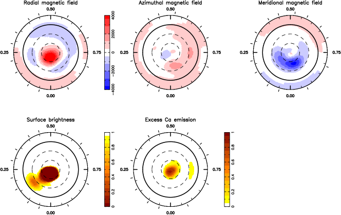
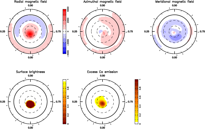
Figure 9: Maps of the radial, azimuthal and meridional components of the magnetic field $\bf B$ (first and third rows, left to right panels respectively), photospheric brightness and excess Ca ii IRT emission (second and fourth rows, first and second panels respectively) at the surface of GQ Lup, in 2009 July (top two rows) and 2011 June (bottom two rows). Magnetic fluxes are labelled in G; local photospheric brightness (normalized to that of the quiet photosphere) varies from 1 (no spot) to 0 (no light); local excess Ca ii emission varies from 0 (no excess emission) to 1 (excess emission covering 100% of the local grid cell, assuming an intrinsic excess emission of 10$\times$ the quiet chromospheric emission). In all panels, the star is shown in flattened polar projection down to latitudes of $-30\hbox{${}^{\circ}$}$, with the equator depicted as a bold circle and parallels as dashed circles. Radial ticks around each plot indicate phases of observations.

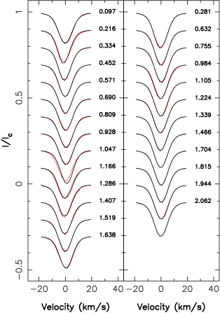
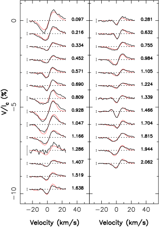
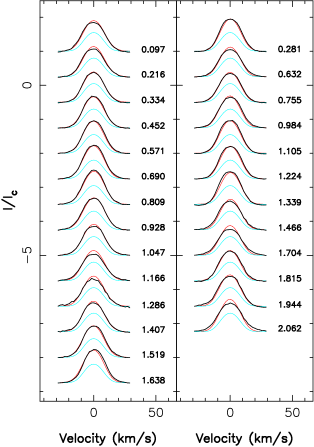
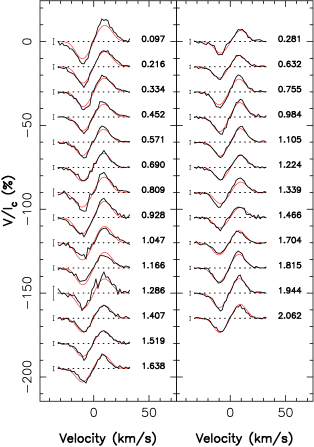
Figure 10: Maximum-entropy fit (thin red line) to the observed (thick black line) Stokes $I$ and Stokes $V$ LSD photospheric profiles (top panels) and Ca ii IRT profiles (bottom panels) of GQ Lup. In each panel, the left and right columns correspond to the 2009 July and 2011 June data respectively. The light-blue curve in the bottom left panel shows the (constant) contribution of the quiet chromosphere to the Stokes $I$ Ca ii profiles. Rotational cycles and 3$\sigma$ error bars (for Stokes $V$ profiles) are also shown next to each profile.

The magnetic, brightness and accretion maps we reconstruct for GQ Lup at both epochs are shown in Fig. 9, with the corresponding fits to the data shown in Fig. 10. The spherical harmonic (SH) expansions describing the field was limited to terms with $\ell\leq 7$, which is found to be adequate when $v\sin i$ is low. The magnetic topology of GQ Lup was also assumed to be antisymmetric with respect to the centre of the star, as in most previous studies.

Error bars on Zeeman signatures were artificially expanded by a factor of 2 (both for LSD profiles and for Ca ii emission and at both epochs) to take into account the level of intrinsic variability (obvious from the lower panels of Figs. 3 and 4, where the observed dispersion on longitudinal fields is larger than formal error bars) and to avoid the code attempting to overfit the data. The fits we finally obtain correspond to a reduced chi-square $\chi^{2}_{\rm r}$ equal to 1, starting from initial values of 16 at both epochs (corresponding to a null magnetic field and unspotted brightness and accretion maps, and with scaled-up error bars on Zeeman signatures).

As a by-product, we obtain new estimates for various spectral characteristics of GQ Lup. In particular, we find that the average RV of GQ Lup has changed from –3.2 from –2.8 km s^-1 between 2009 July and 2011 June; we believe that this change, about 4 times larger than the (conservative) error bar on each measurement, is real. We also find that $v\sin i$ is equal to $5\pm 1$ km s^-1; this is slightly smaller that the best estimate available in the literature (equal to $6.8\pm 0.4$ km s^-1, Guenther et al., 2005), though presumably more accurate (despite the larger error bar) since magnetic broadening (significant in GQ Lup) is taken into account in our study (and not in the former one). We find no clear evidence that GQ Lup is not rotating rigidly; the method previously used for estimating differential rotation on V2129 Oph (Donati et al., 2011a) is much less sensitive for GQ Lup (given the lower inclination angle and the lower $v\sin i$) and remains inconclusive.

Finally, we find that the profiles are best fitted for values of the local filling factor $\psi$ (describing the relative proportion of magnetic areas at any given point of the stellar surface, see Donati et al., 2010) equal to $\simeq$0.3 for LSD profiles and $\simeq$0.6 for Ca ii emission profiles; we obtain in particular that using two different $\psi$ values for the two sets of lines allows an easier fit to the data, although using the same value for both lines (set to $\psi=0.4$, as for all previous cTTSs analysed to date, e.g., Donati et al., 2011a) is still possible (and generates very similar results).

5.2 Modelling results

The large-scale magnetic topology we reconstruct for GQ Lup is mostly axisymmetric at both epochs. It features in particular a region of positive radial field near the pole (see Fig. 9), reaching intensities of up to 5.2 and 4.0 kG in 2009 July and 2011 June respectively, in rough agreement with the peak longitudinal field values probed by the He i emission line (see Fig. 6, lower panels); it also includes an incomplete ring of much weaker negative radial field at low latitudes (see Fig. 9). Both maps also include a conspicuous (though irregular) ring of negative (i.e., equatorward) meridional field located at intermediate latitudes, i.e., between the polar region and low-latitude ring of positive and negative radial field respectively.

The reconstructed field is mostly poloidal, with less that 20% of the reconstructed magnetic energy stored in the toroidal component at either epochs. The poloidal component is mainly axisymmetric, concentrating at least 80–85% of the magnetic energy in SH modes with $m<\ell/2$. More specifically, the poloidal field is found to be dominantly octupolar at both epochs, as obvious from both radial and meridional field maps; the octupole is aligned with the rotation axis to within better than 10^∘ and reaches strengths of 2.4 and 1.6 kG in 2009 July and 2011 June respectively. The large-scale dipole is typically half as intense as the large-scale octupole, with strengths of 1.1 and 0.9 kG in 2009 July and 2011 June (implying octupole to dipole polar strength ratios of 2.2 and 1.8 respectively); it is also more or less parallel (rather than anti-parallel) to the octupole, and is tilted by about 30^∘ to the rotation axis (towards phase 0.05) at both epochs. We can therefore safely confirm that the large-scale field of GQ Lup significantly weakened between 2009 July and 2011 June, as guessed from the long-term evolution of the longitudinal field curves (see Sec. 4); we can further conclude that this variation is mostly attributable to a weakening (by about 1/3) of the octupole component, the overall topology of GQ Lup remaining dominantly octupolar at both epochs.

The reconstructed photospheric brightness distribution mostly features a cool dark spot near the pole (see Fig. 9), shifted by about 20^∘ towards phase 0.05 and occupying about 8% and 4% of the total stellar surface in 2009 July and 2011 June respectively. This cool polar spot mostly overlaps with the visible magnetic pole, as in most other cTTSs magnetically imaged to date; it confirms a posteriori that this is the reason why LSD profiles of photospheric lines are probing field regions of opposite polarity than the accretion lines, i.e., the weakly magnetic low-latitude regions (of negative radial field polarity) rather than the strongly magnetic polar regions (of positive radial field polarity) which emit very few photons per unit area (relative to the rest of the star) and therefore contribute very little to both Stokes $I$ and $V$ LSD profiles. The cool polar spot is found to extend to low latitudes in 2009 July, as expected from the larger amplitude of the RV curve from photospheric lines (see Sec. 4 and Fig. 3, upper panels). We note that synthetic phased curves of RVs and longitudinal fields derived from the reconstructed magnetic and brightness maps are in good agreement with observations at both epochs.

The maps of excess Ca ii emission also show a clear accretion region close to the pole (see Fig. 9), slightly shifted towards phase 0.0 by about 10^∘ and covering $\simeq$2.5% of the stellar surface. We note that, in 2009 July, the accretion map also feature a low-contrast crescent-shape region at low latitudes, centred at phase 0.75; apart from this small difference, the two maps are rather similar, which further demonstrates, at the same time, that the change we report in the longitudinal field curves of accretion proxies (see Sec. 4) unambiguously traces a temporal evolution of the large-scale magnetic topology (and not of the accretion pattern). Unsurprisingly, the synthetic RV curve derived from the 2009 July accretion map, reaching maximum and minimum at phases 0.2 and 0.6 respectively, is found to be more or less in anti-phase with the corresponding observations (see top-left panel of Fig. 4) though both are showing a similarly low peak-to-peak amplitude (of $\simeq$0.5 km s^-1); this confirms the unusual (and yet unexplained) behaviour of the Ca ii RVs at this epoch that we already mentioned in Sec. 4. All other synthetic phased curves (of either equivalent widths, RVs and longitudinal fields) are otherwise in good agreement with observations at both epochs.

6 Summary & discussion

This paper presents the first spectropolarimetric analysis of the cTTS GQ Lup, following previous similar studies of several cTTSs of various masses and ages; this analysis uses extensive data sets collected at two different epochs (2009 July and 2011 June), in the framework of the MaPP Large Program with ESPaDOnS at CFHT. From these data, we start by redetermining the fundamental characteristics of GQ Lup, and in particular its photospheric temperature, found to be $\simeq$250 K warmer than usually quoted in the literature. We also obtain that the rotation period of GQ Lup is $8.4\pm 0.3$ d, in good agreement with the previous estimate of Broeg et al. (2007). We finally conclude that GQ Lup is a $1.05\pm 0.07$ ${\rm M}_{\odot}$ star with an age of 2–5 Myr and a radius of $1.7\pm 0.2$ ${\rm R}_{\odot}$ that has just started to build a radiative core (see Fig 2).

Strong Zeeman signatures are detected at all times in the spectra of GQ Lup, both in LSD profiles of photospheric lines and in emission lines probing accretion regions at the chromospheric level. We report longitudinal fields ranging from –0.1 to –0.6 kG in photospheric lines, from 0.7 to 1.9 kG in the emission core of Ca ii lines, and from 1 to more than 6 kG in the narrow emission profile of He i $D_{3}$ lines, making GQ Lup the cTTS with strongest magnetic fields known as of today. We find in particular that different field polarities are traced by photospheric lines and accretion proxies (as for several other cTTSs), indicating that they probe different spatial regions of GQ Lup. Longitudinal field curves also unambiguously demonstrate that the parent large-scale field of GQ Lup significantly evolved between our two observing runs, with magnetic intensities in accretion regions (where the field is strongest) dropping by as much as 50% between 2009 July and 2011 June; this makes GQ Lup the second cTTS on which temporal evolution of the large-scale magnetic topology has been unambiguously demonstrated (after V2129 Oph, Donati et al., 2011a).

Using our tomographic imaging tool specifically adapted to the case of cTTSs, we convert our two data sets into surface maps of GQ Lup, of the large-scale vector magnetic field on the one hand, and of the photospheric brightness and of the accretion-powered excess emission on the other hand. We find in particular that the large-scale field of GQ Lup is strong, and mostly poloidal and axisymmetric (about the rotation axis). More specifically, we find that the poloidal field is dominated by an octupolar component aligned with the rotation axis (within 10^∘) and whose strength weakens from 2.4 kG in 2009 July to 1.6 kG in 2011 June; we also find that the large-scale dipole of GQ Lup is about half as strong as the octupole, with a polar strength equal to 1.1 and 0.9 kG in 2009 and 2011, and is tilted by $\simeq$30^∘ to the rotation axis (and thus largely parallel, rather than anti-parallel, to the octupole).

The large-scale magnetic topology that we reconstruct for GQ Lup is fully compatible with previous results obtained on cTTSs, suggesting that large-scale fields of protostars hosting small radiative cores are mostly poloidal and axisymmetric, with a dominant octupolar component (e.g., Donati et al., 2011a). This is also similar to that found on main-sequence M dwarfs, where stars with radiative cores smaller than 0.5 $R_{\star}$ host rather strong and mainly poloidal and axisymmetric fields (e.g., Morin et al., 2008, Gregory et al. 2012, submitted). This new result further argues that the magnetic fields of cTTSs are generated through dynamo processes rather than being fossil fields initially present in the parent cloud from which the star has formed and that unexpectedly managed to survive the various turbulent episodes of the cloud-to-disc and disc-to-star contraction phases; clear observational evidence that the large-scale field significantly weakened in a 2 yr timescale independently confirms this conclusion, and indicates at the same time that the underlying dynamo processes are non-stationary.

We also find that the visible pole of GQ Lup (and presumably the invisible pole as well) hosts a cool dark spot at photospheric level and concentrates most of the accreted material from the disc, if we judge from the location of the accretion-powered area of excess Ca ii emission at chromospheric level (roughly overlapping with the cool photospheric spot). These near-polar regions are consistent with the observed low-amplitude RV rotational modulation of photospheric lines and accretion proxies. We also note that additional low-latitude features are detected in 2009 July, both in the photospheric brightness map and in the distribution of accretion-powered emission, suggesting that accretion may also occur (though marginally) at low latitudes at this epoch; a similar conclusion was proposed by Broeg et al. (2007) to attempt reconciling the low inclination of GQ Lup with the large amplitude of its light curve at some epochs. As proposed below, this may be related to the stronger octupolar component of the large-scale magnetic field in the first of our two observing runs.

Given the emission fluxes of the conventional accretion proxies, we infer that the logarithmic mass accretion rate at the surface of GQ Lup is equal to $-9.0\pm 0.3$ (in ${\rm M}_{\odot}$ yr^-1), being slightly stronger (by $\simeq$0.2 dex) in 2009 July than in 2011 June. From this, we infer that GQ Lup should be capable of magnetically disrupting its accretion disc up to a radius of $\hbox{$r_{\rm mag}$}=4.6\pm 1.0$ $R_{\star}$, or equivalently $0.037\pm 0.008$ au (assuming an average dipole strength of 1 kG and using the analytical formula of Bessolaz et al., 2008); in particular, we find that $r_{\rm mag}$ is significantly larger than the radius at which the dipole field starts to dominate over the octupole field (equal to $\simeq$1.2 $R_{\star}$, for an octupole about twice stronger than the dipole, Gregory & Donati, 2011), in agreement with our observation that the accretion flow is mostly poleward on GQ Lup. For larger octupole to dipole polar strength ratios (and when the dipole and octupole are parallel rather than antiparallel), one would naturally expect GQ Lup to trigger increasingly larger amounts of low-latitude accretion (e.g., Romanova et al., 2011); this may be what is happening to GQ Lup in 2009 July, i.e., when the octupole component is strongest and low-contrast low-latitude accretion signatures are being detected. More observations are however necessary to confirm whether observations are consistent with theoretical expectations on this specific issue.

When $r_{\rm mag}$ is compared to the corotation radius $\hbox{$r_{\rm cor}$}\simeq 10.4$ $R_{\star}$ (or 0.083 au), at which the Keplerian period equals the stellar rotation period, we find that $\hbox{$r_{\rm mag}$}/\hbox{$r_{\rm cor}$}$ is equal to $0.45\pm 0.10$, far below the value (of $\simeq 1$) at which star/disc magnetic coupling can start inducing a significant outflow through a propeller-like mechanism (e.g., Romanova et al., 2004) and thus force the star to spin down. We thus speculate that, following the recent build-up of a radiative core and the corresponding change in its large-scale magnetic topology, GQ Lup can no longer counteract the increase of its angular momentum (resulting from both contraction and accretion) through a star-disc braking torque, and has no other option than to undergo a rapid spin up such as that TW Hya experienced already (Donati et al., 2011b). Again, more observations are needed to check these speculations, and in particular to monitor how the magnetic field of the roughly solar-mass GQ Lup is evolving on a longer term (at least on a timescale comparable to that of the solar cycle) and to validate whether the topology we reconstructed from our 2009 and 2011 data sets is indeed typical and adequate to predict the rotational evolution of GQ Lup.

We complete this section by briefly discussing the RV change that we report for GQ Lup, whose average LSD photospheric profile was observed to shift from $-3.2\pm 0.1$ km s^-1 in 2009 July to $-2.8\pm 0.1$ km s^-1 in 2011 June, much larger in particular than spurious shifts potentially attributable to instrument stability problems. Being comparable to the semi-amplitude of the activity-induced modulation of the RV curve (and readily visible from the plots themselves, see Fig. 3, upper panels), this change is also undoubtedly too large to be realistically attributed to uncorrected residuals of RV effects induced by cool spot patterns at the surface of GQ Lup. Various possibilities thus remain to explain it. The first option is that it is caused by long-term changes of the surface convection / granulation pattern; although 0.4 km s^-1 may sound fairly large (for a Sun-like star), little is known in practice about how much this effect can modify RVs in stars as active as cTTSs. The second option is that it is caused by an additional body orbiting GQ Lup, on a timescale of months or years. We already know that GQ Lup is orbited by a brown dwarf (Neuhäuser et al., 2005; McElwain et al., 2007; Lavigne et al., 2009), but its distance from GQ Lup (about 100 au) is likely too large to induce a RV shift similar to the one we report here in a timescale of only 2 yr; this may suggest that GQ Lup hosts a third body much closer to the central protostar than GQ Lup B, e.g., a brown dwarf of a few tens of Jupiter masses at a distance of a few au’s. Additional observations of GQ Lup similar to those presented here are obviously needed to confirm which option applies.

References

- Alencar et al. (2012) Alencar S. H. P., Bouvier J., Walter F., Dougados C., Donati J.-F., Kurosawa R., Romanova M. M., Bonfils X., Lima G., Massaro S., Ibrahimov M., Poretti E., 2012, A&A, p. in press
- André et al. (2009) André P., Basu S., Inutsuka S., 2009, The formation and evolution of prestellar cores. Cambridge University Press, pp 254
- Batalha et al. (2001) Batalha C., Lopes D. F., Batalha N. M., 2001, ApJ, 548, 377
- Bessell et al. (1998) Bessell M. S., Castelli F., Plez B., 1998, A&A, 333, 231
- Bessolaz et al. (2008) Bessolaz N., Zanni C., Ferreira J., Keppens R., Bouvier J., 2008, A&A, 478, 155
- Bouvier et al. (2007b) Bouvier J., Alencar S. H. P., Boutelier T., Dougados C., Balog Z., Grankin K., Hodgkin S. T., Ibrahimov M. A., Kun M., Magakian T. Y., Pinte C., 2007b, A&A, 463, 1017
- Bouvier et al. (2007a) Bouvier J., Alencar S. H. P., Harries T. J., Johns-Krull C. M., Romanova M. M., 2007a, in Reipurth B., Jewitt D., Keil K., eds, Protostars and Planets V Magnetospheric Accretion in Classical T Tauri Stars. pp 479–494
- Broeg et al. (2007) Broeg C., Schmidt T. O. B., Guenther E., Gaedke A., Bedalov A., Neuhäuser R., Walter F. M., 2007, A&A, 468, 1039
- Cieza et al. (2010) Cieza L. A., Schreiber M. R., Romero G. A., Mora M. D., Merin B., Swift J. J., Orellana M., Williams J. P., Harvey P. M., Evans N. J., 2010, ApJ, 712, 925
- Covino et al. (1992) Covino E., Terranegra L., Franchini M., Chavarria-K. C., Stalio R., 1992, A&AS, 94, 273
- Crawford (2000) Crawford I. A., 2000, MNRAS, 317, 996
- Curran et al. (2011) Curran R. L., Argiroffi C., Sacco G. G., Orlando S., Peres G., Reale F., Maggio A., 2011, A&A, 526, A104
- Donati et al. (2011a) Donati J., Bouvier J., Walter F. M., Gregory S. G., Skelly M. B., Hussain G. A. J., Flaccomio E., Argiroffi C., Grankin K. N., Jardine M. M., Ménard F., Dougados C., Romanova M. M., 2011a, MNRAS, 412, 2454
- Donati & Landstreet (2009) Donati J., Landstreet J. D., 2009, ARA&A, 47, 333
- Donati et al. (2010) Donati J., Skelly M. B., Bouvier J., Gregory S. G., Grankin K. N., Jardine M. M., Hussain G. A. J., Ménard F., Dougados C., Unruh Y., Mohanty S., Aurière M., Morin J., Farès R., 2010, MNRAS, 409, 1347
- Donati (2003) Donati J.-F., 2003, in Trujillo-Bueno J., Sanchez Almeida J., eds, Astronomical Society of the Pacific Conference Series Vol. 307 of Astronomical Society of the Pacific Conference Series, ESPaDOnS: An Echelle SpectroPolarimetric Device for the Observation of Stars at CFHT. pp 41
- Donati et al. (2011b) Donati J.-F., Gregory S. G., Alencar S. H. P., Bouvier J., Hussain G., Skelly M., Dougados C., Jardine M. M., Ménard F., Romanova M. M., Unruh Y. C., 2011b, MNRAS, 417, 472
- Donati et al. (2006) Donati J.-F., Howarth I. D., Jardine M. M., Petit P., Catala C., Landstreet J. D., Bouret J.-C., Alecian E., Barnes J. R., Forveille T., Paletou F., Manset N., 2006, MNRAS, 370, 629
- Donati et al. (2007) Donati J.-F., Jardine M. M., Gregory S. G., Petit P., Bouvier J., Dougados C., Ménard F., Cameron A. C., Harries T. J., Jeffers S. V., Paletou F., 2007, MNRAS, 380, 1297
- Donati et al. (2008a) Donati J.-F., Jardine M. M., Gregory S. G., Petit P., Paletou F., Bouvier J., Dougados C., Ménard F., Cameron A. C., Harries T. J., Hussain G. A. J., Unruh Y., Morin J., Marsden S. C., Manset N., Aurière M., Catala C., Alecian E., 2008a, MNRAS, 386, 1234
- Donati et al. (2008b) Donati J.-F., Moutou C., Farès R., Bohlender D., Catala C., Deleuil M., Shkolnik E., Cameron A. C., Jardine M. M., Walker G. A. H., 2008b, MNRAS, 385, 1179
- Donati et al. (1997) Donati J.-F., Semel M., Carter B. D., Rees D. E., Collier Cameron A., 1997, MNRAS, 291, 658
- Fang et al. (2009) Fang M., van Boekel R., Wang W., Carmona A., Sicilia-Aguilar A., Henning T., 2009, A&A, 504, 461
- Gregory & Donati (2011) Gregory S. G., Donati J.-F., 2011, Astronomische Nachrichten, 332, 1027
- Gregory et al. (2010) Gregory S. G., Jardine M., Gray C. G., Donati J., 2010, Reports on Progress in Physics, 73, 126901
- Gregory et al. (2008) Gregory S. G., Matt S. P., Donati J.-F., Jardine M., 2008, MNRAS, 389, 1839
- Guenther et al. (2005) Guenther E. W., Neuhäuser R., Wuchterl G., Mugrauer M., Bedalov A., Hauschildt P. H., 2005, Astronomische Nachrichten, 326, 958
- Janson et al. (2006) Janson M., Brandner W., Henning T., Zinnecker H., 2006, A&A, 453, 609
- Johns-Krull (2007) Johns-Krull C. M., 2007, ApJ, 664, 975
- Kurucz (1993) Kurucz R., 1993, CDROM # 13 (ATLAS9 atmospheric models) and # 18 (ATLAS9 and SYNTHE routines, spectral line database). Smithsonian Astrophysical Observatory, Washington D.C.
- Landi degl’Innocenti & Landolfi (2004) Landi degl’Innocenti E., Landolfi M., 2004, Polarisation in spectral lines. Dordrecht/Boston/London: Kluwer Academic Publishers
- Lavigne et al. (2009) Lavigne J.-F., Doyon R., Lafrenière D., Marois C., Barman T., 2009, ApJ, 704, 1098
- Long et al. (2008) Long M., Romanova M. M., Lovelace R. V. E., 2008, MNRAS, 386, 1274
- McElwain et al. (2007) McElwain M. W., Metchev S. A., Larkin J. E., Barczys M., Iserlohe C., Krabbe A., Quirrenbach A., Weiss J., Wright S. A., 2007, ApJ, 656, 505
- Morin et al. (2008) Morin J., Donati J.-F., Petit P., Delfosse X., Forveille T., Albert L., Aurière M., Cabanac R., Dintrans B., Fares R., Gastine T., Jardine M. M., Lignières F., Paletou F., Ramirez Velez J. C., Théado S., 2008, MNRAS, 390, 567
- Natta et al. (2004) Natta A., Testi L., Muzerolle J., Randich S., Comerón F., Persi P., 2004, A&A, 424, 603
- Neuhäuser et al. (2005) Neuhäuser R., Guenther E. W., Wuchterl G., Mugrauer M., Bedalov A., Hauschildt P. H., 2005, A&A, 435, L13
- Romanova et al. (2011) Romanova M. M., Long M., Lamb F. K., Kulkarni A. K., Donati J., 2011, MNRAS, 411, 915
- Romanova et al. (2004) Romanova M. M., Ustyugova G. V., Koldoba A. V., Lovelace R. V. E., 2004, ApJL, 616, L151
- Seperuelo Duarte et al. (2008) Seperuelo Duarte E., Alencar S. H. P., Batalha C., Lopes D., 2008, A&A, 489, 349
- Siess et al. (2000) Siess L., Dufour E., Forestini M., 2000, A&A, 358, 593
- Valenti & Fischer (2005) Valenti J. A., Fischer D. A., 2005, ApJS, 159, 141
- Wichmann et al. (1999) Wichmann R., Covino E., Alcalá J. M., Krautter J., Allain S., Hauschildt P. H., 1999, MNRAS, 307, 909