Image quality in double- and triple-intensity ghost imaging
with classical partially polarized light

Abstract

Classical ghost imaging is a correlation-imaging technique in which the image of the object is found through intensity correlations of light. We analyze three different quality parameters, namely the visibility, the signal-to-noise ratio (SNR), and the contrast-to-noise ratio (CNR), to assess the performance of double- and triple-intensity correlation-imaging setups. The source is a random partially polarized beam of light obeying Gaussian statistics and the image quality is evaluated as a function of the degree of polarization (DoP). We show that the visibility improves when the DoP and the order of imaging increase, while the SNR behaves oppositely. The CNR is for the most part independent of the DoP and the imaging order. The results are important for the development of new imaging devices using partially polarized light.

¹Department of Applied Physics, Aalto University, P. O. Box 13500, FI-00076 Aalto, Finland

²Electronics and Photonics Research Institute, National Institute of Advanced Industrial Science and Technology, AIST Tsukuba Central 2, 1-1-1 Umezono, Tsukuba 305-8568, Japan

³Department of Physics and Mathematics, University of Eastern Finland, P. O. Box 111, FI-80101 Joensuu, Finland

⁴Department of Microelectronics and Applied Physics, Royal Institute of Technology, Electrum 229, SE-164 40 Kista, Sweden

^∗Corresponding author: henri.kellock@aalto.fi

March 7, 2024

1 Introduction

Ghost imaging, or correlation imaging, is a novel imaging technique in which information about the object is found through photon coincidences or classical light correlations [1, 2]. Originally demonstrated with entangled photon pairs providing a high-visibility image [3, 4], ghost imaging has since been realized with classically correlated [5] and incoherent (quasi-thermal) light [6, 7]. Recently it has been extended to imaging of temporal objects [8, 9, 10], of pure phase objects [11], and through aberrations [12, 13, 14, 15, 16]. Essential features of quantum ghost imaging can be emulated with classical light, apart from the visibility as there is a constant background present in classical imaging [17, 6, 7, 18, 19]. The advantages of classical light are higher brightness and readily available sources. Various techniques have been introduced to improve the image quality in ghost imaging. These include use of higher-order correlations [20, 21], background subtraction [22], differential ghost imaging [23], and computational ghost imaging [24, 25].

The signal in ghost imaging is noisy and several parameters have been used to characterize the image quality. Two definitions are typically employed for visibility [6, 20]. Besides visibility, the signal-to-noise ratio (SNR) and the contrast-to-noise ratio (CNR) characterize image quality and various quantitative measures have been proposed in ghost imaging for both of them [26, 22, 23, 27]. While the visibility characterizes the contrast of the image, the SNR and CNR attempt to take into account the levels of the image noise. Most of the works concerning image quality in ghost or correlation imaging have dealt with scalar radiation and only recently the vectorial nature of light has been considered by studying the effect that partial polarization has on ghost imaging with classical light [28, 29, 30]. In particular, it has been shown that the visibility increases monotonically with the degree of polarization (DoP) [30] and with the order of intensity correlations [28], i.e., the number of arms in the ghost-imaging setup.

In this work we investigate second-order (double-intensity, two arms) and third-order (triple-intensity, three arms) classical ghost imaging with partially polarized light obeying Gaussian statistics. Specifically, we analyze the image quality in terms of the visibility, SNR, and CNR. Both a general intensity-correlation arrangement and a specific ghost-imaging setup with lenses and an object in one arm are considered. We show that although the visibility improves with increasing DoP and is also better for third-order ghost imaging, the situation is not so straightforward with the SNR and CNR. On the contrary, due to increased noise, the SNR decreases with the DoP and the order of imaging, while the CNR is largely not affected by either. Owing to the noisy source, the SNR and CNR are generally small, even below one.

The paper is organized as follows. In Sec. 2 we discuss electromagnetic intensity correlations and introduce the double- and triple-intensity ghost-imaging arrangements that we consider. In Sec. 3 we analyse the visibility in these setups and in Secs. 4 and 5 we calculate the corresponding SNR and CNR, respectively. A summary and a brief discussion of our results and their consequences are presented in Sec. 6. Some mathematical details are relegated to Appendices A–C.

2 Electromagnetic correlation imaging

We begin by considering intensity correlation functions (ICFs) of $N$ random electromagnetic intensities corresponding to fields obeying joint Gaussian statistics. We then describe the second-order (double-intensity) and third-order (triple-intensity) correlation-imaging setups. In both cases we first introduce a general intensity-correlation arrangement and then particularize it to ghost imaging with one object arm.

2.1 Degree of polarization

Consider a stationary, uniformly polarized random beam of light propagating in the direction of the $z$-axis with the electric field lying in the $xy$-plane. The beam’s polarization state is characterized by the polarization matrix [31]

$$\mathbf{J}_{0}=\left[\begin{array}[]{cc}J_{xx}&J_{xy}\\ J_{yx}&J_{yy}\end{array}\right],$$ (1)

where $J_{ij}=\left\langle E_{i}^{*}(t)E_{j}(t)\right\rangle$, $i,j\in\left\{x,y\right\}$, is the correlation function between the electric-field components and $\left\langle\ldots\right\rangle$ denotes the time (or ensemble) average. Due to the Hermiticity and non-negative definiteness of $\mathbf{J}_{0}$ there always exists a unitary transformation which diagonalizes $\mathbf{J}_{0}$ and the eigenvalues $J_{1}$ and $J_{2}$ are non-negative. Choosing $J_{1}\geq J_{2}$ the degree of polarization (DoP) is

$$P=\frac{J_{1}-J_{2}}{J_{1}+J_{2}}.$$ (2)

This expression is mathematically identical to the ones obtained by dividing the beam into fully polarized and unpolarized parts and defining $P$ as the ratio between the energy of the fully polarized component and that of the total beam [31]. Thus, when the light is completely polarized $P=1$, unpolarized light has $P=0$, and all other states are partially polarized.

2.2 Intensity correlations

The equal-time intensity correlation function (ICF) between $N$ optical intensities is given by [32, 31]

$$G^{(N)}(\mathbf{r}_{1},\ldots,\mathbf{r}_{N})=\left\langle I_{1}\cdots I_{N}\right\rangle,$$ (3)

where $I_{\alpha}=\mathbf{E}_{\alpha}^{*}(\mathbf{r}_{\alpha},t)\cdot\mathbf{E}_{\alpha}(\mathbf{r}_{\alpha},t)$ with $\alpha\in\{1,\ldots,N\}$ is the instantaneous intensity at point $\mathbf{r}_{\alpha}$. For stationary light the equal-time ICFs are independent of time but depend on position. The normalized version of $G^{(N)}$ is

$$g^{(N)}\equiv\frac{\left\langle I_{1}\cdots I_{N}\right\rangle}{\left\langle I_{1}\right\rangle\cdots\left\langle I_{N}\right\rangle},$$ (4)

which will be of convenience later. Each intensity can be expressed as $I_{\alpha}=I_{\alpha x}+I_{\alpha y}=\left|E_{\alpha,x}(\mathbf{r}_{\alpha},t)\right|^{2}+\left|E_{\alpha,y}(\mathbf{r}_{\alpha},t)\right|^{2}$, where $E_{\alpha,x}(\mathbf{r}_{\alpha},t)$ and $E_{\alpha,y}(\mathbf{r}_{\alpha},t)$ are, respectively, the $x$- and $y$-components of the electric field. Thus the $N$th-order intensity correlation function can be divided into a sum of the $N$th-order ICFs of the different components as [28]

$$\left\langle I_{1}\cdots I_{N}\right\rangle=\sum_{i_{1},\ldots,i_{N}\in\{x,y\}}\left\langle I_{1i_{1}}\cdots I_{Ni_{N}}\right\rangle,$$ (5)

where the sum is taken over $i_{\alpha}\in\{x,y\}$ for all $\alpha\in\{1,\ldots,N\}$. Due to the underlying Gaussian statistics, we may apply the moment theorem and obtain [31, 20]

$$\left\langle I_{1i_{1}}\cdots I_{Ni_{N}}\right\rangle=\sum_{N!}\Gamma_{i_{1}\underline{i_{1}}}^{1\underline{1}}\cdots\Gamma_{i_{N}\underline{i_{N}}}^{N\underline{N}},$$ (6)

where the summation is performed over all the $N!$ possible permutations of the underlined indices and $\Gamma_{ij}^{\alpha\beta}\equiv\bigl{\langle}E_{\alpha,i}^{*}(\mathbf{r}_{\alpha},t)E_{\beta,j}(\mathbf{r}_{\beta},t)\bigr{\rangle},$ with $i,j\in\{x,y\}$ and $\alpha,\beta\in\{1,\ldots,N\}$, is the correlation function between the electric-field components.

We can express the $N$th-order ICF in terms of the equal-time mutual coherence (or the mutual intensity) matrix

$$\mathbf{\Gamma}^{\alpha\beta}=\left[\begin{array}[]{cc}\Gamma_{xx}^{\alpha\beta}&\Gamma_{xy}^{\alpha\beta}\\ \Gamma_{yx}^{\alpha\beta}&\Gamma_{yy}^{\alpha\beta}\end{array}\right],$$ (7)

where the elements are defined as above. In the second-order we find that

$$\left\langle I_{1}I_{2}\right\rangle=\mathrm{tr}\mathbf{\Gamma}^{11}\mathrm{tr}\mathbf{\Gamma}^{22}+\mathrm{tr}(\mathbf{\Gamma}^{12}\mathbf{\Gamma}^{21}),$$ (8)

where $\mathrm{tr}$ denotes the trace and $\mathrm{tr}\mathbf{\Gamma}^{\alpha\alpha}=\left\langle I_{\alpha}\right\rangle$ is the $\alpha$th average intensity. The first term is the product of the mean intensities $\left\langle I_{1}\right\rangle\left\langle I_{2}\right\rangle$ and the second one is the correlation of the intensity fluctuations $\left\langle\Delta I_{1}\Delta I_{2}\right\rangle$, where $\Delta I_{\alpha}=I_{\alpha}-\left\langle I_{\alpha}\right\rangle$ with $\alpha\in\{1,2\}$. It is the latter term that is responsible for image formation in ghost imaging. Similarly, the third-order ICF takes on the form

$$\left\langle I_{1}I_{2}I_{3}\right\rangle =\mathrm{tr}\mathbf{\Gamma}^{11}\mathrm{tr}\mathbf{\Gamma}^{22}\mathrm{tr}\mathbf{\Gamma}^{33}+\mathrm{tr}\mathbf{\Gamma}^{33}\mathrm{tr}(\mathbf{\Gamma}^{12}\mathbf{\Gamma}^{21})$$

$$+\mathrm{tr}\mathbf{\Gamma}^{22}\mathrm{tr}(\mathbf{\Gamma}^{13}\mathbf{\Gamma}^{31})+\mathrm{tr}\mathbf{\Gamma}^{11}\mathrm{tr}(\mathbf{\Gamma}^{23}\mathbf{\Gamma}^{32})$$

$$+\mathrm{tr}(\mathbf{\Gamma}^{12}\mathbf{\Gamma}^{23}\mathbf{\Gamma}^{31})+\mathrm{tr}(\mathbf{\Gamma}^{13}\mathbf{\Gamma}^{32}\mathbf{\Gamma}^{21}).$$ (9)

The first term is again the product of the mean intensities $\left\langle I_{1}\right\rangle\left\langle I_{2}\right\rangle\left\langle I_{3}\right\rangle$, the next three terms have a mean intensity multiplied by the correlation of intensity fluctuations between the remaining two intensities, e.g., $\left\langle I_{3}\right\rangle\left\langle\Delta I_{1}\Delta I_{2}\right\rangle$, and the sum of the last two terms is equal to the correlation of all the intensity fluctuations $\left\langle\Delta I_{1}\Delta I_{2}\Delta I_{3}\right\rangle$.

2.3 Double-intensity correlation imaging

A general second-order correlation imaging geometry is depicted in Fig. 1(a). The source is a classical, quasi-monochromatic, uniformly partially polarized electromagnetic beam of light represented by the mutual intensity matrix $\mathbf{\Gamma}_{0}(\mathbf{r}_{1}^{\prime},\mathbf{r}_{2}^{\prime})=\mathbf{J}_{0}\gamma_{0}(\mathbf{r}_{1}^{\prime},\mathbf{r}_{2}^{\prime})$, where $\mathbf{J}_{0}$ is the polarization matrix and $\gamma_{0}(\mathbf{r}_{1}^{\prime},\mathbf{r}_{2}^{\prime})$ is a normalized spatial coherence function. The source beam is split into two arms and propagated along the paths described by the kernels $K_{1}$ and $K_{2}$. The arms are taken to be polarization independent and their properties do not vary with time. The intensities $I_{1}$ and $I_{2}$ at the end of the paths are measured as a function of position and correlated producing $\left\langle I_{1}I_{2}\right\rangle$.

The intensity correlation is given by Eq. (8). The mutual intensity matrices appearing in this equation can be written as [29, 30]

$$\mathbf{\Gamma}^{\alpha\beta}=\mathbf{J}_{0}\hat{\Gamma}^{\alpha\beta},$$ (10)

where

$$\hat{\Gamma}^{\alpha\beta}=\iint\gamma_{0}(\mathbf{r}_{1}^{\prime},\mathbf{r}_{2}^{\prime})K_{\alpha}^{*}(\mathbf{r}_{\alpha},\mathbf{r}_{1}^{\prime})K_{\beta}(\mathbf{r}_{\beta},\mathbf{r}_{2}^{\prime})\mathrm{d}\mathbf{r}_{1}^{\prime}\mathrm{d}\mathbf{r}_{2}^{\prime}$$ (11)

with $\alpha,\beta\in\left\{1,2\right\}$. Here and henceforth the primed coordinates refer to the source plane and the coordinates $\mathbf{r}_{\alpha}$ refer to the plane of the detector in arm $\alpha$. We define the normalized form of $\hat{\Gamma}^{\alpha\beta}$ as

$$\hat{\gamma}^{\alpha\beta}\equiv\hat{\Gamma}^{\alpha\beta}/\sqrt{\hat{\Gamma}^{\alpha\alpha}\hat{\Gamma}^{\beta\beta}},$$ (12)

which in view of the Schwarz inequality satisfies $0\leq|\hat{\gamma}^{\alpha\beta}|\leq 1$. Inserting Eq. (10) into Eq. (8) and employing Eqs. (4) and (12) gives the normalized intensity correlation function

$$g^{(2)}(\mathbf{r}_{1},\mathbf{r}_{2})=1+\frac{P^{2}+1}{2}\left|\hat{\gamma}^{12}\right|^{2},$$ (13)

where we used Eq. (A.4) of Appendix A. The quantity $g^{(2)}$ has a constant background and a term that contains information on the correlation of the intensities $I_{1}$ and $I_{2}$ and depends on the degree of polarization $P$.

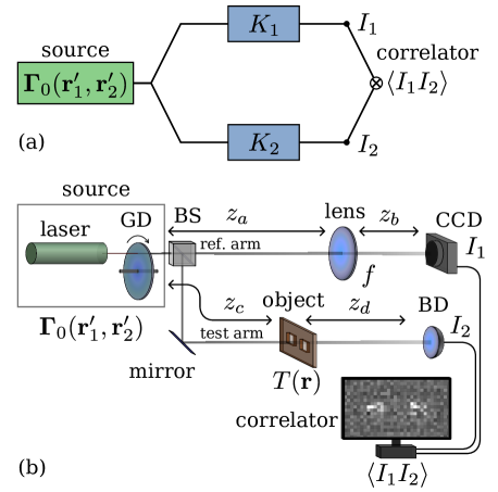
Figure 1: (a) Generic and (b) specific double-intensity correlation-imaging setups. In (a), the source beam [$\mathbf{\Gamma}_{0}(\mathbf{r}_{1}^{\prime},\mathbf{r}_{2}^{\prime})$] is split into two arms characterized by the kernels $K_{1}$ and $K_{2}$. The beam intensities $I_{1}$ and $I_{2}$ at the end of the arms are measured and correlated ($\left\langle I_{1}I_{2}\right\rangle$). In (b), a laser and a rotating ground glass disk (GD) are used to create a spatially incoherent light beam which then is divided into two arms with a beam splitter (BS). The reference arm has a lens with the focal length $f$ and the test arm contains the object with the transmission function $T(\mathbf{r})$. The propagation distances are denoted by $z_{i}$, $i\in\{a,b,c,d\}$. The reference arm has a CCD camera to measure the intensity distribution and the test arm includes a bucket detector (BD) which measures the total intensity. An intensity correlation ($\left\langle I_{1}I_{2}\right\rangle$) is performed to form an image of the object.

Double-intensity ghost-imaging setup

We now consider the specific ghost-imaging setup shown in Fig. 1(b). The source is spatially completely incoherent, characterized by the mutual intensity matrix $\mathbf{\Gamma}_{0}(\mathbf{r}_{1}^{\prime},\mathbf{r}_{2}^{\prime})=\mathbf{J}_{0}\delta(\mathbf{r}_{2}^{\prime}-\mathbf{r}_{1}^{\prime})$, where $\delta$ is the Dirac delta function. In addition, the reference arm ($K_{1}$) contains a lens and a high-resolution detector, and the test arm ($K_{2}$) includes the object and a bucket detector with no spatial resolution.

For a thin and large-aperture lens, the reference arm is described by the kernel [33]

$$K_{1}(\mathbf{r}_{1},\mathbf{r}_{1}^{\prime}) =\frac{i}{\lambda\zeta}\exp\left\{\frac{ik}{2\zeta}\left[\left(\mathbf{r}_{1}^{\prime}-\mathbf{r}_{1}\right)^{2}-\frac{z_{b}{\mathbf{r}_{1}^{\prime}}^{2}+z_{a}\mathbf{r}_{1}^{2}}{f}\right]\right\},$$ (14)

where $z_{a}$ and $z_{b}$ are the propagation distances, $f$ is the lens focal length, $\zeta\equiv z_{a}+z_{b}-z_{a}z_{b}/f$, and $k=2\pi/\lambda$ is the wave number, with $\lambda$ being the wavelength. The transmission function $T(\mathbf{r})$ characterizes the object, which is preceded with the propagation distance $z_{c}$ and succeeded with $z_{d}$. The kernel of the test arm is

$$K_{2}(\mathbf{r}_{2},\mathbf{r}_{2}^{\prime})$$

$$=\frac{1}{\lambda^{2}z_{a}z_{b}}\int T(\mathbf{r})\exp\left\{\frac{ik}{2}\left[\frac{\left(\mathbf{r}-\mathbf{r}_{2}^{\prime}\right)^{2}}{z_{c}}+\frac{\left(\mathbf{r}_{2}-\mathbf{r}\right)^{2}}{z_{d}}\right]\right\}\mathrm{d}\mathbf{r}.$$ (15)

The normalized correlation between the output intensities is given by Eq. (13), where $\hat{\gamma}^{12}$ is specified by [see Eqs. (11) and (12)]

$$\hat{\Gamma}^{\alpha\beta}=\int K_{\alpha}^{*}(\mathbf{r}_{\alpha},\mathbf{r}^{\prime})K_{\beta}(\mathbf{r}_{\beta},\mathbf{r}^{\prime})\mathrm{d}\mathbf{r}^{\prime}$$ (16)

with $\alpha,\beta\in\{1,2\}$. If the imaging condition [34, 35]

$$\frac{1}{f}=\frac{1}{z_{a}-z_{c}}+\frac{1}{z_{b}}$$ (17)

holds, we find with the use of Eqs. (14)–(17) that

$$\left|\hat{\Gamma}^{12}\right|^{2}=\frac{\left(z_{a}-z_{c}\right)^{2}}{\lambda^{2}z_{b}^{2}z_{d}^{2}}\left|T(-\frac{z_{a}-z_{c}}{z_{b}}\mathbf{r}_{1})\right|^{2}.$$ (18)

Thus an intensity correlation measurement can form an image (of the absolute value) of the object. The image is not due to the output intensities [$\mathrm{tr}\mathbf{\Gamma}^{11}$, $\mathrm{tr}\mathbf{\Gamma}^{22}$ in Eq. (8)] but rather results from the correlation of the intensity fluctuations at the outputs [$\mathrm{tr}(\mathbf{\Gamma}^{12}\mathbf{\Gamma}^{21})$]. Since $0\leq|\hat{\gamma}^{12}|\leq 1$, the normalized output intensity correlation is in the range $1\leq g^{(2)}\leq\left(P^{2}+3\right)/2$ suggesting that the image quality depends on the DoP. The range of $g^{(2)}$ holds both for the general geometry of Fig. 1(a) and for the specific setup shown in Fig. 1(b) indicating that they have the same image quality.

2.4 Triple-intensity correlation imaging

A general third-order correlation imaging geometry containing three arms described by the kernels $K_{1}$, $K_{2}$, and $K_{3}$ is depicted in Fig. 2(a). We make the same assumptions about the source ($\mathbf{\Gamma}_{0}$) and the arms as in the second-order case analyzed in the beginning of Sec. 2.3. The correlation of the intensities at the end of the arms, $\left\langle I_{1}I_{2}I_{3}\right\rangle$, is provided by Eq. (9). The mutual intensity matrices appearing in this equation satisfy Eqs. (10) and (11) with $\alpha,\beta\in\{1,2,3\}$. These equations together with Eqs. (4), (9), (12), and (A.4) give the normalized triple-intensity ICF

$$g^{(3)}(\mathbf{r}_{1},\mathbf{r}_{2},\mathbf{r}_{3}) =1+\frac{P^{2}+1}{2}(\left|\hat{\gamma}^{12}\right|^{2}+\left|\hat{\gamma}^{13}\right|^{2}+\left|\hat{\gamma}^{23}\right|^{2})$$

$$+\frac{3P^{2}+1}{2}\Re(\hat{\gamma}^{12}\hat{\gamma}^{23}\hat{\gamma}^{31}),$$ (19)

where $\Re(\ldots)$ denotes the real part. We can express the complex correlation coefficients in terms of their magnitudes and phases as $\hat{\gamma}^{\alpha\beta}=|\hat{\gamma}^{\alpha\beta}|e^{i\phi_{\alpha\beta}}$. This implies that $\Re(\hat{\gamma}^{12}\hat{\gamma}^{23}\hat{\gamma}^{31})=|\hat{\gamma}^{12}||\hat{\gamma}^{23}||\hat{\gamma}^{13}|\cos(\Delta\phi_{123})$, where we have introduced the notation $\Delta\phi_{123}\equiv\phi_{12}+\phi_{23}-\phi_{13}$ and used the fact that $(\hat{\gamma}^{\alpha\beta})^{*}=\hat{\gamma}^{\beta\alpha}$. The function $g^{(3)}$ has a constant background (equal to one) followed by three DoP-dependent terms which each contain information on the correlation of a different pair of fields [21]. The last term has the strongest dependence on $P$ and it carries information on all the three correlations. Because $0\leq|\hat{\gamma}^{\alpha\beta}|\leq 1$ for all $\alpha,\beta\in\{1,2,3\}$, the normalized third-order ICF is in the range $1\leq g^{(3)}\leq 3P^{2}+3$ suggesting, as in the second-order case, that the image quality depends in an essectial way on the DoP of the source.

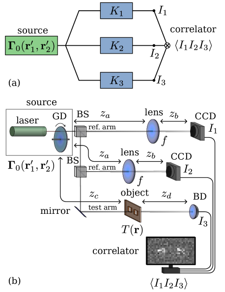
Figure 2: (a) Generic and (b) specific triple-intensity correlation imaging setups. Part (a) is similar to Fig. 1(a) but has three arms instead of two. Likewise, part (b) is analogous to Fig. 1(b) with the exception that there is an additional reference arm which is identical to the first one.

Triple-intensity setup with one object arm

As the last arrangement, we consider the specific third-order ghost-imaging scheme shown in Fig. 2(b). The source ($\mathbf{\Gamma}_{0}$), the reference arms [$K_{1}$ and $K_{2}$, as expressed in Eq. (14)], and the test arm [$K_{3}$, see Eq. (15)] are as in the specific double-intensity ghost-imaging setup of Sec. 2.3. The normalized ICF of the outputs is given by Eq. (19), where the functions $\hat{\gamma}^{\alpha\beta}$ are obtained from Eqs. (12) and (16) with $\alpha,\beta\in\{1,2,3\}$.

Since both reference arms are the same, the correlation function between them is

$$\hat{\Gamma}^{12} =\exp\left\{\frac{ik}{2}\left[\frac{1-z_{a}/f}{\zeta}\left(\mathbf{r}_{2}^{2}-\mathbf{r}_{1}^{2}\right)\right]\right\}\delta\left(\mathbf{r}_{1}-\mathbf{r}_{2}\right),$$ (20)

where the parameters are the same as those in Eq. (14). The Dirac delta function in this equation is due to the spatially fully incoherent source. Physically $\hat{\Gamma}^{12}$ in Eq. (20) represents complete lack of correlation between the two fields when $\mathbf{r}_{1}\neq\mathbf{r}_{2}$ but shows complete correlation (with a uniform amplitude of unity) when the points are equal. In Appendix B we use a spatially partially coherent source to explicitly demonstrate that the normalized correlation function indeed is $\hat{\gamma}^{12}=1$ when $\mathbf{r}_{1}=\mathbf{r}_{2}$. The remaining correlation quantities $\hat{\Gamma}^{13}$ and $\hat{\Gamma}^{23}$ are equal and given by Eq. (18) as long as the imaging condition of Eq. (17) holds. For $\mathbf{r}_{1}=\mathbf{r}_{2}$ the triple-intensity ICF of Eq. (19) then yields

$$g^{(3)}(\mathbf{r}_{1},\mathbf{r}_{1},\mathbf{r}_{3})=\frac{P^{2}+3}{2}+\frac{5P^{2}+3}{2}\left|\hat{\gamma}^{13}\right|^{2}.$$ (21)

In other words, the information on the object is in the terms $\mathrm{tr}(\mathbf{\Gamma}^{13}\mathbf{\Gamma}^{31})$, $\mathrm{tr}(\mathbf{\Gamma}^{23}\mathbf{\Gamma}^{32})$, $\mathrm{tr}(\mathbf{\Gamma}^{12}\mathbf{\Gamma}^{23}\mathbf{\Gamma}^{31})$, and $\mathrm{tr}(\mathbf{\Gamma}^{13}\mathbf{\Gamma}^{32}\mathbf{\Gamma}^{21})$ of Eq. (9), characterizing the correlations of the intensity fluctuations between the test arm and the reference arms. Because now $\hat{\gamma}^{12}=1$ and $0\leq|\hat{\gamma}^{13}|\leq 1$, the normalized third-order intensity correlation of Eq. (21) is in the range $\left(P^{2}+3\right)/2\leq g^{(3)}\leq 3P^{2}+3$.

3 Visibility

Among the ghost-imaging quality parameters, the visibility of the image has remained as an important quantity, although other parameters have been introduced. Visibility (or image contrast) describes the relative difference between the bright and dark areas of the image. Most studies on visibility in ghost imaging were initially performed in the double-intensity case [6, 19, 1], but higher-order imaging has gained increased attention [20, 26, 36]. Some preliminary works on the influence of the degree of polarization on visibility have been carried out recently [28, 30].

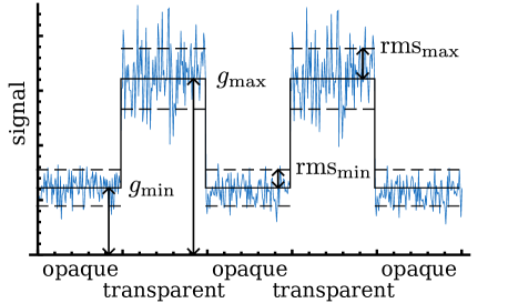
Figure 3: Qualitative sample realization of a normalized ghost-imaging signal. The object has two transparent regions with a normalized mean signal $g_{\mathrm{max}}$ corresponding to the bright areas of the image. The rest of the object is opaque leading to the signal $g_{\mathrm{min}}$ and the dark areas in the image. The noise levels in the bright and dark areas are characterized by the root-mean-square values $\mathrm{rms}_{\mathrm{max}}$ and $\mathrm{rms}_{\mathrm{min}}$ of the fluctuations, respectively.

Two main definitions are in use for the visibility in ghost imaging. The definition employed by Cao et al. [20] for $N$th-order imaging is

$$V_{\mathrm{C}}^{(N)}\equiv\frac{g_{\mathrm{max}}^{(N)}-g_{\mathrm{min}}^{(N)}}{g_{\mathrm{max}}^{(N)}+g_{\mathrm{min}}^{(N)}},$$ (22)

where $g_{\mathrm{max}}^{(N)}$ and $g_{\mathrm{min}}^{(N)}$ can be thought of as the average signal in the bright and dark areas of the ghost image, corresponding to the parts where the object is transparent or opaque, respectively. This idea is illustrated in Fig. 3, where a one-dimensional random realization of a signal related to an object with fully transparent and opaque regions is shown.

The visibility employed by Gatti et al. [19, 1] may be defined for second-order ghost imaging as $V_{\mathrm{G}}^{(2)}\equiv\left\langle\Delta I_{1}\Delta I_{2}\right\rangle_{\mathrm{max}}/\left\langle I_{1}I_{2}\right\rangle_{\mathrm{max}}$. Since $\left\langle I_{1}\right\rangle\left\langle I_{2}\right\rangle$ is a constant background, we obtain

$$V_{\mathrm{G}}^{(2)}=\frac{\left\langle I_{1}I_{2}\right\rangle_{\mathrm{max}}-\left\langle I_{1}\right\rangle\left\langle I_{2}\right\rangle}{\left\langle I_{1}I_{2}\right\rangle_{\mathrm{max}}}=\frac{g_{\mathrm{max}}^{(2)}-1}{g_{\mathrm{max}}^{(2)}}.$$ (23)

There are two principal ways of extending this to higher orders, one of which assumes that $\left\langle I_{1}\cdots I_{N}\right\rangle_{\mathrm{min}}=\left\langle I_{1}\right\rangle\cdots\left\langle I_{N}\right\rangle$ [37] and the other that $\left\langle I_{1}\cdots I_{N}\right\rangle_{\mathrm{min}}=\left\langle I_{1}\cdots I_{N-1}\right\rangle\left\langle I_{N}\right\rangle$ [26]. Translated to the triple-intensity imaging schemes of Fig. 2, the first case corresponds to part (a); the minimum of the ghost-imaging signal is obtained when all intensity-fluctuation correlations disappear and only the first term in Eq. (9) remains. The second case, $\left\langle I_{1}I_{2}I_{3}\right\rangle_{\mathrm{min}}=\left\langle I_{1}I_{2}\right\rangle\left\langle I_{3}\right\rangle$, is closely related to Fig. 2(b), where the intensity correlation between the reference arms [the first two terms in Eq. (9)] contributes to the background, since these beams contain no information about the image. However, we want to take into account all the various arrangements and thus we generalize the definition to the $N$th order as

$$V_{\mathrm{G}}^{(N)}\equiv\frac{\left\langle I_{1}\cdots I_{N}\right\rangle_{\mathrm{max}}-\left\langle I_{1}\cdots I_{N}\right\rangle_{\mathrm{min}}}{\left\langle I_{1}\cdots I_{N}\right\rangle_{\mathrm{max}}}=\frac{g_{\mathrm{max}}^{(N)}-g_{\mathrm{min}}^{(N)}}{g_{\mathrm{max}}^{(N)}}.$$ (24)

The visibilities are normalized so that $0\leq V_{C}^{(N)},V_{G}^{(N)}\leq 1$, but they scale differently between the end points. However, both definitions, Eqs. (22) and (24), can be expected to lead to similar physical conclusions on the image quality. Next we make use of the results from Sec. 2 to calculate these quantities for double- and triple-intensity ghost imaging as a function of the degree of polarization.

3.1 Double-intensity correlation imaging

The correlation-imaging setups of Fig. 1 can both be described by the normalized second-order ICF of Eq. (13). Using the facts that $|\hat{\gamma}^{12}|_{\mathrm{min}}=0$ and $|\hat{\gamma}^{12}|_{\mathrm{max}}=1$, the visibilities according to Eqs. (22) and (24) then are [30]

$$V_{\mathrm{C}}^{(2)} =\frac{P^{2}+1}{P^{2}+5},$$ (25)

$$V_{\mathrm{G}}^{(2)} =\frac{P^{2}+1}{P^{2}+3}.$$ (26)

Equations (25) and (26) correspond to the maximum theoretical visibilities and they are illustrated with the solid lines in Figs. 4(a) and 4(b), respectively. Both curves indicate that a rise in the degree of polarization affects the image visibility positively.

3.2 Triple-intensity correlation imaging

The normalized output of a general triple-intensity correlation-imaging setup is given by Eq. (19). Using the values $|\hat{\gamma}^{\alpha\beta}|_{\mathrm{min}}=0$, $|\hat{\gamma}^{\alpha\beta}|_{\mathrm{max}}=1$ (for $\alpha,\beta\in\{1,2,3\}$) and $\cos(\Delta\phi_{123})=1$, the visibilities from Eqs. (22) and (24) take on their maximum values and are [38]

$$V_{\mathrm{C}}^{(3)} =\frac{3P^{2}+2}{3P^{2}+4},$$ (27)

$$V_{\mathrm{G}}^{(3)} =\frac{3P^{2}+2}{3P^{2}+3}.$$ (28)

Equation (27) agrees with Eq. (17) in [28] and both Eqs. (27) and (28) lead to the same physical conclusions that the visibility increases as a function of the DoP, as can be seen from the dashed lines in Fig. 4. The visibility in the general triple-intensity imaging scheme is considerably higher than that of double-intensity imaging, for each value of the degree of polarization.

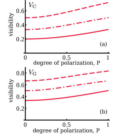
Figure 4: Comparison of the maximum visibility according to the definition by (a) Cao et al. [Eq. (22)] and (b) Gatti et al. [Eq. (24)]. The solid lines correspond to the double-intensity case [Eqs. (25) and (26)], the dashed lines [Eqs. (27) and (28)] and dash-dotted lines [Eqs. (29) and (30)] are for the general and specific triple-intensity setups, respectively.

Triple-intensity setup with one object arm

Lastly, we examine the visibility related to the specific arrangement in Fig. 2(b) which has the normalized output of Eq. (21). As shown in Sec. 2.4, in contrast to the general triple-intensity case, the normalized correlation between the first two arms in this setup is equal to unity ($|\hat{\gamma}^{12}|=1$) and it does not contribute to the image formation. For the remaining correlation parameters we have $|\hat{\gamma}^{13}|=|\hat{\gamma}^{23}|$, $|\hat{\gamma}^{13}|_{\mathrm{min}}=0$, and $|\hat{\gamma}^{13}|_{\mathrm{max}}=1$. Using these, the visibilities according to Eqs. (22) and (24) become

$$V_{\mathrm{C}}^{(3)} =\frac{5P^{2}+3}{7P^{2}+9},$$ (29)

$$V_{\mathrm{G}}^{(3)} =\frac{5P^{2}+3}{6P^{2}+4}.$$ (30)

Equations (29) and (30) are illustrated with the dash-dotted lines in Figs. 4(a) and 4(b). The visibility of the specific triple-intensity ghost-imaging setup behaves similarly to that of the two previous cases we considered above as the DoP is varied. It is smaller than the visibility in the general triple-intensity case but larger than in double-intensity ghost imaging, for all $P$.

All the visibilities improve with the increase of the DoP. This is caused by the fact that while the backgrounds are independent or weakly dependent on $P$, the correlation terms (which contain the image) show a stronger polarization dependence, as is evidenced for instance by Eqs. (13), (19), and (21)]. For each $P$, the visibility in a given arrangement is proportional to the relative abundance of the correlation-term contributions over the background.

4 Signal-to-noise ratio

The visibility is a measure of the (relative) difference between the light ($g_{\mathrm{max}}^{(N)}$) and dark ($g_{\mathrm{min}}^{(N)}$) areas of the image. However, it contains no information about the noise, i.e., the strength of the intensity fluctuations within the image. We have assumed the source to exhibit electric field-vector fluctuations obeying Gaussian statistics. For such a source, $\langle(\Delta I)^{2}\rangle/\langle I\rangle^{2}=(P^{2}+1)/2$, showing that the higher $P$, the larger are the intensity fluctuations in relation to the mean value [31, 39]. Hence the source noise level grows as $P$ increases. The fluctuations are at their minimum $\langle(\Delta I)^{2}\rangle=\langle I\rangle^{2}/2$ when $P=0$, indicating that the noise is comparable to the signal at the source. The source fluctuations will produce a certain amount of noise to the outputs, which we calculate for both double- and triple-intensity ghost imaging. Other sources of noise, such as those in the optical system or the detection, are not taken into account.

In $N$th-order ghost imaging, the quantity $I_{1}\cdots I_{N}$ is the fluctuating signal. Its variance is $\mathrm{var}\left(I_{1}\cdots I_{N}\right)\equiv\bigl{\langle}\left(I_{1}\cdots I_{N}-\left\langle I_{1}\cdots I_{N}\right\rangle\right)^{2}\bigr{\rangle}$ and the related noise is the square root of the variance (or the standard deviation), i.e.,

$$\mathrm{noise}\left(I_{1}\cdots I_{N}\right)=\sqrt{\left\langle I_{1}^{2}\cdots I_{N}^{2}\right\rangle-\left\langle I_{1}\cdots I_{N}\right\rangle^{2}}.$$ (31)

This is the root-mean-square (rms) of the deviation from the mean signal and it is always non-zero for Gaussian statistics. We define the signal-to-noise ratio (SNR) as

$$\mathrm{SNR}^{(N)}\equiv\frac{\left\langle I_{1}\cdots I_{N}\right\rangle}{\mathrm{noise}\left(I_{1}\cdots I_{N}\right)},$$ (32)

i.e., the average signal divided by the associated rms noise.

The transparent parts of the object lead to bright areas in the ghost image with the normalized average signal $g_{\mathrm{max}}$ and the average noise $\mathrm{rms}_{\mathrm{max}}$, as is illustrated in Fig. 3. The maximum signal is obtained when the correlation parameters in Eqs. (13), (19), and (21) take on their maximum values. The SNR related to the bright areas is denoted by $\mathrm{SNR}[g_{\mathrm{max}}^{(N)}]$. On the other hand, the opaque parts of the object lead to dark image areas, and these are characterized by $g_{\mathrm{min}}$ and $\mathrm{rms}_{\mathrm{min}}$ in Fig. 3. The signals for the dark areas are attained when the correlation parameters reach their minima, and the related SNR is denoted by $\mathrm{SNR}[g_{\mathrm{min}}^{(N)}]$. In addition to the SNRs of the bright and dark areas, we examine the minimum and maximum SNRs within the ghost image, denoted by $\mathrm{SNR}_{\mathrm{min}}^{(N)}$ and $\mathrm{SNR}_{\mathrm{max}}^{(N)}$, respectively. It can happen, for example, that the SNR maximum is obtained when the signal achieves its minimum (i.e., $\mathrm{SNR}_{\mathrm{max}}^{(N)}\approx\mathrm{SNR}[g_{\mathrm{min}}^{(N)}]$).

For later use it is convenient, in view of Eq. (31), to introduce the notation

$$\tilde{g}^{(2N)}\equiv\left\langle I_{1}^{2}\cdots I_{N}^{2}\right\rangle/\left\langle I_{1}\right\rangle^{2}\cdots\left\langle I_{N}\right\rangle^{2}$$ (33)

for the $2N$th-order ICF of $N$ different pairs of intensities. The SNR can be written as

$$\mathrm{SNR}^{(N)}=\frac{g^{(N)}}{\sqrt{\tilde{g}^{(2N)}-\left[g^{(N)}\right]^{2}}}$$ (34)

with this notation.

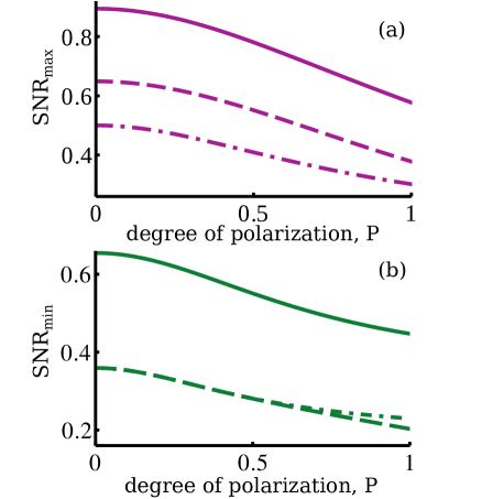
Figure 5: Dependence of the double- and triple-intensity SNRs on the degree of polarization. The solid lines correspond to the extremal SNRs of the second-order ghost-imaging setups shown in Fig. 1. The dashed lines depict the maximum and minimum SNRs of the general third-order correlation imaging arrangement [Fig. 2(a)], while the dash-dotted lines correspond to the extremal SNR values in the specific triple-intensity ghost-imaging setup [Fig. 2(b)]. The maximum SNRs are plotted in purple and the minimum SNRs in green.

4.1 SNR in double-intensity imaging

In Sec. 2 we calculated the second- and third-order ICFs. To find the SNR in the double-intensity case we also need the fourth-order ICF $\left\langle I_{1}^{2}I_{2}^{2}\right\rangle$ or its normalized version $\tilde{g}^{(4)}$. Since it is straightforward but tedious, the computation of the fourth- and higher-order intensity correlations is presented in Appendix C. For a uniformly polarized source and polarization-independent arms, an exact expression for the SNR as a function of the normalized correlation $|\hat{\gamma}^{12}|$ and the degree of polarization $P$ is obtained by inserting Eqs. (13) and (C.4) into the definition given in Eq. (34). From this expression we get the SNR in the dark ($|\hat{\gamma}^{12}|=0$) and light ($|\hat{\gamma}^{12}|=1$) areas of the image. The double-intensity SNR decreases monotonically as a function of $|\hat{\gamma}^{12}|$, so it stays within the range

$$\frac{P^{2}+3}{\sqrt{5P^{4}+54P^{2}+21}}\leq\mathrm{SNR}^{(2)}\leq\frac{2}{\sqrt{P^{4}+6P^{2}+5}},$$ (35)

where the upper limit corresponds to the dark areas and the lower limit to bright areas. Thus, for double-intensity ghost imaging we have $\mathrm{SNR}_{\mathrm{max}}^{(2)}=\mathrm{SNR}[g_{\mathrm{min}}^{(2)}]$ and $\mathrm{SNR}_{\mathrm{min}}^{(2)}=\mathrm{SNR}[g_{\mathrm{max}}^{(2)}]$, which are shown with the solid lines in Figs. 5(a) and 5(b), respectively. The SNR is restricted in between these limits in the absence of other sources of noise. As opposed to the visibility, the SNR decreases as a function of the DoP. The mathematical reason for the SNR reduction with both the correlation parameter $|\hat{\gamma}^{12}|$ and the degree of polarization $P$ is that, although the signal increases with both $|\hat{\gamma}^{12}|$ and $P$, the level of noise grows proportionally more due to the stronger dependence of the higher-order intensity correlations on $|\hat{\gamma}^{12}|$ and $P$ [cf. Eqs. (13) and (C.4)]. Physically this is explained as follows: when $P$ increases, the source noise grows as discussed above, and when $|\hat{\gamma}^{12}|$ increases, the random output signals become more correlated and hence the fluctuations of their product grow.

4.2 SNR in triple-intensity imaging

Referring to the general triple-intensity ghost-imaging setup of Fig. 2(a), we can obtain the associated SNR

$$\mathrm{SNR}^{(3)}=\frac{g^{(3)}}{\sqrt{\tilde{g}^{(6)}-\left[g^{(3)}\right]^{2}}}$$ (36)

as a function of the magnitudes of the correlations between any two arms $|\hat{\gamma}^{\alpha\beta}|$ ($\alpha,\beta\in\{1,2,3\}$, $\alpha\neq\beta$), the phase difference between the arms $\Delta\phi_{123}$, and the degree of polarization $P$, using Eqs. (19) and (C.5).

First, we find the maximum and minimum signal-to-noise ratios $\mathrm{SNR}_{\mathrm{max}}^{(3)}$ and $\mathrm{SNR}_{\mathrm{min}}^{(3)}$ of the ghost image for each degree of polarization $P$. This is done computationally by maximizing and minimizing $\mathrm{SNR}^{(3)}$ from Eq. (36) at each $P$ within the parameter ranges $0\leq|\hat{\gamma}^{\alpha\beta}|\leq 1$ and $-1\leq\cos(\Delta\phi_{123})\leq 1$. Next the SNRs in the dark and bright areas of the image, $\mathrm{SNR}[g_{\mathrm{max}}^{(3)}]$ and $\mathrm{SNR}[g_{\mathrm{min}}^{(3)}]$, are obtained with the assumptions $|\hat{\gamma}^{\alpha\beta}|_{\mathrm{min}}=0$ and $|\hat{\gamma}^{\alpha\beta}|_{\mathrm{max}}=1$ and $\cos(\Delta\phi_{123})=1$, respectively. As in double-intensity correlation imaging, the dark regions of the image are found to have the maximum possible SNR, i.e., $\mathrm{SNR}[g_{\mathrm{min}}^{(3)}]=\mathrm{SNR}_{\mathrm{max}}^{(3)}$, shown by the dashed line in Fig. 5(a). However, in the general case the SNR related to the light regions ($\mathrm{SNR}[g_{\mathrm{max}}^{(3)}]$) is slightly higher than $\mathrm{SNR}_{\mathrm{min}}^{(3)}$, illustrated by the dashed line in Fig. 5(b). In fact, $\mathrm{SNR}[g_{\mathrm{max}}^{(3)}]$ of the general case equals $\mathrm{SNR}_{\mathrm{min}}^{(3)}$ of the specific case (discussed below), shown with the dash-dotted line in the same figure.

The decrease of $\mathrm{SNR}^{(3)}$ when the correlation parameters and the DoP become larger is due to increased noise, as discussed in connection with the double-intensity case. Physically, $\mathrm{SNR}^{(3)}$ is smaller than $\mathrm{SNR}^{(2)}$ since the product of three partially correlated signals is noisier than the product of two such signals.

Triple-intensity imaging with one object arm

The SNR for the specific ghost-imaging setup of Fig. 2(b) is obtained by inserting Eqs. (21) and (C.6) into Eq. (36). Similarly to the second-order case, the SNR decreases monotonically as a function of $|\hat{\gamma}^{13}|$, and thus its maximum and minimum values correspond to the SNR in the dark ($|\hat{\gamma}^{13}|=0$) and light ($|\hat{\gamma}^{13}|=1$) regions of the image, respectively. The SNR extrema are depicted in Fig. 5 by dash-dotted lines. We also found that the SNR in the bright areas of the specific ghost-imaging setup is the same as that of the general triple-intensity correlation imaging case, while the SNR in the dark areas of the specific setup is lower than that of the general case.

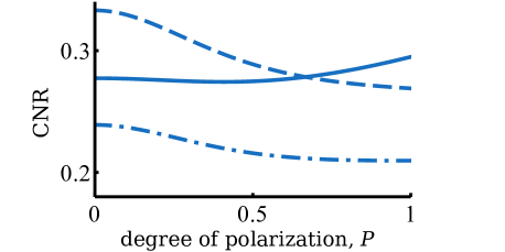
Figure 6: Dependence of the CNR on the degree of polarization. The solid line is for the double-intensity case [Eq. (39)], while the dashed and dash-dotted lines correspond to the CNRs of the triple-intensity cases related to Fig. 2(a) [Eq. (41)] and Fig. 2(b) [Eq. (42)], respectively.

5 Contrast-to-noise ratio

The visibility measures the image contrast and the SNR assesses the noise in various parts of the ghost image. To study the contrast compared to the overall noise in the image we consider a third quality parameter, namely the contrast-to-noise ratio (CNR). It is defined as [22, 27]

$$\mathrm{CNR}^{(N)}\equiv\frac{\left\langle I_{1}\cdots I_{N}\right\rangle_{\mathrm{max}}-\left\langle I_{1}\cdots I_{N}\right\rangle_{\mathrm{min}}}{\sqrt{\frac{1}{2}\left[\mathrm{noise}_{\mathrm{max}}^{2}\left(I_{1}\cdots I_{N}\right)+\mathrm{noise}_{\mathrm{min}}^{2}\left(I_{1}\cdots I_{N}\right)\right]}}.$$ (37)

Referring to Fig. 3, we see that the numerator in Eq. (37) is related to the difference between the average signal in the bright and dark areas of the image and the denominator is the root-mean-squared average of the corresponding noises.

5.1 CNR in double-intensity imaging

The CNR of double-intensity ghost imaging becomes

$$\mathrm{CNR}^{(2)}=\frac{g_{\mathrm{max}}^{(2)}-g_{\mathrm{min}}^{(2)}}{\sqrt{\frac{1}{2}\left\{\tilde{g}_{\mathrm{max}}^{(4)}-\left[g_{\mathrm{max}}^{(2)}\right]^{2}+\tilde{g}_{\mathrm{min}}^{(4)}-\left[g_{\mathrm{min}}^{(2)}\right]^{2}\right\}}},$$ (38)

where we have first substituted from Eq. (31) and then normalized all the intensity correlation functions. Using the limits $|\hat{\gamma}^{12}|{}_{\mathrm{min}}=0$ and $|\hat{\gamma}^{12}|{}_{\mathrm{max}}=1$ for the normalized ICFs given in Eqs. (13) and (C.4), we obtain the expression

$$\mathrm{CNR}^{(2)} =\frac{P^{2}+1}{\sqrt{3P^{4}+30P^{2}+13}}.$$ (39)

For fully polarized light the CNR achieves its maximum, $\mathrm{CNR}_{\mathrm{max}}^{(2)}=\sqrt{2/23}\approx 0.29$. The CNR as a function of $P$ is represented with the solid line in Fig. 6. It is almost constant with a slight rise for higher degrees of polarization.

5.2 CNR in triple-intensity imaging

The triple intensity CNR can be obtained analogously to the second-order case from Eq. (37) and it is

$$\mathrm{CNR}^{(3)}=\frac{g_{\mathrm{max}}^{(3)}-g_{\mathrm{min}}^{(3)}}{\sqrt{\frac{1}{2}\left\{\tilde{g}_{\mathrm{max}}^{(6)}-\left[g_{\mathrm{max}}^{(3)}\right]^{2}+\tilde{g}_{\mathrm{min}}^{(6)}-\left[g_{\mathrm{min}}^{(3)}\right]^{2}\right\}}}.$$ (40)

For the general triple-intensity imaging case [Fig. 2(a)], the normalized ICFs can be retrieved from Eqs. (19) and (C.5). Then, inserting $\cos(\Delta\phi_{123})=1$ and $|\hat{\gamma}^{\alpha\beta}|{}_{\mathrm{max}}=1$ for $g_{\mathrm{max}}^{(3)}$ and $\tilde{g}_{\mathrm{max}}^{(6)}$, and $|\hat{\gamma}^{\alpha\beta}|{}_{\mathrm{min}}=0$ for $g_{\mathrm{min}}^{(3)}$ and $\tilde{g}_{\mathrm{min}}^{(6)}$, with ($\alpha,\beta\in\{1,2,3\}$, $\alpha\neq\beta$), the triple-intensity CNR with respect to the DoP is

$$\mathrm{CNR}^{(3)} =\frac{12P^{2}+8}{\sqrt{91P^{6}+1827P^{4}+3033P^{2}+577}}.$$ (41)

Equation (41) is shown with the dashed line in Fig. 6. For weakly polarized light the improved visibility in third-order correlation imaging leads to CNR values that are slightly higher as compared to the second-order case. For strongly polarized light the triple-intensity CNR falls below $\mathrm{CNR}^{(2)}$ due to the increased noise. The maximum triple-intensity CNR is obtained with completely unpolarized light and it is $\mathrm{CNR}_{\mathrm{max}}^{(3)}=8/\sqrt{577}\approx 0.33$.

Triple-intensity setup with one object arm

As for the general third-order setup, the CNR of the ghost imaging apparatus with two reference arms and one arm containing the object, depicted in Fig. 2(b), is given by Eq. (40). Inserting Eqs. (21) and (C.6) related to the present setup, the CNR becomes

$$\mathrm{CNR}^{(3)} =\frac{\sqrt{2}\left(5P^{2}+3\right)}{\sqrt{48P^{6}+947P^{4}+1602P^{2}+315}},$$ (42)

where we have used the extrema $|\hat{\gamma}^{13}|_{\mathrm{min}}=0$ and $|\hat{\gamma}^{13}|_{\mathrm{max}}=1$ for the correlation between the reference arms and the test arm. Equation (42) is shown in Fig. 6 with the dash-dotted line. It behaves otherwise similarly to the general triple-intensity case [Eq. (41)] but is smaller for all $P$. This is because the contrast is lower (Fig. 4) and the mean noise is slightly higher (Fig. 5) for the specific setup than for the general case. The maximum CNR is $\mathrm{CNR}_{\mathrm{max}}^{(3)}=\sqrt{2/35}\approx 0.24$, valid for completely unpolarized light.

6 Summary and conclusions

We have taken into account the electromagnetic nature of light and studied the influence the degree of polarization (DoP) has on the performance of double- and triple-intensity correlation-imaging arrangements. The illumination was a partially polarized, spatially incoherent beam of light obeying Gaussian field statistics. Both in the double- and triple-intensity setups a general intensity-correlation-imaging system and a specific ghost-imaging arrangement were considered. In all cases the image was assessed in terms of three different quality parameters, namely the visibility (contrast) and the signal-to-noise (SNR) and contrast-to-noise (CNR) ratios.

We found that in all setups the image visibility improves when the degree of polarization increases and it is higher in third-order imaging than in the second-order case. In contrast, the SNR was found to decrease with increasing degree of polarization as the source noise grows with the DoP. In addition, the SNR is lower for third-order imaging than for second-order imaging since in the triple-intensity case the image is created by a product of a larger number of noisy output signals. The CNR stays approximately the same as a function of the DoP, although it does go down slightly for the third-order imaging setups. If the CNR is considered as the most important quality parameter, as many authors do, then our results put into question the earlier suggestions of improved image quality with increased imaging order and DoP. Our results imply that increasing the imaging order might even be harmful and, on the other hand, changing the DoP does not have much of an effect and hence no polarizers are necessarily needed in experiments.

The SNR and CNR in ghost imaging with Gaussian light generally assume low values due to the noisy source. The impediments of the source noise are further enhanced by the correlations and the number of the output fields. The quality parameters studied in this work do not depend on the state of polarization of the polarized part of the illuminations, since the arms in the ghost-imaging setups were taken to be polarization independent.

Appendix A Traces of $\mathbf{J}_{0}$

In terms of the eigenvalues $J_{1}$ and $J_{2}$ of $\mathbf{J}_{0}$ we have

$$\mathrm{tr}\left(\mathbf{J}_{0}^{n}\right) =J_{1}^{n}+J_{2}^{n} =J_{1}^{n}(1+x^{n}),$$ (A.1)

$$\left(\mathrm{tr}\mathbf{J}_{0}\right)^{n} =\left(J_{1}+J_{2}\right)^{n} =J_{1}^{n}(1+x)^{n},$$ (A.2)

where $x\equiv J_{2}/J_{1}\leq 1$. Using the degree of polarization [Eq. (2)] we can write

$$x=\frac{1-P}{1+P}.$$ (A.3)

This implies that

$$\frac{\mathrm{tr}\left(\mathbf{J}_{0}^{n}\right)}{\left(\mathrm{tr}\mathbf{J}_{0}\right)^{n}}=\frac{\left(1+P\right)^{n}+\left(1-P\right)^{n}}{2^{n}},$$ (A.4)

where we used Eqs. (A.1)–(A.3).

Appendix B Partially coherent source

To calculate a value for the correlation coefficient $\hat{\gamma}^{12}$ in Sec. 2.4 we express the source coherence function as $\mathbf{\Gamma}_{0}(\mathbf{r}_{1}^{\prime},\mathbf{r}_{2}^{\prime})=\mathbf{J}_{0}\gamma(\mathbf{r}_{2}^{\prime}-\mathbf{r}_{1}^{\prime})$, where $\gamma(\mathbf{r}_{2}^{\prime}-\mathbf{r}_{1}^{\prime})$ is a normalized coherence function with the property $\gamma(\mathbf{0})=1$. With the change of variables $\mathbf{r}=\mathbf{r}_{2}^{\prime}-\mathbf{r}_{1}^{\prime}$ and $\mathbf{R}=\left(\mathbf{r}_{1}^{\prime}+\mathbf{r}_{2}^{\prime}\right)/2$, Eq. (11) becomes

$$\hat{\Gamma}^{\alpha\beta}=\iint\gamma(\mathbf{r})K_{\alpha}^{*}(\mathbf{r}_{\alpha},\mathbf{R}-\frac{\mathbf{r}}{2})K_{\beta}(\mathbf{r}_{\beta},\mathbf{R}+\frac{\mathbf{r}}{2})\mathrm{d}\mathbf{r}\mathrm{d}\mathbf{R}.$$ (B.1)

Inserting the kernels from Eq. (14) corresponding to the reference arms, the integral with respect to $\mathbf{R}$ is proportional to $\delta\left[\left(\mathbf{r}_{\beta}-\mathbf{r}_{\alpha}\right)/\left(1-z_{b}/f\right)-\mathbf{r}\right]$ and we find that

$$\hat{\Gamma}^{\alpha\beta} =\frac{1}{\left|1-z_{b}/f\right|^{2}}\gamma\left(\frac{\mathbf{r}_{\beta}-\mathbf{r}_{\alpha}}{1-z_{b}/f}\right)$$

$$\times\exp\left\{\frac{ik}{2\zeta}\left[\left(\mathbf{r}_{\beta}^{2}-\mathbf{r}_{\alpha}^{2}\right)\left(1-\frac{z_{a}}{f}\right)-\frac{\left(\mathbf{r}_{\beta}-\mathbf{r}_{\alpha}\right)^{2}}{1-z_{b}/f}\right]\right\}.$$ (B.2)

When $\mathbf{r}_{1}=\mathbf{r}_{2}$ the normalized correlation takes on the value $\hat{\gamma}^{12}=\hat{\Gamma}^{12}/\sqrt{\hat{\Gamma}^{11}\hat{\Gamma}^{22}}=1$.

Appendix C Fourth- and higher-order intensity correlations

To calculate the noise for the SNR and CNR in the double-intensity case we need to know the fourth-order ICF $\langle I_{1}^{2}I_{2}^{2}\rangle$, and for triple-intensity imaging we need the sixth-order ICF $\langle I_{1}^{2}I_{2}^{2}I_{3}^{2}\rangle$. These are obtained from Eqs. (5) and (6) with the help of the matrix property

$$\sum_{n_{1},\ldots,n_{m}\in\{x,y\}}A_{n_{1}n_{2}}^{1}A_{n_{2}n_{3}}^{2}\cdots A_{n_{m}n_{1}}^{m}=\mathrm{tr}(A^{1}\cdots A^{m}),$$ (C.1)

where

$$A^{i}=\left[\begin{array}[]{cc}A_{xx}^{i}&A_{xy}^{i}\\ A_{yx}^{i}&A_{yy}^{i}\end{array}\right]$$ (C.2)

are arbitrary $2\times 2$ matrices for all $i\in\{1,\ldots,m\}$. Therefore, the fourth-order ICF takes on the form

$$\left\langle I_{1}^{2}I_{2}^{2}\right\rangle =\left[\mathrm{tr}\mathbf{\Gamma}^{11}\right]^{2}\left[\mathrm{tr}\mathbf{\Gamma}^{22}\right]^{2}+\mathrm{tr}(\mathbf{\Gamma}^{11}\mathbf{\Gamma}^{11})\left[\mathrm{tr}\mathbf{\Gamma}^{22}\right]^{2}$$

$$+\left[\mathrm{tr}\mathbf{\Gamma}^{11}\right]^{2}\mathrm{tr}(\mathbf{\Gamma}^{22}\mathbf{\Gamma}^{22})+\mathrm{tr}(\mathbf{\Gamma}^{11}\mathbf{\Gamma}^{11})\mathrm{tr}(\mathbf{\Gamma}^{22}\mathbf{\Gamma}^{22})$$

$$+2\left[\mathrm{tr}(\mathbf{\Gamma}^{12}\mathbf{\Gamma}^{21})\right]^{2}+2\mathrm{tr}(\mathbf{\Gamma}^{12}\mathbf{\Gamma}^{21}\mathbf{\Gamma}^{12}\mathbf{\Gamma}^{21})$$

$$+4\mathrm{tr}\mathbf{\Gamma}^{11}\mathrm{tr}\mathbf{\Gamma}^{22}\mathrm{tr}(\mathbf{\Gamma}^{12}\mathbf{\Gamma}^{21})+4\mathrm{tr}(\mathbf{\Gamma}^{11}\mathbf{\Gamma}^{12}\mathbf{\Gamma}^{21})\mathrm{tr}\mathbf{\Gamma}^{22}$$

$$+4\mathrm{tr}\mathbf{\Gamma}^{11}\mathrm{tr}(\mathbf{\Gamma}^{12}\mathbf{\Gamma}^{22}\mathbf{\Gamma}^{21})+4\mathrm{tr}(\mathbf{\Gamma}^{11}\mathbf{\Gamma}^{12}\mathbf{\Gamma}^{22}\mathbf{\Gamma}^{21}),$$ (C.3)

where $\mathbf{\Gamma}^{\alpha\beta}$, with $\alpha,\beta\in(1,2)$, are given by Eq. (7). When the source is uniformly polarized and the arms do not depend on polarization, the normalized version of Eq. (C.3) becomes

$$\tilde{g}^{(4)} =\frac{P^{4}+6P^{2}+9}{4}+\frac{P^{4}+22P^{2}+9}{2}\bigl{|}\hat{\gamma}^{12}\bigr{|}^{2}$$

$$+\frac{3P^{4}+10P^{2}+3}{4}\bigl{|}\hat{\gamma}^{12}\bigr{|}^{4},$$ (C.4)

where Eqs. (10) and (A.4) were used. Likewise, on normalization and applying Eqs. (10) and (A.4), the sixth-order ICF associated with the general case of Fig. 2(a) assumes the form

$$\tilde{g}^{(6)} =\frac{1}{8}\bigl{\{}(P^{6}+9P^{4}+27P^{2}+27)$$

$$+2(P^{6}+25P^{4}+75P^{2}+27)(\left|\hat{\gamma}_{12}\right|^{2}+\left|\hat{\gamma}_{23}\right|^{2}+\left|\hat{\gamma}_{13}\right|^{2})$$

$$+(3P^{6}+19P^{4}+33P^{2}+9)(\left|\hat{\gamma}_{12}\right|^{4}+\left|\hat{\gamma}_{13}\right|^{4}+\left|\hat{\gamma}_{23}\right|^{4})$$

$$+2(P^{6}+89P^{4}+139P^{2}+27)$$

$$\times(\left|\hat{\gamma}_{12}\right|^{2}\left|\hat{\gamma}_{23}\right|^{2}+\left|\hat{\gamma}_{12}\right|^{2}\left|\hat{\gamma}_{13}\right|^{2}+\left|\hat{\gamma}_{13}\right|^{2}\left|\hat{\gamma}_{23}\right|^{2})$$

$$+2(P^{6}+33P^{4}+27P^{2}+3)\left|\hat{\gamma}_{12}\right|^{2}\left|\hat{\gamma}_{23}\right|^{2}\left|\hat{\gamma}_{31}\right|^{2}\cos^{2}(\Delta\phi_{123})$$

$$+4(3P^{6}+51P^{4}+65P^{2}+9)$$

$$\times(\left|\hat{\gamma}_{12}\right|^{2}+\left|\hat{\gamma}_{23}\right|^{2}+\left|\hat{\gamma}_{13}\right|^{2})\left|\hat{\gamma}_{12}\right|\left|\hat{\gamma}_{23}\right|\left|\hat{\gamma}_{31}\right|\cos(\Delta\phi_{123})$$

$$+4(P^{6}+57P^{4}+171P^{2}+27)\left|\hat{\gamma}_{12}\right|\left|\hat{\gamma}_{23}\right|\left|\hat{\gamma}_{31}\right|\cos(\Delta\phi_{123})$$

$$+2(13P^{6}+117P^{4}+111P^{2}+15)\left|\hat{\gamma}_{12}\right|^{2}\left|\hat{\gamma}_{23}\right|^{2}\left|\hat{\gamma}_{13}\right|^{2}\bigr{\}}.$$ (C.5)

For the specific setup of Fig. 2(b) we have $|\hat{\gamma}^{12}|=1$, $|\hat{\gamma}^{13}|=|\hat{\gamma}^{23}|$, and $\Delta\phi_{123}=0$, in which case Eq. (C.5) reduces to

$$\tilde{g}^{(6)} =\frac{3P^{6}+39P^{4}+105P^{2}+45}{4}$$

$$+(3P^{6}+111P^{4}+225P^{2}+45)\left|\hat{\gamma}^{13}\right|^{2}$$

$$+\frac{15P^{6}+231P^{4}+285P^{2}+45}{2}\left|\hat{\gamma}^{13}\right|^{4}.$$ (C.6)

The generation of the sixth-order ICF and its subsequent simplification were handled with symbolic computational software.

References

- [1] A. Gatti, E. Brambilla, and L. Lugiato, “Quantum imaging,” in Progress in Optics vol. 51, E. Wolf, ed. (Elsevier, 2008), pp. 251–348.
- [2] B. I. Erkmen and J. H. Shapiro, “Ghost imaging: from quantum to classical to computational,” Adv. Opt. Photon. 2, 405–450 (2010).
- [3] T. Pittman, Y. Shih, D. Strekalov, and A. Sergienko, “Optical imaging by means of two-photon quantum entanglement,” Phys. Rev. A 52, R3429 (1995).
- [4] D. Strekalov, A. Sergienko, D. Klyshko, and Y. Shih, “Observation of two-photon “ghost” interference and diffraction,” Phys. Rev. Lett. 74, 3600 (1995).
- [5] R. Bennink, S. Bentley, and R. Boyd, “Two-photon coincidence imaging with a classical source,” Phys. Rev. Lett. 89, 113601 (2002).
- [6] A. Gatti, E. Brambilla, M. Bache, and L. Lugiato, “Correlated imaging, quantum and classical,” Phys. Rev. A 70, 013802 (2004).
- [7] A. Valencia, G. Scarcelli, M. D’Angelo, and Y. Shih, “Two-photon imaging with thermal light,” Phys. Rev. Lett. 94, 063601 (2005).
- [8] V. Torres-Company, H. Lajunen, J. Lancis, and A. T. Friberg, “Ghost interference with classical partially coherent light pulses,” Phys. Rev. A 77, 043811 (2008).
- [9] T. Setälä, T. Shirai, and A. T. Friberg, “Fractional Fourier transform in temporal ghost imaging with classical light,” Phys. Rev. A 82, 043813 (2010).
- [10] T. Shirai, T. Setälä, and A. T. Friberg, “Temporal ghost imaging with classical non-stationary pulsed light,” J. Opt. Soc. Am. B 27, 2549–2555 (2010).
- [11] T. Shirai, T. Setälä, and A. Friberg, “Ghost imaging of phase objects with classical incoherent light,” Phys. Rev. A 84, 041801(R) (2011).
- [12] J. Cheng, “Ghost imaging through turbulent atmosphere,” Opt. Express 17, 7916–7921 (2009).
- [13] C. Li, T. Wang, J. Pu, W. Zhu, and R. Rao, “Ghost imaging with partially coherent light radiation through turbulent atmosphere,” Appl. Phys. B 99, 599–604 (2010).
- [14] P. Zhang, W. Gong, X. Shen, and S. Han, “Correlated imaging through atmospheric turbulence,” Phys. Rev. A 82, 033817 (2010).
- [15] K. W. C. Chan, D. S. Simon, A. V. Sergienko, N. D. Hardy, J. H. Shapiro, P. B. Dixon, G. A. Howland, J. C. Howell, J. H. Eberly, M. N. O’Sullivan, B. Rodenburg, and R. W. Boyd, “Theoretical analysis of quantum ghost imaging through turbulence,” Phys. Rev. A 84, 043807 (2011).
- [16] T. Shirai, H. Kellock, T. Setälä, and A. T. Friberg, “Imaging through an aberrating medium with classical ghost diffraction,” J. Opt. Soc. Am. A 29, 1288–1292 (2012).
- [17] A. Gatti, E. Brambilla, M. Bache, and L. Lugiato, “Ghost imaging with thermal light: Comparing entanglement and classical correlation,” Phys. Rev. Lett. 93, 093602 (2004).
- [18] F. Ferri, D. Magatti, A. Gatti, M. Bache, E. Brambilla, and L. Lugiato, “High-resolution ghost image and ghost diffraction experiments with thermal light,” Phys. Rev. Lett. 94, 183602 (2005).
- [19] A. Gatti, M. Bache, D. Magatti, E. Brambilla, F. Ferri, and L. A. Lugiato, “Coherent imaging with pseudo-thermal incoherent light,” J. Mod. Opt. 53, 739–760 (2006).
- [20] D.-Z. Cao, J. Xiong, S.-H. Zhang, L.-F. Lin, L. Gao, and K. Wang, “Enhancing visibility and resolution in th-order intensity correlation of thermal light,” Appl. Phys. Lett. 92, 201102 (2008).
- [21] H.-G. Li, Y.-T. Zhang, D.-Z. Cao, J. Xiong, and K.-G. Wang, “Third-order ghost interference with thermal light,” Chin. Phys. B 17, 4510–4515 (2008).
- [22] K. W. C. Chan, M. N. O’Sullivan, and R. W. Boyd, “Optimization of thermal ghost imaging: high-order correlations vs. background subtraction,” Opt. Express 18, 5562–5573 (2010).
- [23] F. Ferri, D. Magatti, L. Lugiato, and A. Gatti, “Differential ghost imaging,” Phys. Rev. Lett. 104, 253603 (2010).
- [24] J. H. Shapiro, “Computational ghost imaging,” Phys. Rev. A 78, 061802 (2008).
- [25] Y. Bromberg, O. Katz, and Y. Silberberg, “Ghost imaging with a single detector,” Phys. Rev. A 79, 053840 (2009).
- [26] I. Agafonov, M. Chekhova, T. S. Iskhakov, and L.-A. Wu, “High-visibility intensity interference and ghost imaging with pseudo-thermal light,” J. Mod. Opt. 56, 422–431 (2009).
- [27] G. Brida, M. Chekhova, G. Fornaro, M. Genovese, E. Lopaeva, and I. Berchera, “Systematic analysis of signal-to-noise ratio in bipartite ghost imaging with classical and quantum light,” Phys. Rev. A 83, 063807 (2011).
- [28] H.-C. Liu, D.-S. Guan, L. Li, S.-H. Zhang, and J. Xiong, “The impact of light polarization on imaging visibility of th-order intensity correlation with thermal light,” Opt. Commun. 283, 405–408 (2010).
- [29] Z. Tong, Y. Cai, and O. Korotkova, “Ghost imaging with electromagnetic stochastic beams,” Opt. Commun. 283, 3838–3845 (2010).
- [30] T. Shirai, H. Kellock, T. Setälä, and A. T. Friberg, “Visibility in ghost imaging with classical partially polarized electromagnetic beams,” Opt. Lett. 36, 2880–2882 (2011).
- [31] L. Mandel and E. Wolf, Optical Coherence and Quantum Optics (Cambridge University Press, 1995).
- [32] J. W. Goodman, Statistical Optics (Wiley, 1985).
- [33] J. W. Goodman, Introduction to Fourier Optics (McGraw-Hill, 1996), 2nd ed.
- [34] D.-Z. Cao, J. Xiong, and K. Wang, “Geometrical optics in correlated imaging systems,” Phys. Rev. A 71, 013801 (2005).
- [35] Y. Cai and S.-Y. Zhu, “Ghost imaging with incoherent and partially coherent light radiation,” Phys. Rev. E 71, 056607 (2005).
- [36] K. W. C. Chan, M. N. O’Sullivan, and R. W. Boyd, “High-order thermal ghost imaging,” Opt. Lett. 34, 3343–3345 (2009).
- [37] Y.-C. Liu and L.-M. Kuang, “A theoretical scheme of thermal-light ghost imaging by th-order intensity correlation,” (2009). arXiv:0903.5015.
- [38] H. Kellock, T. Setälä, T. Shirai, and A. T. Friberg, “Higher-order ghost imaging with partially polarized classical light,” Proc. SPIE 8171, 81710Q (2011).
- [39] T. Setälä, K. Lindfors, M. Kaivola, J. Tervo, and A. T. Friberg, “Intensity fluctuations and degree of polarization in three-dimensional thermal light fields,” Opt. Lett. 29, 2587–2589 (2004).