Quantum spin models with long-range interactions and tunnelings: A quantum Monte Carlo study.

Abstract

We use a quantum Monte Carlo method to investigate various classes of 2D spin models with long-range interactions at low temperatures. In particular, we study a dipolar XXZ model with $U(1)$ symmetry that appears as a hard-core boson limit of an extended Hubbard model describing polarized dipolar atoms or molecules in an optical lattice. Tunneling, in such a model, is short-range, whereas density-density couplings decay with distance following a cubic power law. We investigate also an XXZ model with long-range couplings of all three spin components - such a model describes a system of ultracold ions in a lattice of microtraps. We describe an approximate phase diagram for such systems at zero and at finite temperature, and compare their properties. In particular, we compare the extent of crystalline, superfluid, and supersolid phases. Our predictions apply directly to current experiments with mesoscopic numbers of polar molecules and trapped ions.

1 Introduction

Quantum simulators, as first proposed by Feynman [1], which are devices built to evolve according to a postulated quantum Hamiltonian and thus “compute” its properties, are one of the hot ideas which may provide a breakthrough in many-body physics. While one must be aware of possible difficulties (see, e.g., [2]), impressive progress has been achieved in recent years in different systems employing cold atoms and molecules, nuclear magnetic resonance, superconducting qubits, and ions. The latter are extremely well controlled and already it has been demonstrated that, indeed, quantum spin systems may be simulated with cold-ion setups [3, 4]. Quantum spin systems on a lattice constitute some of the most relevant cases for quantum simulations as there are many instances where standard numerical techniques to compute their dynamics or even their static behavior fail, especially for two- or three-dimensional systems.

Chronologically the first proposition to use trapped ions to simulate lattice spin models came from Porras and Cirac [5] who derived the effective spin-Hamiltonian for the system ,

$$H=J\sum\limits_{i,j}\frac{1}{|i-j|^{3}}[\cos{\theta}(S_{i}^{z}S_{j}^{z})+\sin{\theta}(S_{i}^{x}S_{j}^{x}+S_{i}^{y}S_{j}^{y})]-\mu\sum\limits_{i}S_{i}^{z},$$ (1)

where $\mu$ is the chemical potential (which in this case acts as an external magnetic field), $J>0$ is the interaction strength, and $S_{i}^{\alpha}$ are the spin operators at site $i$. All the long-ranged interactions fall off with a $1/r^{3}$ dipolar decay, which for the ions is due to the fact that they are both induced by the same mechanism, namely lattice vibrations mediated by the Coulomb force [7]. Hamiltonian (1) is a dipolar XXZ model where the ratio of hopping to dipolar repulsion can be scaled by $\theta$ [8, 9]. Another route to simulate quantum magnetism of dipolar systems, using the rotational structure of the ultracold polar molecules, has been proposed in Refs. [10, 11]. In this case, the XY (or tunneling) term is restricted to nearest neighbors (NN) and only the ZZ (or interaction) term is dipolar.

Precisely this long-range (LR) dipolar character makes this system interesting and challenging. Dipolar interactions introduce new physics to conventional short-range (SR) systems. For example, for soft-core bosons, the system with long-range interactions and short-range tunneling, can – apart from Mott-insulating (MI), superfluid (SF), and crystal phases – host a Haldane-insulating phase [12]. This is characterized by antiferromagnetic (AFM) order between empty sites and sites with double occupancy, with an arbitrarily long string of sites with unit occupancy in between. Another case where dipolar interactions play a crucial role is the appearance of the celebrated supersolid. The extended Bose-Hubbard model (i.e., with NN interactions) with soft-core on-site interactions shows stable supersolidity in one-dimensional (1D) [13] and square lattices [14], where in the 1D case a continuous transition to the supersolid phase occurs, in contrast to the first-order phase transition in two-dimensional (2D) lattices. Long-ranged dipolar interactions on the other hand allow for the appearance of supersolidity even in the hard-core limit [15, 16]. In this limit, dipolar interactions give rise to a large number of metastable states [17, 18] (for a review see [19]). By tuning the direction of the dipoles, incompressible regions like devil’s staircase structures have been predicted in Ref. [20]. While being interesting, long-range interactions make computer simulations of such systems quite difficult. On the other hand, since ions in optical lattices may be extremely well controlled, they form an ideal medium for a quantum simulator.

In our previous paper [8], we considered both the mean-field phase diagram for the system (1) as well as a 1D chain using different quasi-exact techniques, such as density matrix renormalization group (DMRG), and exact diagonalization for small systems. Here, we would like to concentrate on frustration effects on a 2D triangular lattice using a quantum Monte Carlo (QMC) approach.

For the system consisting of spin-half particles (as, e.g., originating from two internal ion states in the Porras–Cirac [7] proposal) the spins can be mapped onto a system of hard-core bosons, using the Holstein–Primakoff transformation, $S_{i}^{z}\rightarrow n_{i}-1/2$, $S_{i}^{+}\rightarrow a_{i}^{{\dagger}}$, and $S_{i}^{-}\rightarrow a_{i}$, where $a_{i}^{{\dagger}}$ $(a_{i})$ are the creation (annihilation) operators of hard-core bosons and $n_{i}$ is the number operator at site $i$. These bosons obey the normal bosonic commutation relationships, $[a,a^{{\dagger}}]=1$, but are constrained to only single filling, $a^{2}=(a^{{\dagger}})^{2}=0$. This is the limit when the on-site repulsion term $U$ goes to infinity in the standard Bose-Hubbard model. In this representation, a spin up particle is represented by a filled site and a spin down particle by an empty site. For convenience, we will mostly use the language of hard-core bosons in this paper.

Before presenting the results for the 2D triangular lattice, let us briefly review the behavior of the system for a 1D chain of bosons as obtained in Ref. [8].

2 Review of the results in one dimension

In order to form some intuition about possible physical effects due to the LR interaction and tunneling, we now discuss briefly the ground-state phase diagram of the Hamiltonian in 1D. For hard-core bosons, which is the topic of this article, the one-dimensional version of the Hamiltonian has been thoroughly investigated in the past [8] (see also [21, 22] for the special cases $\theta=0$ and $\theta=\pi/2$). For reference, we reproduce in Fig. 1 the phase diagrams for the system with dipolar interaction and NN tunneling, as well as the system with both the interaction and the tunneling terms dipolar.

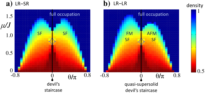
Figure 1: Phase diagram of the 1D system with dipolar interactions and (a) nearest-neighbor tunneling, (b) dipolar tunneling. The phases are labeled according to density matrix renormalization results, while the actual data shown comes from the infinite time evolving block decimation method (with interactions truncated at next-to-nearest-neighbors), both from Ref. [8]. Along the black line, there exists a devil’s staircase of crystal states. At finite tunneling, for (a), these spread into conventional insulating states, while for (b), they form quasi-supersolids. The light blue lines near the center of the plots sketch the crystal lobes at $2/3$-filling. Their cusp-like structure is typical for 1D systems. In 2D, they are expected to be rounded off, similar to Mott-lobes of the Bose–Hubbard model [23]. For nearest-neighbor tunneling, (a), the superfluid (SF) phases can be mapped into one another, while for nearest-neighbor dipolar tunneling, (b), they are distinct on the ferromagnetic (FM, $\theta<0$) and the antiferromagnetic side (AFM, $\theta>0$). Note also that in (b) frustration leads to an asymmetry between $\theta<0$ and $\theta>0$.

At zero tunneling, the ground states are periodic crystals where – to minimize the dipolar interaction energy – occupied sites are as far apart as possible for a given filling factor [21]. For finite 1D systems and very small tunneling such a situation persists as exemplified in [24]. For infinite chains in 1D, every fractional filling factor $n=p/q$ is a stable ground state for a portion of $\mu$ parameter space. The extent in $\mu$ decreases with $q$, since at large distances the dipolar repulsion is weak and thus cannot efficiently stabilize crystals with a large period. This succession of crystal states is termed the devil’s staircase. This name derives from its surprising mathematical properties, challenging naive intuitions about continuity and measure: since all rational fillings are present, it is a continuous function; moreover, its derivative vanishes almost everywhere (i.e., it is non-zero only on a set of measure zero) – and still it is not a constant, but covers a finite range.

At finite tunneling, the crystals spread into lobes similar to the Mott lobes of the Bose–Hubbard model. If the tunneling is only over NNs, these Mott lobes are not sensitive to the sign of the tunneling and they form standard insulating states with diagonal long-range order (LRO) and off-diagonal short-range order (Fig. 1a). For long-range dipolar tunneling, the extent of the lobes is asymmetric under sign change $\theta\to-\theta$: frustration effects stabilize the crystal states for $\theta<0$, while the ferromagnetic (FM) tunneling for $\theta>0$ destabilizes them (Fig. 1b). Moreover, the crystal states acquire off-diagonal correlations which follow the algebraic decay of the dipolar interactions [8]. This coexistence of diagonal and off-diagonal (quasi-)LRO turns the crystal states into (quasi-)supersolids. The occurrence of such phases for hard-core bosons in 1D is truly exceptional, since the systems where it appears consist typically of soft-core bosons [13, 14], or two-dimensional lattices [15]. Furthermore, this 1D quasi-supersolid defies Luttinger-liquid theory, which typically describes 1D systems very well, even in the presence of dipolar interactions [25, 26, 27]. Where Luttinger-liquid theory applies, diagonal and off-diagonal correlations decay algebraically with exponents which are the inverse of one another. Therefore, if the diagonal correlations show LRO, the corresponding exponent is effectively $0$, and the exponent for the off-diagonal correlations is infinite, describing an exponential decay. In our case, this exponent remains finite in the quasi-supersolid phase and the above relationship clearly does not hold.

At even stronger tunneling strengths, the crystal melts and the system is in a SF phase. The LR tunneling and interactions influence the correlation functions at large distances and therefore also modify the character of this phase [8, 22].

These results show that in this system the dipolar interactions considerably modify the quantum-mechanical phase diagram. In higher dimensions, we can expect the influence of long-range interactions to be even stronger, which makes extending these studies to a two-dimensional lattice highly relevant. For example, one can expect that – if quasi-supersolids appear already in 1D – the long-range tunneling has a profound effect on the stability of two-dimensional supersolids, which appear in triangular lattices at the transition between crystal and superfluid phases [13, 28, 29, 30]. Also, the frustration effects already observed in the 1D system should be much more pronounced in the triangular lattice, simply due to the increased number of interactions.

Further, such an analysis is especially relevant at finite temperature. In fact, a recent work scanned the phase diagram of Hamiltonian (1) along the line $\mu=0$ in a square lattice [9]. There, the authors found that above the superfluid on the FM side (i.e., $\theta<0$), the continuous U(1) symmetry of the off-diagonal correlations remains broken even at finite temperatures. Thus, the long-range nature of the tunneling leads to a phase which defies the Mermin–Wagner theorem [31].

For these reasons, we can expect intriguing effects of the long-range tunneling for the two dimensional triangular lattice, to which we turn now.

3 Dipolar hard-core bosons on the triangular lattice

To analyze the system of dipolar bosons on the two dimensional triangular lattice, we employ quantum Monte Carlo (QMC) simulations at a finite but low temperature. Specifically, we study rhombic lattices with periodic boundary conditions and $N=L\times L$ sites, with $L=6..12$. We will in particular thoroughly investigate the Wigner crystal at $2/3$-filling. The triangular lattice is frustrated even with only NN interactions. When any longer ranged interactions are added, this only increases the frustration, which also makes QMC calculations more difficult. Also, in frustrated systems [32] and systems with long-range interactions [18] typically many metastable states appear, making finding the ground state a somewhat difficult task. To avoid complications with the sign problem, caused by negative probabilities in QMC codes, we will take only negative values of $\theta$ under consideration. Note that this sign problem appears only for the long-ranged XY interactions, while the ZZ (Ising-like) interactions are – despite frustration – sign-problem free.

In this study, we compare the Hamiltonian with both long-range interactions and hoppings (LR–LR), with long-ranged dipolar interactions but NN hopping (LR–SR; relevant for polar molecules [33]), as well as with hopping and interactions truncated at NNs (SR–SR; this is the NN XXZ model, relevant to magnetic materials with planar anisotropy in their couplings). Each of these systems will display different crystal, superfluid, and supersolid regions. Comparing these cases will give valuable insight into the influence of the long-range terms.

All the calculations were performed using the worm algorithm of the open source ALPS (Algorithms and Libraries for Physics Simulations) project [34]. This algorithm, first created by N. Prokof’ev, works by sampling world lines in the path integral representation of the partition function in the grand canonical ensemble [35].

3.1 Vanishing tunneling

The first calculation, which creates the motivation for the rest of the paper, is to look at the case of vanishing tunneling and temperature for each system (LR–LR, LR–SR, and SR–SR). Here, similar to the 1D devil’s staircase, at vanishing temperature a series of insulating crystal states is expected to cover the entire range of $\mu/J$. Since we are interested in finite temperature results, we set $T=0.1$ – which should still be low enough to reflect the characteristics of the ground-state phase diagram – and look for plateaus in the density. We distinguish short- and long-ranged ZZ interactions. From Fig. 2, left panel, we can see that the only plateau (besides the completely filled system) that appears is at $\rho=2/3$ (corresponding either to $2/3$ boson filling or in spin terms, a lattice with $2/3$ of the spins oriented up and $1/3$ oriented down) for both short- and long-ranged interactions. Scaling the system size from $L=6$ to $L=12$ causes no change for the short-ranged interactions, and minimal change for the long-ranged ones. The key difference is in the size and position of the short-ranged and the long-ranged plateaus. For short-ranged interactions this plateau is larger and centered around $\mu/J\simeq 1.5$, while the long-ranged interactions have a smaller plateau centered around $\mu/J\simeq 1.85$. The finite width of these plateaus suggests that a $2/3$-filling Wigner crystal persists also for some finite $\theta$. The right panels of Fig. 2 show how the plateau shrinks with increasing temperature, as well for SR interactions (top right panel) as for LR interactions (bottom right panel). In the latter case, in fact, by $T=0.25$ the plateau has completely disappeared. We can also notice that at $T=0.05$ there are signs of some of the other plateaus, most noticably the $3/4$-filling plateau. The rest of the paper will focus on the $2/3$-filling crystal lobes and their properties.

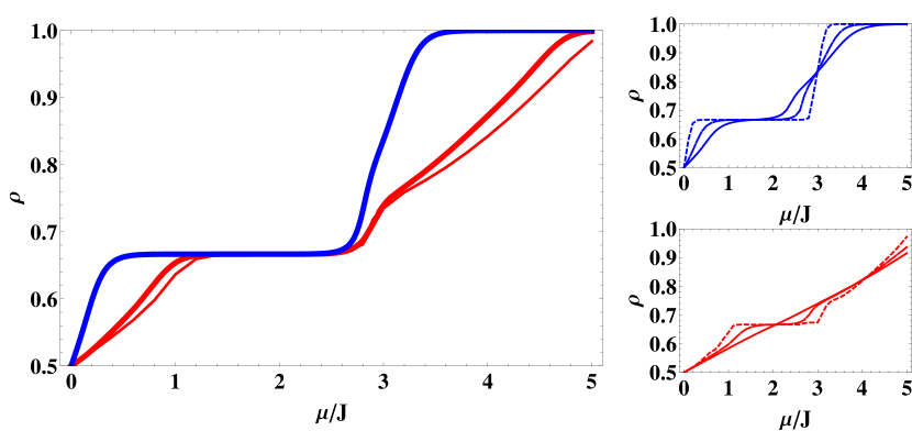
Figure 2: The graph on the left displays $\theta=0$ and $T=0.1$, where the density shows a single plateau for $2/3$-filling. For SR interactions (solid blue line), different curves for $L=6,9,12$coincide, and for LR interactions (solid red: $L=6$, dashed red: $L=9$ and $12$) the size dependence is small. The panels on the right are at fixed $L=12$ and $\theta=0$ for different temperatures $T=0.05,0.15,0.25$ (from dotted to dashed to solid). Both for SR (top right) and LR interactions (bottom right), the $2/3$-filling plateau shrinks as T increases.

3.2 Low-temperature phase diagram at finite tunneling

We now introduce a finite tunneling by choosing $\theta<0$ in our Hamiltonian, and study the properties around the $2/3$-filling crystal. We calculate the density and the superfluid fraction. The superfluidity is measured using the winding numbers calculated from the movement of the worms in the QMC code. In order to get this value the system must have periodic boundary conditions so that the world lines can properly “wind” around the system. The superfluid fraction is

$$\rho_{s}=\frac{\langle W^{2}\rangle}{4\beta},$$ (2)

where $W$ is the winding number fluctuation of the world lines and $\beta$ is the inverse temperature.

Figure 3 shows the results for the boson density of a $L=6$ triangular lattice at $T=0.1$. For all types of interactions we see that as $\theta$ increases in absolute value the $\rho=\frac{2}{3}$ plateau shrinks, because larger $|\theta|$ increases the ratio of hopping to dipolar interactions. This introduces more kinetic energy and the crystal melts into a superfluid. It can be seen for the SR–SR system that the boson density lobe extends to $\theta\simeq-0.36$, while for the LR–SR interactions it ends at $\theta\simeq-0.3$, and finally for LR–LR interactions the lobe is smaller still, only going out to $\theta\simeq-0.2$. The behavior is explained by the fact that the increased amount of interactions cause a quicker melting of the lobe.

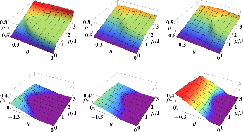
Figure 3: The columns show the $\rho=2/3$ lobes, evidenced by particle density (top row) and the superfluid fraction (bottom row) that arise under varying the ratio, $\theta$, and the chemical potential, $\mu/J$ (data for $L=6$). The left column corresponds to the SR–SR system, the middle one shows the LR–SR system and the right column depicts the lobes for the LR–LR system. Long-ranged dipolar interactions decrease the lobes in $\mu/J$ due to the appearance of devil’s staircase like features, and long-range tunneling decreases the extent of the lobe in $\theta$.

A second major observation is the shift in the position of the lobes. While the short-ranged lobe exists approximately for $0.3<\mu/J<2.7$, the long-ranged lobes lie generally on the interval $1.0<\mu/J<2.8$. For a system like this at $T=0$, one expects the $\rho=\frac{2}{3}$ lobe to exist on the range $0<\mu/J<3$ with a mirrored image of the $\rho=\frac{1}{3}$ lobe at $-3<\mu/J<0$. The existence of the two identical lobes is explained by particle-hole symmetry [28, 29, 30]. The lobes are separated with a kind of mixed solid in between (with coexistence of $1/3$- and $2/3$-filling regions) The existence of this region may be caused by several phenomena. It could either be an effect of the finite temperature as in Ref. [36], or due to the existence of many metastable states caused by a devil’s staircase like behavior, similar to what was observed in Ref. [20].

Again referring to the $T=0$ phase diagram, we expect that there is a region of supersolidity that extends in between the lobes and goes all the way to their base at $\theta=\mu=0$ [28]. In our system this region should exist near the tip of the lobe but not extend all the way to the base due to the finite temperature and the resulting mixed solid. Looking at Fig. 3, it is obvious indeed that, if a supersolid region exists, it can only be near the tip of the lobe because the superfluidity is zero a significant way up the lobe. Judging by the increased separation of the long-ranged lobes, we can assume that the supersolid region for these systems should increase in size to fill the region in between. To search for the supersolid phase, we now compare the superfluidity with the static structure factor.

The structure factor is defined as the Fourier transform of the density-density correlations,

$$S(\mathbf{Q})=\left\langle\left|\sum\limits_{i=1}^{N}n_{i}e^{\imath\mathbf{Qr}_{i}}\right|^{2}\right\rangle/N^{2}.$$ (3)

Here, we focus on the wave vector ${\bf Q}=(4\pi/3,0)$, which corresponds to the $\sqrt{3}\times\sqrt{3}$ order parameter that is associated with $1/3$- and $2/3$-filling crystals on the triangular lattice. For the case of the $2/3$-filling lobe that we are interested in, it will show plateaus over the same range of $\mu$ as the density, but additionally gives insight into the arrangement of the bosons on the lattice. This makes it a useful quantity in searching for supersolid regions. In fact, a supersolid exists when both the structure factor and the superfluid fraction have non-zero values. The physical mechanism behind the supersolid phenomenon is based upon the appearance of extra holes (particles). The underlying crystal structure has $\sqrt{3}\times\sqrt{3}$ order on a triangular sublattice of the physical lattice. The extra holes (particles) are free to move around on the rest of the lattice as superfluid objects. In this way, the system retains a crystal structure, while it acquires at the same time the long-range coherence of a superfluid. Due to the hole (particle) doping, it forms in sections away from commensurate filling, in this case in between the $1/3$- and $2/3$-filling lobes.

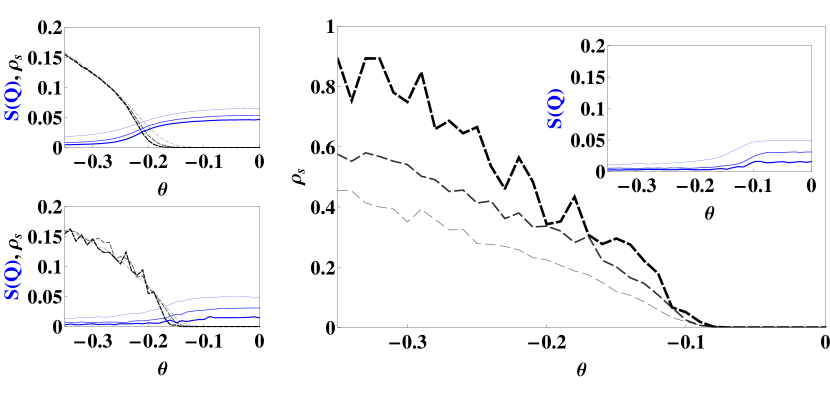
Figure 4: Cuts at $\mu/J=0$ for SR–SR (left top), LR–SR (left bottom) and LR–LR (right) for a $L=6,9$, and $12$ lattice (lines become thicker and darker with increasing system size). For all cases, the structure factor (solid blue) is finite at small $\theta$ and the superfluid fraction (dashed black) at large $\theta$. At the system sizes studied, there appears a supersolid region at intermediate $\theta$ where both structure factor and superfluid fraction are finite. In the LR–LR system there is a reversal of finite size effects. In this case the superfluid fraction for larger systems becomes higher instead of lower.

Taking “slices” out of the crystal lobes we now check where there is a supersolid region and where the system transitions directly from crystal to superfluid. Also we study the nature of these transitions to see if they are of first or second order.

The most logical region to look for supersolids is directly in between the $1/3$- and $2/3$-filling lobes, at $\mu/J=0$. Figure 4 shows the behavior of the SR–SR, the LR–SR, and the LR–LR system at this cut for several system sizes. Structure factor and superfluidity reveal, for all the systems, three different regions. In each case, the system starts at $\theta=0$ in a solid phase where the superfluid fraction is zero but the structure factor is finite. It transitions smoothly into a supersolid region where both superfluidity and structure factor are non-zero. Finally, the structure factor smoothly drops away and leaves just a non-zero superfluid fraction, making the final phase a superfluid. In each system, the size of the supersolid region is different. In the SR–SR case, the supersolid region begins to appear at $\theta\simeq-0.15$ for a $L=6$ lattice. As the size grows to $L=12$, the region has shifted to $\theta\simeq-0.19$ with the superfluid curves becoming sharper. The increased system size also reduces the value of the structure factor a little. From [29], we know that at even larger sizes (but $T=0$) the supersolid will continue to exist in this type of system. For the LR–SR system the supersolid region appears at a similar point and also shifts with system-size increase. The structure factor on the other hand has a significant decrease for larger system sizes. It is difficult to tell if at greater sizes the existence of the supersolid will persist. The final graph shows the LR–LR system. In this system, superfluidity appears even before $\mu/J$ reaches $-0.1$. In this system, the superfluid fraction is much greater than in the previous two because of the long-ranged tunneling. This means that at small system sizes the supersolid region is much more prominent relative to the crystal lobe. The structure factor diminishes with system size almost exactly as in the LR-SR case except that the transition is at a different value of $\theta$, and near $\mu/J=0$ it drops to slightly lower values. Due to this strong decrease, for any situation with long-range interactions we cannot clearly state whether the supersolid region survives at larger system sizes.

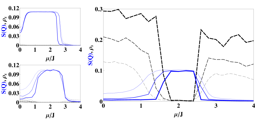
Figure 5: Cuts at $\theta=-0.15$ for SR–SR (left top), LR–SR (left bottom), LR–LR (right) for a $L=6,9$, and $12$ lattice (lines become thicker and darker with increasing system size). Solid blue: Structure Factor. Dashed black: Superfluid fraction. At this value of $\theta$, for short-range tunneling, the superfluid fraction disappears rapidly with increasing system size, while for long-range tunneling it even increases. At $\mu/J\approx 1.75$, possibly a supersolid may survive in large lattices. Again in the LR–LR system there is a reversal of finite size effects. The superfluid fraction for larger systems becomes higher instead of lower.

Next we take vertical cuts at a value of $\theta=-0.15$, since this is a reasonable place for a supersolid to exist for the LR-LR system ($\simeq 80\%$ of the tip of the lobe). We compare all the systems at this cut, and study the behavior of the superfluid fraction and the structure factor, plotted in Fig. 5. For SR–SR interactions, no supersolid region appears. On one side of the lobe there is a sharp phase transition directly from the crystal to the superfluid phase, while on the other side there is a slower change from one solid form to another ($\rho=1/3\to 2/3$). The finite-size scaling in the figure shows that as the size increases the transitions of the structure factor become even sharper, although they stay continuous due to the finite temperature. The values of the superfluid fraction decrease as the system sizes increases and essentially disappear at $L=12$. In the LR–SR system, a hint of the supersolid phase begins to appear on either side of the lobe. It is a bit more evident on the side where $\mu/J$ is small (as is to be expected from references such as [28]), but it also arises on the opposite side. This is contrary to a system of only short-ranged interactions where this supersolid region appears only on one side of the lobe and not both. At larger sizes, also in the LR–SR system the transitions become sharper and the superfluidity gets smaller. The final and most interesting cut is taken out of the LR–LR lobe. In this system, we see a smooth transition from crystal to supersolid at $\mu/J\simeq 2.4$ and at $\mu/J\simeq 1.4$ for $L=6$. For larger systems the transition at $\mu/J\simeq 2.4$ occurs at the same spot but becomes sharper, making the supersolid region disappear. At $\mu/J\simeq 1.4$ the transition shifts to a higher value of $\mu/J$, making the $2/3$-filling plateau smaller. It also becomes less smooth but the supersolid region remains longer than for the SR–SR case. In the LR–LR system, the superfluid fraction for larger systems has the opposite effect than for the previous cases, it becomes higher instead of lower.

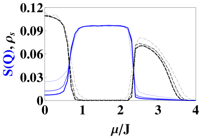
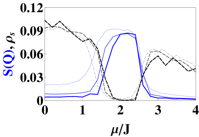
Figure 6: SR–SR (left) at $\theta=-0.28$ and LR–SR (right) at $\theta=-0.23$. Solid blue: Structure Factor. Dashed black: Superfluid fraction. Lines become thicker and darker as system size goes up. In the SR–SR system, a supersolid at small $\mu/J$ persists at large systems, while at $\mu/J\approx 2.4$ the transition from crystal to superfluid becomes a direct first-order transition. For the LR–SR system, the curves change slowly at both sides of the crystal lobe, leading to persisting supersolids.

A perhaps fairer comparison is to look at a cut through a region where we are sure the supersolid exists for all three systems. Therefore, in Fig. 6 we look at two more cuts that are now taken closer to the tips of the SR–SR and LR–SR lobes. As with the LR-LR system (last panel of Fig. 5), these lie at around $80\%$ of the tip of the lobe. In the SR–SR lobe, the cut is taken at $\theta=-0.28$. Here we see a similar behavior for the structure factor as we did in the $\theta=-0.15$ cut of the lobe, but this time the superfluid fraction plays a much more important role. On the one side, $\mu/J\simeq 2.4$, both the superfluid fraction as well as the structure factor have sharp transitions that become even sharper at larger sizes. In fact, at $T=0$ these transitions have been shown to be of first order, and the system goes directly from crystal to superfluid. Due to the finite temperature, they are continuous in our case. On the other side, where $\mu/J\simeq 0.8$, there appears a second order phase transition into a supersolid region that spans all the way to $\mu/J=0$. Finally, we take a cut at $\theta=-0.23$ of the LR–SR lobe. The behavior of this system seems to be quite different. The first thing to notice is that the transitions on either side of the lobe are of second order. The other, and more important, observation is that now it appears that this system has supersolid behavior on both sides of the lobe: in addition to the expected supersolid at smaller $\mu/J$, a region at $\mu/J$ above the crystal lobe appears where both structure factor and superfluid fraction are finite. If we recall Fig. 5, right panel, the LR–LR system showed that at $\theta=-0.15$ as $L$ increased the supersolid region disappeared from the upper side of the lobe. In the case of the LR–SR system for $\theta=-0.23$ the increase in the system size does not get rid of this supersolid phase.

3.3 Finite temperature results

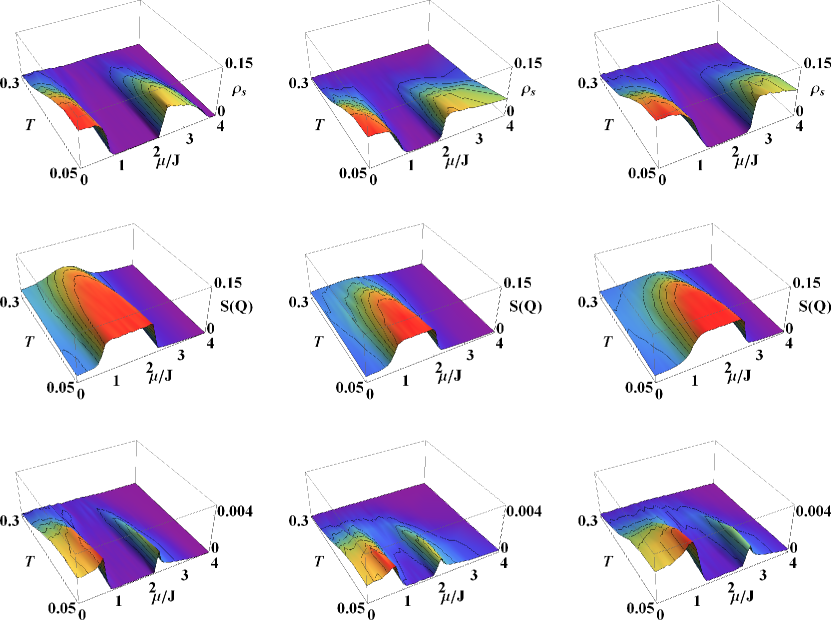
Figure 7: Each row shows a different object : the top row – the stiffness, the middle row – the structure factor while the bottom row represents a product of the first two rows. Columns corresponds to different systems: Left column is for SR–SR at $\theta=-0.28$, middle column yields LR–SR at $\theta=-0.23$, right column is for LR–LR at $\theta=-0.15$. For all three systems, the three distinct quantum phases – crystal, supersolid, and superfluid – survive over some temperature range before they melt.

As a final calculation, we take a look at the important role that the temperature plays in both the melting of the crystal as well as the supersolid region. In this section, we will use the same cuts as in the previous section ($\theta=-0.28$ for SR–SR, $\theta=-0.23$ for LR–SR and $\theta=-0.15$ for LR-LR) so that each system will posses all the possible phases: crystal, superfluid, and supersolid. Each cut is investigated for $0.05<T<0.3$ at a system size of $L=6$. First, we analyze the structure factor to study how the $\rho=2/3$ crystal melts with an increase in temperature (second row of Fig. 7). For the SR–SR interactions, even at a temperature of $0.3$ there still exists a bump in the structure factor which indicates that the crystal has not completely melted yet, while for both of the long-ranged lobes the crystal melts by $T\simeq 0.3$. Interestingly, the SR–SR crystal and the LR–LR crystal are approximately the same size at $T=0.05$, but by $T=0.3$ one has melted while the other still exists. That means that the system with short-ranged interactions holds its crystal structure better at higher temperatures than does our system with all long-ranged interactions. Looking at the LR–SR lobe, we see that its crystal at this cut starts off smaller, yet it melts at about the same temperature as the one for LR–LR interactions. It seems that the dipolar repulsion helps stabilize the crystal structure over a larger temperature range, while the long-ranged hopping destroys the crystal more quickly because of the extra kinetic energy.

Maybe more importantly, we now study the melting of the supersolid for these same cuts. Figure 7 shows the structure factor, superfluidity, and supersolidity as a function of temperature for each of the different systems. Since the supersolid is defined by having both non-zero structure factor and non-zero superfluid fraction, by combining the graphs we are able to see where these regions exist and also how they melt with increased temperature (the bottom row of Fig. 7 shows a product of structure factor and superfluid fraction, which remains finite only where the two coexist). A common feature of all the graphs are the spikes on either side of the plateaus. These are regions where a phase transition occurs but does not necessarily imply that a supersolid region exists. Most likely, these features appear due to the finite size of the system and the resulting smooth transitions of superfluid fraction and structure factor. At larger sizes, the transitions would be much sharper at these points, the regions where a finite structure factor and superfluid fraction coexist would shrink, and the spikes would diminish. From the previous section, we can assume that for the SR–SR system they would disappear completely at the upper transition from the crystal lobe while for the other two systems there would still exist a small supersolid region.

Returning to the main focus, the small-$\mu$ region, we see that in each case a supersolid region appears that extends from the left side of the plateau all the way to $\mu/J=0$. In every system, this supersolid region also exists for a finite range of temperatures. For SR–SR interactions, it gradually decreases but still extends all the way out past $T=0.3$. For the LR–SR interactions, the supersolid region again slowly melts but now disappears at $T\simeq 0.23$, just below the spot where the crystal melted. The supersolid region for the LR–LR system appears to have the largest magnitude of the three systems, but then rapidly melts at $T\simeq 0.3$.

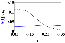
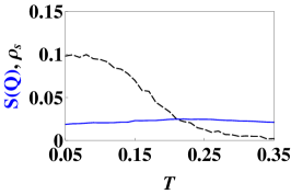
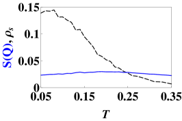
Figure 8: SR–SR at $\theta=-0.28$, LR–SR at $\theta=-0.23$ and LR–LR at $\theta=-0.15$ (left to right). All cuts are taken at $\mu/J=0$. The structure factor (solid blue) attains similar values for all three systems. The superfluid fraction (dashed black) is largest in the LR–LR system and melts fastest in the LR–SR one.

In order to compare these transitions more quantitatively, we take a cut along $\mu/J=0$ for each system, shown in Fig. 8. All three systems show a relatively similar and steady value for the structure factor. Hence, the values of the superfluid fraction are going to determine the existence of the supersolid regions. The first plot shows the SR–SR system at the $\theta=-0.28$ cut, and we can see that the superfluid fraction stays non-zero all the way out to $T=0.35$. The LR–SR system has a very similar behavior at the $\theta=-0.23$ cut, but in this case the supersolid is nearly completely melted by $T=0.35$. The final plot is the LR–LR system at $\theta=-0.15$, which behaves slightly differently. The most important difference is that the starting value of the superfluid fraction is higher than in the first two plots. This should therefore make the supersolid region more pronounced. But even though the superfluid fraction has the highest value for this system, it decays more quickly and reaches values similar to the SR–SR system at $T\approx 0.35$.

4 Conclusion

In this paper, we have presented a quantum Monte Carlo study of dipolar spin models that describe various systems of ultracold atoms, molecules, and ions. We have presented predictions concerning the phase diagram of the considered systems at zero and finite temperatures, and described the appearance and some properties of the superfluid, supersolid, and crystalline phases. While the results are not surprising and resemble earlier obtained results for similar systems in 1D and 2D, the main advantage of our study is that it is directly relevant to the current experiments:

• The results for the XXZ model with short-range tunneling apply for ultracold gases of polar bosonic molecules in the limit of hard-core bosons. Note that the earlier works [15, 16] have concentrated on the appearance of the supersolid phase and devil’s staircase of crystalline phases in the square lattice [15], and supersolid and emulsion phases in the triangular lattice [16]. Here we focus on the hard-core-spin limit, and compare it and stress differences with other models, such as the ones with long-range tunneling, i.e., long-range XX interactions.

• The results for the XXZ models with long-range tunneling apply for systems of trapped ions in triangular lattices of microtraps. These results are novel, since so far such models have been only studied using various techniques in 1D, and using the mean-field approach in 2D. While the first experimental demonstrations of such models were restricted to a few ions (see for instance [3]), many experimental groups are working on an extension of such ionic quantum simulators to systems of many ions in microtraps [37]. In fact, very recently the NIST group has engineered 2D Ising interactions in a trapped-ion quantum simulator with hundreds of spins [38]. Although in this experiment the quantum regime has not yet been achieved, it clearly opens the way toward quantum simulators of spin models with long-range interactions. We expect that in the near future the result of our present theoretical study will become directly relevant for experiments.

References

References

- [1] R. P. Feynman, Int. J. Theor. Phys. 21, 467 (1982).
- [2] P. Hauke, F. M. Cucchietti, L. Tagliacozzo, I. Deutsch and M. Lewenstein, Rep. Prog. Phys. 75, 082401 (2012).
- [3] A. Friedenauer, H. Schmitz, J. T. Glückert, D. Porras and T. Schätz, Nature Physics 4, 757 - 761 (2008).
- [4] K. Kim, M.S. Chang, S. Korenblit, R. Islam, E. E. Edwards, J. K. Freericks, G.D. Lin, L.M. Duan and C. Monroe, Nature 465, 590 (2010).
- [5] D. Porras and J. I. Cirac, Phys. Rev. Lett. 92, 207901 (2004).
- [6] F. Mintert and C. Wunderlich, Phys. Rev. Lett. 87, 257904 (2001).
- [7] D. Porras and J. I. Cirac, Phys. Rev. Lett. 96, 250501 (2006).
- [8] P. Hauke, F. M. Cucchietti, A. Müller-Hermes, M. Bañuls, J. I. Cirac and M. Lewenstein, New J. Phys. 12, 113037 (2010).
- [9] D. Peter, S. Müller, S. Wessel and H. P. Büchler, Phys. Rev. Lett. 109, 025303 (2012).
- [10] R. Barnett, D. Petrov, M. Lukin and E. Demler, Phys. Rev. Lett. 96, 190401 (2006).
- [11] A. V. Gorshkov, S. R. Manmana, G. Chen, J. Ye, E. Demler, M. D. Lukin and A. M. Rey, Phys. Rev. Lett. 107, 115301 (2011).
- [12] E. G. Dalla Torre, E. Berg and E. Altman, Phys. Rev. Lett. 97, 260401 (2006).
- [13] G. G. Batrouni, F. Hébert and R. T. Scalettar, Phys. Rev. Lett. 97, 087209 (2006).
- [14] P. Sengupta, L. P. Pryadko, F. Alet, M. Troyer and G. Schmid, Phys. Rev. Lett. 94, 207202 (2005).
- [15] B. Capogrosso-Sansone, C. Trefzger, M. Lewenstein, P. Zoller and G. Pupillo, Phys. Rev. Lett. 104, 125301 (2010).
- [16] L. Pollet, J. D. Picon, H.P. Büchler, and M. Troyer, Phys.Rev.Lett. 104, 125302 (2010).
- [17] C. Menotti, C. Trefzger and M. Lewenstein, Phys. Rev. Lett. 98, 235301 (2007).
- [18] C. Trefzger, C. Menotti and M. Lewenstein, Phys. Rev. A 78, 043604 (2008).
- [19] T. Lahaye, C. Menotti, L. Santos, M. Lewenstein and T. Pfau, Rep. Prog. Phys. 72, 126401 (2009).
- [20] T. Ohgoe, T. Suzuki and N. Kawashima, arXiv:1110.2109v2 (2012).
- [21] P. Bak R. and Bruinsma, Phys. Rev. Lett. 49, 249 (1982).
- [22] X. L. Deng, D. Porras and J. I. Cirac, Phys. Rev. A 72, 063407 (2005).
- [23] J. Freericks and H. Monien, Phys. Rev. B 53, 2691 (1996).
- [24] M. Maik, P. Buonsante, A. Vezzani and J. Zakrzewski, Phys. Rev. A 84, 053615 (2011).
- [25] R. Citro, E. Orignac, S. De Palo and M. L. Chiofalo, Phys. Rev. A 75, 051602(R) (2007).
- [26] R. Citro, S. De Palo, E. Orignac, P. Pedri and M. L. Chiofalo, New J. Phys. 10, 045011 (2008).
- [27] M. Dalmonte, G. Pupillo and P. Zoller, Phys. Rev. Lett. 105, 140401 (2010).
- [28] S. Wessel and M. Troyer, Phys. Rev. Lett. 95, 127205 (2005).
- [29] D. Heidarian and K. Damle, Phys. Rev. Lett. 95, 127206 (2005).
- [30] R. G. Melko, A. Paramekanti, A. A. Burkov, A. Vishwanath, D. N. Sheng and L. Balents, Phys. Rev. Lett. 95, 127207 (2005).
- [31] N. D. Mermin and H. Wagner, Phys. Rev. Lett. 17, 1133 (1966).
- [32] C. Lhuillier, arXiv:0502464v1 (2005).
- [33] F. J. Burnell, M. M. Parish, N. R. Cooper and S. L. Sondhi, Phys. Rev. B 80, 174519 (2009).
- [34] B. Bauer, L. D. Carr, H. G. Evertz, A. Feiguin, J. Freire, S. Fuchs, L. Gamper, J. Gukelberger, E. Gull, S. Guertler, A. Hehn, R. Igarashi, S. V. Isakov, D. Koop, P. N. Ma, P. Mates, H. Matsuo, O. Parcollet, G. Pawłowski, J. D. Picon, L. Pollet, E. Santos, V. W. Scarola, U. Schollwöck, C. Silva, B. Surer, S. Todo, S. Trebst, M. Troyer, M. L. Wall, P. Werner and S. Wessel, J. Stat. Mech. P05001 (2011).
- [35] N. V. Prokof’ev, B. V. Svistunov and I. S.Tupitsyn, Phys. Lett. A 238, 253 (1998).
- [36] H. Ozawa and I. Ichinose, arXiv:1204.6114v1 (2012).
- [37] D. Wineland, C. Monroe, T. Schätz, R. Blatt, private communication.
- [38] J.W. Britton, B.C. Sawyer, A.C. Keith, C.-C.J. Wang, J.K. Freericks, H. Uys, M.J. Biercuk and J.J. Bollinger, Nature 484, 489 (2012).