Abstract

The time evolution of a Gamma-ray burst (GRB) is associated with the evolution of a supernova remnant (SNR). The time evolution of the flux of a GRB is modeled introducing a law for the density of the medium in the advancing layer. The adopted radiative model for the GRB in the various e.m. frequencies is synchrotron emission. The X-ray ring which appears a few hours after a GRB is simulated.

Adv. Studies Theor. Phys, Vol. x, 200x, no. xx, xxx - xxx

Direct conversion of the flux of kinetic energy

into radiation in gamma-ray burst

L. Zaninetti

Dipartimento di Fisica Generale,

Università degli Studi di Torino,

via P. Giuria 1, 10125 Torino, Italy

PACS: 98.70.Rz , 07.85.-m
Keywords: Gamma-ray bursts, Gamma-ray sources

1 Introduction

Gamma-ray bursts (GRBs) started to be observed from an astronomical point of view by [1]. Recently some excellent reviews have been written, see [2, 3, 4, 5]. The recent trend of research connects GRBs with supernovae (SN) explosions and their consequent remnants (SNRs). The afterglow is observed in X, optical, and infrared, see [6]. The established connection between GRBs and SNRs allows of restricting the astrophysical environment to the advancing shock. In the last 60 years the theoretical studies of the advancing shock of SNR have been focused on the relationship with the instantaneous radius of expansion, $R$, which is of type $\propto~{}t^{m}$, where $t$ is time and $m$ is a parameter that depends on the chosen model. The most popular model is the Sedov–Taylor expansion which predicts $R\propto t^{0.4}$, see [7, 8, 9, 10], and the thin layer approximation in the presence of a constant density medium, which predicts $R\propto t^{0.25}$, see [11]. A simple version of the Sedov–Taylor solution, which also considers the transition from the relativistic to the non-relativistic regime, appeared in [12, 2]. The radiative transfer during the afterglow phase has been analysed by [13], where a comprehensive analysis, including images of the expected light curves, is carried out. The actual situation of the theoretical and observational research on SNRs leaves a series of questions unanswered or only partially answered:

• Can we deduce a theoretical expression for the counts/s versus time in a GRB assuming a direct proportionality between the flux of kinetic energy of the advancing shell and the intensity of emission?

• Can we simulate the X-ray ring of GRB 032103, which was observed six hours after the burst?

• Can we deduce a theoretical expression for the frequency at which the GRB becomes visible as a function of the time?

In order to answer these questions, Section 2 reports the data on GRBs. Section 3 reviews the free expansion, the Sedov–Taylor solution and the power law model. Section 4 reviews the existing situation about the radiative transport equation and a simple geometrical model which leads to the ring emission. Section 5 contains some scaling arguments that lead to the observed count/s versus time relationship.

2 The Observations of GRBs

GRBs are characterized by a rapid rise (called the trigger) in the rate of detected photons per second at a given energy, for example 20 kev. A typical example observed by the Burst and Transient Source Experiment (BATSE), see [14], on board the Compton Gamma Ray Observatory (CGRO) is reported in Fig. 1.

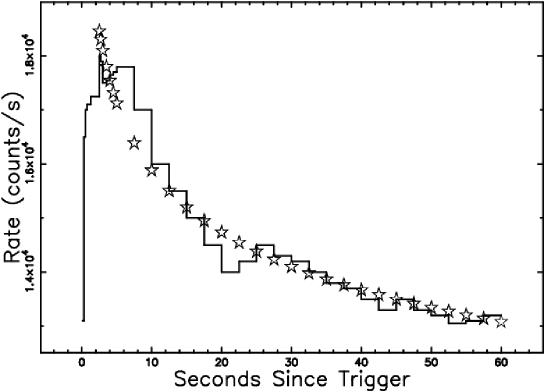
Figure 1: Light curve of BATSE trigger 8121 in the energy channels 1–4 ( $>$ 20 kev) (full line) and power law fit (empty stars). The real data have been extracted by the author from the BATSE database available at the web site http://www.batse.msfc.nasa.gov/batse/grb/lightcurve/ . In this case $\delta=-0.1086$ and $C=20382.27$ when  $t~{}\geq$  1.25  s.

¿From the previous figure it is important to point out that the time necessary to reach the maximum is 1.25 s. In the following we will consider this time small compared to the time in which the counts/s decreases.

A numerical analysis of the observed rate versus time relationship can be done by assuming a power law dependence for the rate of counts of the type

$$rate(t)=Ct^{\delta}~{}counts~{}s^{-1}\quad,$$ (1)

where the two parameters $C$ and $\delta$ are found from a numerical analysis of the data.

An interesting analysis of the time evolution of 12 GRBs as observed by the Swift Gamma-Ray Burst Mission (Swift), see [15], is reported in [16]. We selected one GRB from the previous list, namely, GRB050814 XRT 1.5–10 kev which is visible in Fig. 3 (top-right) of [16]. For the previous GRB as well the fit with relationship (1) is reported in Fig. 2.

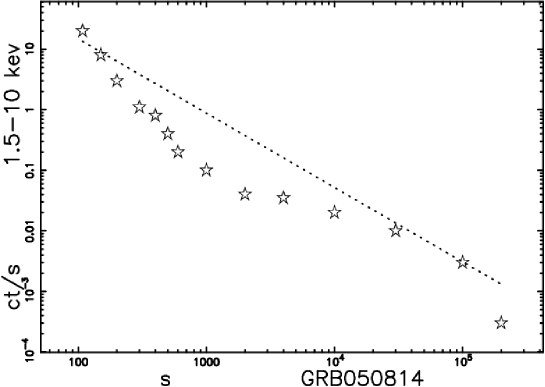
Figure 2: Light curve of GRB050814 XRT 1.5–10 kev (empty stars) and power law fit (dotted line). The real data have been extracted by the author from Fig. 3 (top-right) of Willingale et al. 2010. In this case $\delta=-1.22$ and $C=4214$.

The count spectrum in energy of GRB 080916C, see [17], is reported in Fig. 3 and

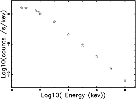
Figure 3: Count spectrum in energy as measured by the three instruments on board the Fermi Gamma-ray Space Telescope, which are Nal, BGO, and LAT. The data are extracted by the author from Fig. 2A in [17].

can be approximated by the following formula

$$E(kev)\approx 1563E(kev)^{-1.7}\quad when\quad 10~{}kev~{}\leq E\leq 10^{7}kev.$$ (2)

Another interesting property of the GRBs is that the frequency of observation at which they start to be visible decreases with time. An example of such behaviour for GRB 050904 in the BAT, XRT, J, and I bands can be found in Table 1 of [18]. The numerical analysis of the data in Fig. 4 gives

$$\nu=1.0310^{25}t(s)^{-2.27}\,Hz$$ (3)

where $t$ has been chosen as the value of time at which the flux at the chosen frequency is maximal.

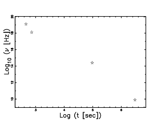
Figure 4: Bands from the radio through the IR/optical to X-ray and BAT at which the expansion becomes optically thin. The energy bands are expressed in logarithms of the frequency in Hz along the $y$-axis. The $x$-axis reports the logarithm of the time in seconds. The data are extracted by the author from Table 1 in [18].

Also interesting is the case of GRB 032103, which was observed in the X-ray (energy range 0.7–2.5 keV) by XMM-Newton’s MOS cameras six hours after the GRB, see [19]. In this case the combined MOS images show two concentric rings which expand outwards. The numerical analysis gives $\theta\propto(t-t_{0})^{1/2}$ where $\theta$ is the angular separation between the the two maxima in the radial profiles of counts, $t$ is the time, and $t_{0}$ the initial time. In the following we will associate the GRBs with the explosions of supernovae which are classified as SNR, see Section 4 in [4].

3 Some existing solutions

This section reviews the expansion at constant velocity, the Sedov–Taylor, and the power law models.

3.1 The constant expansion velocity model

The SNR expands at a constant velocity until the surrounding mass is of the order of the solar mass. This time, $t_{M}$, is

$$t_{M}=186.45\,{\frac{\sqrt[3]{{\it M_{\odot}}}}{\sqrt[3]{{\it n_{0}}}{\it v_{10000}}}}\quad\mathrm{yr}\quad,$$ (4)

where $M_{\odot}$ is the number of solar masses in the volume occupied by the SNR, $n_{0}$, the number density expressed in particles $\mathrm{cm}^{-3}$, and $v_{10000}$ the initial velocity expressed in units of 10 000 km/s, see [20].

3.2 The Sedov–Taylor solution

3 The Sedov–Taylor solution is

$$R(t)=\left({\frac{25}{4}}\,{\frac{{\it E}\,{t}^{2}}{\pi\,\rho}}\right)^{1/5}\quad,$$ (5)

where $E$ is the energy injected into the process and $t$ is time, see [8, 9, 10, 20]. Our astrophysical units are: time, ($t_{1}$), which is expressed in years; $E_{51}$, the energy in $10^{51}$ erg; $n_{0}$, the number density expressed in particles $\mathrm{cm}^{-3}$  (density $\rho=n_{0}$m, where m = 1.4$m_{\mathrm{H}}$). In these units, Equation (5) becomes

$$R(t)\approx 0.313\,\sqrt[5]{{\frac{{\it E_{51}}\,{{\it t_{1}}}^{2}}{{\it n_{0}}}}}~{}{pc}\quad.$$ (6)

The Sedov–Taylor solution scales as $t^{0.4}$. We are now ready to couple the Sedov–Taylor phase with the free expansion phase

$$R(t)=\left\{\begin{array}[]{ll}0.0157\,{\it t}\,\mathrm{pc}&\mbox{if $t\leq 2.5$ yr }\\ 0.0273\,\sqrt[5]{{{\it t}}^{2}}\,\mathrm{pc}&\mbox{if $t>2.5$\ yr.}\end{array}\right.$$ (7)

This two-phase solution is obtained with the following parameters $M_{\odot}=1$, $n_{0}=1.127\,10^{5}$, $E_{51}=0.567$ and Fig. 5 reports its temporal behaviour as well as the data.

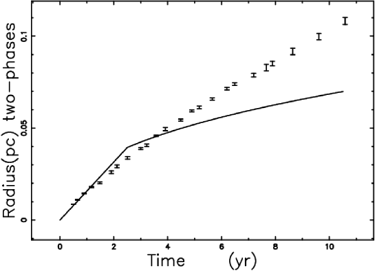
Figure 5: Theoretical radius as given by the two-phase solution (full line), and astronomical data of SN 1993J with vertical error bars.

¿From the previous figure, it is clear that the free expansion plus the Sedov–Taylor phase is not a satisfactory model.

3.3 The power law model

We shall discuss a power law dependence of the type

$$R(t)=Ct^{\alpha}\quad,$$ (8)

where the two parameters $C$ and $\alpha$ can be found from the observations. Ten years of observations of SN 1993J , see [21], allow of fixing these two parameters: $\alpha=0.828\pm 0.0048$ and $C=0.0155\pm 0.00011$, and Figure 6 displays the data as well as the fit.

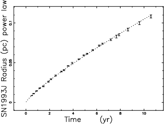
Figure 6: Theoretical radius as given by the power law model (full line), and astronomical data of SN 1993J with vertical error bars.

This observed relationship allows of expressing, from an astrophysical point of view, the radius as

$$R(t)=0.0155\,{t}^{0.828}\quad pc\quad,$$ (9)

where the time $t$ is expressed in years. The velocity in this model is

$$V(t)=C\,\alpha t^{(\alpha-1)}$$ (10)

and the astrophysical version

$$V(t)=12587.67\,{t}^{-0.171}\frac{\mathrm{km}}{\mathrm{s}}\quad.$$ (11)

Figure 7 reports the observed instantaneous velocity as deduced from the finite difference method and the best fit according to (11).

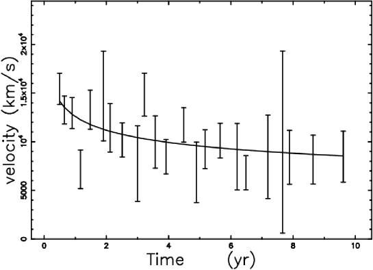
Figure 7: Theoretical velocity as given by Eq. (11) (full line) and instantaneous velocity of SN 1993J with uncertainty.

4 Radiative processes

This section reviews the existing knowledge about the transfer equation and a simple model which produces an X-ring.

4.1 The transfer equation

The transfer equation in the presence of emission only, see for example [22] or [23], is

$$\frac{dI_{\nu}}{ds}=-k_{\nu}\rho I_{\nu}+j_{\nu}\rho\quad,$$ (12)

where $I_{\nu}$ is the specific intensity, $s$ is the line of sight, $j_{\nu}$ is the emission coefficient, $k_{\nu}$ is a mass absorption coefficient, $\rho$ is the density of mass at position $s$, and the index $\nu$ denotes the frequency of emission of interest. The intensity of radiation, i.e., the photon flux, is here identified with the counts at a given energy. The solution to Equation (12) is

$$I_{\nu}(\tau_{\nu})=\frac{j_{\nu}}{k_{\nu}}(1-e^{-\tau_{\nu}(s)})\quad,$$ (13)

where $\tau_{\nu}$ is the optical depth at frequency $\nu$:

$$d\tau_{\nu}=k_{\nu}\rho ds\quad.$$ (14)

The framework of synchrotron emission, as described in sec. 4 of [24], is often used in order to explain a GRB, see for example [25, 26, 27, 28]. The volume emissivity (power per unit frequency interval per unit volume per unit solid angle) of the ultrarelativistic radiation from a group of electrons, according to [29], is

$$\epsilon(\nu)=\int P(\nu)N(E)dE\quad,$$ (15)

where $P(\nu)$ is the total power radiated per unit frequency interval by one electron and $N(E)dE$ is the number of electrons per unit volume, per unit solid angle along the line of sight, which are moving in the direction of the observer and whose energies lie in the range $E$ to $E+dE$. In the case of a power law spectrum,

$$N(E)dE=KE^{-\gamma}dE\quad,$$ (16)

where $K$ is a constant. The value of the constant $K$ can be found by assuming that the probability density function (PDF, in the following) for relativistic energy is of Pareto type as defined in [30]:

$$f(x;a,c)={ca^{c}}{x^{-(c+1)}}\quad,$$ (17)

with $c~{}>0$. In our case, $c=\gamma-1$ and $a=E_{min}$, where $E_{min}$ is the minimum energy. ¿From the previous formula, we can extract

$$K=N_{0}(\gamma-1)E_{min}^{\gamma-1}\quad,$$ (18)

where $N_{0}$ is the total number of relativistic electrons per unit volume, here assumed to be approximately equal to the matter number density. The previous formula can also be expressed as

$$K=\frac{\rho}{1.4\,m_{\mathrm{H}}}(\gamma-1)E_{min}^{\gamma-1}\quad,$$ (19)

where $m_{H}$ is the mass of hydrogen. The emissivity of the ultrarelativistic synchrotron radiation from a homogeneous and isotropic distribution of electrons whose $N(E)$ is given by Equation (16) is, according to [29],

$$j_{\nu}\rho=$$ (20)

$$\approx 0.933\times 10^{-23}\alpha_{L}(\gamma)KH_{\perp}^{(\gamma+1)/2}\bigl{(}\frac{6.26\times 10^{18}}{\nu}\bigr{)}^{(\gamma-1)/2}$$

$$\mathrm{ergsec}^{-1}\mathrm{cm}^{-3}\mathrm{Hz}^{-1}\mathrm{rad}^{-2}\quad,$$

where $\nu$ is the frequency and $\alpha_{L}(\gamma)$ is a slowly varying function of $\gamma$ which is of the order of unity and is given by

$$\alpha_{L}(\gamma)=2^{(\gamma-3)/2}\frac{\gamma+7/3}{\gamma+1}\Gamma\bigl{(}\frac{3\gamma-1}{12}\bigr{)}\Gamma\bigl{(}\frac{3\gamma+7}{12}\bigr{)}\quad,$$ (21)

for $\gamma\geq\frac{1}{2}$.

We now continue to analyse the case of an optically thin layer in which $\tau_{\nu}$ is very small (or $k_{\nu}$ is very small) and where the density $\rho$ is replaced by the concentration $C(s)$ of relativistic electrons:

$$j_{\nu}\rho=K_{e}C(s)\quad,$$ (22)

where $K_{e}$ is a constant function of the energy power law index, magnetic field, and frequency of e.m. emission. The intensity is now

$$I_{\nu}(s)=K_{e}\int_{s_{0}}^{s}C(s\prime)ds\prime\quad\mbox{optically thin layer}.$$ (23)

The increase in brightness is proportional to the concentration integrated along the line of sight.

4.2 The X-ring

We assume that the number density of ultrarelativistic electrons $C$ is constant and in particular rises from 0 at $r=a$ to a maximum value $C_{m}$, remains constant up to $r=b$, and then falls again to 0. This geometrical description is reported in Fig. 8.

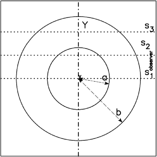
Figure 8: The two circles (sections of spheres) which include the region with constant density are represented through a full line. The observer is situated along the $x$ direction, and three lines of sight are indicated.

The length of sight, when the observer is situated at the infinity of the $x$-axis, is the locus parallel to the $x$-axis which crosses the position $y$ in a Cartesian $x--y$ plane and terminates at the external circle of radius $b$. The locus length is

$$l_{0a}=2\times(\sqrt{b^{2}-y^{2}}-\sqrt{a^{2}-y^{2}})\quad;0\leq y<a$$

$$l_{ab}=2\times(\sqrt{b^{2}-y^{2}})\quad;a\leq y<b\quad.$$ (24)

When the number density of ultrarelativistic electrons $C_{m}$ is constant between two spheres of radius $a$ and $b$ the intensity of radiation is

$$I_{0a}=C_{m}\times 2\times(\sqrt{b^{2}-y^{2}}-\sqrt{a^{2}-y^{2}})\quad;0\leq y<a$$

$$I_{ab}=C_{m}\times 2\times(\sqrt{b^{2}-y^{2}})\quad;a\leq y<b\quad.$$ (25)

The ratio between the theoretical intensity at the maximum $(y=a)$ and at the minimum ($y=0$) is given by

$$\frac{I(y=a)}{I(y=0)}=\frac{\sqrt{b^{2}-a^{2}}}{b-a}\quad.$$ (26)

The parameter $b$ is identified with the external radius which denotes the transition from the perturbed medium. The parameter $a$ can be found from the following formula:

$$a=\frac{b\left((\frac{I(y=a)}{I(y=0)})_{obs}^{2}-1\right)}{\left((\frac{I(y=a)}{I(y=0)})_{obs}^{2}+1\right)}\quad,$$ (27)

where $(\frac{I(y=a)}{I(y=0)})_{obs}$ is the observed ratio between the maximum intensity at the rim and the intensity at the centre. A cut in the theoretical intensity of GRB 031203 XMM-Newton is reported in Fig. 9 and a theoretical image in Fig. 10.

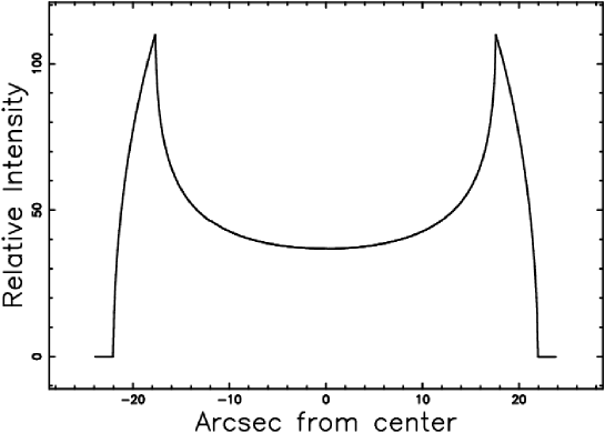
Figure 9: Cut of the mathematical intensity ${\it I}$ of the ring model, Equation (25), crossing the centre (full line) of GRB 031203 XMM-Newton observation. The $x$- and $y$-axes are in arcsec, $a=17.6$ arcsec, $b=22$ arcsec and $\frac{I(y=a)}{I(y=0)}=3$ as in Fig. 2 panel 6 of [19].

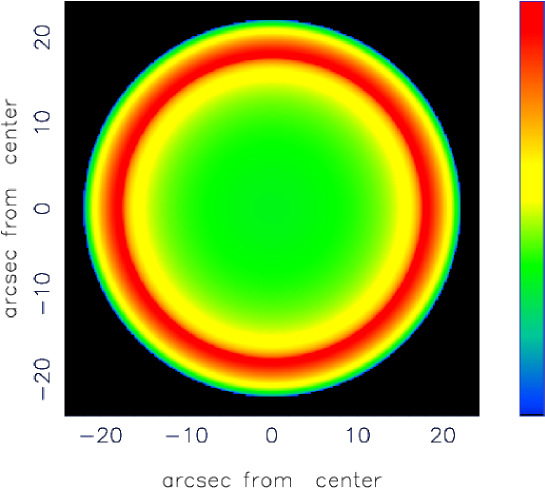
Figure 10: Contour map of ${\it I}$ adjusted to simulate GRB 031203 XMM-Newton observation. The $x$ and $y$ axes are in arcsec, other parameters as in Fig. 9.

A comparison should be made with Fig. 7 in [13].

5 Flux density versus time

The source of synchrotron luminosity is assumed here to be the flux of kinetic energy, $L_{m}$:

$$L_{m}=\frac{1}{2}\bar{\rho_{L}}\pi R^{2}V^{3}\quad,$$ (28)

where $R$ is the instantaneous radius of the SNR, and $\bar{\rho_{L}}$ is the averaged density in the advancing layer. The averaged density in the advancing layer can be parametrized as

$$\bar{\rho_{L}}=\frac{(\rho\frac{4}{3}\pi R^{3})^{1/p}}{4\pi R^{2}\Delta R}\quad,$$ (29)

where $\Delta R$ is the thickness of the advancing radius in which the mass resides. In order to quantify the thickness we assume that

$$\Delta R=\frac{R(t)^{\eta_{I}}}{n}\quad,$$ (30)

with $\eta_{I}$ derived from the fit with the observations and $n$ a sufficiently large number such that

$$\frac{R(t_{max})^{\eta_{I}}}{n}\ll R(t_{max})\quad,$$ (31)

where $t_{max}$ is the maximum time considered.

Therefore, the mechanical luminosity transforms to

$$L_{m}\propto\bar{\rho_{L}}R^{3}V^{3}\quad.$$ (32)

The temporal and velocity evolutions can be given by the power law dependencies of Equations (8) and (10) and therefore

$$L_{m}\propto t^{-\frac{6+{\eta_{I}}p}{3+p}}\quad.$$ (33)

The synchrotron luminosity $L_{\lambda}$ and the observed flux $S_{\lambda}$ at a given wavelength $\lambda$ are assumed to be proportional to the mechanical luminosity, and therefore

$$S_{\lambda}=S_{0}(\frac{t}{t_{S0}})^{-\frac{6+{\eta_{I}}p}{3+p}}\quad,$$ (34)

where $S_{0}$ is the observed flux at $t=t_{S0}$. As an example from the astronomical data of Fig. 2, we deduce that ${\eta_{I}}=1.095$. The progressive transparency of the GRB to the low frequencies with time can be explained by the dispersion relation of an e.m. wave in a cold plasma, which is

$$\omega^{2}=\omega_{pe}^{2}+k^{2}c^{2}\quad,$$ (35)

where $\omega$ is the frequency of the e.m. wave, $\omega_{pe}$ is the plasma frequency of the electrons, $k$ is the wave-vector of the e.m. wave, and $c$ is the velocity of light, see [31]. The plasma frequency of the electrons is

$$\omega_{pe}=(4\pi n_{e}e^{2}/m_{e})^{1/2}\quad,$$ (36)

or

$$f_{pe}=\omega_{pe}/2\pi=8.98\times 10^{3}{n_{e}}^{1/2}\,\rm Hz\quad,$$ (37)

where $f_{pe}$ is the electron plasma frequency expressed in Hz. A visual inspection of the dispersion relation (35) allows us to say that in an astrophysical environment in which the number density of the electrons is decreasing with time, the frequency at which the medium becomes transparent will also progressively decrease. The time dependence of the frequency at which the medium is transparent, according to (29), is

$$\nu\propto t^{-1/2\,{\frac{-3+2\,p+{\eta_{II}}\,p}{3+p}}}\quad,$$ (38)

where $\eta_{II}$ is the same parameter as in (30) and the index $II$ means a second way to deduce the free parameter. A comparison of the previous formula with the observational formula (3) gives $\eta_{II}=3.42$.

6 Conclusions

The first two parts of the law of motion for a SNR are thought to be a free expansion in which $R\propto t$ and an energy conserving phase, the so called Sedov–Taylor phase, in which $R\propto t^{2/5}$. A careful analysis of SN 1993J in the first ten years suggests instead that $R\propto t^{0.82}$.

The scaling laws of the flux of GRBs with time can be consequently deduced assuming that the intensity of emission is proportional to the flux of the kinetic energy of the advancing shell, see Equation (34). This result is reached assuming that the thickness of the advancing layer increases $\propto~{}R^{\eta}$. The comparison between the observed flux and the time of GRB050814 XRT 1.5–10 kev gives ${\eta_{I}}=1.095$ and the comparison between the e.m. frequency of transparency and time gives $\eta_{II}=3.42$. The X-ray ring connected with GRB 031203 XMM-Newton is simulated introducing two hypotheses: (i) the emission of radiation is localized in a thin layer of the advancing expansion, (ii) the emitting medium is supposed to be optically thin.

References

- [1] R. W. Klebesadel, I. B. Strong, R. A. Olson, Observations of Gamma-Ray Bursts of Cosmic Origin, ApJ 182 (1973), L85+.
- [2] J. van Paradijs, C. Kouveliotou, R. A. M. J. Wijers, Gamma-Ray Burst Afterglows, ARA&A 38 (2000), 379–425.
- [3] P. Mészáros, Theories of Gamma-Ray Bursts, ARA&A 40 (2002), 137–169.
- [4] T. Piran, The physics of gamma-ray bursts, Rev. Mod. Phys. 76 (2004), 1143–1210.
- [5] N. Gehrels, E. Ramirez-Ruiz, D. B. Fox, Gamma-Ray Bursts in the Swift Era, ARA&A 47 (2009), 567–617.
- [6] L. P. Xin, W. K. Zheng, J. Wang, J. S. Deng, Y. Urata, Y. L. Qiu, K. Y. Huang, J. Y. Hu, J. Y. Wei, GRB 070518: a gamma-ray burst with optically dim luminosity, MNRAS 401 (2010), 2005–2011.
- [7] L. I. Sedov, Propagation of strong shock waves, Prikl. Mat. i Mekh 10 (1946), 241– 250.
- [8] G. Taylor, The Formation of a Blast Wave by a Very Intense Explosion. I. Theoretical Discussion, Royal Society of London Proceedings Series A 201 (1950), 159–174.
- [9] G. Taylor, The Formation of a Blast Wave by a Very Intense Explosion. II. The Atomic Explosion of 1945, Royal Society of London Proceedings Series A 201 (1950), 175–186.
- [10] L. I. Sedov, Similarity and Dimensional Methods in Mechanics, Academic Press, New York, 1959.
- [11] Dyson, J. E. and Williams, D. A., The physics of the interstellar medium, Institute of Physics Publishing, Bristol, 1997.
- [12] Y. F. Huang, Z. G. Dai, T. Lu, A generic dynamical model of gamma-ray burst remnants, MNRAS 309 (1999), 513–516.
- [13] J. Granot, T. Piran, R. Sari, Images and Spectra from the Interior of a Relativistic Fireball, ApJ 513 (1999), 679–689.
- [14] S. D. Barthelmy, L. M. Barbier, J. R. Cummings, E. E. Fenimore, The Burst Alert Telescope (BAT) on the SWIFT Midex Mission, Space Science Reviews 120 (2005), 143–164.
- [15] N. Gehrels, G. Chincarini, P. Giommi, K. O. Mason, J. A. Nousek, A. A. Wells, The Swift Gamma-Ray Burst Mission, ApJ 611 (2004), 1005–1020.
- [16] R. Willingale, F. Genet, J. Granot, P. T. O’Brien, The spectral-temporal properties of the prompt pulses and rapid decay phase of gamma-ray bursts, MNRAS 403 (2010), 1296–1316.
- [17] A. A. Abdo, M. Ackermann, M. Arimoto, K. Asano, W. B. Atwood, Fermi Observations of High-Energy Gamma-Ray Emission from GRB 080916C, Science 323 (2009), 1688–.
- [18] L. Gou, D. B. Fox, P. Mészáros, Modeling GRB 050904: Autopsy of a Massive Stellar Explosion at z=6.29, ApJ 668 (2007), 1083–1102.
- [19] D. Watson, J. Hjorth, A. Levan, P. Jakobsson, P. T. O’Brien, J. P. Osborne, K. Pedersen, J. N. Reeves, J. A. Tedds, S. A. Vaughan, M. J. Ward, R. Willingale, A Very Low Luminosity X-Ray Flash: XMM-Newton Observations of GRB 031203, ApJ 605 (2004), L101–L104.
- [20] R. A. McCray, Coronal interstellar gas and supernova remnants, in: A. Dalgarno & D. Layzer (Ed.), Spectroscopy of Astrophysical Plasmas, 1987, 255–278.
- [21] J. M. Marcaide, I. Martí-Vidal, A. Alberdi, M. A. Pérez-Torres, A decade of SN 1993J: discovery of radio wavelength effects in the expansion rate, A&A 505 (2009), 927–945.
- [22] G. Rybicki, A. Lightman, Radiative Processes in Astrophysics, Wiley-Interscience, New-York, 1991.
- [23] Hjellming, R. M., Radio stars IN Galactic and Extragalactic Radio Astronomy , Springer-Verlag, New York, 1988.
- [24] R. Schlickeiser, Cosmic ray astrophysics, Springer, Berlin, 2002.
- [25] A. Pe’er, B. Zhang, Synchrotron Emission in Small-Scale Magnetic Fields as a Possible Explanation for Prompt Emission Spectra of Gamma-Ray Bursts, ApJ 653 (2006), 454–461.
- [26] C. D. Dermer, Nonthermal Synchrotron Radiation from Gamma-Ray Burst External Shocks and the X-Ray Flares Observed with Swift, ApJ 684 (2008), 430–448.
- [27] M. Ackermann, K. Asano, W. B. Atwood, M. Axelsson, L. Baldini, J. Ballet, a. et, Fermi Observations of GRB 090510: A Short-Hard Gamma-ray Burst with an Additional, Hard Power-law Component from 10 keV TO GeV Energies, ApJ 716 (2010), 1178–1190.
- [28] T. Piran, E. Nakar, On the External Shock Synchrotron Model for Gamma-ray Bursts’ GeV Emission, ApJ 718 (2010), L63–L67.
- [29] K. R. Lang, Astrophysical formulae. (Third Edition), Springer, New York, 1999.
- [30] M. Evans, N. Hastings, B. Peacock, Statistical Distributions - third edition, John Wiley & Sons Inc, New York, 2000.
- [31] G. Schmidt, Physics of high temperature plasmas , Academic Press, Inc., New York, 1979.