Optimally robust shortcuts to population inversion in two-level quantum systems

Abstract

We examine the stability versus different types of perturbations of recently proposed shortcuts-to-adiabaticity to speed up the population inversion of a two-level quantum system. We find optimally robust processes using invariant based engineering of the Hamiltonian. Amplitude noise and systematic errors require different optimal protocols.

1 Introduction

Manipulating the state of a quantum system with time-dependent interacting fields is a fundamental operation in atomic and molecular physics, with applications such as laser-controlled chemical reactions, metrology, interferometry, nuclear magnetic resonance (NMR), or quantum information processing [1, 2, 3, 4]. For two-level systems there are several approaches proposed to attain a complete population transfer, for example, $\pi$ pulses, composite pulses, adiabatic passage and its variants. In general, the $\pi$ pulses may be fast but highly sensitive to variations in the pulse area, and to inhomogeneities in the sample [1]. Used first in nuclear magnetic resonance [5], composite pulses provide an alternative to the single $\pi$-pulse, with some successful applications [6, 7], but still need an accurate control of pulse phase and intensity. A robust option is in principle adiabatic (slow) passage, which is however prone to decoherence because of the effect of noise over the long times required. A compromise is to use speeded-up “shortcuts to adiabaticity”, which may be broadly defined as the processes that lead to the same final populations than the adiabatic approach in a shorter time.

Several methods to find shortcuts to adiabaticity have been put forward [8, 9, 10, 11, 12, 13, 14, 15, 16, 17, 18] for two- and three-level atomic systems. The transitionless or counter-diabatic control protocols, proposed by Demirplak, Rice [8] and Berry [9] start from a reference time-dependent Hamiltonian $H_{0}$ and provide an extra interaction that cancels the diabatic couplings. This results in an exact following of the adiabatic dynamics of the reference Hamiltonian, in principle in an arbitrarily short time. They have been applied, for example, to speed up the RAP for an Allen-Eberly scheme [10]. Modified by a unitary transformation [16], the transitionless quantum driving has been experimentally implemented for a two-level system realized by Bose-Einstein condensates in optical lattices [15].

Another shortcut technique is to inverse engineer the Hamiltonian using Lewis-Riesenfeld invariants [19], as in [20, 21, 22, 23, 24, 25, 26, 27, 28, 29, 30, 31, 32]. The invariant-based method has been applied to accelerate the adiabatic processes for trap expansion or compressions [20, 21, 22, 23, 24, 25, 26] and atomic transport [27, 28, 29]. It has also been combined with optimal control theory [23, 29], and proposed for other applications [30, 31, 32, 16]. Counterdiabatic and invariant-based engineering can in fact be shown to be potentially equivalent methods by properly adjusting the reference Hamiltonian [13]. In standard applications though, $H_{0}$ is set according to some predetermined, standard protocol (for example Landau-Zener, Allen-Eberly, or finite-time schemes), and the formulation and results of the two methods are generally quite different, so they may be considered in practice separate approaches.

A key element to choose among the fast protocols is their stability or robustness versus different perturbations. We will compare the results with ordinary (flat) $\pi$ pulses and explore the stability of the transitionless approach with respect to parameter variations for a finite-time sinusoidal protocol for $H_{0}$.

The main aim of this paper is to find optimal protocols with respect to amplitude noise of the interaction and with respect to systematic errors. The optimality will be determined by minimizing properly defined sensitivities. It turns out that the perturbations due to noise and systematic errors require different optimal protocols, and we shall use invariant-based inverse engineering to find them.

The rest of the paper is organized as follows. In the following section we shall review the transitionless-based shortcuts protocol and the invariant-based one. In section 3, the general formalism to model amplitude-noise error and systematic error will be presented. The special case of solely amplitude-noise error will be examined in section 4 where the noise sensitivity of the different protocols will be studied and the most stable protocol will be derived. In section 5, the special case of solely systematic error will be studied and the most stable protocol will be derived. The general case of amplitude-noise as well as systematic noise will be for the different protocols will be numerical studied in section 6.

2 Shortcuts to adiabatic passage for a two-level quantum system

We assume a two-level system with a Hamiltonian of the form

$$H_{0}(t)=\frac{\hbar}{2}\left(\begin{array}[]{cc}-\Delta(t)&\Omega_{R}(t)-i\Omega_{I}(t)\\ \Omega_{R}(t)+i\Omega_{I}(t)&\Delta(t)\end{array}\right).$$ (3)

For example, in quantum optics such a Hamiltonian describes the semiclassical coupling of two atomic levels with a laser in a laser-adapted interaction picture. In that setting $\Omega(t)=\Omega_{R}(t)+i\Omega_{I}(t)$ would be the complex Rabi frequency (where $\Omega_{R}$ and $\Omega_{I}$ and the real and imaginary parts) and $\Delta$ would be the time-dependent detuning between laser and transition frequencies. We find it convenient to keep the language of the atom-laser interaction hereafter noting that in other two-level systems $\Omega(t)$ and $\Delta(t)$ will correspond to different physical quantities and that instead of “atom” one may refer, for example, to a spin-$1/2$, or to a Bose-Einstein condensate on an accelerated optical lattice [15].

Initially at time $t=0$, the atom is in the ground state. Often the goal is to achieve a perfect population inversion such that at a time $t=T$ the atom should be in the excited state. The time $T$ should be as small as possible but also the scheme or protocol to achieve this population inversion should be as stable as possible concerning errors. In the following subsections we will review different schemes to achieve a population inversion before we discuss different types of possible error sources in the next section.

2.1 $\pi$ pulse

A simple scheme to achieve population inversion is a $\pi$ pulse. In this case the laser is on resonance, i.e. the detuning is zero $\Delta(t)=0$ for all $t$. If the Rabi frequency is chosen like $\Omega(t)=\left|\Omega(t)\right|e^{i\alpha}$, with a time-independent $\alpha$, and such that

$$\int_{0}^{T}dt\,\left|\Omega(t)\right|=\pi,$$ (4)

the population is inverted at time $T$. A simple example is the “flat” $\pi$ pulse with $\Omega(t)=\frac{\pi t}{T}e^{i\alpha}$.

2.2 Adiabatic schemes and transitionless shortcuts to adiabaticity

The population inversion may also be achieved by an adiabatic scheme. Let the instantaneous eigenstates of the Hamiltonian $H_{0}$ be $|n(t){\rangle}$, with $n=0,1$. The adiabatic theorem tells us that if we start in an eigenstate at $t=0$, i.e. $|\psi(0){\rangle}=|n(0){\rangle}$ and if we vary the Hamiltonian infinitesimally slowly, then the system will stay in the corresponding instantaneous eigenstate for all times, up to a phase factor, i.e. $|\psi(t){\rangle}\approx e^{i\kappa_{n}(t)}|n(t){\rangle}$. If the eigenstate corresponds initially to the ground state and at $t=T$ to the excited state (up to a phase) then we would achieve a perfect population inversion as $T\to\infty$.

Demirplak and Rice [8] and independently Berry [9] proposed a modification of the Hamiltonian such that the state would exactly follow the instantaneous eigenstate of the Hamiltonian $H_{0}$ for an arbitrary duration $T$. If the desired time evolution operator is $U=\sum e^{i\kappa_{n}(t)}|n(t)\rangle\langle n(0)|$, the corresponding Hamiltonian leading to this time evolution is $H_{0a}(t)=i\hbar(\partial_{t}U)U^{+}$. We may write $H_{0a}=H_{0}+H_{a}$, where $H_{a}=i\hbar\sum_{n}|\partial_{t}n(t)\rangle\langle n(t)|$. is the “counter-diabatic” (CD) term that guarantees that the system will follow the instantaneous eigenstates of $H_{0}$ without transitions even for a small $T$. This method is thus termed counter-diabatic approach or transitionless-tracking algorithm.

For the two-level system with Hamiltonian $H_{0}$ and $\Omega_{I}=0$ this additional Hamiltonian takes the the form

$$H_{a}(t)=\frac{\hbar}{2}\left(\begin{array}[]{cc}0&-i\Omega_{a}(t)\\ i\Omega_{a}(t)&0\end{array}\right),$$ (7)

with $\Omega_{a}\equiv[\Omega_{R}\dot{\Delta}-\dot{\Omega}_{R}\Delta]/\Omega^{2}$. The total Hamiltonian is therefore [10]

$$H_{0a}(t)=\frac{\hbar}{2}\left(\begin{array}[]{cc}-\Delta&\Omega_{R}-i\Omega_{a}\\ \Omega_{R}+i\Omega_{a}&\Delta\end{array}\right),$$ (10)

which we will call transitionless shortcut protocol in the following.

2.3 Inverse engineering of invariant-based shortcuts

Shortcuts to adiabaticity can be also found making explicit use of Lewis-Riesenfeld invariants. For the general Hamiltonian $H_{0}$ in (3), a dynamical invariant of the corresponding Schrödinger equation (this is a Hermitian Operator $I(t)$ fulfilling $\frac{\partial}{\partial t}I+\frac{i}{\hbar}[H_{0},I]=0$, so that its expectation values remain constant) is given by

$$I(t)=\frac{\hbar}{2}\mu\left(\begin{array}[]{cc}\cos\left(\Theta(t)\right)&\sin\left(\Theta(t)\right)e^{-i\alpha(t)}\\ \sin\left(\Theta(t)\right)e^{i\alpha(t)}&-\cos\left(\Theta(t)\right)\end{array}\right),$$ (13)

where $\mu$ is an arbitrary constant with units of frequency to keep $I(t)$ with dimensions of energy, and the functions $\Theta(t)$ and $\alpha(t)$ satisfy the differential equations

$$\begin{array}[]{l}\dot{\theta}=\Omega_{I}\cos\alpha-\Omega_{R}\sin\alpha,\\ \dot{\alpha}=-\Delta(t)-\cot\Theta\left(\cos\alpha\,\Omega_{R}+\sin\alpha\,\Omega_{I}\right).\end{array}$$ (16)

The eigenvectors of the invariant are

$$|\phi_{+}(t){\rangle}=\left(\begin{array}[]{c}\cos\left(\Theta/2\right)e^{-i\alpha/2}\\ \sin\left(\Theta/2\right)e^{i\alpha/2}\end{array}\right),\quad|\phi_{-}(t){\rangle}=\left(\begin{array}[]{c}\sin\left(\Theta/2\right)e^{-i\alpha/2}\\ -\cos\left(\Theta/2\right)e^{i\alpha/2}\end{array}\right),$$ (21)

with the eigenvalues $\pm\frac{\hbar}{2}\mu$. A general solution $|\Psi(t){\rangle}$ of the Schrödinger equation can be written as a linear combination $|\Psi(t){\rangle}=c_{+}e^{i\kappa_{+}(t)}|\phi_{+}(t){\rangle}+c_{-}e^{i\kappa_{-}(t)}|\phi_{-}(t){\rangle}$, where $c_{\pm}$ are complex, constant coefficients, and $\kappa_{\pm}$ are the Lewis-Riesenfeld phases [19]

$$\dot{\kappa}_{+} = \frac{1}{\hbar}\Big{\langle}\phi_{+}\Big{|}i\hbar\frac{\partial}{\partial t}-H_{0}\Big{|}\phi_{+}\Big{\rangle},$$

$$\dot{\kappa}_{-} = \frac{1}{\hbar}\Big{\langle}\phi_{-}\Big{|}i\hbar\frac{\partial}{\partial t}-H_{0}\Big{|}\phi_{-}\Big{\rangle}.$$

In particular we may construct the solution

$$|\psi(t){\rangle}=|\phi_{+}(t){\rangle}e^{-i\gamma(t)/2}=\left(\begin{array}[]{c}\cos(\Theta/2)e^{-i\alpha/2}\\ \sin(\Theta/2)e^{i\alpha/2}\end{array}\right)e^{-i\gamma/2}$$ (24)

and the orthogonal solution (for all times ${\langle}\psi_{\perp}|\psi{\rangle}=0$)

$$|\psi_{\perp}(t){\rangle}=|\phi_{-}(t){\rangle}e^{i\gamma(t)/2}=\left(\begin{array}[]{c}\sin(\Theta/2)e^{-i\alpha/2}\\ -\cos(\Theta(t)/2)e^{i\alpha/2}\end{array}\right)e^{i\gamma/2}.$$ (27)

where

$$\gamma=-2\kappa_{+}=2\kappa_{-}.$$

Finally, we get

$$\dot{\gamma} = \frac{1}{\sin\Theta}\left(\cos\alpha\,\Omega_{R}+\sin\alpha\,\Omega_{I}\right).$$ (28)

Equivalently we may design a solution of the Schrödinger equation $|\psi(t){\rangle}$ with the parameterization of a pure state given in (24). (Note that $|\psi(t){\rangle}{\langle}\psi(t)|$ is a dynamical invariant.) By putting this ansatz into the Schrödinger equation, we get immediately (16) and (28). A solution which is orthogonal to (24), i.e. ${\langle}\psi_{\perp}|\psi{\rangle}=0$ for all times, is then directly given by (27).

The next step to find invariant-based shortcuts is to inverse engineer the Hamiltonian. For achieving a population inversion, the boundary values should be $\Theta(0)=0$ and $\Theta(T)=\pi$, so

$$|\psi(0){\rangle}=\left(\begin{array}[]{c}e^{-i\alpha(0)/2}\\ 0\end{array}\right)e^{-i\gamma(0)/2}\,,\quad|\psi(T){\rangle}=\left(\begin{array}[]{c}0,\\ e^{i\alpha(T)/2}\end{array}\right)e^{-i\gamma(T)/2}.$$

Assume that $\Theta(t)$ and $\alpha(t)$ are given. Then we get for the Hamiltonian corresponding to this solution by inverting (16). This leads to

$$\Omega_{R} = \cos\alpha\sin\Theta\;\dot{\gamma}-\sin\alpha\;\dot{\Theta},$$ (30)

$$\Omega_{I} = \sin\alpha\sin\Theta\;\dot{\gamma}+\cos\alpha\;\dot{\Theta},$$ (31)

$$\Delta = -\cos\Theta\;\dot{\gamma}-\dot{\alpha}.$$ (32)

By implementing these functions exactly the population would be inverted in the unperturbed, error-free case. Note that invariant-based shortcuts and transitionless shortcuts may be formally related, see [13].

3 General formalism for systematic and amplitude-noise errors

We shall now consider systematic errors as well as noise-related errors. Let the ideal, unperturbed Hamiltonian be $H_{0}$. For systematic errors, the actual, experimentally implemented Hamiltonian is $H_{01}=H_{0}+\beta H_{1}$, but the evolution of the pure quantum state is still described by the Schrödinger equation with the perturbed Hamiltonian $H_{01}$. Sometimes systematic errors cannot be avoided, for example if different atoms at different positions are subjected to slightly different fields, due to, for example, the Gaussian shape of the laser inducing different Rabi frequencies. It is thus desirable to have protocols which are very stable with respect to perturbed Hamiltonian functions.

The second type of error is a stochastic one, i.e. the Hamiltonian $H_{01}$ is perturbed by some stochastic part $\lambda H_{2}$ describing amplitude noise. A stochastic Schrödinger equation (in the Stratonovich sense) is then

$$i\hbar\frac{d}{dt}\psi(t)=\left(H_{01}+\lambda H_{2}\xi(t)\right)\psi(t),$$

where $\xi(t)=\frac{dW_{t}}{dt}$ is heuristically the time-derivative of the Brownian motion $W_{t}$. We have ${\langle}\xi(t){\rangle}=0$ and ${\langle}\xi(t)\xi(t^{\prime}){\rangle}\,=\delta(t-t^{\prime})$ because the noise should have zero mean and the noise at different times should be uncorrelated. If we average over different realizations and define $\rho(t)={\langle}\rho_{\xi}{\rangle}$ then $\rho(t)$ satisfies

$$\frac{d}{dt}\rho=-\frac{i}{\hbar}[H_{01},\rho]-\frac{\lambda^{2}}{2\hbar^{2}}[H_{2},[H_{2},\rho]].$$ (33)

More details on the derivation can be found in the appendix.

We may consider the two effects together with the master equation

$$\frac{d}{dt}\rho = -\frac{i}{\hbar}[H_{0}+\beta H_{1},\rho]-\frac{\lambda^{2}}{2\hbar^{2}}[H_{2},[H_{2},\rho]],$$ (34)

where $\beta$ is the amplitude of the systematic noise described by the Hamiltonian $H_{1}$ and $\lambda$ is the strength of the amplitude noise.

In this paper, we assume that the errors affect the frequencies $\Omega_{R}$ and $\Omega_{I}$ but not the detuning $\Delta$, which, for an atom-laser realization of the two-level system is more easily controlled. For the systematic error we restrict ourselves to an error Hamiltonian of the form

$$H_{1}(t)=\frac{\hbar}{2}\left(\begin{array}[]{cc}0&\Omega_{R}(t)-i\Omega_{I}(t)\\ \Omega_{R}(t)+i\Omega_{I}(t)&0\end{array}\right)\,=H_{0}(t)\Big{|}_{\Delta\equiv 0}.$$ (37)

For the noise error we restrict ourselves to independent amplitude-noise in $\Omega_{R}$ as well as in $\Omega_{I}$ with the same intensity $\lambda^{2}$, i.e. the final master equation is

$$\frac{d}{dt}\rho = -\frac{i}{\hbar}[H_{0}+\beta H_{1},\rho]-\frac{\lambda^{2}}{2\hbar^{2}}\left([H_{2R},[H_{2R},\rho]]+[H_{2I},[H_{2I},\rho]]\right),$$ (38)

where

$$H_{2R}(t)=\frac{\hbar}{2}\left(\begin{array}[]{cc}0&\Omega_{R}(t)\\ \Omega_{R}(t)&0\end{array}\right),\,H_{2I}(t)=\frac{\hbar}{2}\left(\begin{array}[]{cc}0&-i\Omega_{I}(t)\\ i\Omega_{I}(t)&0\end{array}\right)\,.$$

A motivation for this modeling is that two different lasers may be used to implement the two parts of the Rabi frequency.

It is now convenient to represent the density matrix $\rho(t)$ by the Bloch vector

$$\vec{r}(t)=\left(\begin{array}[]{c}\rho_{12}+\rho_{21}\\ i(\rho_{12}-\rho_{21})\\ \rho_{11}-\rho_{22}\end{array}\right),$$

such that $\rho=\frac{1}{2}(1+\vec{r}\cdot\vec{\sigma})$ where $\vec{\sigma}=(\sigma_{1},\sigma_{2},\sigma_{3})$ are the Pauli matrices. The Bloch equation corresponding to the master equation (38) is

$$\frac{d}{dt}\vec{r}=\left(\hat{L}_{0}+\beta\hat{L}_{1}-\lambda^{2}\hat{L}_{2}\right)\vec{r},$$ (41)

where

$$\hat{L}_{0}=\left(\begin{array}[]{ccc}0&\Delta(t)&\Omega_{I}(t)\\ -\Delta(t)&0&-\Omega_{R}(t)\\ -\Omega_{I}(t)&\Omega_{R}(t)&0\end{array}\right)\,,\,\hat{L}_{1}=\left(\begin{array}[]{ccc}0&0&\Omega_{I}(t)\\ 0&0&-\Omega_{R}(t)\\ -\Omega_{I}(t)&\Omega_{R}(t)&0\end{array}\right),$$

and

$$\hat{L}_{2}=\frac{1}{2}\left(\begin{array}[]{ccc}\Omega_{I}(t)^{2}&0&0\\ 0&\Omega_{R}(t)^{2}&0\\ 0&0&\Omega_{R}(t)^{2}+\Omega_{I}(t)^{2}\end{array}\right).$$

Note that the probability to be in the excited state at time $t$ is $P_{2}(t)=\frac{1}{2}(1-r_{3}(t))$. In the following section we will first study the amplitude-noise errors only, then in section 5 the systematic errors and finally both together.

4 Amplitude-noise errors

We assume that there is an amplitude-noise type or error affecting the Rabi frequencies and no systematic errors ($\beta=0$). Let us define the noise sensitivity as

$$q_{N}:=-\frac{1}{2}\left.\frac{\partial^{2}P_{2}}{\partial\lambda^{2}}\right|_{\lambda=0}=-\left.\frac{\partial P_{2}}{\partial(\lambda^{2})}\right|_{\lambda=0},$$

where $P_{2}$ is the probability to be in the excited state at final time $T$, i.e. $P_{2}\approx 1-q_{N}\lambda^{2}$. A smaller value of $q_{N}$ means less sensitivity with respect to amplitude-noise errors, i.e. the scheme is more stable concerning this type of noise. In general an analytic solution of the master equation (38) or the Bloch equation (41) cannot be found. To calculate $q_{N}$ we do a perturbation approximation of the solution keeping only terms up to $\lambda^{2}$ (with $\beta=0$). In this manner we get

$$r_{3} = (0,0,1)\vec{r}$$

$$\approx r_{0,3}(T)-\lambda^{2}\int_{0}^{T}dt^{\prime}(0,0,1)\tilde{U}_{0}(t,t^{\prime})\hat{L}_{2}(t^{\prime})\vec{r}_{0}(t^{\prime})$$

$$\approx r_{0,3}(T)+\lambda^{2}\int_{0}^{T}dt^{\prime}(0,0,-1)\tilde{U}_{0}(t,t^{\prime})\hat{L}_{2}(t^{\prime})\vec{r}_{0}(t^{\prime}).$$

where $\tilde{U}_{0}$ is the unperturbed time evolution operator for the Bloch vector. If the noiseless scheme works perfectly, i.e. $r_{0,3}(T)=-1$, then

$$P_{2}=1-\frac{\lambda^{2}}{2}\int_{0}^{T}dt^{\prime}\vec{r}_{0}(t^{\prime})^{\cal{T}}\hat{L}_{2}(t^{\prime})\vec{r}_{0}(t^{\prime}),$$

where ^T means the transpose operation and the noise sensitivity becomes

$$q_{N} = \frac{1}{2}\int_{0}^{T}dt\vec{r}_{0}(t)^{\cal{T}}\hat{L}_{2}(t)\vec{r}_{0}(t)$$ (44)

$$= \frac{1}{4}\int_{0}^{T}dt\Big{[}\Omega_{I}(t)^{2}(r_{0,1}(t)^{2}+r_{0,3}(t^{\prime})^{2})+\Omega_{R}(t^{\prime})^{2}(r_{0,2}(t^{\prime})^{2}+r_{0,3}(t^{\prime})^{2})\Big{]}.$$

4.1 Example: $\pi$ pulse with real Rabi frequency

As a first simple example of a population-inversion protocol we look at a $\pi$ pulse with a real Rabi frequency, i.e. we set $\Delta=0$, $\Omega_{I}=0$ and $\int_{0}^{T}\Omega_{R}(t)dt=\pi$. In this case the master equation resp. the Bloch equation for amplitude noise can be solved analytically. The solutions of this equation with the initial conditions $\rho_{11}(0)=1$, $\rho_{12}(0)=\rho_{21}(0)=\rho_{22}(0)=0$ resp. $\vec{r}(0)=(0,0,1)^{\cal{T}}$ at initial time $t=0$ are

$$r_{1}(t) = 0$$

$$r_{2}(t) = -e^{-\lambda^{2}\int_{t_{s}}^{t}\Omega_{a}^{2}(t^{\prime})dt^{\prime}/2}\sin\left(\int_{0}^{t}\Omega_{a}(t^{\prime})dt^{\prime}\right),$$

$$r_{3}(t) = e^{-\lambda^{2}\int_{0}^{T}\Omega_{a}^{2}(t^{\prime})dt^{\prime}/2}\cos\left(\int_{0}^{t}\Omega_{a}(t^{\prime})dt^{\prime}\right),$$ (45)

which yields

$$P_{2}=\frac{1}{2}-\frac{1}{2}r_{3}(T)=\frac{1}{2}+\frac{1}{2}e^{-\lambda^{2}\int_{0}^{T}\Omega_{R}^{2}(t)dt/2}.$$

The noise sensitivity is now

$$q_{N}=\frac{1}{4}\int_{0}^{T}\Omega_{R}^{2}(t^{\prime})dt^{\prime},$$ (46)

which may be bounded as $\frac{\pi^{2}}{4T}\leq q_{N}\leq\frac{\pi}{4}\max_{0\leq t\leq T}|\Omega_{R}(t)|$, where the lower bound is derived using Schwartz inequality, i.e. $\left|\int_{0}^{T}dt\,\Omega_{R}(t)\right|^{2}\leq\int_{0}^{T}dt\,\Omega_{R}^{2}(t)$. We can achieve the lower bound using a constant $\Omega_{R}=\pi/T$ (i.e. a flat $\pi$-pulse). The excitation probability $P_{2}$ for this flat $\pi$-pulse is plotted in figure 1 versus the noise intensity $\lambda$ (blue, dotted line). The noise sensitivity is $q_{N}=\pi^{2}/4T\approx 2.467/T$. The other lines in figure 1 correspond to different protocols, see below for more details. The important thing at this point is to note that the stability of a protocol is very well quantified by $q_{N}$, which is the curvature at $\lambda=0$.

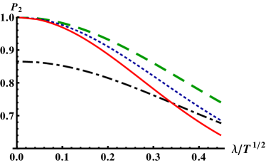
Figure 1: (Color online) Probability $P_{2}$ to end in the excited state at time $T$ versus noise parameter $\lambda$. Optimal protocol (green, dashed line), flat $\pi$-pulse with purely real Rabi frequency (blue, dotted line), pure adiabatic (black, dashed-dotted line), transitionless shortcut method (red, solid line). Additional parameter for adiabatic protocol and transitionless protocol: $\Omega_{0}T=5.57/4.3\,\pi$, $\delta_{0}T=(5.57/4.3)^{2}\pi$.

4.2 Example of a transitionless protocol

As another example, we will now look at the stability and noise sensitivity of a transitionless shortcut protocol. Our reference scheme is the finite-time sinusoidal model [33, 34]

$$\Omega_{R}(t)=\Omega_{0}\sin\left(\frac{\pi t}{T}\right)\,,\quad\Delta(t)=-\delta_{0}\cos\left(\frac{\pi t}{T}\right),$$ (47)

with $\Omega_{I}=0$ and $0\leq t\leq T$. The excitation probability is also shown in figure 1 (black, dashed-dotted line). The chosen intensities are not large enough and the population inversion is not complete.

Figure 1 shows the excitation probability also for the transitionless shortcut based on this sinusoidal model (red, solid line). The noise sensitivity of this protocol is $q_{N}=3.21/T$. Figure 2 shows the noise sensitivity for the transitionless protocol based on the sinusoidal model (47) for different values of $\delta_{0}$ and $\Omega_{0}$. The minimal noise sensitivity in this figure is achieved for $\delta_{0}=\Omega_{0}=0.5/T$ and it has the value $q_{N}=2.475/T$ which is very close to the noise sensitivity of the flat $\pi$ pulse in the previous subsection.

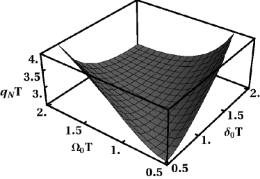
Figure 2: Noise sensitivity $q_{N}$ versus $\Omega_{0}$ and $\delta_{0}$ for the transitionless protocol.

4.3 Optimal scheme

We can also write the unperturbed Bloch vector in the form

$$\vec{r}_{0}(t)=\left(\begin{array}[]{c}\sin\Theta\cos\alpha\\ \sin\Theta\sin\alpha\\ \cos\Theta\end{array}\right).$$ (51)

This Bloch vector corresponds to the pure state in (24). Therefore we get from the Bloch equation the same equations (16). If the trajectory of the Bloch vector $\vec{r}(t)$ and $\Delta(t)$ is given, i.e. $\Theta,\alpha$ and $\Delta$ are given, then the corresponding $\Omega_{R}$ and $\Omega_{I}$ can be calculated by (30) and (31). Let $m(t)=\tan\Theta(\Delta+\dot{\alpha})$. Using (44), (51) and (30)-(32), we get for the noise error sensitivity

$$q_{N} = \frac{1}{4}\int_{0}^{T}dt\Big{[}(\cos^{2}\Theta+\cos^{2}\alpha\sin^{2}\Theta)(m\sin\alpha-\cos\alpha\dot{\Theta})^{2}$$ (53)

$$+(\cos^{2}\Theta+\sin^{2}\alpha\sin^{2}\Theta)(m\cos\alpha+\sin\alpha\dot{\Theta})^{2}\Big{]}\,\equiv\int_{0}^{T}dtL(m,\alpha,\Theta,\dot{\Theta}),$$

where $L$ is the Lagrange function for $q_{N}$. We are looking for functions $m(t),\Theta(t),\alpha(t)$ which minimize this functional. From the Euler-Lagrange formalism we get

$$0=\frac{\partial L}{\partial m}\Rightarrow m=\frac{\dot{\Theta}\sin(4\alpha)\sin^{2}\Theta}{4\cos^{2}\Theta+2\sin^{2}(2\alpha)\sin^{2}\Theta}.$$

Moreover

$$0=\frac{\partial L}{\partial\alpha}\Rightarrow\sin(4\alpha)=0\Rightarrow\alpha=n\pi/4.$$

From this it also follows that $m(t)=0$. Finally we have

$$0 = \frac{\partial L}{\partial\Theta}-\frac{d}{dt}\frac{\partial L}{\partial\dot{\Theta}}.$$ (54)

Let us now consider the cases $n$ odd and $n$ even separately.

Case $n$ even

If $n$ is even, then (54) simplifies to $\ddot{\Theta}=0$. Taking the boundary conditions $\Theta(0)=0,\Theta(T)=\pi$ into account, we arrive at

$$\Theta(t)=\pi t/T.$$

It follows that

$$\Omega_{R}=-\sin\left(\frac{n\pi}{4}\right)\,\frac{\pi}{T}\,,\quad\Omega_{I}=\cos\left(\frac{n\pi}{4}\right)\,\frac{\pi}{T}\,,\quad\Delta=0.$$

Note that either $\Omega_{R}$ or $\Omega_{I}$ is zero, so these schemes are flat $\pi$ pulses with a purely real or purely imaginary Rabi frequency. (As an example, we get for $n=6$ a $\pi$ pulse with a flat, real Rabi frequency $\Omega_{R}=\frac{\pi}{T}$ and $\Omega_{I}=0$.) For all these schemes an analytical solution of the master equation can be derived similar to the one in subsection 4.1 and the noise sensitivity of all schemes is $q_{N}=\pi^{2}/(4T)$.

Case $n$ odd

For $n$ odd we get

$$(3+\cos(2\Theta))\ddot{\Theta}=\sin(2\Theta)(\dot{\Theta})^{2}$$ (55)

Then $\Omega_{R}=\pm\dot{\Theta}/\sqrt{2}=\pm\Omega_{I}$ and $\Delta(t)=0$. We first solve (55) for $\Theta$ numerically and then put the solution in the expression for the noise sensitivity. The numerically calculated $\Theta(t)$ can be seen in figure 3 (solid line, left axis). The corresponding Rabi frequencies for $n=7$ are $\Omega_{R}(t)=\Omega_{I}(t)=\Omega(t)$, where $\Omega$ is shown also in figure 3 (dashed line, right axis). Note that for other values of odd $n$ only the signs of $\Omega_{R}$ resp. $\Omega_{I}$ are switched. The noise sensitivity value is $q_{N}=1.82424/T<\pi^{2}/(4T)$. Therefore, for $n$ odd, smaller noise sensitivities can be achieved than for $n$ even, so these protocols are least sensitive to amplitude noise. Finally, the optimal $\pi$ pulse is shown (green, dashed line) in figure 1, it has a noise sensitivity $q_{N}=1.82424/T$.

Note that an approximate solution of (55) is given by $\Theta(t)=\pi t/T-\frac{1}{12}\sin(2\pi t/T)$, with a noise sensitivity of $q_{N}=1.82538/T$.

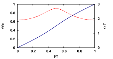
Figure 3: (Color online) Protocol with minimal noise sensitivity $q_{N}$, $\Theta(t)$ (blue, solid line; left axis), $\Omega(t)$ (red, dashed line; right axis).

5 Systematic errors

In this section we shall only consider systematic errors, i.e. $\lambda=0$. It is enough to work with pure states, instead of density matrices, satisfying the Schrödinger equation

$$i\hbar\frac{d}{dt}|\psi(t){\rangle}=(H_{0}(t)+\beta H_{1})|\psi(t){\rangle}.$$

We define the systematic error sensitivity as

$$q_{S}:=-\frac{1}{2}\left.\frac{\partial^{2}P_{2}}{\partial\beta^{2}}\right|_{\beta=0}=-\left.\frac{\partial P_{2}}{\partial(\beta^{2})}\right|_{\beta=0},$$

where $P_{2}$ is the probability to be in the excited state at final time $T$.

Using perturbation theory up to $O(\beta^{2})$ we get

$$|\psi(T){\rangle} = |\psi_{0}(T){\rangle}-\frac{i}{\hbar}\beta\int_{0}^{T}dt\hat{U}_{0}(T,t)H_{1}(t^{\prime})|\psi_{0}(t){\rangle}$$

$$-\frac{1}{\hbar^{2}}\beta^{2}\int_{0}^{T}dt\int_{0}^{t^{\prime}}dt^{\prime}\,\hat{U}_{0}(T,t)H_{1}(t^{\prime})\hat{U}_{0}(t,t^{\prime})H_{1}L_{1}(t^{\prime})|\psi_{0}(t^{\prime}){\rangle}+...,$$

where $|\psi_{0}(t){\rangle}$ is the unperturbed solution and $\hat{U}_{0}$ the unperturbed time evolution operator. We assume that the error-free ($\beta=0$) scheme works perfectly, i.e. $|\psi_{0}(T){\rangle}=e^{i\mu}|2{\rangle}$ with some real $\mu$. Then,

$$P_{2} = |{\langle}2|\psi(T){\rangle}|^{2}={\langle}\psi(T)|\psi_{0}(T){\rangle}{\langle}\psi_{0}(t)|\psi(T){\rangle}\approx 1-\frac{\beta^{2}}{\hbar^{2}}\left|\int_{0}^{T}dt{\langle}\psi_{\perp}(t)|H_{1}(t)|\psi_{0}(t){\rangle}\right|^{2}$$

because $\hat{U}_{0}(s,t)=|\psi_{0}(s){\rangle}{\langle}\psi_{0}(t)|+|\psi_{\perp}(s){\rangle}{\langle}\psi_{\perp}(t)|$, where ${\langle}\psi_{\perp}(t)|\psi_{0}(t){\rangle}=0$ for all times and $|\psi_{\perp}(t){\rangle}$ is also a solution of the Schrödinger equation, see (27). From this we get the systematic-error sensitivity value

$$q_{S} = \frac{1}{\hbar^{2}}\left|\int_{0}^{T}dt{\langle}\psi_{\perp}(t)|H_{1}(t)|\psi_{0}(t){\rangle}\right|^{2}.$$

5.1 Example: $\pi$ pulse

Let $\Delta=0$, $\Omega(t)=|\Omega(t)|e^{i\alpha}$ and $\int_{0}^{T}dt\,|\Omega(t)|=\pi$, which correspond to a $\pi$ pulse. Then we get that $H_{0}=H_{1}$ and an analytical solution exists,

$$P_{2} = \frac{1}{2}-\frac{1}{2}\cos\left((1+\beta)\int_{0}^{T}|\Omega(t^{\prime})|dt^{\prime}\right)=\frac{1}{2}-\frac{1}{2}\cos\left((1+\beta)\pi\right).$$

It follows that $q_{S}=\pi^{2}/4$ independently of the time duration $T$.

The excitation probability versus systematic noise $\beta$ is shown in figure 4. As an example we are looking at the $\pi$ pulse which was optimal for amplitude-noise error in the previous section (green, dashed line). It has the systematic-error sensitivity $q_{S}=\frac{\pi^{2}}{4}\approx 2.47$ which is equal for all $\pi$ pulses. Even if the protocol is maximally robust concerning amplitude-noise, it is very sensitive to systematic errors.

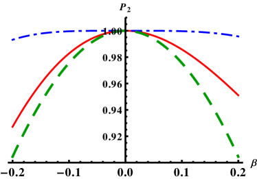
Figure 4: (Color online) Excitation probability $P_{2}$ versus systematic-error parameter $\beta$: protocol with zero systematic-error sensitivity (blue, dashed-dotted line), transitionless protocol (red, solid line), $\pi$ pulse with minimal noise sensitivity (green, dashed line).

5.2 Example of a transitionless shortcut

We again look at the example of a transitionless shortcut based on the sinusoidal model which was examined in subsection 4.2. The excitation probability versus systematic noise $\beta$ is shown in figure 4 (red solid line). The transitionless shortcut based on the sinusoidal model is more stable concerning systematic errors that any $\pi$ pulse.

Figure 5 shows the systematic-error sensitivity for the transitionless-based protocol for different values of $\delta_{0}$ and $\Omega_{0}$. Again, the protocol takes as a reference the sinusoidal model (47). Note that the systematic-error sensitivity $q_{S}$ for any $\pi$ pulse corresponds to the upper $x$-$y$ plane in this figure. This means that for all parameters shown the transitionless shortcut is less sensitive (i.e. more stable) concerning systematic error than any $\pi$ pulse.

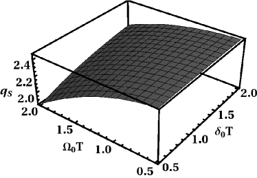
Figure 5: Systematic-error sensitivity $q_{S}$ versus $\Omega_{0}$ and $\delta_{0}$ for the transitionless protocol; the systematic-error sensitivity for a $\pi$ pulse corresponds to the upper $x$-$y$ plane.

5.3 Optimal scheme

To find an optimal scheme we shall use the invariant based technique. The pure state $|\psi(t){\rangle}$ can be parameterized as in (24). The boundary values should be $\Theta(0)=0$ and $\Theta(T)=\pi$. We get for the functions in the Hamiltonian leading to this solution

$$\Omega_{R} = \cos\alpha\sin\Theta\;\dot{\gamma}-\sin\alpha\;\dot{\Theta}$$

$$\Omega_{I} = \sin\alpha\sin\Theta\;\dot{\gamma}+\cos\alpha\;\dot{\Theta}$$

$$\Delta = -\cos\Theta\;\dot{\gamma}-\dot{\alpha}$$

Note that, contrary to section 4, it is now more convenient to take $\gamma(t)$ as a given function instead of $\Delta(t)$. A solution which is orthogonal to (24), i.e. ${\langle}\psi_{\perp}|\psi{\rangle}=0$ for all times, is given by (27). The expression for the systematic error sensitivity is now

$$q_{S} = \left|\int_{0}^{T}dt{\langle}\Psi_{\perp}(t)|H_{1}(t)/\hbar|\psi(t){\rangle}\right|^{2}$$

$$= \frac{1}{4}\left|\int_{0}^{T}dt\left[-ie^{-i\gamma}\dot{\gamma}\;\cos\Theta\sin\Theta+e^{-i\gamma}\dot{\Theta}\right]\right|^{2}$$

$$= \frac{1}{4}\left|\int_{0}^{T}dt\left[e^{-i\gamma}\;\frac{d}{dt}(\cos\Theta\sin\Theta)+e^{-i\gamma}\dot{\Theta}\right]\right|^{2},$$

where we have applied partial integration in the last step taking into account the boundary values $\Theta(0)=0$ and $\Theta(T)=\pi$. The expression can be further simplified and we get finally

$$q_{S} = \left|\int_{0}^{T}dte^{-i\gamma}\dot{\Theta}\sin^{2}\Theta\right|^{2}.$$

In the special case when $\gamma(t)$ is constant in time, we get $q_{S}=\frac{\pi^{2}}{4}$ independently of $\Theta(t)$. With the choice $\alpha(t)$ constant we recover the $\pi$ pulse.

The minimum of $q_{S}$ is clearly achieved if $q_{S}=0$. In the following we will show that there are protocols which fulfill this condition, i.e. protocols maximally stable with respect to systematic errors. We will give an example class which fulfills $q_{S}=0$. Let

$$\gamma(t)=n\left(2\Theta-\sin(2\Theta)\right).$$

For this choice of $\gamma$ we get

$$q_{S}=\frac{\sin^{2}\left(n\pi\right)}{4n^{2}}.$$

So for $n=1,2,3,...$ we get protocols fulfilling $q_{S}=0$. Note that in the limit of $n\to 0$ (i.e. $\gamma\to 0$), we get $q_{S}\to\frac{\pi^{2}}{4}$, which is consistent with the previous paragraph. The functions in the Hamiltonian in this case are

$$\Omega_{R} = \left(4n\cos\alpha\sin^{3}\Theta-\sin\alpha\right)\;\dot{\Theta},$$

$$\Omega_{I} = \left(4n\sin\alpha\sin^{3}\Theta+\cos\alpha\right)\;\dot{\Theta},$$

$$\Delta = -4n\cos\Theta\sin^{2}\Theta-\dot{\alpha}.$$

Note that this class of protocols might not be the only ones fulfilling $q_{S}=0$. There is still some freedom left. For example, one could in addition require that $\Delta=0$ or $\Omega_{I}=0$. In the following we will look at the second condition, i.e. $\Omega_{I}=0$ for all $t$. This leads to $\alpha(t)=-\mbox{arccot}\left(4n\sin^{3}\Theta\right)$. In addition, there is the freedom to chose $\Theta(t)$ with $\Theta(0)=0,\Theta(t_{f})=\pi$. For $n=1$ and $\Theta(t)=\pi t/t_{f}$, the resulting Rabi frequency and the detuning are shown in figure 6.

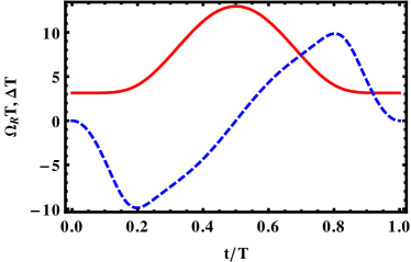
Figure 6: (Color online) Rabi frequency $\Omega_{R}$ (red, solid line) and detuning $\Delta$ (blue, dashed line) for a protocol which has zero systematic-error sensitivity.

6 Systematic and amplitude-noise errors

Finally, we will consider both types of errors together. Optimal schemes in this case would depend on the ratio between amplitude-noise error and systematic error in the experiment. We will just examine numerically the behavior of some protocols with respect to amplitude-noise and systematic error. Specifically we compare the minimal noise error protocol, the minimal systematic error protocol, and the example of a transitionless shortcut studied before, see figure 7. The figure shows that the different optimal schemes perform better than the other one depending on the dominance of one or the other type of error.

(a)

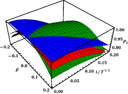
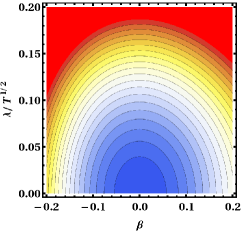
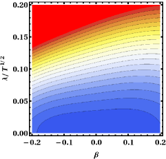
(b)  (c)  (d)

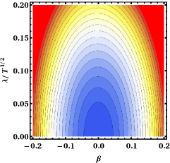
Figure 7: (Color online) Probability $P_{2}$ versus noise error and systematic error parameter; (a) transitionless protocol (red), optimal systematic stability protocol (blue), optimal noise protocol (green); same result as contour plots: (b) transitionless protocol, (c) optimal systematic stability protocol, (d) optimal noise stability protocol.

Summarizing, in this paper we have examined the stability of different fast protocols for exciting a two-level system with respect to amplitude-noise error and systematic errors. First we have looked at the noise error alone and we have introduced a noise sensitivity. We have shown that a special type of $\pi$ pulse is the optimal protocol with minimal noise sensitivity. Then we have looked at the systematic error alone and we have introduced a systematic error sensitivity. We have shown that there are protocols for which this sensitivity is exactly zero. Finally, we have looked at the general case with noise and systematic errors together.

Future work may involve extending the present results to different types of noise and perturbations. The existence of a set of optimal solutions for systematic errors also opens the way to further optimization with respect to other variables of physical interest.

Appendix A Derivation of the Master equation for Amplitude-Noise Error

The evolution of the quantum state with amplitude noise can only be described by a master equation [35]. We assume that the Hamiltonian has a deterministic part $H_{01}$ and a stochastic part containing $\lambda H_{2}$. We need a mapping from a fixed time to another infinitesimally close, so our starting point will be

$$|\psi_{t+dt}\rangle=e^{-i(H_{01}dt+\lambda H_{2}dW_{t})}|\psi_{t}\rangle$$ (56)

where $dt$ is the infinitesimal time step and $dW_{t}$ the corresponding noise increment in the Ito sense. The properties of such noise are: ${\langle}dW{\rangle}=0,{\langle}dW^{2}{\rangle}=dt$. If we expand in Taylor series (56) and keep terms up to first order in $dt$ and $dW$ (using the Ito calculus rules) we arrive at the following Stochastic Schrödinger equation (SSE)

$$|d\psi\rangle=-\frac{i}{\hbar}H_{01}dt|\psi\rangle-\frac{\lambda^{2}}{2\hbar^{2}}H_{2}^{2}dt|\psi\rangle-\frac{i\lambda}{\hbar}H_{2}dW_{t}|\psi\rangle.$$ (57)

The master equation derived from this SSE is then (33).

An equivalent approach in the Stratonovich sense is to start from

$$i\hbar\frac{d}{dt}\psi(t)=\left(H_{01}+\lambda H_{2}\underbrace{\frac{dW_{t}}{dt}}_{\xi(t)}\right)\psi(t),$$

where $\xi(t)$ is heuristically the time-derivative of the Brownian motion $W_{t}$. We have ${\langle}\xi(t){\rangle}=0$ and ${\langle}\xi(t)\xi(t^{\prime}){\rangle}\,=\delta(t-t^{\prime})$ because the noise should have zero mean and the noise at different times should be uncorrelated. If we average over different realizations and define $\rho(t)={\langle}\rho_{\xi}{\rangle}$ then $\rho(t)$ is fulfilling (33). To show this we define $\rho_{\xi}(t)=|\psi_{\xi}(t){\rangle}{\langle}\psi_{\xi}(t)|$. We start from the dynamical equation for $\rho_{\xi}$, namely

$$\frac{d}{dt}\rho_{\xi}=-\frac{i}{\hbar}[H_{01},\rho_{\xi}]-\frac{i\lambda}{\hbar}[H_{2},\xi\rho_{\xi}],$$ (58)

that after averaging over the noise becomes

$$\frac{d}{dt}\rho=-\frac{i}{\hbar}[H_{01},\rho]-\frac{i\lambda}{\hbar}[H_{2},{\langle}\xi\rho_{\xi}{\rangle}].$$ (59)

Novikov’s theorem applied to white noise takes the form

$${\langle}\xi(t)F[\xi]{\rangle}=\frac{1}{2}\left<\frac{\delta F}{\delta\xi(s)}\right>_{s=t}.$$

Using it we get

$${\langle}\xi\rho_{\xi}{\rangle}=-\frac{i\lambda}{2\hbar}[H_{2},\rho],$$ (60)

which leads to (33).

References

[1] Allen L and Eberly J H 1987 Optical Resonance and Two-level Atoms (New York: Dover)
[2] Vitanov N V, Halfmann T, Shore B W and Bergmann K 2001 Annu. Rev. Phys. Chem.52 763
[3] Bergmann K, Theuer H and Shore B W 1998 Rev. Mod. Phys.70 1003
[4] Král P, Thanopulos I and Shapiro M 2007 Rev. Mod. Phys.79 53
[5] Levitt M 1986 Prog. Nucl. Magn. Reson. Spectrosc.18 61
[6] Collin E, Ithier G, Aassime A, Joyez P, Vion D and Esteve D 2004 Phys. Rev. Lett.93 157005
[7] Torosov B T, Guérin S and Vitanov N V 2011 Phys. Rev. Lett.106 233001
[8]Demirplak M and Rice S A 2003 J. Phys. Chem. A107 9937; 2005 J. Phys. Chem. B109 6838; 2008 J. Chem. Phys.129 154111
[9] Berry M V 2009 J. Phys. A42 365303
[10] Chen X, Lizuain I, Ruschhaupt A, Guéry-Odelin D and Muga J G
2010 Phys. Rev. Lett.105 123003
[11] Masuda S and Nakamura K 2010 Proc. R. Soc. A466 1135; 2011 Phys. Rev. A84 043434
[12] Muga J G, Chen X, Ibáñez S, Lizuain I and Ruschhaupt A 2010
J. Phys. B: At. Mol. Opt. Phys.43 085509
[13] Chen X, Torrontegui E and Muga J G 2011
Phys. Rev. A83 062116
[14] Ibáñez S, Martínez-Garaot S, Chen X, Torrontegui E and Muga J G 2011 Phys. Rev. A84 023415
[15] Bason M G, Viteau M, Malossi N, Huillery P, Arimondo E, Ciampini D, Fazio R, Giovannetti V, Mannella R and Morsch O 2012 Nat. Phys.8
147
[16] Ibáñez S, Chen X, Torrontegui E, Ruschhaupt A and Muga
2011 J G arXiv:1112.5522
[17] Fasihi M A, Wan Y D and Nakahara M 2011 arXiv.1110.6707.
[18] Lacour X, Guérin S and Jauslin H R 2008 Phys. Rev. A78 033417
[19]Lewis H R and Riesenfeld W B 1969 J. Math. Phys.10 1458
[20]Muga J G, Chen X, Ruschhaupt A and Guéry-Odelin D
2009 J. Phys. B: At. Mol. Opt. Phys.42 241001
[21] Chen X, Ruschhaupt A, Schmidt S, del Campo A, Guéry-Odelin D and Muga J G 2010 Phys. Rev. Lett.104 063002
[22] Chen X and Muga J G 2010 Phys. Rev. A82 053403
[23] Stenfanatos D, Ruths H, Li J S 2010 Phys. Rev. A82 063422
[24] Schaff J F, X.-L. Song, P. Vignolo, and G. Labeyrie, Phys. Rev. A 82, 033430 (2010).
[25] Schaff J F, Song X L, Capuzzi P, Vignolo P and Labeyrie G 2011
EPL93 23001
[26] Schaff J F, Capuzzi P, Labeyrie G and Vignolo P
2011 New J. Phys.13 113017
[27] Torrontegui E, Ibáñez S, Chen X, Ruschhaupt A, Guéry-Odelin D and J. G. Muga J G 2011 Phys. Rev. A83 013415
[28] Torrontegui E, Chen X, Modugno M, Schmidt S, Ruschhaupt
A and Muga J G 2012
New J. Phys.14 013031
[29] Chen X, Torrontegui E, Stefanatos D, Li J S and Muga J G
2011 Phys. Rev. A84 043415
[30]Li Y, Wu L A and Wang Z D 2011 Phys. Rev. A83 043804
[31] del Campo A 2011 Phys. Rev. A84 031606(R);
2011 EPL96 60005
[32] Choi S, Onofrio R and Sundaram B 2011
Phys. Rev. A84 051601(R)
[33] Lu T, X. Miao X, and H. Metcalf H 2007 Phys. Rev. A75 063422;
Lu T S 2011 Phys. Rev. A84 033411
[34] Miao X, Wertz E, Cohen M G, and H. Metcalf H 2007
Phys. Rev. A75 011402(R)
[35] Carmichael H J 1999 Statistical methods in quantum optics 1
(Springer)
(c)
(c) (d)
(d)