Monte Carlo estimates of thermal averages and analytic continuation

Abstract

The Monte Carlo (MC) estimates of thermal averages are usually functions of system control parameters $\lambda$, such as temperature, volume, interaction couplings, etc. Given the MC average at a set of prescribed control parameters $\lambda_{0}$, the problem of analytic continuation of the MC data to $\lambda$-values in the neighborhood of $\lambda_{0}$ is considered in both classic and quantum domains. The key result is the theorem that links the differential properties of thermal averages to the higher-order cumulants. The theorem and analytic continuation formulas expressed via higher-order cumulants are numerically tested on the classical Lennard-Jones cluster system of $N=13$, 55, and 147 neon particles.

I Introduction

To obtain Monte Carlo (MC) estimates of thermal averages, one often has to run MC codes multiple times in order to get the corresponding results at different values of system parameters, such as temperature, volume, magnetic or electric fields, etc., or at different values of interparticle interaction constants. To avoid these extra time-consuming runs, several highly effective strategies for sampling phase space of the system and/or extracting maximum relevant information from the MC data acquired have been suggested. Among them, these are histogram methods by Ferrenberg and Swendsen FS:88 ; FS:89 , the multicanonical method by Berg and Neuhaus BN:91 ; BN:92 , the Wang-Landau method WL:01 and others.

Thus, in the first method we record a histogram $n(E)$ of how many times each particular value of the energy $E$ is generated in MC simulation at a particular temperature $T_{0}$. Then, using this energy distribution histogram one can in principle recalculate the corresponding energy distribution and thermal averages at an arbitrary temperature $T$. The multicanonical method is based on the idea of using inverse of the density of states, $1/\rho(E)$, instead of the Boltzmann factor $\exp(-\beta E)$, where $\beta=1/(k_{B}T)$ and $k_{B}$ is the Boltzmann constant, for sampling the energy states in the metastable-unstable region of the canonical ensemble. This results in a histogram in which all energies are sampled equally. The obvious problem with the direct implementation of this idea is that we do not know the density of states $\rho(E)$. However, using a sequence of approximations, Berg and Neuhaus were able to demonstrate that $\rho(E)$ can be found, even in a particularly impressive case of a first-order phase transition BN:92 . On the other hand, the Wang-Landau algorithm allows to estimate the density of states $\rho(E)$ directly instead of trying to estimate it from the probability distribution obtained at $T_{0}$ and then with density of states one can easily calculate the partition function, free energy, etc. at an arbitrary temperature $T$. Moreover, the original Wang-Landau algorithm WL:01 proposed for MC sampling in spin lattice systems has been generalized to the off-lattice systems, such as continuum (fluid) models SDP:02 ; YP:03 , polymer films JP:02 . By a suitable reformulation of the problem the Wang-Landau sampling scheme can be advantageously employed in quantum systems as well TWA:03 .

However, it should be noticed that the applicability of these methods is severely restricted by the presence of statistical errors in the data, $n(E)$ or $\rho(E)$, generated in MC sampling. If errors in the data become comparable or bigger than the true values in the energy range near the average potential energy at temperature $T$, then the above methods fail to continue the corresponding thermal averages from $T_{0}$ to $T$ temperatures.

In statistical physics, quantum mechanics, quantum field theory, and many other fields of modern theoretical physics, where some kind of averaging of a generalized exponential function is present, we constantly face the so-called cumulant expansions Gol:92 ; Ful:95 ; AS:06 . Although cumulants (semi-invariants) have been known long before in mathematical statistics and probability theory, it was Kubo who first convincingly demonstrated in his pioneering work Ku:62 how the concept of cumulants can be widely applied to various problems of quantum mechanics and statistical physics. For example, it has been successfully applied to Ursell-Mayer expansion for classical and quantum gases MM:40 that is usually obtained by much longer diagram considerations, to perturbation series in quantum mechanics and random perturbations in dynamical systems, to relaxation functions in irreversible processes Ku:57 ; Ku:62 , etc. In spite of such a diversity of applications discovered so far, cumulants and their properties have not been, to the best of our knowledge, exploited before in the context of analytic continuation problems both in classical and quantum domains. In his original paper, Kubo greatly generalized the classical concept of cumulant expansion to the case of non-commuting operator generating algebra and applied relations found in this algebra to a diverse set of physical problems. In KF:98 , a number of useful algebraic and geometric properties of cumulant expansions have been summarized and applied to generate cumulant Faddeev-like equations and to establish a method of increments for excited states. Very recently, cumulant expansion techniques have been successfully applied to the Fourier path integrals KFD:10 ; KFD:09 ; PKF:12 However, application of cumulants to the problem of analytic continuation requires the knowledge of differential properties of cumulants. These properties have not been established before. Therefore, one of the goals of the present paper is to derive those properties of cumulants that are of paramount importance for analytic continuation applications.

In this work, we present a new, more robust cumulant expansion method which allows to analytically continue thermal averages in the neighborhood of $T_{0}$. In particular, we prove the key Theorem IV.1 which relates the derivative of the $k$th order cumulant with respect to the inverse temperature $\beta$ to a $(k+1)$th order cumulant. Based on this theorem, one can develop an asymptotic expansion in the neighborhood of $T_{0}$ in terms of higher order cumulants. Also, some numerical results for the heat capacity of the Lennard-Jones (LJ) clusters illustrating the cumulant’s derivative theorem and the quality of the derived expansions are presented. One of the advantages of the proposed method is that the analytic continuation can be implemented directly without need of separate calculating $n(E)$ or $\rho(E)$ distributions. Moreover, given the cumulants, if necessary one can easily express these distributions in terms of cumulants.

The rest of the paper is organized as follows. The energy representation for the phase-space probability density function (pdf) is introduced in Section II. In the energy representation, all degrees of freedom irrelevant to thermodynamic equilibrium are integrated out. Next Section considers how partition function, entropy, and statistical temperature can be expressed via kinetic and potential energy pdfs. The thermodynamic energy, heat capacity and its differential properties are given in terms of cumulant expansions in Section IV. Here, the key Theorem IV.1 about cumulant’s derivative is formulated. In Section V, the cumulant expansions and the corresponding analytic continuation formula for the energy pdf are analyzed. The statistical or microcanonical temperature in terms of cumulants is analyzed in Section VI. Further generalizations to the multi-parameter classic and quantum systems are developed in Sections VII and VIII. Here, Theorem VII.1, a multi-parameter generalization of the Theorem IV.1 is formulated. Numerical results are discussed in Section IX. Concluding remarks are in Section X. Finally, technical details about cumulants, proofs of Theorems IV.1 and VII.1 can be found in Appendices A-C.

II Phase space to energy space mapping

Let us consider a classical system, the phase space of which is described by a set $\Omega$ of $3N$ canonically conjugate coordinate $\mathbf{r}=(\mathbf{r}_{1},\ldots,\mathbf{r}_{N})$ and$\ 3N$ momentum $\mathbf{p}=(\mathbf{p}_{1},\ldots,\mathbf{p}_{N})$ variables. On the phase space we define the pdf $p(\Omega)$ that fully describes a thermal equilibrium state such that the thermal average of an observable $\mathcal{O}(\Omega)$ can be calculated as

$$\langle\mathcal{O}(\Omega)\rangle\equiv\int d^{6N}\Omega\,\mathcal{O}(\Omega)p(\Omega)$$ (1)

where $d^{6N}\Omega=d^{3N}\mathbf{r}d^{3N}\mathbf{p}/w_{N}$ and $w_{N}$ is an appropriate weight factor, sometimes called Gibbs factor, which makes the classical averaging as close as possible to the quantum-mechanical one. Further, we assume that the pdf depends on $K$ functions $H(\Omega)\equiv(H_{1}(\Omega),\ldots,H_{K}(\Omega))$ and $K$ control parameters $\lambda\equiv(\lambda_{1},\ldots,\lambda_{K})$ so that its $\Omega$-dependence can be represented as $p(\Omega)=p(H(\Omega),\lambda)$ For the observable we assume a similar structure, $\mathcal{O}(\Omega)=\mathcal{O}(H(\Omega)),$ to be valid. If we define the $K$-dimensional energy pdf as

$$p(E,\lambda)=\int d^{6N}\Omega\prod\limits_{k=1}^{K}\delta(E_{k}-H_{k}(\Omega))p(H(\Omega),\lambda)$$ (2)

where $E\equiv(E_{1},\ldots,E_{K})$, then, the thermal averages can be be evaluated by integration in the energy space only

$$\langle\mathcal{O}(E)\rangle=\int d^{K}E\,\mathcal{O}(E)p(E,\lambda)$$ (3)

The original problem of integration in a $6N$-dimensional phase space is, thus, reduced to a $K$-dimensional integration in the energy space. In Eq. (2), we effectively integrated out all extra degrees of freedom not important in the equilibrium state.

The problem that now can be formulated is how to calculate this energy pdf at a fixed set of parameters. The energy pdf at an arbitrary set of parameters $\lambda$ can be calculated, at least in principle, if it is known at a fixed one, $\lambda_{0}$, as follows. Usually, the pdf in the phase space is known up to the normalization factor or partition function. We assume a generic form for

$$p=\exp\left(-\lambda\cdot H(\Omega)\right)/\mathcal{Z}(\lambda)$$ (4)

where $\cdot$ denotes the scalar product and the partition function

$$\mathcal{Z}(\lambda)=\int d^{6N}\Omega\,\exp\left(-\lambda\cdot H(\Omega)\right)$$ (5)

It assumes the existence of the partition function.

Using Metropolis et al. importance sampling algorithm MRR:53 ; LB:05 , for which there is no need a priori to know the partition function, one can evaluate the integral over $\Omega$ by the Markov chain MC simulation method and get a statistical estimate for the energy pdf $p(E,\lambda_{0})$ at $\lambda_{0}$ parameters. To this end, one can use a proper asymptotic representation for the $\delta$-functions in the integrand of Eq. (2)

$$\delta(E_{k}-H_{k})=\frac{1}{\pi}\lim\limits_{\tau\longrightarrow\infty}\frac{\sin\left(\tau(E_{k}-H_{k})\right)}{E_{k}-H_{k}}.$$ (6)

Having obtained the energy pdf at a fixed value $\lambda_{0}$, one can easily recalculate the pdf at an arbitrary value $\lambda$ using the formula

$$p(E,\lambda)=\dfrac{\exp\left(-(\lambda-\lambda_{0})\cdot E\right)p(E,\lambda_{0})}{\mathcal{Z}(\lambda,\lambda_{0})}$$ (7)

where the normalization factor

$$\mathcal{Z}(\lambda,\lambda_{0}) = \int d^{K}E\,\exp\left(-(\lambda-\lambda_{0})\cdot E\right)p(E,\lambda_{0})$$ (8)

$$= \frac{\mathcal{Z}(\lambda)}{\mathcal{Z}(\lambda_{0})}$$

is the ratio of partition functions calculated at $\lambda$ and $\lambda_{0}$ parameters. Thus, the thermal averages at arbitrary values of $\lambda$ can be evaluated with the help of Eqs. (3) and (7). Examples of such calculations in the system of particles interacting via LJ potential will be presented in Section IX.

III Classical partition function, density of states and statistical temperature

At first sight, the best one can get from Eq. (8) is the ratio of partition functions, not an absolute value at a particular set of parameters. However, at $\lambda=0$ the partition function takes an especially simple value: $\mathcal{Z}(0)=\int d^{6N}\Omega=V_{\Omega}/w_{N},$ where $V_{\Omega}$ is the total available volume of the phase space. In classical, non-relativistic physics $V_{\Omega}$ is, in principle, infinite due to possible infinite particle’s momentum values. However, it is well known LL:80 that kinetic energy contribution to the partition function, $\mathcal{Z}_{\mathcal{K}}(\beta)$, where $\beta$ is the inverse temperature, can be evaluated exactly and calculation of the partition function, $\mathcal{Z}_{\mathcal{K}+\mathcal{V}}(\lambda)\equiv\mathcal{Z}_{\mathcal{K}}(\beta)\mathcal{Z}_{\mathcal{V}}(\lambda),$ is, thus, reduced to the computation of the configuration integral, $\mathcal{Z}_{\mathcal{V}}(\lambda)$, defined as in Eq. (5), where $\Omega\rightarrow\mathbf{r}$ is a position in the configuration space and $H(\Omega)$ is replaced by the potential energy $\mathcal{V}(\mathbf{r})$.

Therefore, the configuration integral

$$\mathcal{Z}_{\mathcal{V}}(0)=V^{N},$$ (9)

where $V$ is the spatial volume of the system. From Eq. (8), we find that

$$\mathcal{Z}_{\mathcal{V}}(\lambda)=V^{N}\frac{\int d^{K}E\,\exp\left(-(\lambda-\lambda_{0})\cdot E\right)p_{\mathcal{V}}(E,\lambda_{0})}{\int d^{K}E\,\exp\left(\lambda_{0}\cdot E\right)p_{\mathcal{V}}(E,\lambda_{0})}$$ (10)

Here, $p_{\mathcal{V}}(E,\lambda_{0})$ is the potential energy pdf. Notice that at $\lambda=\lambda_{0}$, the integral in the numerator is equal to one due to normalization of the pdf, whereas at $\lambda=0$, Eq. (10) is reduced to (9).

As an example, let us consider the case of a single parameter $\lambda_{01}=\beta_{0}=1/(k_{B}T_{0})$, where $T_{0}$ is an absolute temperature, $\ \mathcal{V}_{1}(\mathbf{r})=\mathcal{V}(\mathbf{r})$ is the potential energy. We wish to calculate the density of states

$$\rho_{\mathcal{K}+\mathcal{V}}(E)\equiv\int d^{6N}\Omega\,\delta(E-\mathcal{K}(\mathbf{p})-\mathcal{V}(\mathbf{r}))$$ (11)

In contrast to the partition function, the calculation of the density of states cannot be factorized in separate integrals over momenta and coordinates. To overcome this difficulty, it is useful first to map the phase space to the two-dimensional energy space as suggested by Eq. (2), namely, to define the 2$D$ pdf in a factorized form

$$p_{\mathcal{K},\mathcal{V}}(E_{1},E_{2},\beta_{0})= p_{\mathcal{K}}(E_{1},\beta_{0})p_{\mathcal{V}}(E_{2},\beta_{0}),$$ (12)

$$p_{\mathcal{K}}(E_{1},\beta_{0})= \int d^{3N}\mathbf{p}\,\delta(E_{1}-\mathcal{K}(\mathbf{p}))\dfrac{\exp(-\beta_{0}\mathcal{K}(\mathbf{p}))}{\mathcal{Z}_{\mathcal{K}}(\beta_{0})}$$

$$p_{\mathcal{V}}(E_{2},\beta_{0})= \int d^{3N}\mathbf{r}\,\delta(E_{2}-\mathcal{V}(\mathbf{r}))\dfrac{\exp(-\beta_{0}\mathcal{V}(\mathbf{r}))}{\mathcal{Z}_{\mathcal{V}}(\beta_{0})}$$

Similar to the kinetic energy partition function, the pdf $p_{\mathcal{K}}$ can be calculated exactly; see, e.g., Ka:00 , Ch. 3.

With the 2$D$ energy pdf (12), Eq.(11) can be rewritten as a convolution of the kinetic and potential energy pdfs

$$\rho_{\mathcal{K}+\mathcal{V}}(E) = \mathcal{Z}_{\mathcal{K}+\mathcal{V}}(\beta_{0})\exp(\beta_{0}E)$$ (13)

$$\times \int dE_{2}\,p_{\mathcal{K}}(E-E_{2},\beta_{0})p_{\mathcal{V}}(E_{2},\beta_{0})$$

Substituting explicit expressions for $\mathcal{Z}_{\mathcal{K}+\mathcal{V}}$ and $p_{\mathcal{K}}$ into (13), one obtains

$$\rho_{\mathcal{K}+\mathcal{V}}(E)=\dfrac{V^{N}(2\pi m)^{\frac{3N}{2}}}{\Gamma(\frac{3N}{2})}$$ (14)

$$\times \dfrac{\int\limits_{-\infty}^{E}dE_{2}\,(E-E_{2})^{\frac{3N}{2}-1}\exp(\beta_{0}E_{2})p_{\mathcal{V}}(E_{2},\beta_{0})}{\int\limits_{-\infty}^{\infty}dE_{2}\,\exp(\beta_{0}E_{2})p_{\mathcal{V}}(E_{2},\beta_{0})},$$

where $m$ is particle’s mass and $\Gamma(\frac{3N}{2})$ the Gamma function AS:72 , expressed in terms of the potential energy pdf. In the limiting case of zero interaction, $\mathcal{V}(\mathbf{r})\equiv 0$, $p_{\mathcal{V}\to 0}(E)\to\delta(E)$ is reduced to a $\delta$-function and the density of states Eq. (14) is defined only by the kinetic energy contribution, $\rho_{\mathcal{K}}(E)=\theta(E)V^{N}(2\pi m)^{3N/2}E^{3N/2-1}/\Gamma(3N/2)$, where $\theta(E)$ is the Heaviside step function. It is easy to check this result directly from Eq. (11).

Moreover, from Eq. (14) for the density of states we find the corresponding expressions for the entropy, $S_{\mathcal{K}+\mathcal{V}}(E)=k_{B}\ln\rho_{\mathcal{K}+\mathcal{V}}(E)$, and the statistical temperature

$$T_{\mathcal{K}+\mathcal{V}}(E) = \left(\frac{dS_{\mathcal{K}+\mathcal{V}}(E)}{dE}\right)^{-1}=\dfrac{g_{1}(E)}{k_{B}\left(\frac{3N}{2}-1\right)g_{2}(E)},$$ (15)

$$g_{p}(E) = \int\limits_{-\infty}^{E}dE_{2}\,(E-E_{2})^{\frac{3N}{2}-p}\exp(\beta_{0}E_{2})p_{\mathcal{V}}(E_{2},\beta_{0})$$ (16)

$$= \exp(\beta_{0}E)\int\limits_{0}^{\infty}dE_{1}E_{1}^{\frac{3N}{2}-p}\exp(-\beta_{0}E_{1})p_{\mathcal{V}}(E-E_{1},\beta_{0})$$

in terms of the potential energy pdf. If $\mathcal{V}\equiv 0$, then from Eq. (15) one gets for the kinetic energy temperature

$$T_{\mathcal{K}}(E)=\dfrac{\theta(E)E}{k_{B}\left(\frac{3N}{2}-1\right)}$$ (17)

Here, although formally $\rho_{\mathcal{K}}=0$ and $T_{\mathcal{K}}$ does not exist at $E<0$, we put $T_{\mathcal{K}}=0$ by a continuity at negative energies. Then, we can measure the potential energy contribution to the temperature as the difference $T_{\mathcal{V}}\equiv T_{\mathcal{K}+\mathcal{V}}-T_{\mathcal{K}}$.

IV Thermodynamic energy, heat capacity and cumulant expansion

The thermodynamic average of the energy written via the first moment or the first cumulant term reads as

$$U(\beta) = \frac{3N}{2\beta}+\mu_{c1}(\beta),$$ (18)

$$\mu_{c1}(\beta) = \mu_{1}(\beta)=\left\langle E\right\rangle_{p_{\mathcal{V}}(E,\beta)}=\left\langle V(\mathbf{r})\right\rangle_{p_{\mathcal{V}}(\mathbf{r},\beta)}$$ (19)

where the first and second terms are, respectively, due to the kinetic and potential energy contributions. Here, $\left\langle\ldots\right\rangle$ denote averages over the potential energy pdfs either in the energy or coordinate spaces.

Differentiating the $k$th-order moment $\mu_{k}(\beta)\equiv\left\langle E^{k}\right\rangle_{p_{\mathcal{V}}(E,\beta)}$ with respect to $\beta$, one obtains from the definition

$$\frac{d\mu_{k}}{d\beta}=-\mu_{k+1}+\mu_{k}\mu_{1}$$ (20)

The following theorem establishes a similar relationship between the derivative of the $k$th and $(k+1)$th cumulants.

Theorem IV.1

(univariate): Let $\mu_{ck}(\beta)$ be the $k$th-order classical cumulant. Then,

$$\frac{d\mu_{ck}}{d\beta}=-\mu_{c(k+1)}.$$ (21)

The general definition of the $k$th-order cumulant is given elsewhere, see, e.g., Ku:62 , and Appendix A. For proof of Theorem IV.1 we refer to Appendix B.

Using the relationship between the derivatives $d/dT=-k_{B}\beta^{2}d/d\beta$ and Eq. (21), one can easily find derivatives of energy (18) with respect to temperature expressed in terms of the second and higher-order cumulants. For example, for the first two derivatives we have

$$C_{V} = \dfrac{d\tilde{U}(T)}{dT}=-k_{B}\beta^{2}\dfrac{U(\beta)}{d\beta}=\frac{3}{2}Nk_{B}+k_{B}\beta^{2}\mu_{c2}(\beta),$$

$$\dfrac{dC_{V}}{dT} = \dfrac{d^{2}\tilde{U}(T)}{dT^{2}}=k_{B}^{2}\beta^{3}\left[-2\mu_{c2}(\beta)+\beta\mu_{c3}(\beta)\right]$$ (22)

From (22) one immediately derives that the extrema points of the heat capacity curve are defined by equation

$$2\mu_{c2}(\beta)=\beta\mu_{c3}(\beta)$$ (23)

Using Taylor’s series expansion near a fixed value $\beta_{0}$ and the equation for derivatives

$$\dfrac{d^{k}\mu_{cp}}{d\beta^{k}}=(-1)^{k}\mu_{c(p+k)},\quad p,k=1,2,3,\ldots$$ (24)

that follows from Theorem IV.1, Eq. (23) can be rewritten as

$$\sum_{k=0}^{\infty}\left[\beta_{0}\mu_{c(k+3)}(\beta_{0})-(k+1)\mu_{c(k+2)}(\beta_{0})\right]\dfrac{(-\Delta\beta)^{k}}{k!}=\mu_{c2}(\beta_{0})$$ (25)

where $\Delta\beta=\beta-\beta_{0}$. Solving this algebraic equation truncated at some maximum power $k=k_{max}$ for $\Delta\beta$, one obtains a converged root that can locate an extremum position.

Similarly, for the heat capacity one obtains the expansion

$$\dfrac{C_{V}}{k_{B}} = \frac{3}{2}N+\beta^{2}\left[\mu_{c2}(\beta_{0})-\mu_{c3}(\beta_{0})\Delta\beta\right.$$ (26)

$$+ \left.\frac{1}{2}\mu_{c4}(\beta_{0})\Delta\beta^{2}-\frac{1}{6}\mu_{c5}(\beta_{0})\Delta\beta^{3}+\cdots\right]$$

Some numerical applications of these equations will be given in Section IX.

V The energy pdf and cumulant expansion

Using the Fourier integral representation for $\delta$-function, we obtain an integral representation for

$$p_{\mathcal{V}}(E,T)=\frac{1}{2\pi}\int\limits_{-\infty}^{\infty}d\tau\exp\left(\mathrm{i}\tau E\right)\left\langle\exp\left(-\mathrm{i}\tau V(\mathbf{r})\right)\right\rangle_{p_{\mathcal{V}}(\mathbf{r},T)}$$ (27)

Formally, averaging the exponential function can be rewritten in terms of cumulant’s expansion as Ku:62

$$\left\langle\exp\left(-\mathrm{i}\tau V(\mathbf{r})\right)\right\rangle_{p_{\mathcal{V}}(\mathbf{r},T)} = \exp\left(\Xi_{c}(\tau,\beta)\right),$$ (28)

$$\Xi_{c}(\tau,\beta) = \sum\limits_{k=1}^{\infty}\frac{(-\mathrm{i}\tau)^{k}}{k!}\mu_{ck}(\beta)$$

where $\mu_{ck}$ is the $k$th cumulant. On the other hand, with the help of Taylor’s series expansion and Theorem IV.1, one obtains the following cumulant expansion for

$$\mu_{c1}(\beta+\mathrm{i}\tau) = \sum_{k=0}^{\infty}\dfrac{(\mathrm{i}\tau)^{k}}{k!}\dfrac{d^{k}\mu_{c1}(\beta)}{d\beta^{k}},$$ (29)

$$= \sum_{k=0}^{\infty}\dfrac{(-\mathrm{i}\tau)^{k}}{k!}\mu_{c(k+1)}(\beta)$$

Therefore, from (28) and (29) one derives alternative integral representations for

$$\Xi_{c}(\tau,\beta)=-\mathrm{i}\int_{0}^{\tau}d\tau^{\prime}\mu_{c1}(\beta+\mathrm{i}\tau^{\prime})$$ (30)

and

$$p_{\mathcal{V}}(E,T)=\frac{1}{2\pi}\int\limits_{-\infty}^{\infty}d\tau\exp\left(\mathrm{i}\tau E-\mathrm{i}\int_{0}^{\tau}d\tau^{\prime}\mu_{c1}(\beta+\mathrm{i}\tau^{\prime})\right)$$ (31)

Let us consider truncated cumulant expansions defined as

$$\Xi_{c}^{(k_{max})}(\tau,\beta)=\sum\limits_{k=1}^{k_{max}}\frac{(-\mathrm{i}\tau)^{k}}{k!}\mu_{ck}(\beta)$$ (32)

for the first $k_{max}=1,2,3$ values. Thus, at $k_{max}=1$ we easily get a $\delta$-function like pdf

$$p_{\mathcal{V}}^{(1)}=\delta(E-\mu_{c1}(\beta)),$$ (33)

while at $k_{max}=2$ integration over $\tau$ yields the Gaussian function

$$p_{\mathcal{V}}^{(2)}=\frac{1}{\sqrt{2\pi\mu_{c2}(\beta)}}\exp\left[-\frac{(E-\mu_{c1}(\beta))^{2}}{2\mu_{c2}(\beta)}\right].$$ (34)

The next case of $k_{max}=3$ is more complicated; the pdf is reduced to an Airy function. First, we have to shift the integration variable to the complex plane $\tau^{\prime}=\tau+\mathrm{i}\mu_{c2}/\mu_{c3}$ in order to cancel the quadratic term in the exponent

$$p_{\mathcal{V}}^{(3)} = \dfrac{1}{2\pi}\int\limits_{-\infty}^{\infty}d\tau\exp\left\{\mathrm{i}\tau(E-\mu_{c1})-\frac{\tau^{2}}{2}\mu_{c2}+\mathrm{i}\frac{\tau^{3}}{6}\mu_{c3}\right\}$$ (35)

$$= \dfrac{2^{1/3}\exp(\phi)}{2\pi\lvert\mu_{c3}\rvert^{1/3}}\int\limits_{-\infty+\mathrm{i}\mu_{c2}/\mu_{c3}}^{\infty+\mathrm{i}\mu_{c2}/\mu_{c3}}d\tau^{\prime}\exp\left\{\mathrm{i}\omega\tau^{\prime}+\mathrm{i}\frac{\tau^{\prime}{}^{3}}{3}\right\}$$

where

$$\phi = \frac{\mu_{c2}}{\mu_{c3}}(E-\mu_{c1})+\frac{\mu_{c2}^{3}}{3\mu_{c3}^{2}},$$

$$\omega = \dfrac{2^{1/3}\left(E-\mu_{c1}+\frac{\mu_{c2}^{2}}{2\mu_{c3}}\right)}{\mu_{c3}^{1/3}}$$ (36)

Let us consider a closed rectangular path $C=\bigcup_{i=1}^{4}C_{i}$ in the complex plane $\tau$ [see Fig. 1] consisting of two finite horizontal $C_{1}$ and $C_{3}$, and two vertical $C_{2}$ and $C_{4}$ segments. The horizontal segments are defined as $C_{1}=\left\{\tau:\,-t<\mathrm{{Re}\,\tau<t,\,{Im}\,\tau=\mu_{c2}/\mu_{c3}}\right\}$ and $C_{3}=\left\{\tau:\,-t<\mathrm{{Re}\,\tau<t,\,{Im}\,\tau=0}\right\}$, where $0<t<\infty$ is a parameter fixing the ends of segments, while the vertical segments $C_{2,4}=\left\{\tau:\,\mathrm{{Re}\,\tau=\pm t,\,0<{Im}\,\tau<\mu_{c2}/\mu_{c3}}\right\}$ connect the corresponding ends of the horizontal ones. Here, we have assumed that $C_{1}$ lies in the upper plane, i.e., $\mu_{c3}>0$; the negative case can be considered similarly. According to the Cauchy theorem, contour integral of a holomorphic function along a closed path is zero. Thus, we have $\oint_{C}d\tau\cdots=\sum_{i=1}^{4}\int_{C_{i}}d\tau\cdots=0$. It is easy to check that in the limit $t\rightarrow\infty$ contributions from the vertical segments go to zero and, therefore, integral along the real axis and the one taken along the path shifted into the complex plane turn out to be the same

$$\int\limits_{-\infty+\mathrm{i}\mu_{c2}/\mu_{c3}}^{\infty+\mathrm{i}\mu_{c2}/\mu_{c3}}d\tau\exp\left\{\mathrm{i}\omega\tau+\mathrm{i}\frac{\tau^{3}}{3}\right\}=\int\limits_{-\infty}^{\infty}d\tau\exp\left\{\mathrm{i}\omega\tau+\mathrm{i}\frac{\tau^{3}}{3}\right\}$$

and (35) in terms of Airy function takes the form

$$p_{\mathcal{V}}^{(3)}=\dfrac{2^{1/3}\exp(\phi)}{\lvert\mu_{c3}\rvert^{1/3}}\,\mathrm{{Ai}\,(\omega)}$$ (37)

Contrary to the $p_{\mathcal{V}}^{(2)}$ pdf, which is a symmetric distribution with respect to $\mu_{c1}$, $p_{\mathcal{V}}^{(3)}$ exhibits an asymmetric behavior. The Airy function shows qualitatively different behaviors: an oscillatory one at $\omega<0$, while an exponential decay at $\omega>0$. However, there is no guarantee that always $p_{\mathcal{V}}^{(3)}\geq 0$ because of possible oscillations at $\omega<0$.

One can see that the pdf $p_{\mathcal{V}}^{(k_{\max})}$ is not reducible to elementary functions at $k_{\max}=3$. Moreover, it is expected that in general $p_{\mathcal{V}}^{(k_{\max})}$ cannot be expressed via elementary functions at $k_{\max}>3$ as well. At $k_{\max}\geq 3$, the asymptotic saddle-point (SP) approximation Deb:09 can be applied in order to derive elementary working formulas. Thus, in the SP approximation, an integral

$$I_{k_{\max}}=\mathrm{Re}\int\limits_{-\infty}^{\infty}d\tau a(\tau)\exp\left(\Phi_{k_{\max}}(\tau)\right)$$ (38)

is estimated as

$$I_{k_{\max}}\sim\mathrm{Re}\sum_{\tau_{c}}a(\tau_{c})\sqrt{-\dfrac{2\pi}{\Phi_{k_{\max}}^{\prime\prime}(\tau_{c})}}\exp\left(\Phi_{k_{\max}}(\tau_{c})\right)$$ (39)

where $\Phi_{k_{\max}}\equiv\mathrm{i}\tau E+\Xi_{c}^{(k_{max})}(\tau,\beta)$ is a complex phase function truncated at $k_{\max}$ power and the critical points $\tau_{c}$ are solutions of the equation $\Phi_{k_{\max}}^{\prime}(\tau_{c})=0$.

At $k_{\max}=2$, the SP approximation reproduces the exact result (34). Let us apply Eq. (39) to the case of $k_{\max}=3$. We have the two critical points

$$\mathrm{i}\tau_{c\pm} = \dfrac{\mu_{c2}}{\mu_{c3}}\pm\sqrt{D},$$ (40)

$$D = \left(\dfrac{\mu_{c2}}{\mu_{c3}}\right)^{2}+\dfrac{2(E-\mu_{c1})}{\mu_{c3}}$$

The phase function $\Phi_{3}$ truncated at third power and its double derivative are reduced at these points to

$$\Phi_{3}({\tau_{c\pm}}) = \frac{\mu_{c2}}{2}D-\frac{1}{6}\frac{\mu_{c2}^{3}}{\mu_{c3}^{2}}\pm\frac{\mu_{c3}}{3}D^{3/2},$$ (41)

$$\Phi^{\prime\prime}_{3}(\tau_{c\pm}) = \pm\mu_{c3}\sqrt{D}$$

Substituting these equations into (39), one gets

$$p^{(3SP)}_{\mathcal{V}} = \mathrm{Re}\,\left\{\sqrt{\dfrac{1}{2\pi\mu_{c3}\sqrt{D}}}\exp\left(\dfrac{\mu_{c2}}{2}D-\dfrac{\mu_{c2}^{3}}{\mu_{c3}^{2}}\right)\right.$$ (42)

$$\times \left.\left[\mathrm{i}\exp\left(\dfrac{\mu_{c3}}{3}D^{3/2}\right)+\exp\left(-\dfrac{\mu_{c3}}{3}D^{3/2}\right)\right]\right\}$$

The SP approximation (42) is seen to have a $1/4$th power singularity at $D=0$ or at $E_{sing}=\mu_{c1}-\mu_{c2}^{2}/(2\mu_{c3})$. At the singularity point, where the two critical points coalesce, the standard SP approximation is not valid.

If the pdf $p_{\mathcal{V}}(\beta_{0})$ is known at a fixed value $\beta_{0}$, then its analytic continuation to $\beta=\beta_{0}+\Delta\beta$ point is given by

$$p_{\mathcal{V}}(E,\beta)=\dfrac{\exp\left(-\Delta\beta E\right)p_{\mathcal{V}}(E,\beta_{0})}{S(\Delta\beta,\beta_{0})}$$ (43)

where the normalization factor

$$S(\Delta\beta,\beta_{0})=\int dE\,\exp\left(-\Delta\beta E\right)p_{\mathcal{V}}(E,\beta_{0})$$ (44)

Let us calculate the normalization for the first three truncated pdfs, $p_{\mathcal{V}}^{(1,2,3)}$. One gets consecutively

$$S^{(1)} = \exp\left(-(\Delta\beta)\mu_{c1}(\beta_{0})\right),$$

$$S^{(2)} = \exp\left(-(\Delta\beta)\mu_{c1}(\beta_{0})+\frac{\mu_{c2}(\beta_{0})}{2}(\Delta\beta)^{2}\right),$$

$$S^{(3)} = \exp\left(-(\Delta\beta)\mu_{c1}(\beta_{0})+\frac{\mu_{c2}(\beta_{0})}{2}(\Delta\beta)^{2}-\frac{\mu_{c3}(\beta_{0})}{6}(\Delta\beta)^{3}\right)$$ (45)

where in the last line the Airy averaging has been carried out with the help of an integral formula VS:04

$$\int_{-\infty}^{\infty}dt\,\exp(pt)\mathrm{Ai}\,(t)=\exp(p^{3}/3),\quad\mathrm{Re}\,p>0.$$ (46)

If the average potential energy $\mu_{c1}$ is negative, then the normalization factor is exponentially small or large, depending on the sign of $\Delta\beta$. At $\Delta\beta>0$, $S$ is large or it is small otherwise.

Eqs. (45) suggest an anzatz for

$$S(\Delta\beta,\beta_{0}) = \exp\left(\kappa(\Delta\beta,\beta_{0})\right),$$

$$\kappa(\Delta\beta,\beta_{0}) = \sum_{k=1}^{\infty}c_{k}(\beta_{0})(\Delta\beta)^{k}$$ (47)

where the first three coefficients are defined by Eq. (45) as $c_{k}(\beta_{0})=(-1)^{k+1}\mu_{ck}(\beta_{0})/k!$, $k=1,2,3$. It can be easily checked that the same formula holds valid for the higher-order coefficients at $k>3$. It follows directly from equation

$$\mu_{c2}(\Delta\beta,\beta_{0}) = \dfrac{d^{2}S(\Delta\beta,\beta_{0})/d(\Delta\beta)^{2}}{S(\Delta\beta,\beta_{0})}-\left(\dfrac{dS(\Delta\beta,\beta_{0})/d(\Delta\beta)}{S(\Delta\beta,\beta_{0})}\right)^{2}$$ (48)

$$= \dfrac{d^{2}\kappa(\Delta\beta,\beta_{0})}{d(\Delta\beta)^{2}}$$

as a result of equating the like powers in Taylor’s expansions for $\mu_{c2}(\Delta\beta,\beta_{0})$ [see Eq. (26)] and the second derivative of $\kappa(\Delta\beta,\beta_{0})$ in the right-hand side.

VI The Statistical Temperature and cumulant expansion

Making use of the integral representation Eq. (31), the statistical temperature in terms of cumulants can be rewritten as

$$T_{\mathcal{K+V}}(E) = \dfrac{f_{1}(E)}{k_{B}f_{2}(E)},$$ (49)

$$f_{p}(E) = \int_{-\infty}^{\infty}d\tau a_{p}(\tau)\exp(\Phi(\tau))$$ (50)

where

$$a_{p}(\tau) = (\beta_{0}+\mathrm{i}\tau)^{-\alpha_{p}},\quad\alpha_{p}=3N/2-p+1,$$

$$\Phi(\tau) = \mathrm{i}\tau E-\mathrm{i}\int_{0}^{\tau}d\tau^{\prime}\mu_{c1}(\beta_{0}+\mathrm{i}\tau^{\prime})$$ (51)

$$= \mathrm{i}\tau E+\sum\limits_{k=1}^{\infty}\frac{\mu_{ck}(\beta_{0})}{k!}(-\mathrm{i}\tau)^{k}$$

The second line in $\Phi(\tau)$ is due to Theorem IV.1. $f_{p}(E)$ can be written in an explicitly real form

$$f_{p}(E)=2\int_{0}^{\infty}d\tau\frac{\exp\left(g(\tau)\right)}{\left(\beta_{0}^{2}+\tau^{2}\right)^{\alpha_{p}/2}}\cos\left(\varphi(\tau)\right)$$ (52)

where

$$g(\tau) = \sum\limits_{s=1}^{\infty}\frac{\mu_{c(2s)}(\beta_{0})}{(2s)!}\left(-\tau^{2}\right)^{s},$$

$$\varphi(\tau) = E\tau-\sum\limits_{s=0}^{\infty}\frac{\mu_{c(2s+1)}(\beta_{0})}{(2s+1)!}(-1)^{s}\tau^{2s+1}-\alpha_{p}\arctan\frac{\tau}{\beta_{0}}$$ (53)

While the ’real’ form (52) might be convenient for numerical estimates of the integrals, the ’complex’ representation (50) is a good starting point for developing the SP approximations. The critical points $\tau_{c}$ are defined by

$$\sum_{k=0}^{k_{max}}\dfrac{\mu_{c(k+1)}(\beta_{0})}{k!}(-\mathrm{i}\tau_{c})^{k}=E$$ (54)

Solving Eq. (54) for $\tau_{c}$, one gets the critical points. In the simplest approximation, truncating equation at $k_{max}=1$, we find

$$\mathrm{i}\tau_{c}=-\dfrac{E-\mu_{c1}(\beta_{0})}{\mu_{c2}(\beta_{0})}.$$ (55)

Then, with the help of (39) one obtains an asymptotic estimate for the temperature

$$T_{\mathcal{K+V}}(E) = \dfrac{T_{0}}{1-\dfrac{k_{B}T_{0}(E-\mu_{c1}(\beta_{0}))}{\mu_{c2}(\beta_{0})}}$$ (56)

$$\approx T_{0}\left[1+\dfrac{k_{B}T_{0}(E-\mu_{c1}(\beta_{0}))}{\mu_{c2}(\beta_{0})}\right]$$

where the second line is valid if the ratio in the denominator taken by modulus is much less than one. In the neighborhood of $\mu_{c1}$, $T_{\mathcal{K+V}}$ is seen to grow linearly as $E$ increases. Notice that a similar piecewise linear interpolation scheme for the statistical temperature has been suggested in the statistical-temperature MC (STMC) and molecular dynamics (STMD) algorithms KSK:06 .

At $k_{max}=2$, solving the quadratic equation one obtains the two critical points (40). Substituting the phase function and its double derivative (51) taken at these points into (39), where $a(\tau)=(\beta_{0}+\mathrm{i}\tau)^{-\alpha_{p}}$, one gets

$$f_{p}(E)\sim\mathrm{Re}\,\sum_{\pm}\frac{1}{\left(\beta_{0}+\dfrac{\mu_{c2}}{\mu_{c3}}\pm\sqrt{D}\right)^{\alpha_{p}}}\sqrt{\frac{-1}{\pm\mu_{c3}\sqrt{D}}}\exp\left(\pm\frac{\mu_{c3}}{3}D^{3/2}\right)$$ (57)

Let us assume that $E$ is in the neighborhood of $\mu_{c1}$ such that $D>0$. Then, depending on the sign of $\mu_{c3}$, we find that one term in the sum (57) is real and the other purely imaginary. Thus, if $\mu_{c3}>0$, the ”$-$”-sign term is real, while the ”$+$”-sign term is imaginary. Taking into account only the real contributions to $f_{p}$, one obtains

$$T_{\mathcal{K+V}}(E) = \dfrac{1}{k_{B}\left(\beta_{0}+\dfrac{\mu_{c2}}{\mu_{c3}}-\mathrm{sign}\,(\mu_{c3})\sqrt{D}\right)}$$ (58)

where $\mathrm{sign}\,(x)=\pm 1$ if $x$ is positive or negative. Moreover, if

$$\left|\dfrac{2(E-\mu_{c1})}{\mu_{c3}}\right|\ll\left(\dfrac{\mu_{c2}}{\mu_{c3}}\right)^{2}$$

and

$$\sqrt{D}\approx\left|\dfrac{\mu_{c2}}{\mu_{c3}}\right|+\mathrm{sign}\,(\mu_{c3})\dfrac{E-\mu_{c1}}{\mu_{c2}},$$

then (58) reduces to (56).

VII Multivariate Cumulant Expansions

It is straightforward to generalize the above results to the multivariate case. Thus, using Fourier integral representation for $\delta$-functions in the energy pdf (2), we obtain

$$p(E,\lambda) = \dfrac{1}{(2\pi)^{K}}\idotsint\limits_{-\infty}^{\infty}d\tau_{1}\cdots d\tau_{K}\exp\left(\mathrm{i}\sum_{k=1}^{K}E_{k}\tau_{k}\right)\left\langle\exp\left(-\mathrm{i}\sum_{k=1}^{K}H_{k}(\Omega)\tau_{k}\right)\right\rangle_{p(\Omega,\lambda)}$$ (59)

$$= \dfrac{1}{(2\pi)^{K}}\idotsint\limits_{-\infty}^{\infty}d\tau_{1}\cdots d\tau_{K}\exp\left(\mathrm{i}\sum_{k=1}^{K}E_{k}\tau_{k}+\sum_{s_{1},\ldots,s_{K}}\dfrac{(-\mathrm{i}\tau_{1})^{s_{1}}\cdots(-\mathrm{i}\tau_{K})^{s_{K}}}{s_{1}!\cdots s_{K}!}\mu_{cs_{1}\ldots s_{K}}\right)$$

where summation runs over non-negative integers $(s_{1},\ldots,s_{K})\neq(0,\ldots,0)$. The pdf in the phase space,  $p(\Omega,\lambda),$ is defined by Eq. (4). Multivariate moments can be defined as averages either over the energy or the phase space pdfs: $\mu_{s_{1}\ldots s_{K}}=\left\langle E_{1}^{s_{1}}\cdots E_{K}^{s_{K}}\right\rangle_{p(E,\lambda)}=\left\langle H_{1}^{s_{1}}\cdots H_{K}^{s_{K}}\right\rangle_{p(\Omega,\lambda)}$. Relationships between multivariate moments and cumulants $\mu_{cs_{1}\ldots s_{K}}$ can be established using the moment-generating function [see Appendix C]. Truncating the cumulant expansion in the exponent by quadratic terms, $s_{1}+\ldots+s_{K}\leq 2$, the $K$-dimensional Gaussian integral evaluates to

$$p^{GK}(E,\lambda)=\frac{1}{\left[(2\pi)^{K}\det\sigma\right]^{1/2}}\exp\left[-\frac{1}{2}\sum_{k,k^{\prime}=1}^{K}(E_{k}-\bar{E}_{k})\left(\sigma^{-1}\right)_{kk^{\prime}}(E_{k^{\prime}}-\bar{E}_{k^{\prime}})\right]$$ (60)

where

$$\bar{E}_{k}(\lambda) = \mu_{\begin{subarray}{c}0\ldots 010\ldots 0\\ k\end{subarray}}=\mu_{\begin{subarray}{c}c0\ldots 010\ldots 0\\ \,\,\,\,k\end{subarray}}=\left\langle H_{k}\right\rangle_{p(\Omega,\lambda)},$$

$$\sigma_{kk^{\prime}}(\lambda) = \mu_{\begin{subarray}{c}c0\ldots 010\ldots 010\ldots 0\\ \quad\,\,\,\,\,\,k\quad\,\,\,\,k^{\prime}\quad\end{subarray}}=\left\langle H_{k}H_{k^{\prime}}\right\rangle_{p(\Omega,\lambda)}-\left\langle H_{k}\right\rangle_{p(\Omega,\lambda)}\left\langle H_{k^{\prime}}\right\rangle_{p(\Omega,\lambda)}$$ (61)

The multivariate analogue of Theorem IV.1 on cumulant’s derivative is

Theorem VII.1

(multivariate): Let $\mu_{cs_{1}\ldots s_{r}\ldots s_{K}}(\lambda_{1},\ldots,\lambda_{r},\ldots,\lambda_{K})$ be a $K$-variate cumulant. Then,

$$\frac{\partial\mu_{c\ldots s_{r}\ldots}}{\partial\lambda_{r}}(\ldots\lambda_{r}\ldots)=-\mu_{c\ldots(s_{r}+1)\ldots}(\ldots\lambda_{r}\ldots).$$ (62)

Proof of this equation is similar to that done in the univariate case [see Appendix C].

As an example, let us consider an application of this equation to the LJ cluster system. Let $N$ particles interacting via LJ potential $\mathcal{V}_{LJ}$ be put in a cubic thermostatic container of size $L$ and volume $V=L^{3}$; the system is kept at temperature $T$. The free energy of system

$$F=F_{ideal}-k_{B}T\ln\dfrac{1}{V^{N}}\idotsint d^{3N}\mathbf{r}\,\exp\left(-\beta\mathcal{V}_{LJ}(\mathbf{r})\right)$$ (63)

where $F_{ideal}$ is the free-energy of an ideal, non-interacting system and $d^{3N}\mathbf{r}=d^{3}\mathbf{r}_{1}\ldots d^{3}\mathbf{r}_{N}$. It is convenient to rescale the LJ potential to the size of container $\mathbf{r}\to\mathbf{u}=\mathbf{r}/L$ separately for the repulsive and attractive parts:

$$\beta\mathcal{V}_{LJ}(\mathbf{r}) = \beta V_{1}(\mathbf{r})+\beta V_{2}(\mathbf{r})$$ (64)

$$= 4\beta\varepsilon_{LJ}\sum_{i<j=1}^{N}\left(\dfrac{\sigma_{LJ}}{\lvert\mathbf{r}_{i}-\mathbf{r}_{j}\rvert}\right)^{12}-4\beta\varepsilon_{LJ}\sum_{i<j=1}^{N}\left(\dfrac{\sigma_{LJ}}{\lvert\mathbf{r}_{i}-\mathbf{r}_{j}\rvert}\right)^{6}$$

$$= \lambda_{1}V_{1}(\mathbf{u})+\lambda_{2}V_{2}(\mathbf{u})$$

where $\varepsilon_{LJ}$ and $\sigma_{LJ}$ are the standard LJ energy and length parameters and

$$V_{1}(\mathbf{u}) = \sum_{i<j=1}^{N}\dfrac{1}{\lvert\mathbf{u}_{i}-\mathbf{u}_{j}\rvert^{12}},\quad\lambda_{1}=4\varepsilon_{LJ}\beta\left(\dfrac{V_{LJ}}{V}\right)^{4},$$

$$V_{2}(\mathbf{u}) = -\sum_{i<j=1}^{N}\dfrac{1}{\lvert\mathbf{u}_{i}-\mathbf{u}_{j}\rvert^{6}},\quad\lambda_{2}=4\varepsilon_{LJ}\beta\left(\dfrac{V_{LJ}}{V}\right)^{2}.$$ (65)

Here, $V_{LJ}=\sigma_{LJ}^{3}$ denotes an effective LJ volume. Notice that (i) in the rescaled variables integration over $\mathbf{u}$ in the configuration integral is carried out in a $3N$-dimensional hypercube of unit size and (ii) all the dependences on system parameters $T$ and $V$ are included in the dimensionless parameters $\lambda\equiv(\lambda_{1},\lambda_{2})$. Taking derivative of the free energy with respect to $V$ at fixed $T$ and $N$, we obtain pressure

$$p=-\left(\dfrac{\partial F}{\partial V}\right)_{T,N}=\dfrac{Nk_{B}T}{V}\left[1+\dfrac{4\lambda_{1}}{N}\mu_{c10}(\lambda)+\dfrac{2\lambda_{2}}{N}\mu_{c01}(\lambda)\right]$$ (66)

expressed in terms of the first order cumulants

$$\mu_{c10}(\lambda) = \left\langle V_{1}\right\rangle_{p(\mathbf{u},\lambda)}=\dfrac{\idotsint\limits_{0}^{1}d^{3N}\mathbf{u}\,V_{1}(\mathbf{u})\exp(-\lambda_{1}V_{1}(\mathbf{u})-\lambda_{2}V_{2}(\mathbf{u}))}{\idotsint\limits_{0}^{1}d^{3N}\mathbf{u}\,\exp(-\lambda_{1}V_{1}(\mathbf{u})-\lambda_{2}V_{2}(\mathbf{u}))},$$

$$\mu_{c01}(\lambda) = \left\langle V_{2}\right\rangle_{p(\mathbf{u},\lambda)}=\dfrac{\idotsint\limits_{0}^{1}d^{3N}\mathbf{u}\,V_{2}(\mathbf{u})\exp(-\lambda_{1}V_{1}(\mathbf{u})-\lambda_{2}V_{2}(\mathbf{u}))}{\idotsint\limits_{0}^{1}d^{3N}\mathbf{u}\,\exp(-\lambda_{1}V_{1}(\mathbf{u})-\lambda_{2}V_{2}(\mathbf{u}))}$$ (67)

Note that $\mu_{c10}$ and $\mu_{c01}$ are universal functions, in the sense that their functional dependence is universal, not depending on the specific potential interaction parameters $\sigma_{LJ}$ and $\varepsilon_{LJ}$, as well as the system parameters $T$ and $V$. The first term in (66) is the pressure of an ideal system with no interaction between particles. The second (positive) and the third (negative) terms are predominantly contributions due to repulsive and attractive interactions, respectively. Strictly speaking, the second (third) term contains contributions from both repulsive and attractive interactions, but effects due to repulsive (attractive) interactions are expected to be dominant.

Making use of Theorem VII.1, one can expand cumulants in Taylor’s series around a fixed value $\lambda_{0}\equiv(\lambda_{10},\lambda_{20})$:

$$\mu_{c10}(\lambda) = \mu_{c10}(\lambda_{0})-\mu_{c20}(\lambda_{0})\Delta\lambda_{1}-\mu_{c11}(\lambda_{0})\Delta\lambda_{2}$$

$$+ \frac{1}{2}\mu_{c30}(\lambda_{0})(\Delta\lambda_{1})^{2}+\mu_{c21}(\lambda_{0})\Delta\lambda_{1}\Delta\lambda_{2}+\frac{1}{2}\mu_{c12}(\lambda_{0})(\Delta\lambda_{2})^{2}+\ldots,$$

$$\mu_{c01}(\lambda) = \mu_{c01}(\lambda_{0})-\mu_{c11}(\lambda_{0})\Delta\lambda_{1}-\mu_{c02}(\lambda_{0})\Delta\lambda_{2}$$ (68)

$$+ \frac{1}{2}\mu_{c21}(\lambda_{0})(\Delta\lambda_{1})^{2}+\mu_{c12}(\lambda_{0})\Delta\lambda_{1}\Delta\lambda_{2}+\frac{1}{2}\mu_{c03}(\lambda_{0})(\Delta\lambda_{2})^{2}+\ldots$$

where $\Delta\lambda_{1}=\lambda_{1}-\lambda_{10}$, $\Delta\lambda_{2}=\lambda_{2}-\lambda_{20}$ and the higher-order cumulants are explicitly defined by

$$\mu_{c20} = \left\langle V_{1}^{2}\right\rangle-\left\langle V_{1}\right\rangle^{2},\quad\mu_{c11}=\left\langle V_{1}V_{2}\right\rangle-\left\langle V_{1}\right\rangle\left\langle V_{2}\right\rangle,$$

$$\mu_{c02} = \left\langle V_{2}^{2}\right\rangle-\left\langle V_{2}\right\rangle^{2},\quad\mu_{c30}=\left\langle V_{1}^{3}\right\rangle-3\left\langle V_{1}^{2}\right\rangle\left\langle V_{1}\right\rangle+2\left\langle V_{1}\right\rangle^{3},$$

$$\mu_{c21} = \left\langle V_{1}^{2}V_{2}\right\rangle-2\left\langle V_{1}V_{2}\right\rangle\left\langle V_{1}\right\rangle-\left\langle V_{1}^{2}\right\rangle\left\langle V_{2}\right\rangle+2\left\langle V_{1}\right\rangle^{2}\left\langle V_{2}\right\rangle,$$

$$\mu_{c12} = \left\langle V_{1}V_{2}^{2}\right\rangle-2\left\langle V_{1}V_{2}\right\rangle\left\langle V_{2}\right\rangle-\left\langle V_{1}\right\rangle\left\langle V_{2}^{2}\right\rangle+2\left\langle V_{1}\right\rangle\left\langle V_{2}\right\rangle^{2},$$

$$\mu_{c03} = \left\langle V_{2}^{3}\right\rangle-3\left\langle V_{2}^{2}\right\rangle\left\langle V_{2}\right\rangle+2\left\langle V_{2}\right\rangle^{3},\cdots$$ (69)

For brevity, we dropped pdf’s indication on the averaging operation. With the help of Eqs. (66)-(69), one can analytically continue the state equation in the neighborhood of $\lambda_{0}$.

The critical point $(T_{c},V_{c})$ is defined by equations

$$\left(\dfrac{\partial p}{\partial V}\right)_{T,N}=0,\quad\left(\dfrac{\partial^{2}p}{\partial V^{2}}\right)_{T,N}=0.$$ (70)

Written in terms of cumulants, these equations for the LJ-system are equivalent to

$$16\lambda_{1}^{2}\mu_{c20}+16\lambda_{1}\lambda_{2}\mu_{c11}+4\lambda_{2}^{2}\mu_{c02} = N+20\lambda_{1}\mu_{c10}+6\lambda_{2}\mu_{c01},$$

$$64\lambda_{1}^{3}\mu_{c30}+96\lambda_{1}^{2}\lambda_{2}\mu_{c21}+48\lambda_{1}\lambda_{2}^{2}\mu_{c12}+8\lambda_{2}^{3}\mu_{c03} = 208\lambda_{1}^{2}\mu_{c20}+28\lambda_{2}^{2}\mu_{c02}+64\lambda_{1}\lambda_{2}\mu_{c11}$$ (71)

$$- 80\lambda_{1}\mu_{c10}-12\lambda_{2}\mu_{c01}$$

Again, expanding cumulants in Taylor’s series around a $\lambda_{0}$-value, which is supposed to be close to the critical value $\lambda_{c}\equiv(\lambda_{1c},\lambda_{2c})$, one gets a system of two-variate polynomial equations. Once a critical solution $\lambda_{c}$ of these equations is found, the critical volume and temperature are given by

$$V_{c}=V_{LJ}\sqrt{\dfrac{\lambda_{2c}}{\lambda_{1c}}},\quad T_{c}=\dfrac{4\varepsilon_{LJ}}{k_{B}}\dfrac{\lambda_{1c}}{\lambda_{2c}^{2}}.$$ (72)

VIII Quantum Generalizations

In quantum mechanics, the classical pdfs are substituted by the statistical density operators $\hat{\rho}=\exp(-\beta\hat{H})$, where $\hat{H}$ is the system Hamiltonian operator, so that the quantum thermodynamic average is defined by

$$\langle\hat{\mathcal{O}}\hat{\rho}\rangle=\mathrm{tr}\,(\hat{\mathcal{O}}\hat{\rho})/\mathrm{tr}\,\hat{\rho}$$ (73)

where $\hat{\mathcal{O}}$ is an observable operator. Using the path-integral representation for the density operator, a quantum system can be effectively mapped to a corresponding classical [polymer-type] statistical system. Based on this mapping, we can develop similar analytic continuation methods in quantum domain as well. Thus, the usual Feynman path integral expression FH:65 for the density matrix reads as an integral over all curves connecting the two configurations $\mathbf{x}$ and $\mathbf{x}^{\prime}$:

$$\rho(\mathbf{x},\mathbf{x}^{\prime};\beta) \equiv \left\langle\mathbf{x}^{\prime}\right|\exp(-\beta\hat{H})\left|\mathbf{x}\right\rangle$$ (74)

$$= \idotsint\limits_{\mathbf{x}(\tau):\,\mathbf{x}(0)=\mathbf{x,\,x}(\beta\hbar)=\mathbf{x}^{\prime}}\mathcal{D}\left[\mathbf{x}(\tau)\right]\exp\left\{-\frac{1}{\hbar}S\left[\mathbf{x}(\tau);\beta\right]\right\},$$

$$S\left[\mathbf{x}(\tau);\beta\right] = \int\limits_{0}^{\beta\hbar}d\tau H\left[\mathbf{x}(\tau)\right]=\int\limits_{0}^{\beta\hbar}d\tau\left\{\frac{1}{2}m\mathbf{\dot{x}}(\tau)^{2}+V\left[\mathbf{x}(\tau)\right]\right\}$$ (75)

The symbol $\mathcal{D}\left[\mathbf{x}(\tau)\right]$ indicates that the integration is performed over a set of all continuous, non-differentiable [zigzag-type] curves $\mathbf{x}(\tau):\left[0,\beta\hbar\right]\rightarrow\mathbf{R}^{d}$, with $\,\mathbf{x}(0)=\mathbf{x}$ and $\mathbf{x}(\beta\hbar)=\mathbf{x}^{\prime}$; $\hbar$ is Planck’s constant. The integer $d$ reflects the dimensionality, with $d=3N$ for a system of $N$ particles having a mass $m$  and interacting via a potential $V$ in 3-dimensional space.

Calculating the path integral is a challenging task, which in general cannot be performed analytically. It is only for simple model problems, such as quadratic potentials, that an exact solution can be obtained. For more complex systems, the path integral has traditionally been estimated using the discretized time-slicing approximation Cep:95 or ”Fourier discretization” Mil:75 ; FD:84 . By introducing a change of variables to simplify the boundary conditions and temperature dependence: $\mathbf{x}(\tau)=\mathbf{x}+(\mathbf{x}^{\prime}-\mathbf{x})\tau/(\beta\hbar)+\mathbf{y}(\tau/(\beta\hbar))$, the reduced paths given by $\mathbf{y}$, will satisfy Dirichlet boundary conditions, $\mathbf{y}(0)=\mathbf{y}(1)=0$, independent of $\mathbf{x}$, $\mathbf{x}^{\prime}$, and $\beta$. In the Fourier path representation, Cartesian components $y_{i}$, $i=1,\ldots,d$ of $\mathbf{y}$ are expanded in a complete set of sinusoidal basis functions

$$y_{i}(u)=\sum_{k=1}^{\infty}a_{ki}\Lambda_{k}(u),\quad\Lambda_{k}(u)=\sqrt{2}\dfrac{\sin(k\pi u)}{k\pi}$$ (76)

where coefficients of the Fourier expansion, $\left\{a_{ki}\right\}$, are new functional integral variables. Or, in vector notations, we write $\mathbf{y}(u)=\sum_{k=1}^{\infty}\mathbf{a}_{k}\Lambda_{k}(u)$, where $\mathbf{a}_{k}=(a_{k1},\ldots,a_{kd})$. In these variables, Eq. (74) can be rewritten in the form

$$\rho(\mathbf{x},\mathbf{x}^{\prime};\beta) = \lim_{K\rightarrow\infty}\rho^{(K)}(\mathbf{x},\mathbf{x}^{\prime};\lambda),$$

$$\rho^{(K)}(\mathbf{x},\mathbf{x}^{\prime};\lambda) \equiv \left(\dfrac{\lambda_{1}}{2\pi}\right)^{(K+1)d/2}\idotsint\limits_{-\infty}^{\infty}d\mathbf{a}_{1}\cdots d\mathbf{a}_{K}\exp\left(-\lambda_{1}S_{1}^{(K)}-\lambda_{2}S_{2}^{(K)}\right),$$ (77)

$$S_{1}^{(K)} = \frac{1}{2}\left[(\mathbf{x}^{\prime}-\mathbf{x})^{2}+\sum\limits_{k=1}^{K}\mathbf{a}_{k}^{2}\right],$$ (78)

$$S_{2}^{(K)} = \int\limits_{0}^{1}du\,V\left[\mathbf{x}+(\mathbf{x}^{\prime}-\mathbf{x})u+\sum_{k=1}^{K}\mathbf{a}_{k}\Lambda_{k}(u)\right],$$ (79)

where $\lambda_{1}=1/\sigma^{2}$, $\sigma=\left(\beta\hbar^{2}/m\right)^{1/2}$, and $\lambda_{2}=\beta$. The $\sigma$ parameter differs from the usual thermal de Broglie wavelength at the corresponding temperature by a factor of $\sqrt{2}$. $S_{1}^{(K)}$ and $S_{2}^{(K)}$ are contributions to the action from the kinetic and potential energy operators, respectively. Observe that both $S_{1}^{(K)}$ and $S_{2}^{(K)}$ do not depend on $\beta$; all the dependence on $\beta$ is separated out in the $\lambda_{1,2}$ parameters: $\lambda_{1(2)}$ is inversely (directly) proportional to $\beta$. Truncated at first $K$ vector functional variables $\mathbf{a}_{1},\ldots,\mathbf{a}_{K}$, the $\rho^{(K)}$  is said to be the density matrix in the primitive Fourier (PF) approximation. As $K\rightarrow\infty$, $\rho^{(K)}$ approaches an exact value $\rho$ at the convergence rate $1/K$ EDC:99 .

The structure of $\rho^{(K)}$ is seen to be very similar to that of the classical pdfs and, therefore, we can apply the above analytic continuation techniques for thermodynamic averages developed in the classical case. For example, let us consider a quantum estimator for the thermodynamic energy which can be obtained from the system partition function

$$\mathcal{Z}^{(K)}(\lambda)=\int d\mathbf{x}\,\rho^{(K)}(\mathbf{x},\mathbf{x};\lambda).$$ (80)

The expression for the energy is given by

$$U(\beta) = -\dfrac{\partial\ln\mathcal{Z}^{(K)}}{\partial\beta}=-\dfrac{\partial\lambda_{1}}{\partial\beta}\dfrac{1}{\mathcal{Z}^{(K)}}\dfrac{\partial\mathcal{Z}^{(K)}}{\partial\lambda_{1}}-\dfrac{\partial\lambda_{2}}{\partial\beta}\dfrac{1}{\mathcal{Z}^{(K)}}\dfrac{\partial\mathcal{Z}^{(K)}}{\partial\lambda_{2}}$$ (81)

$$= \frac{(K+1)d}{2\beta}-\frac{\lambda_{1}}{\beta}\mu_{c10}(\lambda)+\mu_{c01}(\lambda)$$

where the first order cumulants

$$\mu_{c10} = \left\langle S_{1}^{(K)}\right\rangle_{p_{q}(\mathbf{X},\lambda)},\quad\mu_{c01}=\left\langle S_{2}^{(K)}\right\rangle_{p_{q}(\mathbf{X},\lambda)},$$

$$p_{q}(\mathbf{X},\lambda) = \frac{\exp\left(-\lambda_{1}S_{1}^{(K)}(\mathbf{X})-\lambda_{2}S_{2}^{(K)}(\mathbf{X})\right)}{\int d\mathbf{X\,}\exp\left(-\lambda_{1}S_{1}^{(K)}(\mathbf{X})-\lambda_{2}S_{2}^{(K)}(\mathbf{X})\right)}$$ (82)

Here, $\mathbf{X}$ labels the whole set of integration variables $\mathbf{X\equiv}(\mathbf{x},\mathbf{a}_{1},\cdots,\mathbf{a}_{K})$. Observe that at $\mathbf{x}=\mathbf{x}^{\prime}$, $S_{1}^{(K)}$ does not depend on $\mathbf{x}$. In the case of zero potential energy $V\equiv 0$, one obtains that $\mu_{c10}=dK/(2\lambda_{1})$, $\mu_{c01}=0$ and $U=d/(2\beta)$.

Moreover, making use of Theorem VII.1, one can easily derive a quantum estimator for the heat capacity

$$\frac{C_{V}}{k_{B}}=\frac{1}{2}(K+1)d-2\lambda_{1}\mu_{c10}+\lambda_{1}^{2}\mu_{c20}-2\lambda_{1}\beta\mu_{c11}+\beta^{2}\mu_{c02}$$ (83)

In the limit of zero potential, it is easy to check that $\mu_{c11}=\mu_{c02}=0$, $\mu_{c20}=-\partial\mu_{c10}/\partial\lambda_{1}=dK/(2\lambda_{1}^{2})$ and we get $C_{V}/k_{B}=d/2$, the value expected for an ideal gas. Similar to expansions (68), Theorem VII.1 can further be used to develop Taylor’s series expansions of Eqs. (81) and (83) around a fixed value $\lambda_{0}$ in terms of the higher-order cumulants and, thus, to get an analytic continuation of the thermodynamic averages in $\beta$ parameter.

Note that quantum estimators of the type (81) and (83) might be more advantageous in MC simulations since they require only knowledge of potential functions as opposed to those obtained, e.g., in PSD:03a ; PSD:03b , which require first and second derivatives of the potential energy to be calculated. It is straightforward with the help of Theorem VII.1 to obtain similar analytic continuation formulas in terms of higher order cumulants in the discretized time-slicing primitive approximation Cep:95 .

IX Results and Discussion

To illustrate the above analytic continuation formulas we consider as testing system a cluster of $N=13$ neon atoms interacting via LJ potential, with the corresponding standard LJ length and energy parameters $\sigma_{LJ}=2.749$ Å and $\epsilon_{LJ}=35.6$ K being used. The mass of the Ne atom was set to $m=20.0$, the rounded atomic mass of the most abundant isotope. The particles are assumed to be into the sphere with the confining radius $R_{c}=0.85\sigma_{LJ}N^{1/3}=2.0\sigma_{LJ}$.

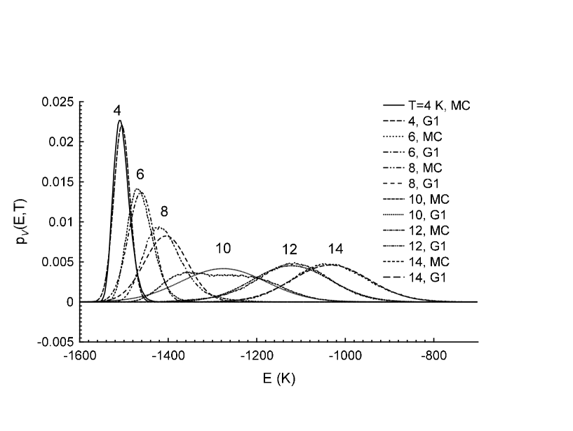
Figure 2: The potential energy pdfs $p_{\mathcal{V}}(E,T)$ for the system of $N=13$ neon particles with atomic mass $m=20.0$ a.u. interacting via Lennard-Jones potential with the parameters $\sigma_{LJ}=2.749$ Å and $\epsilon_{LJ}=35.6$ K as a function of energy $E$ calculated at fixed temperatures $T=4$, 6, 8, 10, 12, and 14 K. The particles are assumed to be in the sphere with the confining radius $R_{c}=2.0\sigma_{LJ}$. MC labels the total results of MC simulations using the asymptotic formula (6) at $\tau=10^{2}$ for $\delta$-function, whereas G1 is the Gaussian approximation Eq. (34) to the MC pdf.

In Fig. 2, the potential energy pdfs $p_{\mathcal{V}}(E,T)$ (labeled by MC) are plotted at fixed temperatures $T=4,6,8,10,12,$ and 14 K. The MC simulations were implemented using the parallel tempering technique, also known as replica exchange Markov chain MC sampling SW:86 ; Gey:91 ; GT:95 ; SO:99 ; ED:05 ; KTH:06 ; SMF:08 ; BNJ:08 ; BJ:11 . In this method several replicas of the same system are simulated in parallel in the canonical ensemble, and usually each replica at a different temperature. In this work, 29 replicas have been run on the even temperature grid, with the temperature step $\Delta T=1$ K, in the interval from 3 to 31 K. Parallel tempering is complementary to any set of MC moves for a system at a single temperature, and such single-system moves are performed between each attempted swap of complete configurations of the systems at adjacent temperatures. The swap moves have been attempted randomly with the probability $P_{swap}=0.1/N$. The high temperature systems are generally able to sample larger volumes of the configuration space, whereas low temperature systems may become trapped in local energy minima. Thus, swapping of configurations ensures that the lower temperature systems can access all contributing regions of the configuration integral, thereby overcoming potential barriers between the local energy minima.

The asymptotic formula (6), with the asymptotic parameter $\tau$ set to 10², has been employed to calculate the $\delta$-function. The energy spectra have been calculated on the equidistant grid of $10^{3}$ points in the range $\left[-2000,1000\right]$ K. The total  number of MC moves has been divided into 50 statistical blocks; the first block data being far from equilibration, have been discarded in further averaging. In each block, the number of MC moves has been $N_{bl}=10^{5}N$. The pdfs in the Gaussian approximation Eq. (34), labeled by G1, are also shown in Fig. 2. Observe that the Gaussian approximation reproduces MC pdfs quite well at higher temperatures $T\geq 12$ K, but there both quantitative and qualitative differences in the shape of distributions are seen at lower temperatures, especially at $T=8$ and 10 K, where the ”melting peak” in heat capacity $C_{V}$ is formed. It should be noticed that although $\delta$-function is a non-negative function (distribution), its asymptotic approximation (6) can in principle be negative at finite values of $\tau$. Thus, although MC pdfs in Fig 2 are seen to be apparently non-negative, we found that in the regions far from the central peaks, where its values are totally corrupted by statistical errors, the MC pdf can take very small negative values $\sim-10^{-6}-10^{-8}$. In these regions negative MC values should be just zeroed. Also, note that usage of a Gaussian representation for the $\delta$-function can be a guarantee for non-negativity of the pdf [suggestion of an anonymous referee].

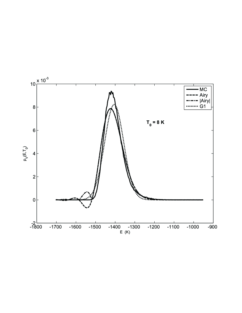
Figure 3: Effect of the 3rd cumulant term on the pdf at $T_{0}=8$ K. Here, ’Airy’ labels the Airy pdf Eq. (37), whereas ’$|\mathrm{Airy}|$’ is the modulus of the Airy pdf. The system and other notations are the same as in Fig. 2.

In Fig. 3, the results of inclusion of the 3rd cumulant term Eq. (37), labeled by Airy, are compared with the G1 and MC pdfs at temperature $T_{0}=8$ K. The corresponding MATLAB function has been used to calculate the Airy function. In general, the effect of the 3rd cumulant on the pdf results in a slight shift of the peak position to lower energies. At $T_{0}=8$ K one can observe small oscillations in the low energy wing of the Airy pdf. Also, the modulus of the Airy curve, labeled by $|\mathrm{Airy}|$, is displayed.

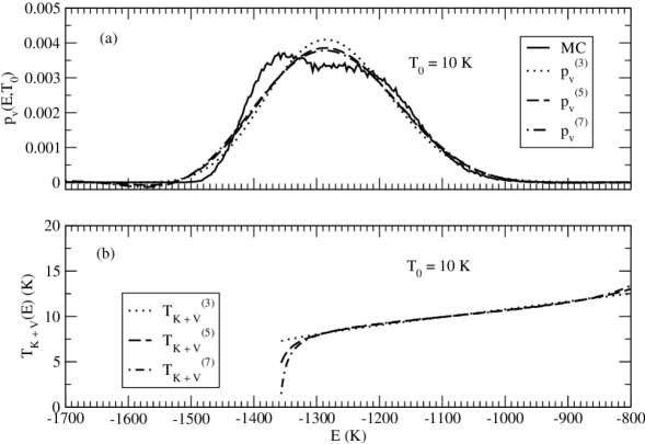
Figure 4: Effects of the higher-order, $k_{max}=3,5$, and 7 cumulants on the pdf (a) and on the statistical temperature (b) at $T_{0}=10$ K. Here, $p_{\mathcal{V}}^{(k_{max)}}$ and $T_{\mathcal{K+V}}^{(k_{max})}$ are the pdfs and the statistical temperatures, respectively, calculated with up to the $k_{max}$-order cumulants included. The MC pdf shows some bimodal structure. The system and other notations are the same as in Fig. 2.

There is a hint that the MC energy distribution in Fig. 2 at $T_{0}=10$ K is bimodal. It is believed that such a bimodal distribution might have a direct connection to the solid-liquid transition in atomic clusters so that a low-energy maximum corresponds to a solid state and a higher one to the liquid state LW:90 ; WB:94 ; SKH:01 . In Fig. 4 (a), the MC pdf at $T_{0}=10$ K is compared to numerical estimates of the integral $p_{\mathcal{V}}^{(k_{max})}$ (27) expressed in terms of the cumulant expansion (32) truncated at $k_{max}=3,5$, and 7. One can see that the numerical results including up to the 7th-order cumulant term are not sufficient to reproduce the hinted bimodal structure in the MC curve. It is expected that inclusion of more cumulant terms will reproduce this structure. Also, numerical results for the statistical temperature using the integral representations (52) are displayed in Fig. 4 (b). The energy dependence of the temperature is seen to be close to a linear one in the neighborhood of $\mu_{c1}=-1273$ K, as qualitatively predicted by Eq. (56). Note that compution of the statistical temperature at the lower energies $E<-1350$ K becomes progressively less accurate because when moving in the low-energy region far from the central peak, where the pdf values get smaller and, thus, relatively less accurate, this ill-defined low-energy region turns out to make a major contribution to the convolution integral (16).

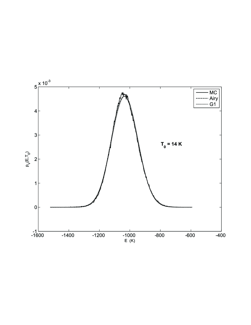
Figure 5: The Airy and the Gaussian pdfs in comparison with the MC pdf at $T_{0}=14$ K. The third cumulant term has a minor effect on the pdf at $T_{0}=14$ K. The system and notations are the same as in Fig. 3.

As temperature increases, the difference between the Airy and G1 pdfs becomes negligible. This is demonstrated in Fig. 5 at $T_{0}=14$ K, where G1 and Airy pdfs are compared with the corresponding MC results.

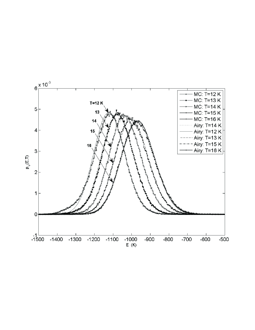
Figure 6: The analytic results from formula (43) applied to the Airy pdf at $T_{0}=14$ and continued to temperatures $T=12,13,15$, and 16 K in comparison with the corresponding MC results. The system and notations are the same as in Fig. 3.

In Fig. 6, we demonstrate how the analytic continuation $T_{0}\rightarrow T$ formula (43) works. With the Airy pdf taken at temperature $T_{0}=14$ K, it is continued to $T=12,13,15$, and 16 K. For comparison, the corresponding MC pdfs are plotted as well. The normalization function $S^{(3)}$ has been evaluated with the help of the analytic formula (45). Obviously, the continuation formula works better when we move to the higher rather than lower temperatures. Moreover, the high-energy wings of the continued pdfs are reproduced better than the low-energy ones. Observe that the low-energy wing of the Airy pdf at $T=12$ K decays faster than the corresponding wing of the MC pdf. The increasing difficulty of analytic continuation to the lower temperatures can be explained by the fact that as one can see the pdfs are shifted to the lower energies as temperature $T$ goes down so that the overlap between the pdfs at different temperatures becomes increasingly smaller. With $T$ decreasing, the difference between inverse temperatures $\Delta\beta>0$ becomes bigger and the exponential factor in (43) grows exponentially. This factor blows up the low-energy wing of the $p(E,T_{0})$ pdf and as a result we observe that the peak maximum of $p(E,T)$ gets a shift to lower energies. Moreover, in the regions far from the center of the $p(E,T_{0})$ pdf, errors are expected to be dominant. As a result, multiplied by an exponentially big factor, these errors either of systematic or statistical nature can generate big deviations from the exact values of $p(E,T)$.

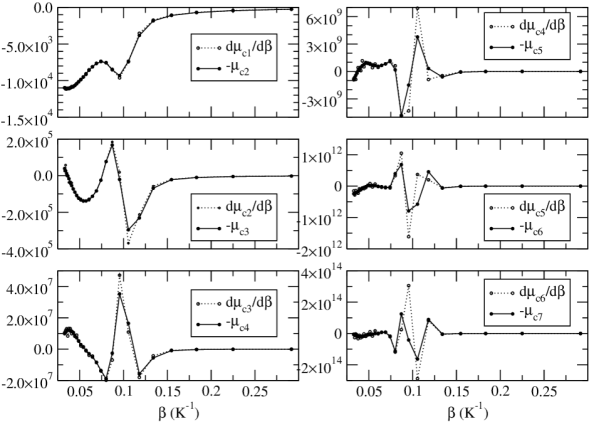
Figure 7: Numerical results illustrating Theorem IV.1, Eq. (21) at $k=1,\ldots,6$. Numerical estimates of the derivatives $d\mu_{ck}/d\beta$ as compared to $-\mu_{c(k+1)}$. The system is the same as in Fig. 2.

Fig. 7 presents numerical results supporting Theorem IV.1. First, we calculated moments up to the 7-th order on the equidistant grid with the step $\Delta T=1$ K in the temperature range from 3 to 31 K. Evaluating higher-order moments is computationally inexpensive since it requires only calculation of extra powers of the potential energy. Then, with the help of Eqs. (94) cumulants $\mu_{ck}$, $k=1,\ldots,7$ can be recursively obtained. The numerical derivatives of cumulants $d\mu_{ck}/d\beta$ are compared with the corresponding higher-order cumulants $\mu_{c(k+1)}$ taken with the minus sign on the inverse temperature $\beta$ scale. In general, agreement is seen to be better for cumulants of lower orders and at higher values of $\beta$. At smaller values of $\beta<0.05$ and in the region $\beta\sim 0.1$ K^-1, where the curves exhibit rapid changes, numerical estimates of the derivatives become more scattered due to errors in the numerical formula for the derivatives, as well as due to statistical errors present in the MC cumulant estimates themselves. Note that when the derivative of $\mu_{ck}$ takes a zero value at some value of $\beta_{ext}$, $\mu_{ck}$ as a function of $\beta$ has an extremum at this point. According to Theorem IV.1, $\mu_{c(k+1)}$ changes the sign at $\beta_{ext}$. Fig. 7 confirms such a behavior.

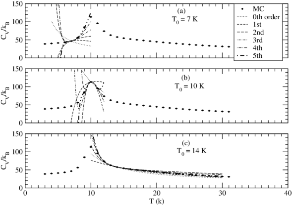
Figure 8: The heat capacity $C_{V}$ in units of the Boltzmann constant $k_{B}$ as a function of temperature $T$. The system is the same as in Fig. 2. The data labeled by MC have been generated with 10${}^{6}N$ MC points in each of 50 statistical blocks, and the error bars are at 95$\%$ confidence level. The analytic continuation of the heat capacity value in the neighborhoods of $T_{0}=7$ (a), 10 (b), and 14 K (c) are done using expansion formula (26). The $k$th-order curves ($k=0,\ldots,5$) are the results of calculation that include maximum up to the $k$th power terms in the expansion (26) in $\Delta\beta$ powers.

In Fig. 8 (a)-(c), making use of the Taylor series expansion (26) we present results of analytic continuation of the heat capacity calculated at temperatures $T_{0}=7$, 10 and 14 K, respectively. For comparison, the results of MC simulation on the equidistant grid of temperatures with the step $\Delta T=1$ K are shown in the range from 3 to 31 K. The data have been generated with 10${}^{6}N$ MC points in each statistical block, and the error bars are at the 95% confidence level. The present MC data coincide within the statistical errors with the results of independent simulations PSD:03b obtained in the temperature range 4 to 14 K. Corresponding to the maximum power of $\Delta\beta$ terms included in expansion (26), the curves including zero, first and so on up to the 5th-order terms are displayed. One can see that dynamics of continuation results is generally improved with inclusion of more terms in the expansion. Thus, we find that the results of the 5th-order curve continuation are good in the intervals $(6,9)$, $(8.5,11),$ and $(11,31)$ K corresponding to $T_{0}=7,\,10$ and 14 K. With increasing temperature $T_{0}$ to 14 K, the interval on which the analytic continuation works is seen to become bigger. In the neighborhood of $T_{0}=10$ K, the heat capacity curve achieves a maximum value. To find this peak position, we solved the polynomial equations (25) for $\Delta\beta$ at $\beta_{0}=0.1$ K^-1 truncated at $k_{\max}=1,2,3,$ and 4. The corresponding roots were obtained using the MATLAB function ’roots’. The results are

$$\begin{array}[]{ccc}\Delta\beta_{peak}^{(k_{\max}=1)}&=&-7.905\cdot 10^{-4}\,\mathrm{K}\\ \Delta\beta_{peak}^{(2)}&=&-7.697\cdot 10^{-4}\,\mathrm{K}\\ \Delta\beta_{peak}^{(3)}&=&-7.726\cdot 10^{-4}\,\mathrm{K}\\ \Delta\beta_{peak}^{(4)}&=&-7.727\cdot 10^{-4}\,\mathrm{K}\end{array}$$

so that the converged peak position temperature is found to be $T_{peak}=10.078$ K. Observe that at $T_{0}=7$ K the slope of the 0th-order curve is negative, while the 1st and higher-order heat capacity curves show positive slopes in qualitative agreement with the behavior of the MC curve.

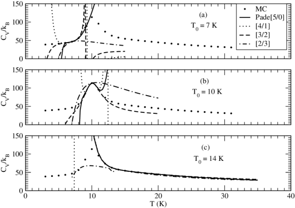
Figure 9: Analytic continuation of the heat capacity by Padé approximants of the orders $[5/0]$, $[4,1]$, $[3,2]$, and $[2,3]$ in the neighborhoods of $T_{0}=7$ (a), 10 (b), and 14 K (c). The system and other labels are the same as in Fig. 8.

The Padé approximants often give better approximation of the function than truncating its Taylor series, and it may still work where the Taylor series does not converge BGM:96 . In Fig. 9 (a)-(c), we compare the MC results with the Padé approximants of various orders $\left[5/0\right],$ $\left[4/1\right],$ $\left[3/2\right]$, and $\left[2/3\right]$ calculated in the neighborhoods of temperatures $T_{0}=7$, 10, and 14 K respectively. Notice that the Padé approximant $\left[5/0\right]$ coincides with the Taylor series truncated at the 5th order. In general, depending on $T_{0}$, the best agreement is seen either for $[5/0]$ or $[3,2]$ Padé approximants. Thus, observe that at $T_{0}=10$ K the Padé approximant $[3/2]$ shows a slightly better behavior than that of $[5/0]$.

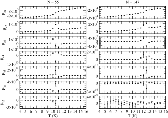
Figure 10: The temperature dependence of cumulants $\mu_{ck}$, $k=1,\ldots,7$, calculated for the system of $N=55$ (left) and 147 (right panel) neon particles. The MC data have been generated with 10${}^{6}N$ and $5\cdot 10^{5}N$ MC points in the left and right panels, respectively, in each of 50 statistical blocks. The error bars are at 95$\%$ confidence level.

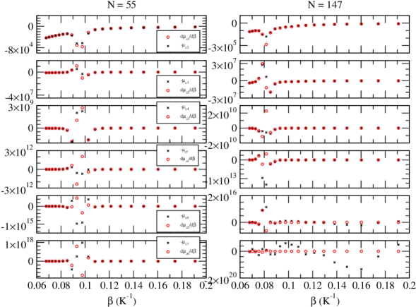
Figure 11: Numerical estimates of the derivatives $d\mu_{ck}/d\beta$, $k=1,\ldots,6$ (red circles) as compared to $-\mu_{c(k+1)}$ (black crosses). The system and statistics are the same as in Fig. 10.

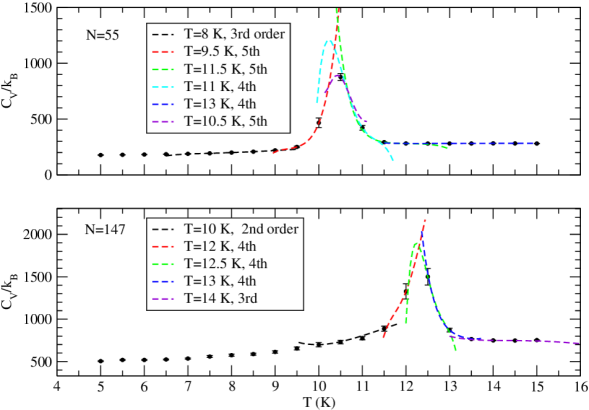
Figure 12: The results of analytic continuation obtained with the help of formula (26) for the system of $N=55$ (upper) and 147 (lower panel) neon particles. Notations are the same as in Fig. 8. Statistics of the MC moves are the same as in Fig. 10.

In Figs. 10-12, the corresponding results for the cumulants, their derivatives and the heat capacity curves are displayed for $N=55$ and 147 neon particles. The confining radius is set to be $R_{c}=0.85\sigma_{LJ}N^{1/3}$. Notice that the MC data have been generated with $N_{bl}=10^{6}N$ MC moves for the system of $N=55$ particles and with $N_{bl}=5\cdot 10^{5}N$ MC points for $N=147$ particles in each of 50 statistical blocks. The size of the error bars obtained for the cumulants in Fig. 10 tends to become bigger for the cumulants of higher orders, but decrease when temperature goes up, except for the region where the heat capacity reveals a peak. In Fig. 11, the derivatives $d\mu_{ck}/d\beta$, $k=1,\ldots,6$ are compared to the corresponding cumulants $-\mu_{c(k+1)}$. The agreement is quite good, additionally supporting Theorem IV.1. Deviations between $d\mu_{ck}/d\beta$ and $-\mu_{c(k+1)}$ are most pronounced in the regions of cumulant’s rapid change and these deviations are caused either by the statistical or systematic errors in numerical estimates of the derivatives and the corresponding cumulants. Thus, one can see that the 7th-order cumulant for $N=147$ particles, shown in the right panel of Fig. 10, is poorly converged at current value of $N_{bl}$ since it is almost totally in error at $T\leq 12$ K. As expected, this results in a poor agreement observed in the right panel of Fig. 11 between the derivative $d\mu_{c6}/d\beta$ and the cumulant $-\mu_{c7}$. Fig. 12 demonstrates the results of analytic continuation obtained for the heat capacity $C_{V}$ using formula (26). From analytic continuation curves we get the following estimates for the peak positions $T_{peak}=10.44$ and $12.25$ K for the system of $N=55$ and 147 particles, respectively.

Finally, let us consider the convergence issue, that is, how errors present in the MC estimates may affect the results of continuation. The MC estimates for cumulants can be represented as $\mu_{ck}=\mu_{ck}^{exact}+\varepsilon_{ck}$, where $\mu_{ck}^{exact}$ is an exact value of the $k$th-order cumulant and $\varepsilon_{ck}$ is an error in its estimate. We assume that cumulant estimates have been generated at a fixed number of MC moves. The longer MC moves are generated the less errors one gets in $\mu_{ck}$’s. Notice that we cannot directly compare the sizes of errors in cumulants of different orders since they have different physical dimensions: $[\mu_{ck}]=[{\rm Energy}]^{k}$. In the continuation formula (26), the $k$th-order cumulant enters multiplied by the $k$th power of a small expansion parameter $\Delta\beta$, so that the continued 2nd-order cumulant can be written as

$$\mu_{c2}(\beta) = \mu_{c2}^{exact}(\beta)+\varepsilon_{c2}^{tot}(\beta),$$

$$\mu_{c2}^{exact}(\beta) = \mu_{c2}^{exact}(\beta_{0})-\dfrac{\mu_{c3}^{exact}(\beta_{0})}{1!}\Delta\beta+\dfrac{\mu_{c4}^{exact}(\beta_{0})}{2!}(\Delta\beta)^{2}+\cdots,$$

$$\varepsilon_{c2}^{tot}(\beta) = \varepsilon_{c2}(\beta_{0})-\dfrac{\varepsilon_{c3}(\beta_{0})}{1!}\Delta\beta+\dfrac{\varepsilon_{c4}(\beta_{0})}{2!}(\Delta\beta)^{2}+\cdots$$ (84)

One can see that the total error $\varepsilon_{c2}^{tot}(\beta)$ in the continued 2nd-order cumulant is defined by the sum of errors in the 2nd- and higher-order cumulants at $\beta_{0}$, contributions from the higher-order cumulant’s errors are being multiplied by the powers of the expansion parameter $\Delta\beta$. With the growth of $\Delta\beta$, the contribution of the 3rd- and higher-order cumulant’s errors to $\varepsilon_{c2}^{tot}(\beta)$ increases and at some value, which we call a radius of convergence $\Delta\beta_{conv}$, its contribution becomes comparable to the size of the 2nd-order cumulant’s error $\varepsilon_{c2}(\beta_{0})$. We do not know exactly errors in cumulants (errors are random numbers) but their size can be estimated by 2$\sigma_{ck}$’s, by the two standard deviations in a usual way (by error bars in Fig. 10). Thus, one can estimate the raduis of convergence $\Delta\beta_{conv}^{(k\to 2)}$ for the $k$th-order cumulant ($k>2$) by the expression

$$|\Delta\beta_{conv}^{(k\to 2)}|=\left((k-2)!\dfrac{\sigma_{c2}}{\sigma_{ck}}\right)^{1/(k-2)}$$ (85)

Using the relationship between inverse and direct temperature scales $\Delta\beta=\beta-\beta_{0}=1/T-1/T_{0}\approx-\Delta T/T_{0}^{2}$, where $\Delta T=T-T_{0}$, one finds the corresponding radius of convergence in the temperature scale

$$\Delta T_{conv}^{(k\to 2)}=T_{0}^{2}\left((k-2)!\dfrac{\sigma_{c2}}{\sigma_{ck}}\right)^{1/(k-2)}$$ (86)

It roughly defines the temperature range within which the errors present in the $k$th-order cumulant will produce the same order errors as in the $\mu_{c2}(\beta_{0})$.

The $2\sigma_{ck}$’s obtained for the cluster of $N=55$ neon particles at low $T_{0}=5$ and 15 K and high temperatures $T_{0}=100$ and 300 K are summarized in Table 1. Observe how the magnitude of errors in cumulants increases, roughly by an order, as the number of MC moves specified by the parameter $f_{MC}$ decreases by two orders at $T_{0}=100$ K.

Table 1: The two standard deviations $2\sigma_{ck}$ ($k=2,\ldots,7$) calculated for the $k$th-order cumulant at low $T_{0}=5$, 15 (the size of error bars in Fig. 10) and at high temperatures $T_{0}=100$ and 300 K using 50 statistical blocks. The number of Monte Carlo moves in a single statistical block is $N_{MC}=f_{MC}N$, where $N=55$ is the number of neon particles in the LJ cluster.

$T_{0}$ (K)	$f_{MC}$	$2\sigma_{c2}$ (K2)	$2\sigma_{c3}$ (K3)	$2\sigma_{c4}$ (K4)	$2\sigma_{c5}$ (K5)	$2\sigma_{c6}$ (K6)	$2\sigma_{c7}$ (K7)
5	106	$3.0\cdot 10^{0}$	$2.5\cdot 10^{2}$	$2.2\cdot 10^{4}$	$1.2\cdot 10^{8}$	$2.2\cdot 10^{12}$	$4.2\cdot 10^{16}$
15	106	$1.6\cdot 10^{2}$	$4.6\cdot 10^{4}$	$1.9\cdot 10^{7}$	$7.7\cdot 10^{9}$	$4.8\cdot 10^{12}$	$7.0\cdot 10^{15}$
100	106	$1.0\cdot 10^{2}$	$4.0\cdot 10^{4}$	$3.5\cdot 10^{7}$	$3.2\cdot 10^{10}$	$3.2\cdot 10^{13}$	$5.0\cdot 10^{16}$
100	105	$2.5\cdot 10^{2}$	$1.6\cdot 10^{5}$	$1.1\cdot 10^{8}$	$1.2\cdot 10^{11}$	$1.8\cdot 10^{14}$	$3.7\cdot 10^{17}$
100	104	$6.7\cdot 10^{2}$	$4.7\cdot 10^{5}$	$2.9\cdot 10^{8}$	$2.5\cdot 10^{11}$	$2.3\cdot 10^{14}$	$2.1\cdot 10^{17}$
300	106	$3.9\cdot 10^{2}$	$6.5\cdot 10^{5}$	$1.7\cdot 10^{9}$	$5.2\cdot 10^{12}$	$2.1\cdot 10^{16}$	$1.1\cdot 10^{20}$

Table 2: The radius of convergence for the $k$th-order cumulant $\Delta T_{conv}^{(k\to 2)}$ calculated with the help of Eq. (86) and the data from Table 1. Other notations are the same as in Table 1.

$T_{0}$ (K)	$f_{MC}$	$\Delta T_{conv}^{(3\to 2)}$ (K)	$\Delta T_{conv}^{(4\to 2)}$ (K)	$\Delta T_{conv}^{(5\to 2)}$ (K)	$\Delta T_{conv}^{(6\to 2)}$ (K)	$\Delta T_{conv}^{(7\to 2)}$ (K)
5	106	0.3	0.4	0.6	0.06	0.04
15	106	0.8	0.9	1.1	1.2	1.2
100	106	25	24	26	29	30
100	105	16	21	23	24	24
100	104	14	21	25	29	33
300	106	54	61	69	74	76

Making use of the data in Table 1, we can estimate radii of convergence for the higher-order (3-7) cumulants with the help of Eq. (86); the results of evaluation are summarized in Table 2. Observe that at $T_{0}=5$ K, the higher-order, 6th and 7th-order, cumulants appear to be non-converged since their radii of convergence are by an order of magnitude smaller than the values obtained for the 3rd-, 4th-, and 5th-order cumulants. At higher temperatures shown in Table 2, all the cumulants seem to be well converged; the smallest radius of convergence is generally found for the 3rd-order cumulant’s contribution. As an empirical rule, we find that the radius of convergence is roughly proportional to the temperature $T_{0}$. Notice that at $T_{0}=100$ K, when the number of MC moves drops down by two orders, the radius of convergence $\Delta T_{conv}^{(3\to 2)}$ is reduced by about two times only.

X Concluding remarks

In obtaining reliable estimates of thermal averages in realistic, multidimensional, classical or quantum many- or few-body systems, the MC simulation is often the only way of getting right answers. The simulated averages depend on thermodynamic parameters, such as temperature, volume etc., and/or interaction parameters between the particles. Therefore, in order to avoid many time-consuming runs of the MC codes at various parameters, it is important to develop robust analytic techniques that allow us to continue the MC data in the neighborhood of a set of prescribed parameter values. The key finding of this work is a simple relationship Eq. (21) between derivatives and the higher-order cumulants. Since many important thermodynamic quantities, such as energy and heat capacity, can be expressed in terms of cumulants, this theorem provides an analytic tool or bridge to continue MC data in the neighborhood of a control parameter value, say, $\beta_{0}$ or to fill a gap by constructing an analytic bridge in between of two neighboring parameters $\beta_{0}$ and $\beta_{1}$.

To find an optimal numerical scheme to evaluate the cumulants up to the $k_{max}$th-order (in our examples $k_{max}=7$), it is important to estimate the amount of numerical work required. A reasonable estimate of this time is the number of potential function calls $N_{call}$ required to compute a thermodynamic quantity, e.g., the heat capacity. In a single MC move, the system moves to a new position and one has to calculate the potential function $V_{i}=V(X_{i})$ one time at a new position $X_{i}$ so that $N_{call}=N_{bl}$ where $N_{bl}$ is a total number of MC moves in a single statistical block. To calculate cumulants up to the $k_{max}$th-order, one has to compute additionally $k_{max}-1$ powers $V_{i}^{k}$, $k=2,\ldots,k_{max}$ or perform $k_{max}-1$ multiplications of the known potential function value $V_{i}$. These multiplications are computationally cheap and do not depend on the size of the system. Therefore, as estimated the amount of numerical work to evaluate the higher-order cumulants will be practically the same as in the standard parallel tempering scheme which requires evaluation of only $V_{i}$ and $V_{i}^{2}$ values.

By Eqs. (27)-(31), the energy pdfs can also be expressed in terms of cumulants. Truncating the cumulant expansion at $k_{max}$, we have derived analytic expressions (33), (34), and (37) for the pdfs at $k_{max}=1,2,$ and 3 respectively. The higher-order energy pdfs truncated at $k_{max}\geq 4$ can be obtained either by evaluating the $\tau$-integral numerically or by applying an appropriate (saddle-point) asymptotic method.

Generalizations to a multi-parameter classic system are rather straightforward and can be expressed by the Theorem VII.1. Using this theorem, one can easily develop similar analytic continuation formulas, such as Eqs. (68), in terms of the higher-order multi-variate cumulants in the multi-parametric space. The path integral Feynman-Kac representation of the density matrix is a very useful formulation of the quantum statistical equilibrium operator since it basically reduces the problem of analytic continuation in quantum case to the corresponding problem in multi-parametric classical systems. Of course, technically this reduction can be done if the original infinite-dimensional integration over the path variables can be replaced somehow by a finite-dimensional one. We considered several possible scenarios, having different convergence properties with respect to the number of path variables, of such infinite-to-finite dimensional integral replacements in Section VIII.

Numerical testing of Theorem IV.1, analytic continuation formulas for the energy pdfs and heat capacity curves has been exemplified by an LJ classical cluster sytem in Section IX. By now, usefulness of analytic continuation formulas in multi-parametric classical and quantum systems have not yet been tested numerically. Further numerical investigations of interesting multi-parameter systems are of special interest. The results of such investigations when available will be published elsewhere.

Appendix A Moments versus Cumulants

Relationships between univariate cumulants and moments can be derived from the moment-generating function Ku:62

$$M(t) = \left\langle\exp\left(tH\right)\right\rangle=1+\sum_{k=1}^{\infty}\dfrac{t^{k}}{k!}\mu_{k}$$ (87)

$$= \exp\left[\sum_{k=1}\dfrac{t^{k}}{k!}\mu_{ck}\right]$$

where $\mu_{k}\equiv\left\langle H^{k}\right\rangle$ are called moments. Assuming the average of 1 to be nonzero, we conclude that $\ln\left\langle\exp\left(tH\right)\right\rangle$ is an analytic function of $t$, in a vicinity of zero. Therefore, it has a Taylor expansion with respect to $t$. This expansion is called cumulant expansion; the coefficients $\mu_{ck}$ of the expansion are called cumulants. Thus, cumulants in terms of moments are expressible by the formula

$$\mu_{ck}=\sum_{r=1}^{k}\dfrac{(-1)^{r+1}}{r}\sum_{p_{1},\ldots,p_{r}\in C_{kr}}\dfrac{k!}{p_{1}!\cdots p_{r}!}\mu_{p_{1}}\cdots\mu_{p_{r}}$$ (88)

where the summation of the integer indices $p_{1},\cdots,p_{r}\geq 1$ is restricted by the relation

$$C_{kr}=\left\{(p_{1},\cdots,p_{r}):\;\sum_{j=1}^{r}p_{j}=k\right\}$$

In order to calculate the $k$-th order cumulant one needs moments up to the $k$-th order.

On the other hand, moments can be expressed via cumulants by a similar formula

$$\mu_{k}=\sum_{r=1}^{k}\dfrac{1}{r!}\sum_{\begin{subarray}{c}p_{1},\ldots,p_{r}\in C_{kr}\end{subarray}}\dfrac{k!}{p_{1}!\cdots p_{r}!}\mu_{cp_{1}}\cdots\mu_{cp_{r}}$$ (89)

The $k$th moment $\mu_{k}$ is a $k$th-degree polynomial in the first $k$ cumulants. These polynomials have a remarkable combinatorial interpretation: the coefficients count certain partitions of sets. A general form of these polynomials is

$$\mu_{k}=\sum_{\pi}\prod_{S\in\pi}\mu_{c|S|}$$ (90)

where $\pi$ runs through the list of all partitions of a set of size $k$; ”$S\in\pi$” means $S$ is one of the ”blocks” into which the set is partitioned; and $|S|$ is the size of the set $S$. To better understand how Eq. (90) corresponds to (89) let us consider all possible partitions of the set of natural numbers $\{1,2,\ldots,k\}$. We can divide all possible partitions $\{\pi\}$ into disjoint groups $\{\pi\}=\{\pi_{1},\ldots,\pi_{k}\}$ such that the number of blocks in a particular partition $\pi_{r}$, $r=1,\ldots,k$ is equal to $r$. For example, in case of $k=3$ we obtain the set of all possible partitions classified as $\{\pi_{1},\pi_{2},\pi_{3}\}$. Here, $\pi_{1}$ includes an ”improper” partition $(123)$. The size of the $(123)$ partition is three. $\pi_{2}$ corresponds to partitions into two blocks: $(12)3$, $(13)2$, $(23)1$, with sizes of blocks being two and one. $\pi_{3}$ splits the set into three blocks $(1)(2)(3)$, each block of size one. Round parenthesis show how the set is partitioned. The total number of partitions of a $k$-element set is the Bell number $B_{k}$: $B_{0}=1$, $B_{1}=1$, $B_{2}=2$, $B_{3}=5$. Bell numbers satisfy the recursion $B_{k+1}=\sum_{n=0}^{k}\binom{k}{n}B_{n}$, where $\binom{k}{n}$ is the binomial coefficient.

If $S_{1},\ldots,S_{r}\in\pi_{r}$ are $r$ blocks into which the set can be divided, then Eq. (90) can be rewritten as

$$\mu_{k}=\sum_{r=1}^{k}\sum_{S_{1},\ldots,S_{r}\in\pi_{r}}\mu_{c|S_{1}|}\cdots\mu_{c|S_{r}|}$$ (91)

where inner summation runs over all possible non-empty, disjoint blocks. Then, each $r$-term in Eq. (89) corresponds to the $r$-term in (91):

$$\dfrac{1}{r!}\sum_{\begin{subarray}{c}p_{1},\ldots,p_{r}\in C_{kr}\end{subarray}}\dfrac{k!}{p_{1}!\cdots p_{r}!}\mu_{cp_{1}}\cdots\mu_{cp_{r}}=\sum_{S_{1},\ldots,S_{r}\in\pi_{r}}\mu_{c|S_{1}|}\cdots\mu_{c|S_{r}|}$$ (92)

Indeed, the multinomial coefficient

$$\left(\begin{array}[]{ccc}&k&\\ p_{1}&\cdots&p_{r}\end{array}\right)=\dfrac{k!}{p_{1}!\cdots p_{r}!}$$ (93)

in the left-hand-side is the number of ways of grouping $k$ objects (numbers) into $r$ groups (blocks) of sizes $p_{1},\ldots,p_{r}$, when the order within each group does not matter. The summation over blocks in the right-hand side can be carried out into two steps. First, the summation over all possible block’s sizes $|S_{1}|=p_{1},\ldots,|S_{r}|=p_{r}$ such that $p_{1}\leq\cdots\leq p_{r}$ and then summing up over blocks at fixed sizes of blocks

$$\sum_{S_{1},\ldots,S_{r}\in\pi_{r}}\ldots=\sum_{\begin{subarray}{c}p_{1}\leq\cdots\leq p_{r}\\ p_{1}+\cdots+p_{r}=k\end{subarray}}\sum_{|S_{1}|=p_{1},\ldots,|S_{r}|=p_{r}}\ldots$$

Obviously, the inner summation will result in the same multinomial coefficient (93) as in the left-hand side of (92). Finally, notice that the summed function $\mu_{cp_{1}}\cdots\mu_{cp_{r}}$ and the multinomial coefficient are totally symmetric functions with respect to permutations of $p_{1},\ldots,p_{r}$ indexes and $r!$ is the number of their permutations. This symmetry results in

$$\dfrac{1}{r!}\sum_{\begin{subarray}{c}p_{1},\cdots,p_{r}\\ p_{1}+\cdots+p_{r}=k\end{subarray}}\ldots=\sum_{\begin{subarray}{c}p_{1}\leq\cdots\leq p_{r}\\ p_{1}+\cdots+p_{r}=k\end{subarray}}\ldots$$

This proves Eq. (92).

Using Eq. (89) or (91), one obtains the following expressions for the first seven moments in terms of cumulants

$$\mu_{1} = \mu_{c1},$$

$$\mu_{2} = \mu_{c2}+\mu_{c1}^{2},$$

$$\mu_{3} = \mu_{c3}+3\mu_{c2}\mu_{c1}+\mu_{c1}^{3},$$

$$\mu_{4} = \mu_{c4}+4\mu_{c3}\mu_{c1}+3\mu_{c2}^{2}+6\mu_{c2}\mu_{c1}^{2}+\mu_{c1}^{4},$$

$$\mu_{5} = \mu_{c5}+5\mu_{c4}\mu_{c1}+10\mu_{c2}\mu_{c3}+10\mu_{c3}\mu_{c1}^{2}+15\mu_{c2}^{2}\mu_{c1}+10\mu_{c2}\mu_{c1}^{3}+\mu_{c1}^{5},$$

$$\mu_{6} = \mu_{c6}+6\mu_{c5}\mu_{c1}+15\mu_{c2}\mu_{c4}+10\mu_{c3}^{2}+15\mu_{c4}\mu_{c1}^{2}$$

$$+ 60\mu_{c3}\mu_{c2}\mu_{c1}+15\mu_{c2}^{3}+20\mu_{c3}\mu_{c1}^{3}+45\mu_{c2}^{2}\mu_{c1}^{2}+\mu_{c1}^{6},$$

$$\mu_{7} = \mu_{c7}+7\mu_{c6}\mu_{c1}+21\mu_{c2}\mu_{c5}+35\mu_{c3}\mu_{c4}+21\mu_{c5}\mu_{c1}^{2}$$ (94)

$$+ 105\mu_{c4}\mu_{c2}\mu_{c1}+70\mu_{c3}^{2}\mu_{c1}+105\mu_{c3}\mu_{c2}^{2}+35\mu_{c4}^{2}\mu_{c1}^{3}$$

$$+ 210\mu_{c2}\mu_{c3}\mu_{c1}^{2}+105\mu_{c2}^{3}\mu_{c1}+35\mu_{c3}\mu_{c1}^{4}+105\mu_{c2}^{2}\mu_{c1}^{3}+21\mu_{c2}\mu_{c1}^{5}+\mu_{c1}^{7}$$

These equations relating the cumulants and the moments can also be interpreted as recurrence relations that allow the expression of the higher-order cumulants in terms of lower-order ones.

Appendix B Proof of Eq. (21)

The proof is by induction. At $k=1$, the statement of theorem follows directly from Eq. (20) and definitions of the first two cumulants $\mu_{c1}=\mu_{1}$ and $\mu_{c2}=\mu_{2}-\mu_{1}^{2}$. Let us assume that Eq. (21) is valid at $k=1,\ldots,p$; we have to prove its validity at $k=p+1$. Making use of combinatorial representation (91), the $(p+1)$-st moment can be written as KFD:10

$$\mu_{p+1}=\sum\limits_{r=1}^{p+1}\sum\limits_{S_{1},\ldots,S_{r}}\mu_{c|S_{1}|}\ldots\mu_{c|S_{r}|}$$ (95)

where $S_{1},\ldots,S_{r}$ denote a partition of a set of natural numbers $\left\{1,\ldots,p+1\right\}$. If blocks $S_{1},\ldots,S_{r}$ contain, respectively, $k_{1},\ldots,k_{r}$ elements [numbers] such that $k_{1}+\ldots+k_{r}=p+1$, then $\mu_{c|S_{1}|}=\mu_{ck_{1}},\ldots,\mu_{c|S_{r}|}=\mu_{ck_{r}}$. The term in (95) for $r=1$ corresponds to $\mu_{c(p+1)}$, so that Eq. (95) can be rewritten as

$$\mu_{c(p+1)}=\mu_{p+1}-\sum\limits_{r=2}^{p+1}\sum\limits_{S_{1},\ldots,S_{r}}\mu_{c|S_{1}|}\ldots\mu_{c|S_{r}|}$$ (96)

where the summation is performed over the ”proper partitions” when $r\geq 2$. Observe that the sizes $k_{1},\ldots,k_{r}$ of ”proper partitions” in (96) cannot be bigger than $p$. Differentiating (96) with respect to $\beta$, we get

$$\dfrac{d\mu_{c(p+1)}}{d\beta} = -\mu_{p+2}+\mu_{p+1}\mu_{1}$$ (97)

$$- \sum\limits_{r=2}^{p+1}\sum\limits_{S_{1},\ldots,S_{r}}\dfrac{\mu_{c|S_{1}|}}{d\beta}\ldots\mu_{c|S_{r}|}-\cdots$$

$$- \sum\limits_{r=2}^{p+1}\sum\limits_{S_{1},\ldots,S_{r}}\mu_{c|S_{1}|}\ldots\dfrac{\mu_{c|S_{r}|}}{d\beta}$$

where in the first line we have used Eq. (20) at $k=p+1$. The term $\mu_{p+1}\mu_{1}$ can be rewritten as

$$\mu_{p+1}\mu_{1}=\sum\limits_{r=1}^{p+1}\sum\limits_{S_{1},\ldots,S_{r}}\mu_{c|S_{1}|}\ldots\mu_{c|S_{r}|}\mu_{c|T|}$$ (98)

Here, to the set of natural numbers $\{1,\ldots,p+1\}$ we added the number $p+2$ so that in the partition $S_{1},\ldots,S_{r},T$ the $S$’s correspond to all possible blocks partitioning the set $\{1,\ldots,p+1\}$ and $T$ is related to a fixed element, the number $p+2$. Evidently, $|T|=1$ and $\mu_{c|T|}=\mu_{c1}=\mu_{1}$. Further, by induction conjecture one can use Eq. (21) for the cumulant derivatives in the second and next lines

$$\dfrac{\mu_{c|S_{1}|}}{d\beta} = -\mu_{c(k_{1}+1)}=-\mu_{c|S_{1}\cup T|},$$

$$\vdots$$

$$\dfrac{\mu_{c}\left[S_{r}\right]}{d\beta} = -\mu_{c(k_{r}+1)}=-\mu_{c|S_{r}\cup T|},$$ (99)

where $S_{1}\cup T,\ldots,S_{r}\cup T$ denote that to a particular partition of $\{1,\ldots,p+1\}$ we add consecutively a fixed element $T=p+2$ to $S_{1},\ldots,S_{r}$ blocks. Substituting Eqs. (98) and (99) into (97), we get

$$\dfrac{d\mu_{c(p+1)}}{d\beta} = -\mu_{p+2}+\sum\limits_{r=1}^{p+1}\sum\limits_{S_{1},\ldots,S_{r}}\mu_{c|S_{1}|}\ldots\mu_{c|S_{r}|}\mu_{c|T|}$$ (100)

$$+ \sum\limits_{r=2}^{p+1}\sum\limits_{S_{1},\ldots,S_{r}}\mu_{c|S_{1}\cup T|}\ldots\mu_{c|S_{r}|}+\cdots$$

$$+ \sum\limits_{r=2}^{p+1}\sum\limits_{S_{1},\ldots,S_{r}}\mu_{c|S_{1}|}\ldots\mu_{c|S_{r}\cup T|}$$

Evidently, summing over $S_{1},\ldots,S_{r}$ partitions of $\{1,\ldots,p+1\}$ with inclusion of a fixed element $T$ is equivalent to

$$\sum\limits_{r=2}^{p+2}\sum\limits_{S_{1},\ldots,S_{r}}$$

where $S_{1},\ldots,S_{r}$ is a partition of $\{1,\ldots,p+2\}$ at $r\geq 2$, so that Eq. (100) can be rewritten as

$$\dfrac{d\mu_{c(p+1)}}{d\beta} = -\mu_{p+2}+\sum\limits_{r=2}^{p+2}\sum\limits_{S_{1},\ldots,S_{r}}\mu_{c|S_{1}|}\ldots\mu_{c|S_{r}|}$$ (101)

$$= -\mu_{c(p+2)}$$

Here, in transition to the second line, we employed Eq. (96), where a substitution $p\rightarrow p+1$ has been made. This completes the proof.

Appendix C Multivariate Cumulants and Proof of Theorem VII.1

Similar to Eq. (87), multivariate moments and cumulants are defined via the moment generating function Ku:62

$$M(t_{1},\ldots,t_{p}) = \left\langle\exp\left(\sum_{k=1}^{p}t_{k}H_{k}\right)\right\rangle=1+\sum_{k_{1},\ldots,k_{p}}\dfrac{t_{1}^{k_{1}}\cdots t_{p}^{k_{p}}}{k_{1}!\cdots k_{p}!}\mu_{k_{1},\ldots,k_{p}}$$ (102)

$$= \exp\left[\sum_{k_{1},\ldots,k_{p}}\dfrac{t_{1}^{k_{1}}\cdots t_{p}^{k_{p}}}{k_{1}!\cdots k_{p}!}\mu_{ck_{1},\ldots,k_{p}}\right]$$

where $\mu_{k_{1},\ldots,k_{p}}\equiv\left\langle H_{1}^{k_{1}}\cdots H_{p}^{k_{p}}\right\rangle$ and summation runs over non-negative integers $k_{1},\ldots,k_{p}$ except for $k_{1}=\ldots=k_{p}=0$. Using Eq. (102), one can derive explicit relations between $p$-dimensional moments and cumulants, multivariate generalizations of Eqs. (87) and (89); see Appendix in Mee:57 . Following Mee:57 , it is convenient to introduce compact notations for multi-indexes $\mathbf{k}=(k_{1},\ldots,k_{p})$, as well as for the product of powers of multivariate variables $\mathbf{t}^{\mathbf{k}}=t_{1}^{k_{1}}\cdots t_{p}^{k_{p}}$, and product of factorials $\mathbf{k}!=k_{1}!\cdots k_{p}!$. In these notations, Eq. (102) reads

$$\sum_{\mathbf{k}}\frac{\mathbf{t}^{\mathbf{k}}}{\mathbf{k}!}\mu_{\mathbf{k}} = \exp\left[\sum_{\mathbf{k}}\frac{\mathbf{t}^{\mathbf{k}}}{\mathbf{k}!}\mu_{c\mathbf{k}}\right]-1$$ (103)

$$= \sum_{r=1}^{\infty}\frac{1}{r!}\sum_{\mathbf{n}_{1}\neq\mathbf{0},\ldots,\mathbf{n}_{r}\neq\mathbf{0}}\frac{\mathbf{t}^{\mathbf{n}_{1}+\ldots+\mathbf{n}_{r}}}{\mathbf{n}_{1}!\cdots\mathbf{n}_{r}!}\mu_{c\mathbf{n}_{1}}\cdots\mu_{c\mathbf{n}_{r}}$$

In the second line, the exponential function has been expanded in Taylor’s series and multi-indexes in the inner-sum are non-negative such that $\mathbf{n}_{1}\neq\mathbf{0},\ldots,\mathbf{n}_{r}\neq\mathbf{0}$. Differentiation of Eq. (103) by applying the multi-index differential operator

$$D_{\mathbf{t}}^{\mathbf{k}}=\frac{\partial^{|\mathbf{k}|}}{\partial t_{1}^{k_{1}}\cdots\partial t_{p}^{k_{p}}}$$ (104)

to the both sides and then putting $\mathbf{t}=\mathbf{0}$ yields a multivariate analogue of (89)

$$\mu_{\mathbf{k}}=\sum_{r=1}^{|\mathbf{k}|}\frac{1}{r!}\sum_{\begin{subarray}{c}\mathbf{n}_{1}\neq\mathbf{0},\ldots,\mathbf{n}_{r}\neq\mathbf{0}\\ \mathbf{n}_{1}+\ldots+\mathbf{n}_{r}=\mathbf{k}\end{subarray}}\frac{\mathbf{k}!}{\mathbf{n}_{1}!\cdots\mathbf{n}_{r}!}\mu_{c\mathbf{n}_{1}}\cdots\mu_{c\mathbf{n}_{r}}$$ (105)

where $|\mathbf{k}|=k_{1}+\ldots+k_{p}$.

In multi-dimensional case, Eq. (91) remains valid if the single index $k$ is replaced by a multi-dimensional one $\mathbf{k}$, and partitioning $\pi_{r}$ of the set $\{1,2,\ldots,k\}$ is replaced by partitioning of the ordered set of multi-indexes $(\{1,\ldots,k_{1}\};\{1,\ldots,k_{2}\};\ldots;\{1,\ldots,k_{p}\})$:

$$\mu_{\mathbf{k}} = \sum_{r=1}^{|\mathbf{k}|}\sum_{S_{1},\ldots,S_{r}\in\pi_{r}}\mu_{c|S_{1}|}\cdots\mu_{c|S_{r}|}$$ (106)

$$= \sum_{r=1}^{|\mathbf{k}|}\sum_{\begin{subarray}{c}\mathbf{n}_{1}\leq\cdots\leq\mathbf{n}_{r}\\ \mathbf{n}_{1}+\cdots+\mathbf{n}_{r}=\mathbf{k}\end{subarray}}\sum_{|S_{1}|=\mathbf{n}_{1},\ldots,|S_{r}|=\mathbf{n}_{r}}\mu_{c\mathbf{n}_{1}}\cdots\mu_{c\mathbf{n}_{r}}$$

where $S_{1},\ldots,S_{r}$ are all possible blocks into which the set of multi-indexes can be divided. The summation over blocks in the second line is organized as follows. The first summation over $r$ defines the number of blocks $S_{1},\ldots,S_{r}$ partitioning the set of multi-indexes. The second summation runs over all possible sizes of blocks such that $\mathbf{n}_{1}+\cdots+\mathbf{n}_{r}=\mathbf{k}$. In components, if $\mathbf{n}_{i}=(n_{i1},n_{i2},\ldots,n_{ip})$, $i=1,\ldots,r$ [the first subindex labels the block’s number, the second one is due to variable’s number], we have constraining equations

$$\mathbf{n}_{1}+\cdots+\mathbf{n}_{r}=\mathbf{k}\quad\Leftrightarrow\quad\begin{cases}n_{11}+\cdots+n_{r1}=k_{1}\\ n_{12}+\cdots+n_{r2}=k_{2}\\ {1}\\ n_{1p}+\cdots+n_{rp}=k_{p}\end{cases}$$ (107)

and inequalities specifying the partial ordering conditions

$$\mathbf{n}_{1}\leq\cdots\leq\mathbf{n}_{r}\quad\Leftrightarrow\quad\begin{cases}n_{11}\leq n_{21}\leq\cdots\leq n_{r1}\\ n_{12}\leq n_{22}\leq\cdots\leq n_{r2}\\ {1}\\ n_{1p}\leq n_{2p}\leq\cdots\leq n_{rp}\end{cases}$$ (108)

The inner summation over all possible blocks at fixed sizes results in

$$\sum_{|S_{1}|=\mathbf{n}_{1},\ldots,|S_{r}|=\mathbf{n}_{r}}\mu_{c\mathbf{n}_{1}}\cdots\mu_{c\mathbf{n}_{r}}=\dfrac{\mathbf{k}!}{\mathbf{n}_{1}!\cdots\mathbf{n}_{r}!}\mu_{c\mathbf{n}_{1}}\cdots\mu_{c\mathbf{n}_{r}}$$ (109)

where

$$\dfrac{\mathbf{k}!}{\mathbf{n}_{1}!\cdots\mathbf{n}_{r}!}=\dfrac{k_{1}!\cdots k_{p}!}{n_{11}!\cdots n_{1p}!\cdots n_{r1}!\cdots n_{rp}!}$$ (110)

Observe that the multi-index-multinomial coefficient (110) in the right-hand side of (109) is the same as in (105). As in Appendix A, due to symmetry of the summed functions with respect to permutations of multi-indexes $\mathbf{n}_{1},\ldots,\mathbf{n}_{r}$, we obtain that Eqs. (105) and (106) are equivalent representations for multivariate moments. The latter representation is helpful in proving the multivariate analogue of the theorem on cumulant’s derivative.

The proof of Theorem VII.1 is by induction and quite similar to the proof of Theorem IV.1 done in previous Appendix. The only complication is due to multi-index nomenclature.

Figure 1: A closed rectangular path $C=\bigcup_{i=1}^{4}C_{i}$ in the complex plane $\tau$.