Critical Gaussian multiplicative chaos: Convergence of the derivative martingale

Abstract

In this paper, we study Gaussian multiplicative chaos in the critical case. We show that the so-called derivative martingale, introduced in the context of branching Brownian motions and branching random walks, converges almost surely (in all dimensions) to a random measure with full support. We also show that the limiting measure has no atom. In connection with the derivative martingale, we write explicit conjectures about the glassy phase of log-correlated Gaussian potentials and the relation with the asymptotic expansion of the maximum of log-correlated Gaussian random variables.

, ,
and t1Supported in part by Grant ANR-08-BLAN-0311-CSD5 and by the MISTI MIT-France Seed Fund. t2Supported in part by Grant ANR-11-JCJC CHAMU. t3Supported in part by NSF Grants DMS-06-4558 and OISE 0730136 and by the MISTI MIT-France Seed Fund. t4Supported in part by Grant ANR-11-JCJC CHAMU.

60G57, 60G15, 60D05, Gaussian multiplicative chaos, Liouville quantum gravity, maximum of log-correlated fields

1 Introduction

1.1 Overview

In the 1980s, Kahane cfKah developed a continuous parameter theory of multifractal random measures, called Gaussian multiplicative chaos; this theory emerged from the need to define rigorously the limit lognormal model introduced by Mandelbrot cfMan in the context of turbulence. His efforts were followed by several authors allez , Bar , bacry , Fan , sohier , rhovar , cfRhoVar coming up with various generalizations at different scales. This family of random fields has found many applications in various fields of science, especially in turbulence and in mathematical finance. Recently, the authors in cfDuSh constructed a probabilistic and geometrical framework for Liouville quantum gravity and the so-called Knizhnik–Polyakov–Zamolodchikov (KPZ) equation cfKPZ , based on the two-dimensional Gaussian free field (GFF); see cfDa , DFGZ , DistKa , cfDuSh , GM , cfKPZ , Nak and references therein. In this context, the KPZ formula has been proved rigorously cfDuSh , as well as in the general context of Gaussian multiplicative chaos cfRhoVar ; see also Benj in the context of Mandelbrot’s multiplicative cascades. This was done in the standard case of Liouville quantum gravity, namely strictly below the critical value of the GFF coupling constant $\gamma$ in the Liouville conformal factor, that is, for $\gamma<2$ (in a chosen normalization). Beyond this threshold, the standard construction yields vanishing random measures PRL , cfKah . The issue of mathematically constructing singular Liouville measures beyond the phase transition (i.e., for $\gamma>2$) and deriving the corresponding (nonstandard dual) KPZ formula has been investigated in BJRV , Duphouches , PRL , giving the first mathematical understanding of the so-called duality in Liouville quantum gravity; see Al , Amb , Das , BDMan , Dur , Jain , Kleb1 , Kleb2 , Kleb3 , Kostovhouches for an account of physical motivations. However, the rigorous construction of random measures at criticality, that is, for $\gamma=2$, does not seem to ever have been carried out.

As stated above, once the Gaussian randomness is fixed, the standard Gaussian multiplicative chaos describes a random positive measure for each $\gamma<2$ but yields $0$ when $\gamma=2$. Naively, one might therefore guess that $-1$ times the derivative at $\gamma=2$ would be a random positive measure. This intuition leads one to consider the so-called derivative martingale, formally obtained by differentiating the standard measure w.r.t. $\gamma$ at $\gamma=2$, as explained below. In the case of branching Brownian motions neveu , or of branching random walks BiKi , Kyp (see also AidShi for a recent different but equivalent construction), the construction of such an object has already been carried out mathematically. In the context of branching random walks, the derivative martingale was introduced in the study of the fixed points of the smoothing transform at criticality (the smoothing transform is a generalization of Mandelbrot’s $\star$-equation for discrete multiplicative cascades; see also Biggf ). Our construction will therefore appear as a continuous analogue of those works in the context of Gaussian multiplicative chaos.

Besides the 2D-Liouville Quantum Gravity framework (and the KPZ formula), many other important models or questions involve Gaussian multiplicative chaos of log-correlated Gaussian fields in all dimensions. Let us mention the glassy phase of log-correlated random potentials (see arguin , CarDou , Fyo , rosso ) or the asymptotic expansion of the maximum of log-correlated random variables; see bramson , DingZei . In all these problems, one of the key tools is the derivative martingale at the critical point $\gamma^{2}=2d$ (where $d$ is the dimension), whose construction is precisely the purpose of this paper.

In dimension $d$, a standard Gaussian multiplicative chaos is a random measure that can be written formally, for any Borelian set $A\subset\mathbb{R}^{d}$, as

$$M^{\gamma}(A)=\int_{A}e^{\gamma X(x)-(\gamma^{2}/2)\mathbb{E}[X^{2}(x)]}\,dx,$$ (1)

where $X$ is a centered log-correlated Gaussian field

$$\mathbb{E}\bigl{[}X(x)X(y)\bigr{]}=\ln_{+}\frac{1}{|x-y|}+g(x,y)$$

with $\ln_{+}(x)=\max(\ln x,0)$ and $g$ a continuous bounded function over $\mathbb{R}^{d}\times\mathbb{R}^{d}$. Although such an $X$ cannot be defined as a random function (and may be a random distribution, like the GFF), the measures can be rigorously defined all for $\gamma^{2}<2d$ using a straightforward limiting procedure involving a time-indexed family of improving approximations to $X$ cfKah , as we will review in Section 2. By contrast, it is well known that for $\gamma^{2}\geq 2d$ the measures constructed by this procedure are identically zero cfKah . Other techniques are thus required to create similar measures beyond the critical value $\gamma^{2}=2d$ BJRV , Duphouches , PRL .

Roughly speaking, the derivative martingale is defined as (recall that $\gamma=\sqrt{2d}$ is the critical value)

$$M^{\prime}(A) := -\frac{\partial}{\partial\gamma}\bigl{[}M^{\gamma}(A)\bigr{]}_{\gamma=\sqrt{2d}}$$

$$= \biggl{[}\int_{A}\bigl{(}\gamma\mathbb{E}\bigl{[}X^{2}(x)\bigr{]}-X(x)\bigr{)}e^{\gamma X(x)-(\gamma^{2}/2)\mathbb{E}[X^{2}(x)]}\,dx\biggr{]}_{\gamma=\sqrt{2d}}.$$

Here we have differentiated the measure $M^{\gamma}$ in (1) with respect to the parameter $\gamma$ to obtain the above expression (1.1). Note that this is the same as (1) except for the factor $(\gamma\mathbb{E}[X^{2}(x)]-X(x))$. To give the reader some intuition, we remark that we will ultimately see that the main contributions to $M^{\prime}(A)$ come from locations $x$ where this factor is positive but relatively close to zero (on the order of $\sqrt{\mathbb{E}[X^{2}(x)]}$) which correspond to locations $x$ where $X(x)$ is nearly maximal. Indeed, in what follows, the reader may occasionally wish to forget the derivative interpretation of (1.1) and simply view $(\gamma\mathbb{E}[X^{2}(x)]-X(x))$ as the factor by which one rescales (1) in order to ensure that one obtains a nontrivial measure (instead of zero) when using the standard limiting procedure.

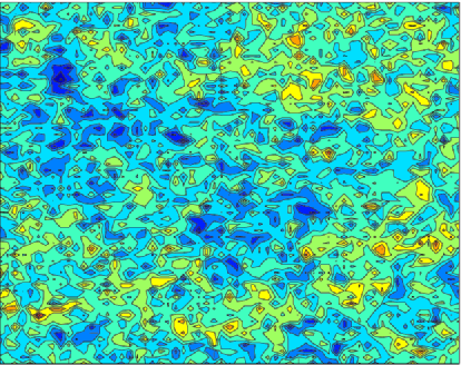
Figure 1: Height landscape of the derivative martingale measure plotted with a logarithmic scale color-bar, showing that the measure is very “peaked” (for $t=12$, a multiplicative factor of about $10^{8}$ stands between extreme values, i.e., between warm and cold colors).

In a sense, the measures $M^{\gamma}$ in (1) become more concentrated as $\gamma^{2}$ approaches $2d$. (They assign full measure to a set of Hausdorff dimension $d-\gamma^{2}/2$, which tends to zero as $\gamma^{2}\to 2d$.) It is therefore natural to wonder how concentrated the $\gamma^{2}=2d$ measure will be (see Figure 1 for a simulation of the landscape). In particular, it is natural to wonder whether it possesses atoms (in which case it could in principle assign full measure to a countable set). In our context, we will answer in the negative. At the time we posted the first version of this manuscript online, this question was open in the context of discrete models as well as continuous models. However, a proof of the nonatomicity of the discrete cascade measures was posted very shortly afterward in BKNSW , which uses a method independent of our proof. Since our proof is based on a continuous version of the spine decomposition, as developed in the context of branching random walks, we expect that it can be adapted to these other models as well.

Roughly speaking, the reason that establishing nonatomicity in critical models is nontrivial is that proofs of nonatomicity for (noncritical) multiplicative chaos usually rely on the existence of moments higher than $1$ (see daley ) and the scaling relations of multifractal random measures; see, for example, allez . At criticality, the random measures involved (cascades, branching random walks, or Gaussian multiplicative chaos) no longer possess finite moments of order $1$, and the scaling relations become useless.

To explain this issue in more detail, we recall that it is proved in daley that a stationary random measure $M$ over $\mathbb{R}^{d}$ is almost surely nonatomic if ($C$ stands here for the unit cube of $\mathbb{R}^{d}$)

$$\forall\delta>0\qquad n^{d}\mathbb{P}\bigl{(}M\bigl{(}{n}^{-1}C\bigr{)}>\delta\bigr{)}\to 0\qquad\mbox{as }n\to\infty.$$ (3)

When $M=M_{\gamma}$ for $0<\gamma^{2}<2d$, a computable property of $M_{\gamma}$ is its power-law spectrum $\xi$ characterized by

$$\mathbb{E}\bigl{[}\bigl{(}M^{\gamma}\bigl{(}{n}^{-1}C\bigr{)}\bigr{)}^{q}\bigr{]}\simeq D_{q}{n^{-\xi(q)}}\qquad\mbox{as }n\to\infty$$ (4)

for all those $q$ making the above expectation finite, that is, $q\in[0,\frac{2d}{\gamma^{2}}[$. It matches

$$\xi(q)=\biggl{(}d+\frac{\gamma^{2}}{2}\biggr{)}q-\frac{\gamma^{2}}{2}q^{2}.$$ (5)

Using the Markov inequality in (3), (4) obviously yields for $q\in[0,\frac{2d}{\gamma^{2}}[$

$$n^{d}\mathbb{P}\bigl{(}M^{\gamma}\bigl{(}{n}^{-1}C\bigr{)}>\delta\bigr{)}\lesssim\frac{D_{q}}{\delta^{q}}n^{d-\xi(q)}.$$

Therefore, the nonatomicity of the measure boils down to finding a $q$ such that the power-law spectrum is strictly larger than $d$:

• In the subcritical situation $\gamma^{2}<2d$, the function $\xi$ increases on $[0,1]$ from $0$ to $d$. Such a $q$ is necessarily larger than $1$, and a straightforward computation shows that any $q\in\,]1,\frac{2d}{\gamma^{2}}[$ suffices.

• For $\gamma^{2}=2d$, relations (4) and (5) should remain valid only for $q<1$. Therefore, the subcritical strategy fails because the power-law spectrum achieves its maximum $d$ at $q=1$. It is tempting to try to replace the gauge function $x\mapsto x^{q}$ by something that could be more appropriate at criticality like $x\mapsto x\ln(1+x)^{q}$, etc. However, the fact that the measure does not possess a moment of order $1$ (see Proposition 5 below) shows that there is no way of changing the gauge so as to make $\xi$ go beyond $d$.

More sophisticated machinery is thus necessary to investigate nonatomicity at criticality. Indeed, we expect the derivative martingale to assign full measure to a (random) Hausdorff set of dimension $0$, indicating that the measure is in some sense just “barely” nonatomic.

Let us finally mention the interesting work of tecu where the author constructs on the unit circle ($d=1$) a classical Gaussian multiplicative Chaos given by the exponential of a field $X$ such that for each $\varepsilon$ the covariance of $X$ at points $x$ and $y$ lies strictly between $(2-\varepsilon)\ln_{+}\frac{1}{|x-y|}$ and $2\ln_{+}\frac{1}{|x-y|}$ when $|x-y|$ is sufficiently small. In some sense, his construction is a near critical construction, different from the measures constructed here. This is illustrated by the fact that the measures in tecu possess moments of order $1$ (and even belong to $L\log L$), which is atypical for the critical multiplicative chaos associated to log-correlated random variables.

In this paper, we tackle the problem of constructing random measures at criticality for a large class of log-correlated Gaussian fields in any dimension, the covariance kernels of which are called $\star$-scale invariant kernels. This approach allows us to link the measures under consideration to a functional equation, the $\star$-equation, giving rise to several conjectures about the glassy phase of log-correlated Gaussian potentials and about the three-terms expansion of the maximum of log-correlated Gaussian variables.

Another important family of random measures is the class defined by taking $X$ to be the Gaussian Free Field (GFF) with free or Dirichlet boundary conditions on a planar domain, as in cfDuSh ; see also She07 for an introduction to the GFF. The measures defined in this way are also known as the (critical) Liouville quantum gravity measures, and are closely related to conformal field theory, as well as various 2-dimensional discrete random surface models and their scaling limits. Although the Gaussian free field is in some sense a log-correlated random field, it does not fall exactly into the framework of this paper, which deals with translation invariant random measures (defined on all of $\mathbb{R}^{2}$ or $\mathbb{R}^{d}$) that can be approximated in a particular way (via the $\star$-equation). Although some of the arguments of this paper can be easily extended to settings where the strict translation invariance requirement for $X$ is relaxed (e.g., $X$ is the Gaussian free field on a disk), we will still need additional arguments to show that the derivative martingale associates a unique nonatomic random positive measure to a given instance of the GFF almost surely, that this measure is independent of the particular approximation scheme used, and that this measure transforms under conformal maps in the same way as the $\gamma<2$ measures constructed in cfDuSh . For the sake of pedagogy, this other part of our work will appear in a companion paper. For the time being, we just announce that all the results of this paper are valid for the GFF construction.

1.2 Physics literature: History and motivation

It is interesting to pause for a moment and consider the physics literature on Liouville quantum gravity. We first remark that the noncritical case, with $d=2$ and $\gamma<2$, was treated in cfDuSh , which contains an extensive overview of the physics literature and an explanation of the relationships (some proved, some conjectural) between random measures and discrete and continuum random surfaces. Roughly speaking, when one takes a random two-dimensional manifold and conformally maps it to a disk, the image of the area measure is a random measure on the disk that should correspond to an exponential of a log-correlated Gaussian random variable (some form of the GFF). From this point of view, many of the physics results about discrete and continuum random surfaces can be interpreted as predictions about the behavior of these random measures, where the value of $\gamma<2$ depends on the particular physical model in question.

There is also a physics literature focusing on the critical case $\gamma=2$, which we expect to be related to the measure constructed in this paper. This section contains a brief overview of the results from this literature, as appearing in, for example, BKZ , GM , GZ , GrossKleban , GrossM , GubserKleban , KKK , Kleb2 , kostov91 , kostov92 , KS , Parisi , Polch , sugino . Most of the results surveyed in this section have not yet been established or understood in a mathematical sense.

The critical case $\gamma=2$ corresponds to the value $c=1$ of the so-called central charge $c$ of the conformal field theory coupled to gravity, via the famous KPZ result cfKPZ ,

$$\gamma=\frac{1}{\sqrt{6}}(\sqrt{25-c}-\sqrt{1-c}).$$

Discrete critical statistical physical models having $c=1$ then include one-dimensional matrix models [also called “matrix quantum mechanics” (MQM)] BKZ , GM , GZ , GrossKleban , GubserKleban , KKK , Kleb2 , Parisi , Polch , sugino , the so-called $O(n)$ loop model on a random planar lattice for $n=2$ kostov91 , kostov92 , Kostovhouches , KS and the $Q$-state Potts model on a random lattice for $Q=4$ BBM , Daul , Ey . For an introduction to the above mentioned 2D statistical models, see, for example, Nienhuis .

In the continuum, a natural coupling also exists between Liouville quantum gravity and the Schramm–Loewner evolution SLE_κ for $\gamma=\sqrt{\kappa}$, rigorously established for $\kappa<4$ PRL1 , She11 . Thus the critical value $\gamma=2$ corresponds to the special SLE parameter value $\kappa=4$, above which the SLE_κ curve no longer is a simple curve, but develops double points at all scales.

The standard $c=1,\gamma=2$ Liouville field theory BKZ , GM , GZ , GrossKleban , KKK , Kleb2 , Parisi , Polch involves violations of scaling by logarithmic factors. For example, the partition function (number) of genus $0$ random surfaces of area $\mathcal{A}$ grows as GrossKleban , KKK

$$\mathcal{Z}\propto\exp(\mu\mathcal{A})\mathcal{A}^{-3}(\log\mathcal{A})^{-2},$$

where $\mu$ is a nonuniversal growth constant depending on the (planar lattice) regularization. The area exponent ($-$3) is universal for a $c=1$ central charge, while the subleading logarithmic factor is attributed to the unusual dependence on the Liouville field $\varphi$ (equivalent to $X$ here) of the so-called “tachyon field” $T(\varphi)\propto\varphi e^{2\varphi}$ KKK , Kleb2 , Polch . Its integral over a “background” Borelian set $A$ generates the quantum area $\mathcal{A}=\int_{A}T(\varphi)\,dx$, that we can recognize as the formal heuristic expression for the derivative measure (1.1) introduced above.

At $c=1$, a proliferation of large “bubbles” (the so-called “baby universes” which are relatively large amounts of area cut off by relatively small bottlenecks) is generally anticipated in the bulk of the random surface GrossKleban , Jain , kostov91 , or at its boundary in the case of a disk topology kostov92 , KS . We believe that this should correspond to the fact that the measure we construct is concentrated on a set of Hausdorff dimension zero.

However, the introduction of higher trace terms GubserKleban , Kleb2 , sugino in the action of the $c=1$ matrix model of two-dimensional quantum gravity is known to generate a “nonstandard” random surface model with an even stronger concentration of bottlenecks. (See also the related detailed study of a MQM model for a $c=1$ string theory with vortices in KKK .) As we shall see shortly, these nonstandard constructions do not seem to correspond to our model, at least not so directly. In these constructions, one encounters a new critical behavior of the random surface, with a critical proliferation of spherical bubbles connected one to another by microscopic “wormholes.” This is reminiscent of the construction for $c<1,\gamma<2$ of the dual phase of Liouville quantum gravity Al , Amb , Das , Dur , Kleb1 , Kleb2 , Kleb3 , where the associated random measure develops atoms BJRV , Duphouches , PRL .

The partition function of the nonstandard $c=1$ (genus zero) random surface then scales as a function of the area $\mathcal{A}$ as GubserKleban , KKK , Kleb2 , sugino

$$\mathcal{Z}\propto\exp\bigl{(}\mu^{\prime}\mathcal{A}\bigr{)}\mathcal{A}^{-3}$$

with an apparent suppression of logarithmic terms. This has been attributed to the appearance for $c=1$ of a tachyon field of the atypical form $T(\varphi)\propto e^{2\varphi}$ GubserKleban , KKK , Kleb3 . Heuristically, this would seem to correspond to a measure of type (1), but we know that the latter vanishes for $\gamma=2$. (See Proposition 19 below.) The literature about the analogous problem of branching random walks AidShi , HuShi also suggests for $\gamma=2$ a logarithmically renormalized measure obtained by multiplying by $\sqrt{\log(1/\varepsilon)}=\sqrt{t}$ the object [see (7) below] whose limit is taken in (1), but we expect this to converge (up to constant factor) to the same measure as the derivative martingale (1.1). In order to model the nonstandard theory, it might be necessary to modify the measures introduced here by explicitly introducing “atoms” on top of them, using the procedure described in BJRV , Duphouches , PRL for adding atoms to $\gamma<2$ random measures. In the approach of BJRV , Duphouches , PRL , the “dual Liouville measure” corresponding to $\gamma<2$ involves choosing a Poisson point process from $\eta^{-\alpha-1}\,d\eta M_{\gamma}(dx)$, where $\alpha=\gamma^{2}/4\in(0,1)$, and letting each point $(\eta,x)$ in this process indicate an atom of size $\eta$ at location $x$. When $\gamma=2$ and $\alpha=1$, we can replace $M_{\gamma}$ with the $M^{\prime}$ of (1.1) and use the same construction; in this case (since $\alpha=1$) the measure a.s. assigns infinite mass to each positive-Lebesgue-measure $A\in\mathcal{B}(\mathbb{R}^{d})$. However, one may use standard Lévy compensation to produce a random distribution, assigning a finite value a.s. to each fixed $A\in\mathcal{B}(\mathbb{R}^{d})$ with a positive atom of size $\eta$ at location $x$ corresponding to each $(\eta,x)$ in the Poisson point process. We suspect that that this construction is somehow equivalent to the continuum random measure associated with the nonstandard $c=1,\gamma=2$ Liouville random surface with enhanced bottlenecks, as described in GubserKleban , KKK , sugino .

Finally, we note that the boundary critical Liouville quantum gravity poses similar challenges. A subtle difference in logarithmic boundary behavior is predicted between the so-called dilute and dense phases of the $O(2)$ model on a random disk kostov92 , KS , which thus may differ in their boundary bubble structure. It also remains an open question whether the results about the conformal welding of two boundary arcs of random surfaces to produce SLE, as described in She11 , can be extended to the case $\gamma=2$.

2 Setup

2.1 Notation

For a Borelian set $A\subset\mathbb{R}^{d}$, $\mathcal{B}(A)$ stands for the Borelian sigma-algebra on $A$. All the considered fields are constructed on the same probability space $(\Omega,\mathcal{F},\mathbb{P})$. We denote by $\mathbb{E}$ the corresponding expectation.

2.2 $\star$-scale invariant kernels

Here we introduce the Gaussian fields that we will use throughout the papers. We consider a family of centered stationary Gaussian processes $((X_{t}(x))_{x\in\mathbb{R}^{d}})_{t\geq 0}$ where, for each $t\geq 0$, the process $(X_{t}(x))_{x\in\mathbb{R}^{d}}$ has covariance given by

$$K_{t}(x)=\mathbb{E}\bigl{[}X_{t}(0)X_{t}(x)\bigr{]}=\int_{1}^{e^{t}}\frac{k(ux)}{u}\,du$$ (6)

for some covariance kernel $k$ satisfying $k(0)=1$, of class $C^{1}$ and vanishing outside a compact set (actually this latter condition is not necessary but it simplifies the presentation). The $C^{1}$ condition is technical and ensures that for $x\neq y$ we have a nice description of the joint law of the couple $(X_{t}(x),X_{t}(y))_{t\geq 0}$; see Lemma 16 below (this condition could also be relaxed to some extent). We also assume that the process $(X_{t}(x)-X_{s}(x))_{x\in\mathbb{R}^{d}}$ is independent of the processes $((X_{u}(x))_{x\in\mathbb{R}^{d}})_{u\leq s}$ for all $s<t$. Put in other words, the mapping $t\mapsto X_{t}(\cdot)$ has independent increments. Such a construction of Gaussian processes is carried out in allez . For $\gamma\geq 0$, we consider the approximate Gaussian multiplicative chaos $M^{\gamma}_{t}(dx)$ on $\mathbb{R}^{d}$,

$$M^{\gamma}_{t}(dx)=e^{\gamma X_{t}(x)-(\gamma^{2}/2)E[X_{t}(x)^{2}]}\,dx.$$ (7)

It is well known allez , cfKah that, almost surely, the family of random measures $(M^{\gamma}_{t})_{t>0}$ weakly converges as $t\to\infty$ toward a random measure $M^{\gamma}$, which is nontrivial if and only if $\gamma^{2}<2d$. The purpose of this paper is to investigate the phase transition, that is, $\gamma^{2}=2d$. Recall that we have:

Proposition 1.

For $\gamma^{2}=2d$, the standard construction (7) yields a vanishing limiting measure

$$\lim_{t\to\infty}M^{\sqrt{2d}}_{t}(dx)=0\qquad\mbox{almost surely}.$$ (8)

Let us also mention that the authors in allez have proved that, for $\gamma^{2}<2d$, the measure $M^{\gamma}$ satisfies the following scale invariance relation, called $\star$-equation:

Definition 2 ((Log-normal $\star$-scale invariance)).

The random Radon measure $M^{\gamma}$ is lognormal $\star$-scale invariant: for all $0<\varepsilon\leq 1$, $M^{\gamma}$ obeys the cascading rule

$$\bigl{(}M^{\gamma}(A)\bigr{)}_{A\in\mathcal{B}(\mathbb{R}^{d})}$$

(9)

$$\qquad\stackrel{{\scriptstyle\mathrm{law}}}{{=}}\biggl{(}\int_{A}e^{\gamma X_{\ln(1/\varepsilon)}(r)-(\gamma^{2}/2)\mathbb{E}[X_{\ln(1/\varepsilon)}(r)^{2}]}\varepsilon^{d}M^{\gamma,\varepsilon}(dr)\biggr{)}_{A\in\mathcal{B}(\mathbb{R}^{d})},$$

where $X_{\ln(1/\varepsilon)}$ is the Gaussian process introduced in (6), and $M^{\gamma,\varepsilon}$ is a random measure independent from $X_{\ln(1/\varepsilon)}$ satisfying the scaling relation

$$\bigl{(}M^{\gamma,\varepsilon}(A)\bigr{)}_{A\in\mathcal{B}(\mathbb{R}^{d})}\stackrel{{\scriptstyle\mathrm{law}}}{{=}}\biggl{(}M^{\gamma}\biggl{(}\frac{A}{\varepsilon}\biggr{)}\biggr{)}_{A\in\mathcal{B}(\mathbb{R}^{d})}.$$ (10)

Intuitively, this relation means that when zooming in the measure $M$, one should observe the same behavior up to an independent Gaussian factor. It has some canonical meaning since it is the exact continuous analog of the smoothing transformation intensively studied in the context of Mandelbrot’s multiplicative cascades durrett or branching random walks Biggf , Liu .

Observe that this equation perfectly makes sense for the value $\gamma^{2}=2d$. Therefore, to define a natural Gaussian multiplicative chaos at the value $\gamma^{2}=2d$, one has to look for a solution to this equation when $\gamma^{2}=2d$ and conversely, each random measure candidate for being a Gaussian multiplicative chaos at the value $\gamma^{2}=2d$ must satisfy this equation.

Remark 3.

The main motivation for considering $\star$-scale invariant kernels is the connection between the associated random measures and the $\star$-equation. Nevertheless, we stress that our proofs can be easily adapted to other Gaussian multiplicative chaos associated to log-correlated Gaussian fields “à la Kahane” cfKah : in particular, we can construct the derivative martingale associated to exact scale invariant kernels bacry , rhovar or the Gaussian Free Field in a bounded domain.

3 Derivative martingale

One way to construct a solution to the $\star$-equation at the critical value $\gamma^{2}=2d$ is to introduce the derivative martingale $M_{t}^{\prime}(dx)$ defined by

$$M_{t}^{\prime}(dx) := \bigl{(}\sqrt{2d}t-X_{t}(x)\bigr{)}e^{\sqrt{2d}X_{t}(x)-d\mathbb{E}[X_{t}(x)^{2}]}\,dx.$$

It is plain to see that, for each open bounded set $A\subset\mathbb{R}^{d}$, the family $(M_{t}^{\prime}(A))_{t}$ is a martingale. Nevertheless, it is not nonnegative. It is therefore not obvious that such a family converges toward a (nontrivial) positive limiting random variable. The following theorem is the main result of this section:

Theorem 4

For each bounded open set $A\subset\mathbb{R}^{d}$, the martingale$(M^{\prime}_{t}(A))_{t\geq 0}$ converges almost surely toward a positive random variable denoted by $M^{\prime}(A)$, such that $M^{\prime}(A)>0$ almost surely. Consequently, almost surely, the (locally signed) random measures $(M^{\prime}_{t}(dx))_{t\geq 0}$ converge weakly as $t\to\infty$ toward a positive random measure $M^{\prime}(dx)$. This limiting measure has full support and is atomless. Furthermore, the measure $M^{\prime}$ is a solution to the $\star$-equation (2) with $\gamma=\sqrt{2d}$.

Since $M_{t}^{\prime}(dx)$ is not uniformly nonnegative when $t<\infty$, there are several complications involved in establishing its convergence to a nonnegative limit (let alone the nontriviality of the limit). We have to introduce some further tools to study its convergence. These tools have already been introduced in the context of discrete multiplicative cascade models in order to study the corresponding derivative martingale; see BiKi .

We denote by $\mathcal{F}_{t}$ the sigma algebra generated by $\{X_{s}(x);s\leq t,x\in\mathbb{R}^{d}\}$. Given a Borelian set $A\subset\mathbb{R}^{d}$ and parameters $t,\beta>0$, we introduce the random variables

$$Z^{\beta}_{t}(A) = \int_{A}\bigl{(}\sqrt{2d}t-X_{t}(x)+\beta\bigr{)}\mathbh{1}_{\{\tau^{\beta}>t\}}e^{\sqrt{2d}X_{t}(x)-d\mathbb{E}[X_{t}(x)^{2}]}\,dx,$$

$$\widetilde{Z}^{\beta}_{t}(A) = \int_{A}\bigl{(}\sqrt{2d}t-X_{t}(x)\bigr{)}\mathbh{1}_{\{\tau^{\beta}>t\}}e^{\sqrt{2d}X_{t}(x)-d\mathbb{E}[X_{t}(x)^{2}]}\,dx,$$

where, for each $x\in A$, $\tau^{\beta}(x)$ is the $(\mathcal{F}_{t})_{t}$-stopping time defined by

$$\tau^{\beta}(x)=\inf\bigl{\{}u>0,X_{u}(x)-\sqrt{2d}u>\beta\bigr{\}}.$$

In the sequel, when the context is clear, we will drop the $x$ dependence in $\tau^{\beta}(x)$. What is the relation between $Z^{\beta}_{t}(A)$ and $M_{t}^{\prime}(A)$? Roughly speaking, we will show that the convergence of $M^{\prime}_{t}(A)$ as $t\to\infty$ toward a nontrivial object boils down to proving the convergence of $Z^{\beta}_{t}(A)$ toward a nontrivial object: we will prove that the difference $Z^{\beta}_{t}(A)-\widetilde{Z}^{\beta}_{t}(A)$ almost surely goes to $0$ as $t\to\infty$ and that $\widetilde{Z}^{\beta}_{t}(A)$ coincides with $M_{t}^{\prime}(A)$ for $\beta$ large enough. In particular, we will prove that $Z^{\beta}_{t}(A)$ converges toward a random variable $Z^{\beta}(A)$ which itself converges as $\beta\to\infty$ to the limit of $M_{t}^{\prime}(A)$ (as $t\to\infty$). The details and proofs are gathered in the Appendix.

As a direct consequence of our method of proof, we get the following properties of $M^{\prime}(dx)$:

Proposition 5.

The positive random measure $M^{\prime}(dx)$ possesses moments of order $q$ for all $q\leq 0$. It does not possess moments of order $1$.

As a direct consequence of the fact that the measure $M^{\prime}$ satisfies the $\star$-equation, it possesses moments of order $q$ for all $q\leq 0$. This is a straightforward adaptation of the corresponding theorem in Barral1 ; see also Benj for a proof in English. Since $Z^{\beta}(dx)$ increases toward $M^{\prime}$ as $\beta$ goes to infinity, we have $M^{\prime}(dx)\geq Z^{\beta}(dx)$ for any $\beta$. Since $Z^{\beta}_{t}$ is a uniformly integrable martingale, we have $\mathbb{E}[Z^{\beta}(A)]=\mathbb{E}[Z^{\beta}_{0}(A)]=\beta|A|$, we deduce that $\mathbb{E}[M^{\prime}(A)]=+\infty$ for every bounded open set $A$.

4 Conjectures

In this section, we present a few results we can prove about the $\star$-equation and some conjectures related to these results.

4.1 About the $\star$-equation

Consider the $\star$-equation in great generality, that is:

Definition 6 ((Log-normal $\star$-scale invariance)).

A random Radon measure $M$ is lognormal $\star$-scale invariant if for all $0<\varepsilon\leq 1$, $M$ obeys the cascading rule

$$\bigl{(}M(A)\bigr{)}_{A\in\mathcal{B}(\mathbb{R}^{d})}\stackrel{{\scriptstyle\mathrm{law}}}{{=}}\biggl{(}\int_{A}e^{\omega_{\varepsilon}(r)}M^{\varepsilon}(dr)\biggr{)}_{A\in\mathcal{B}(\mathbb{R}^{d})},$$ (11)

where $\omega_{\varepsilon}$ is a stationary stochastically continuous Gaussian process, and $M^{\varepsilon}$ is a random measure independent from $\omega_{\varepsilon}$ satisfying the scaling relation

$$\bigl{(}M^{\varepsilon}(A)\bigr{)}_{A\in\mathcal{B}(\mathbb{R}^{d})}\stackrel{{\scriptstyle\mathrm{law}}}{{=}}\biggl{(}M\biggl{(}\frac{A}{\varepsilon}\biggr{)}\biggr{)}_{A\in\mathcal{B}(\mathbb{R}^{d})}.$$ (12)

Observe that, in comparison with (2) and (10), we do not require the scaling factor to be $\varepsilon^{d}$. As stated in (11) and (12), it is proved in allez that $\mathbb{E}[e^{\omega_{\varepsilon}(r)}]=\varepsilon^{d}$ as soon as the measure possesses a moment of order $1+\delta$ for some $\delta>0$. Roughly speaking, it remains to investigate situations when the measure does not possess a moment of order $1$, and we will see that the scaling factor is then not necessarily $\varepsilon^{d}$.

Inspired by the discrete multiplicative cascade case (see durrett ), our conjecture is that all the nontrivial short ranged solutions [i.e., there exists $R>0$ such that $M(A)$ and $M(B)$ are independent when $d(A,B)\geq R$ where $d$ is the standard distance between sets] to this equation belong to one of the families we will describe below.

First we conjecture that there exists a $\alpha\in\,]0,1]$ such that

$$\mathbb{E}\bigl{[}e^{\alpha\omega_{\varepsilon}(r)}\bigr{]}=\varepsilon^{d}.$$

Assuming this, it is proved in allez , sohier that the Gaussian process $\alpha\omega_{e^{-t}}$ has a covariance structure given by (6). More precisely, there exists some compactly supported continuous covariance kernel $k$ with $k(0)=1$ and $\gamma^{2}\leq 2d$ such that

$$\operatorname{Cov}\bigl{(}\alpha\omega_{e^{-t}}(0),\alpha\omega_{e^{-t}}(x)\bigr{)}=\gamma^{2}\int_{1}^{e^{t}}\frac{k(ux)}{u}\,du.$$

We can then rewrite the process $\omega$ as

$$\omega_{e^{-t}}(x)=\frac{\gamma}{\alpha}X_{t}(x)-\frac{\gamma^{2}}{2\alpha}t-\frac{d}{\alpha}t,$$

where $(X_{t})_{t}$ is the family of Gaussian fields introduced in Section 2. We now consider four cases, depending on the values of $\alpha$ and $\gamma$ [cases (2), (3), (4) are conjectures]:

[(4)]

If $\alpha=1$ and $\gamma^{2}<2d$, then the law of the solution $M$ is the standard Gaussian multiplicative chaos $M^{\gamma}$ [see (7)] up to a multiplicative constant. This case has been treated in allez .

If $\alpha=1$ and $\gamma^{2}=2d$, then the law of the solution $M$ is that of the derivative martingale that we have constructed in this paper (Theorem 4), up to a multiplicative constant.

If $\alpha<1$ and $\gamma^{2}<2d$, then $M$ is an atomic Gaussian multiplicative chaos as constructed in BJRV up to a multiplicative constant. More precisely, the law can be constructed as follows:

1. [(a)]

2. Sample a standard Gaussian multiplicative chaos

   $$\overline{M}(dx)=e^{\gamma X(x)-(\gamma^{2}/2)\mathbb{E}[X(x)^{2}]}\,dx.$$

   The measure $\overline{M}$ is perfectly defined since $\gamma^{2}<2d$.

3. Sample an independently scattered random measure $N$ whose law, conditioned on $\overline{M}$, is characterized by

   $$\forall q\geq 0\qquad\mathbb{E}\bigl{[}e^{-qN(A)}|\overline{M}\bigr{]}=e^{-q^{\alpha}\overline{M}(A)}.$$

   Then the law of $M$ is that of $N$ up to a multiplicative constant.

If $\alpha<1$ and $\gamma^{2}=2d$, then $M$ is an atomic Gaussian multiplicative chaos of a new type. More precisely, the law can be constructed as follows:

1. [(a)]

2. Sample the derivative Gaussian multiplicative chaos

   $$M^{\prime}(dx)=\bigl{(}\sqrt{2d}\mathbb{E}\bigl{[}X(x)^{2}\bigr{]}-X(x)\bigr{)}e^{\sqrt{2d}X(x)-d\mathbb{E}[X(x)^{2}]}\,dx.$$

   The measure $M^{\prime}$ is constructed as prescribed by Theorem 4.

3. Sample an independently scattered random measure $N$ whose law, conditioned on $M^{\prime}$, is characterized by

   $$\forall A\in\mathcal{B}\bigl{(}\mathbb{R}^{d}\bigr{)},\ \forall q\geq 0\qquad\mathbb{E}\bigl{[}e^{-qN(A)}|M^{\prime}\bigr{]}=e^{-q^{\alpha}M^{\prime}(A)}.$$

   Then the law of $M$ is that of $N$ up to a multiplicative constant.

Notice that the results of our paper together with allez , BJRV allow us to prove existence of all the random measures described above. Therefore, it remains to complete the uniqueness part of this statement.

Remark 7.

The $\alpha<1,\gamma^{2}<2d$ case above has been used in BJRV , Duphouches , PRL to give a mathematical understanding of the duality in Liouville quantum gravity: this corresponds to taking special values of the couple $(\alpha,\gamma)$. More precisely, we choose some parameter $\bar{\gamma}^{2}>2d$. If the measure $M_{\bar{\gamma}}$ was well defined, it would satisfy the scaling relation

$$\bigl{(}M_{\bar{\gamma}}(A)\bigr{)}_{A\in\mathcal{B}(\mathbb{R}^{d})}$$

(13)

$$\qquad\stackrel{{\scriptstyle\mathrm{law}}}{{=}}\biggl{(}\int_{A}e^{\bar{\gamma}X_{\ln(1/\varepsilon)}(r)-(\bar{\gamma}^{2}/2)\mathbb{E}[X_{\ln(1/\varepsilon)}(r)^{2}]}\varepsilon^{d}M^{\bar{\gamma},\varepsilon}(dr)\biggr{)}_{A\in\mathcal{B}(\mathbb{R}^{d})},$$

where $M^{\bar{\gamma},\varepsilon}$ is a random measure independent from $X_{\varepsilon}$ satisfying the scaling relation

$$\bigl{(}M^{\bar{\gamma},\varepsilon}(A)\bigr{)}_{A\in\mathcal{B}(\mathbb{R}^{d})}\stackrel{{\scriptstyle\mathrm{law}}}{{=}}\biggl{(}M^{\bar{\gamma}}\biggl{(}\frac{A}{\varepsilon}\biggr{)}\biggr{)}_{A\in\mathcal{B}(\mathbb{R}^{d})}.$$ (14)

Nevertheless, we know that $M^{\bar{\gamma}}$ yields a vanishing measure. The idea is thus to use the $\star$-equation to determine what the unique solution of this scaling relation is. Writing $\gamma=\frac{2d}{\bar{\gamma}}<2d$ and $\alpha=\frac{2d}{\bar{\gamma}^{2}}$, it is plain to see that

$$\mathbb{E}\bigl{[}\bigl{(}e^{\bar{\gamma}X_{\ln(1/\varepsilon)}(r)-(\bar{\gamma}^{2}/2)\mathbb{E}[X_{\ln(1/\varepsilon)}(r)^{2}]}\varepsilon^{d}\bigr{)}^{\alpha}\bigr{]}=\varepsilon^{d}.$$

Therefore, we are in situation 3, which yields a natural candidate for Liouville duality BJRV , Duphouches , PRL .

4.2 Another construction of solutions to the critical $\star$-equation

Recall that the measures $M^{\gamma}$ for $\gamma<2$ are obtained as limits of (1) as $X$ varies along approximations to a limit field. The measure constructed in Theorem 4 is defined analogously except that one replaces (1) with (1.1), which is minus the derivative of (1) at $\gamma=\sqrt{2d}$. If we could exchange the order of the differentiation and the limit-taking, we would conclude that the measure constructed in Theorem 4 is equal to

$$-\frac{\partial}{\partial\gamma}\bigl{[}M^{\gamma}\bigr{]}_{\gamma=\sqrt{2d}}=\lim_{\gamma\to\sqrt{2d}}\frac{1}{\sqrt{2d}-\gamma}M^{\gamma}.$$

We will not fully justify this order exchange here, but we will establish a somewhat weaker result. Namely, we show that one can at least obtain some solution to the $\star$-equation as a limit of this general type. This construction is inspired by a similar construction for discrete multiplicative cascades in durrett . More precisely, we have the following (proved in Section A.2):

Proposition 8.

There exist two increasing sequence $(\lambda_{n})_{n}$ and $(\gamma_{n})_{n}$, with $\gamma_{n}^{2}<2d$ and $\gamma_{n}^{2}\to 2d$ as $n\to\infty$, such that

$$\lambda_{n}M^{\gamma_{n}}(dx)\stackrel{{\scriptstyle\mathrm{law}}}{{\to}}M^{c}(dx),$$

where $M^{c}$ is a positive random measure satisfying (2).

The following conjecture is a consequence of the uniqueness conjecture for the $\star$-equation exposed in Section 4.1 above:

Conjecture 9.

The construction of Proposition 8 gives the same measure as the one described in Section 3 (up to some multiplicative constant). Moreover, the sequence $(\lambda_{n})_{n}$ can be chosen as $\lambda_{n}=\frac{1}{\sqrt{2d}-\gamma_{n}}$ (in dimension $d$).

4.3 Glassy phase of log-correlated Gaussian potentials

The glassy phase of log-correlated Gaussian potentials is concerned with the behavior of measures beyond the critical value $\gamma^{2}>2d$. More precisely, for $\gamma^{2}>2d$, consider the measure

$$M^{\gamma}_{t}(dx)=e^{\gamma X_{t}(x)-(\gamma^{2}/2)\mathbb{E}[X_{t}(x)^{2}]}\,dx.$$

The limiting measure, as $t\to\infty$, vanishes as proved in cfKah . Therefore, it is natural to look for a suitable family of normalizing factors to make this measure converge. With the arguments used in Section B.1 to compare with the results obtained in BRV , madaule , we can rigorously prove:

Proposition 10.

The renormalized family

$$\bigl{(}t^{(3\gamma)/(2\sqrt{2d})}e^{t((\gamma/\sqrt{2})-\sqrt{d})^{2}}M^{\gamma}_{t}(dx)\bigr{)}_{t\geq 0}$$

is tight. Furthermore, every converging subsequence is nontrivial.

The above proposition can be obtained using the results in BRV , madaule and Section B.1 (tightness statement). The main result in bramson about the behavior of the maximum of the discrete GFF implies that every converging subsequence is nontrivial.

We now formulate a conjecture about the limiting law of this family. Assuming that the above renormalized family converges in law (so we strengthen tightness into convergence), it turns out that the limit $M^{\gamma}$ of this renormalized family necessarily satisfies the following $\star$-equation:

$$M^{\gamma}(dx)=e^{\gamma X_{\ln(1/\varepsilon)}(x)-\sqrt{(d/2)}\gamma\mathbb{E}[X_{\ln(1/\varepsilon)}(x)^{2}]}\varepsilon^{\sqrt{(d/2)}\gamma}\overline{M}^{\gamma}\biggl{(}\frac{dx}{\varepsilon}\biggr{)},$$

where $\overline{M}^{\gamma}$ is a random measure with the same law as $M^{\gamma}$ and independent of the process $(X_{t}(x))_{x\in\mathbb{R}^{d}}$. Setting $\alpha=\frac{\sqrt{2d}}{\gamma}\in\,]0,1[$, this equation can be rewritten as

$$M^{\gamma}(dx)=e^{(\sqrt{2d}/\alpha)X_{\ln(1/\varepsilon)}(x)-(d/\alpha)\mathbb{E}[X_{\ln(1/\varepsilon)}(x)^{2}]}\varepsilon^{d/\alpha}\overline{M}^{\gamma}\biggl{(}\frac{dx}{\varepsilon}\biggr{)}.$$

Therefore, assuming that the conjectures about uniqueness of the $\star$-equation are true, we have the following:

Conjecture 11.

$$t^{(3\gamma)/(2\sqrt{2d})}e^{t((\gamma/\sqrt{2})-\sqrt{d})^{2}}M^{\gamma}_{t}(dx)\stackrel{{\scriptstyle\mathrm{law}}}{{\to}}c_{\gamma}N_{\alpha}(dx)\qquad\mbox{as }t\to\infty,$$ (15)

where $c_{\gamma}$ is a positive constant depending on $\gamma$ and the law of $N_{\alpha}$ is given, conditioned on the derivative martingale $M^{\prime}$, by an independently scattered random measure the law of which is characterized by

$$\forall A\in\mathcal{B}\bigl{(}\mathbb{R}^{d}\bigr{)},\ \forall q\geq 0\qquad\mathbb{E}\bigl{[}e^{-qN_{\alpha}(A)}|M^{\prime}\bigr{]}=e^{-q^{\alpha}M^{\prime}(A)}.$$

In particular, physicists are interested in the behavior of the Gibbs measure associated to $M^{\gamma}_{t}(dx)$ on a ball $B$. It is the measure renormalized by its total mass,

$$G^{\gamma}_{t}(dx)=\frac{M^{\gamma}_{t}(dx)}{M^{\gamma}_{t}(B)}.$$

From (15), we deduce

$$G^{\gamma}_{t}(dx)\stackrel{{\scriptstyle\mathrm{law}}}{{\to}}\frac{N_{\alpha}(dx)}{N_{\alpha}(B)}\qquad\mbox{as }t\to\infty.$$ (16)

The size reordered atoms of the latter object form a Poisson–Dirichlet process as conjectured by physicists CarDou and proved rigorously in arguin . Nevertheless, we point out that this conjecture is more powerful than the Poisson–Dirichlet result since it also makes precise the spatial localization of the atoms. We stress that this result has been proved in the case of branching random walks BRV , built on the work of Madaule madaule .

4.4 About the maximum of the log-correlated Gaussian random variables

It is proved in bramson (in fact $d=2$ in bramson but this is general) that the family

$$\biggl{(}\sup_{x\in[0,1]^{d}}X_{t}(x)-\sqrt{2d}t+\frac{3}{2\sqrt{2d}}\ln t\biggr{)}_{t\geq 0}$$

is tight. One can thus conjecture by analogy with the branching random walk case aidekon :

Conjecture 12.

$$\sup_{x\in[0,1]^{d}}X_{t}(x)-\sqrt{2d}t+\frac{3}{2\sqrt{2d}}\ln t\to G_{d}\qquad\mbox{in law as }t\to\infty,$$

where the distribution of $G_{d}$ is given in terms of the distribution of the limit $M^{\prime}([0,1]^{d})$ of the derivative martingale. More precisely, there exists some constant $c>0$ such that

$$\mathbb{E}\bigl{[}e^{-qG_{d}}\bigr{]}=\frac{1}{c^{q}}\Gamma\biggl{(}1+\frac{q}{\sqrt{2d}}\biggr{)}\mathbb{E}\bigl{[}\bigl{(}M^{\prime}\bigl{(}[0,1]^{d}\bigr{)}\bigr{)}^{-q/\sqrt{2d}}\bigr{]}.$$ (17)

Here we give a heuristic derivation of identity (17) using the conjectures of the above subsections. By performing an inversion of limits: ($\gamma\leftrightarrow t$ and conjecturing $\frac{\ln c_{\gamma}}{\gamma}\to\ln c$ as $\gamma\to\infty$),

$$\mathbb{E}\bigl{[}e^{-qG_{d}}\bigr{]}$$

$$\qquad=\lim_{\gamma\to+\infty}\lim_{t\to+\infty}\mathbb{E}\bigl{[}\exp\bigl{[}-q{\gamma}^{-1}\ln\bigl{[}t^{(3\gamma)/(2\sqrt{2d})}e^{t((\gamma/\sqrt{2})-\sqrt{d})^{2}}M^{\gamma}_{t}\bigl{(}[0,1]^{d}\bigr{)}\bigr{]}\bigr{]}\bigr{]}$$

$$\qquad=\lim_{\gamma\to+\infty}\mathbb{E}\bigl{[}\bigl{(}c_{\gamma}N_{\alpha=\sqrt{2d}/\gamma}\bigl{(}[0,1]^{d}\bigr{)}\bigr{)}^{-q/\gamma}\bigr{]}$$

$$\qquad=\frac{1}{c^{q}}\Gamma\biggl{(}1+\frac{q}{\sqrt{2d}}\biggr{)}\mathbb{E}\bigl{[}{\bigl{(}M^{\prime}\bigl{(}[0,1]^{d}\bigr{)}\bigr{)}^{-q/\sqrt{2d}}}\bigr{]},$$

where, for $x>0$, $\Gamma(x)=\int_{0}^{\infty}t^{x-1}e^{-t}\,dt$ is the standard Gamma function. Therefore, $G_{d}$ can be viewed as a modified Gumbel law. Otherwise stated, we conjecture

$$\lim_{t\to\infty}\mathbb{P}\biggl{(}\sup_{x\in[0,1]^{d}}X_{t}(x)-\sqrt{2d}t+\frac{3}{2\sqrt{2d}}\ln t\leq u\biggr{)}$$

$$\qquad=\mathbb{E}\bigl{[}\exp\bigl{[}-c^{\sqrt{2d}}e^{-\sqrt{2d}u}M^{\prime}\bigl{(}[0,1]^{d}\bigr{)}\bigr{]}\bigr{]}.$$

We point out that we recover in a heuristic and alternative way the result proved rigorously in aidekon for branching random walks.

Appendix A Proofs

A.1 Proofs of results from Section 3

We follow the notation of Section 3. We first investigate the convergence of $(Z^{\beta}_{t}(A))_{t\geq 0}$:

Proposition 13.

The process $(Z^{\beta}_{t}(A))_{t\geq 0}$ is a continuous positive $\mathcal{F}_{t}$-martingale and thus converges almost surely toward a positive random variable denoted by $Z^{\beta}(A)$.

Proving that $(Z^{\beta}_{t}(A))_{t\geq 0}$ is a martingale boils down to proving, for each $x\in A$, that

$$\mathbb{E}\bigl{[}\bigl{(}\sqrt{2d}t-X_{t}(x)+\beta\bigr{)}\mathbh{1}_{\{\tau^{\beta}>t\}}e^{\sqrt{2d}X_{t}(x)-d\mathbb{E}[X_{t}(x)^{2}]}|\mathcal{F}_{s}\bigr{]}$$

$$\qquad=\bigl{(}\sqrt{2d}s-X_{s}(x)+\beta\bigr{)}\mathbh{1}_{\{\tau^{\beta}>s\}}e^{\sqrt{2d}X_{s}(x)-d\mathbb{E}[X_{s}(x)^{2}]}.$$

Let us first stress that, for each $x\in A$, the process $(X_{t}(x))_{t\geq 0}$ is a Brownian motion. Furthermore, we can use the (weak) Markov property of the Brownian motion to get

$$\mathbb{E}\bigl{[}\bigl{(}\sqrt{2d}t-X_{t}(x)+\beta\bigr{)}\mathbh{1}_{\{\tau^{\beta}>t\}}e^{\sqrt{2d}X_{t}(x)-d\mathbb{E}[X_{t}(x)^{2}]}|\mathcal{F}_{s}\bigr{]}$$

$$\qquad=\mathbh{1}_{\{\tau^{\beta}>s\}}e^{\sqrt{2d}X_{s}(x)-d\mathbb{E}[X_{s}(x)^{2}]}F\bigl{(}\sqrt{2d}s-X_{s}(x)+\beta\bigr{)},$$

where

$$F(y) = \mathbb{E}\bigl{[}\bigl{(}\sqrt{2d}(t-s)-X_{t-s}(x)+y\bigr{)}$$

$${}\hskip 9.0pt\times\mathbh{1}_{\{\tau(X_{\cdot}(x)-\sqrt{2d}\cdot-y)>t-s\}}e^{\sqrt{2d}X_{t-s}(x)-dE[X_{t-s}(x)^{2}]}\bigr{]}$$

and, for a stochastic process $Y$, $\tau(Y)$ is defined by

$$\tau(Y)=\inf\{u>0;Y_{u}>0\}.$$

Using the Girsanov transform yields

$$F(y)=\mathbb{E}\bigl{[}\bigl{(}-X_{t-s}(x)+y\bigr{)}\mathbh{1}_{\{\tau(X_{\cdot}(x)-y)>t-s\}}\bigr{]}.$$

Hence we get

$$F(y) = \mathbb{E}\bigl{[}\bigl{(}-X_{t-s}(x)+y\bigr{)}\mathbh{1}_{\{\tau(X_{\cdot}(x)-y)>t-s\}}\bigr{]}$$

$$= \mathbb{E}\bigl{[}\bigl{(}-X_{(t-s)\wedge\tau(X_{\cdot}(x)-y)}(x)+y\bigr{)}\bigr{]}=y$$

by the optional stopping theorem. This completes the proof.

Proposition 14.

Assume that $A$ is a bounded open set. Then the martingale $(Z^{\beta}_{t}(A))_{t\geq 0}$ is regular.

Without loss of generality, we may assume $k(u)=0$ for $|u|>1$ since $k$ has a compact support (so we just assume that the smallest ball centered at $0$ containing the support of $k$ has radius $1$ instead of $R$ for some $R>0$). We may also assume that $A\subset B(0,1/2)$: indeed, any bigger bounded set can be recovered with finitely many balls with radius less than $\frac{1}{2}$. Finally, we will also assume that $x\cdot\nabla k(x)\leq 0$. This condition need not be true over the whole $\mathbb{R}^{d}$. Nevertheless, it must be valid in a neighborhood of $0$ [and even $x\cdot\nabla k(x)<0$ if $x\neq 0$] in order not to contradict the fact that $k$ is positive definite and nonconstant. Therefore, even if it means considering a smaller set $A$, we may (and will) assume that this condition holds.

Write for $x\in\mathbb{R}^{d}$

$$f_{t}^{\beta}(x)=\bigl{(}\sqrt{2d}t-X_{t}(x)+\beta\bigr{)}\mathbh{1}_{\{\tau^{\beta}>t\}}e^{\sqrt{2d}X_{t}(x)-d\mathbb{E}[X_{t}(x)^{2}]}.$$

Define then the analog of the rooted random measure in cfDuSh (also called the “Peyrière probability measure” in this context cfKah ),

$$\Theta^{\beta}_{t}=\frac{1}{|A|\beta}f_{t}^{\beta}(x)\,dx\,d\mathbb{P}.$$

It is a probability measure on $\mathcal{B}(A)\otimes\mathcal{F}_{t}$. We denote by $\Theta^{\beta}_{t}(\cdot|\mathcal{G})$ the conditional expectation of $\Theta^{\beta}_{t}$ given some sub-$\sigma$-algebra $\mathcal{G}$ of $\mathcal{B}(A)\otimes\mathcal{F}_{t}$. If $y$ is a $\mathcal{B}(A)\otimes\mathcal{F}_{t}$-measurable random variable on $A\times\Omega$, we denote by $\Theta^{\beta}_{t}(\cdot|y)$ the conditional expectation of $\Theta^{\beta}_{t}$ given the $\sigma$-algebra generated by $y$.

We first observe that

$$\Theta^{\beta}_{t}(\cdot|x)=\frac{1}{\beta}f_{t}^{\beta}(x)\,d\mathbb{P}.$$

Therefore, under $\Theta^{\beta}_{t}(\cdot|x)$, the process $(X_{s}(x)-\sqrt{2d}s-\beta)_{s\leq t}$ has the law of $(-\beta_{s})_{s\leq t}$ where $(\beta_{s})_{s\leq t}$ is a $3d$-Bessel process starting from $\beta$. Let us now recall the following result (see Motoo ):

Theorem 15

Let $X$ be a $3d$-Bessel process on $\mathbb{R}_{+}$ started from $\beta\geq 0$ with respect to the law $\mathbb{P}_{\beta}$. [(2)]

Suppose that $\phi\uparrow\infty$ such that $\int_{1}^{\infty}\frac{\phi(t)^{3}}{t}e^{-(1/2)\phi(t)^{2}}\,dt<+\infty$. Then

$$\mathbb{P}_{\beta}\bigl{(}X_{t}>\sqrt{t}\phi(t)\mbox{ i.o. as }t\uparrow+\infty\bigr{)}=0.$$

Suppose that $\psi\downarrow 0$ such that $\int_{1}^{\infty}\frac{\psi(t)}{t}\,dt<+\infty$. Then

$$\mathbb{P}_{\beta}\bigl{(}X_{t}<\sqrt{t}\psi(t)\mbox{ i.o. as }t\uparrow+\infty\bigr{)}=0.$$

In view of the above theorem, we can choose $R$ large enough such that for all $x$ the set

$$B_{t}(x)=\biggl{\{}\forall s\in[0,t];\frac{\sqrt{s}}{R(\ln(2+s))^{2}}\leq\beta+\sqrt{2d}s-X_{s}(x)\leq R\bigl{(}1+\sqrt{s\ln(1+s)}\bigr{)}\biggr{\}}$$

has a probability arbitrarily close to $1$, say $1-\varepsilon$, for all $t\dvtx\Theta^{\beta}_{t}(B_{t}(x)|x)\geq 1-\varepsilon$.

We can now prove the uniform integrability of $(Z^{\beta}_{t}(A))_{t}$, that is,

$$\lim_{\delta\to\infty}\limsup_{t\to\infty}\mathbb{E}\bigl{[}Z^{\beta}_{t}(A)\mathbh{1}_{\{Z^{\beta}_{t}(A)>\delta\}}\bigr{]}=0.$$

Observe that

$$\mathbb{E}\bigl{[}Z^{\beta}_{t}(A)\mathbh{1}_{\{Z^{\beta}_{t}(A)>\delta\}}\bigr{]}=\beta|A|\Theta^{\beta}_{t}\bigl{(}Z^{\beta}_{t}(A)>\delta\bigr{)}.$$

Therefore, it suffices to prove that

$$\lim_{\delta\to\infty}\limsup_{t\to\infty}\Theta^{\beta}_{t}\bigl{(}Z_{t}^{\beta}(A)>\delta\bigr{)}=0.$$

We have

$$\Theta^{\beta}_{t}\bigl{(}Z_{t}^{\beta}(A)>\delta\bigr{)}$$

$$\qquad=\frac{1}{|A|}\int_{A}\Theta^{\beta}_{t}\bigl{(}Z_{t}^{\beta}(A)>\delta|x\bigr{)}\,dx$$

$$\qquad=\frac{1}{|A|}\int_{A}\Theta^{\beta}_{t}\bigl{(}\Theta^{\beta}_{t}\bigl{(}Z_{t}^{\beta}(A)>\delta|x,\bigl{(}X_{s}(x)\bigr{)}_{s\leq t}\bigr{)}|x\bigr{)}\,dx$$

$$\qquad\leq\varepsilon+\frac{1}{|A|}\int_{A}\Theta^{\beta}_{t}\bigl{(}\Theta^{\beta}_{t}\bigl{(}Z_{t}^{\beta}(A)>\delta|x,\bigl{(}X_{s}(x)\bigr{)}_{s\leq t},B_{t}(x)\bigr{)}|x\bigr{)}\,dx$$

$$\qquad\leq\varepsilon+\frac{1}{|A|}\int_{A}\Theta^{\beta}_{t}\biggl{(}\Theta^{\beta}_{t}\biggl{(}Z_{t}^{\beta}\bigl{(}B\bigl{(}x,e^{-t}\bigr{)}\bigr{)}>\frac{\delta}{2}\bigg{|}x,\bigl{(}X_{s}(x)\bigr{)}_{s\leq t},B_{t}(x)\biggr{)}\bigg{|}x\biggr{)}\,dx$$

$$\quad\qquad{}+\frac{1}{|A|}\int_{A}\Theta^{\beta}_{t}\biggl{(}\Theta^{\beta}_{t}\biggl{(}Z_{t}^{\beta}\bigl{(}B\bigl{(}x,e^{-t}\bigr{)}^{c}\bigr{)}>\frac{\delta}{2}\bigg{|}x,\bigl{(}X_{s}(x)\bigr{)}_{s\leq t},B_{t}(x)\biggr{)}\bigg{|}x\biggr{)}\,dx$$

$$\qquad\stackrel{{\scriptstyle\mathrm{def}}}{{=}}\varepsilon+\Pi_{1}+\Pi_{2}.$$

We are now going to estimate $\Pi_{1},\Pi_{2}$. Observe that the two quantities roughly reduce to expressions like ($K$ is a ball or its complementary)

$$\Theta^{\beta}_{t}\biggl{(}H\biggl{(}\int_{K}f_{t}^{\beta}(w)\,dw\biggr{)}\bigg{|}x,\bigl{(}X_{s}(x)\bigr{)}_{s\leq t},B_{t}(x)\biggr{)}$$

for $H$ a nonnegative function (here an indicator function). To carry out our computations, we thus have to compute the law of the process $(X_{s}(w))_{s\leq t}$ knowing that of the process $(X_{s}(x))_{s\leq t}$. To that purpose, we will use the following lemma whose proof is left to the reader since it follows from a standard (though not quite direct) computation of covariances for Gaussian processes:

Lemma 16.

For $w\neq x$ and all $s_{0}$, the law of the process $(X_{s}(w))_{s\leq s_{0}}$ can be decomposed as

$$X_{s}(w)=P^{x,w}_{s}+Z^{x,w}_{s},$$

where: [–]

$P^{x,w}_{s}=-\int_{0}^{s}g_{x,w}(u)X_{u}(x)\,du+K^{\prime}_{s}(x-w)X_{s}(x)$ is measurable with respect to the $\sigma$-algebra generated by $(X_{s}(x))_{s\leq s_{0}}$ and $g_{x,w}(u)=K^{\prime\prime}_{u}(x-w)$;

the process $(Z^{x,w}_{s})_{0\leq s\leq s_{0}}$ is a centered Gaussian process independent of $(X_{s}(x))_{0\leq s\leq s_{0}}$ with covariance kernel

$$q_{x,w}\bigl{(}s,s^{\prime}\bigr{)}\stackrel{{\scriptstyle\mathrm{def}}}{{=}}\mathbb{E}\bigl{[}Z^{x,w}_{s^{\prime}}Z^{x,w}_{s}\bigr{]}=s\wedge s^{\prime}-\int_{0}^{s\wedge s^{\prime}}\bigl{(}K^{\prime}_{u}(x-w)\bigr{)}^{2}\,du.$$

The above decomposition lemma roughly implies the following: the two processes $(X_{s}(w))_{s\geq 0}$ and $(X_{s}(x))_{s\geq 0}$ are the same until $s_{0}=\ln\frac{1}{|x-w|}$ and then the two processes $(X_{s}(w)-X_{s_{0}}(w))_{s\geq s_{0}}$ and $(X_{s}(x)-X_{s_{0}}(x))_{s\geq s_{0}}$ are independent.

We first estimate $\Pi_{2}$ with the above lemma. It is enough to estimate properly the quantity

$$\widetilde{\Pi}_{2}=\Theta^{\beta}_{t}\biggl{(}Z_{t}^{\beta}\bigl{(}B\bigl{(}x,e^{-t}\bigr{)}^{c}\bigr{)}>\frac{\delta}{2}\bigg{|}x,\bigl{(}X_{s}(x)\bigr{)}_{s\leq t},B_{t}(x)\biggr{)}.$$ (18)

Notice that

$$\widetilde{\Pi}_{2}\leq\frac{2}{\delta}\int_{B(x,e^{-t})^{c}}\Theta^{\beta}_{t}\bigl{(}f^{\beta}_{t}(w)|x,\bigl{(}X_{s}(x)\bigr{)}_{s\leq t},B_{t}(x)\bigr{)}\,dw.$$ (19)

For each $w\in B(x,e^{-t})^{c}$, that is, such that $|w-x|>e^{-t}$, let us define $s_{0}=\ln\frac{1}{|x-w|}$. Notice that $s_{0}$ is the time at which the evolution of $(X_{s}(w)-X_{s_{0}}(w))_{s_{0}\leq s\leq t}$ becomes independent of the process $(X_{s}(x))_{0\leq s\leq t}$. Under $\Theta^{\beta}_{t}$, the process $(X_{s}(w))_{s_{0}\leq s\leq t}$ can be rewritten as

$$X_{s}(w)=X_{s_{0}}(w)+W_{s-s_{0}},$$

where $W$ is a standard Brownian motion independent of the processes$(X_{s}(x))_{0\leq s\leq t}$ and $(X_{s}(w))_{0\leq s\leq s_{0}}$. This can be checked by a straightforward computation of covariance. Therefore, we get

$$\Theta^{\beta}_{t}\bigl{(}f_{t}^{\beta}(w)|x,\bigl{(}X_{s}(x)\bigr{)}_{s\leq t}\bigr{)}$$

$$\qquad=\frac{1}{\beta}\mathbb{E}\bigl{[}\bigl{(}\sqrt{2d}t-X_{t}(w)+\beta\bigr{)}$$

$$\hskip 53.0pt\times{}\mathbh{1}_{\{\sup_{[0,t]}X_{u}(w)-\sqrt{2d}u\leq\beta\}}e^{\sqrt{2d}X_{t}(w)-dt}|x,\bigl{(}X_{s}(x)\bigr{)}_{s\leq t}\bigr{]}$$

$$\qquad=\frac{1}{\beta}\mathbb{E}\bigl{[}\bigl{(}\sqrt{2d}s_{0}+\sqrt{2d}(t-s_{0})-X_{s_{0}}(w)-W_{t-s_{0}}+\beta\bigr{)}$$

$$\hskip 53.0pt\times{}\mathbh{1}_{\{\sup_{[0,s_{0}]}X_{u}(w)-\sqrt{2d}u\leq\beta\}}$$

$$\hskip 53.0pt\times{}\mathbh{1}_{\{\sup_{[s_{0},t]}X_{s_{0}}(w)+\sqrt{2d}s_{0}+W_{u-s_{0}}-\sqrt{2d}(u-s_{0})\leq\beta\}}$$

$$\hskip 53.0pt\times{}e^{\sqrt{2d}X_{s_{0}}(w)-ds_{0}}e^{\sqrt{2d}W_{t-s_{0}}-d(t-s_{0})}|x,\bigl{(}X_{s}(x)\bigr{)}_{s\leq t}\bigr{]}$$

$$\qquad=\frac{1}{\beta}\mathbb{E}\bigl{[}\bigl{(}\sqrt{2d}s_{0}-X_{s_{0}}(w)+\beta\bigr{)}$$

$$\hskip 53.0pt\times{}\mathbh{1}_{\{\sup_{[0,s_{0}]}X_{u}(w)-\sqrt{2d}u\leq\beta\}}e^{\sqrt{2d}X_{s_{0}}(w)-ds_{0}}|x,\bigl{(}X_{s}(x)\bigr{)}_{s\leq t}\bigr{]}$$

by the stopping time theorem. From Lemma 16, we deduce

$$\Theta^{\beta}_{t}\bigl{(}f_{t}^{\beta}(w)|x,\bigl{(}X_{s}(x)\bigr{)}_{s\leq t}\bigr{)}$$

$$\qquad=\frac{1}{\beta}\mathbb{E}\bigl{[}\bigl{(}\sqrt{2d}s_{0}-P^{x,w}_{s_{0}}-Z^{x,w}_{s_{0}}+\beta\bigr{)}$$

$$\hskip 51.0pt{}\times\mathbh{1}_{\{\sup_{[0,s_{0}]}P^{x,w}_{u}+Z^{x,w}_{u}-\sqrt{2d}u\leq\beta\}}e^{\sqrt{2d}(P^{x,w}_{s_{0}}+Z^{x,w}_{s_{0}})-ds_{0}}|x,\bigl{(}X_{s}(x)\bigr{)}_{s\leq t}\bigr{]}$$

$$\qquad\leq\frac{1}{\beta}\mathbb{E}\bigl{[}\bigl{(}\bigl{(}\sqrt{2d}s_{0}-P^{x,w}_{s_{0}}-Z^{x,w}_{s_{0}}+\beta\bigr{)}^{2}+1\bigr{)}$$ (20)

$$\hskip 51.0pt{}\times e^{\sqrt{2d}(P^{x,w}_{s_{0}}+Z^{x,w}_{s_{0}})-ds_{0}}|x,\bigl{(}X_{s}(x)\bigr{)}_{s\leq t}\bigr{]}$$

$$\qquad=\frac{1}{\beta}\bigl{(}\bigl{(}\sqrt{2d}\bigl{(}s_{0}-q_{x,w}(s_{0},s_{0})\bigr{)}-P^{x,w}_{s_{0}}+\beta\bigr{)}^{2}+q_{x,w}(s_{0},s_{0})\bigr{)}$$

$$\hskip 30.0pt{}\times e^{\sqrt{2d}P^{x,w}_{s_{0}}-d(s_{0}-q_{x,w}(s_{0},s_{0}))}.$$

We make two observations. First, we point out that the quantity $q_{x,w}(s_{0},s_{0})$ is bounded by a constant only depending on $k$ since

$$q_{x,w}(s_{0},s_{0}) = s_{0}-\int_{0}^{s_{0}}\bigl{(}K^{\prime}_{u}(x-w)\bigr{)}^{2}\,du$$

$$= \int_{0}^{s_{0}}\bigl{[}1-\bigl{(}k\bigl{(}e^{u}(x-w)\bigr{)}\bigr{)}^{2}\bigr{]}\,du$$

$$= \int_{|x-w|}^{1}\biggl{(}1-k\biggl{(}y\frac{x-w}{|x-w|}\biggr{)}^{2}\biggr{)}\frac{1}{y}\,dy$$

$$\leq C,$$

where $C$ can be defined as $\sup_{z\in B(0,1)}\frac{1-k(z)^{2}}{|z|}$. So the quantity $q_{x,w}(s_{0},s_{0})$ will not play a part in the forthcoming computations.

Second, we want to express the random variable $P^{x,w}_{s_{0}}$ as a function of the Bessel process $(X_{u}(x)-\sqrt{2d}u-\beta)_{u}$ in order to use the fact that we can control the paths of this latter process [we will condition by the event $B_{t}(x)$]. Therefore, we set

$$Y_{s_{0}}^{x,w} = -\int_{0}^{s_{0}}g_{x,w}(u)\bigl{(}X_{u}(x)-\sqrt{2d}u-\beta\bigr{)}\,du$$

$$= -\int_{0}^{s_{0}}g_{x,w}(u)X_{u}(x)\,du-\sqrt{2d}K_{s_{0}}(x-w)$$

$${}+\beta\bigl{(}k\bigl{(}e^{s_{0}}(x-w)\bigr{)}-k(x-w)\bigr{)}$$

$$= P^{x,w}_{s_{0}}-\sqrt{2d}K_{s_{0}}(x-w)+\beta\bigl{(}k\bigl{(}e^{s_{0}}(x-w)\bigr{)}-k(x-w)\bigr{)}.$$

Therefore, we can write

$$Y_{s_{0}}^{x,w}=P^{x,w}_{s_{0}}-\sqrt{2d}s_{0}+\theta_{x,w}(s_{0})$$

for some function $\theta_{x,w}$ that is bounded independently of $x,w,t$ since $k$ is bounded over $\mathbb{R}^{d}$. Plugging these estimates into (A.1), we obtain

$$\Theta^{\beta}_{t}\bigl{(}f_{t}^{\beta}(w)|x,\bigl{(}X_{s}(x)\bigr{)}_{s\leq t}\bigr{)}$$

$$\qquad=\frac{1}{\beta}\bigl{(}\bigl{(}\theta_{x,w}(s_{0})-Y^{x,w}_{s_{0}}\bigr{)}^{2}+q_{x,w}(s_{0},s_{0})\bigr{)}$$

(22)

$$\hskip 30.0pt{}\times e^{\sqrt{2d}Y^{x,w}_{s_{0}}+ds_{0}+dq_{x,w}(s_{0},s_{0})-\sqrt{2d}\theta_{x,w}(s_{0})}$$

$$\qquad\leq\frac{C}{\beta}\bigl{(}\bigl{(}Y^{x,w}_{s_{0}}\bigr{)}^{2}+1\bigr{)}e^{\sqrt{2d}Y^{x,w}_{s_{0}}+ds_{0}}$$

for some constant $C$ that does not depend on $x,w,t$. Now we plug the exact expression of $g_{x,w}$,

$$g_{x,w}(u)=\sum_{i=1}^{d}(x-w)_{i}e^{u}\partial_{i}k\bigl{(}e^{u}(x-w)\bigr{)}$$

into definition (A.1) of $Y^{x,w}_{s_{0}}$,

$$Y^{x,w}_{s_{0}} = \int_{0}^{\ln(1/|x-w|)}\sum_{i=1}^{d}(x-w)_{i}e^{u}\partial_{i}k\bigl{(}e^{u}(x-w)\bigr{)}\bigl{(}\sqrt{2d}u+\beta-X_{u}(x)\bigr{)}\,du$$

$$= \int_{|x-w|}^{1}y\frac{x-w}{|x-w|}\cdot\nabla k\biggl{(}y\frac{x-w}{|x-w|}\biggr{)}$$

$$\hskip 27.0pt{}\times\biggl{(}\sqrt{2d}\ln\frac{y}{|x-w|}+\beta-X_{\ln(y/|x-w|)}(x)\biggr{)}\,dy.$$

Moreover the constraint for the Bessel process, valid on $B_{t}(x)$,

$$\frac{\sqrt{u}}{R(\ln(2+u))^{2}} \leq \beta-X_{u}(x)+\sqrt{2d}u\leq R\bigl{(}1+\sqrt{u\ln(1+u)}\bigr{)}$$

$$\eqntext{\forall u\in[0,t]}$$ (24)

implies that [here we use the relation $x\cdot\nabla k(x)\leq 0$]

$$\qquad Y^{x,w}_{s_{0}} \geq R\int_{|x-w|}^{1}y\frac{x-w}{|x-w|}\cdot\nabla k\biggl{(}y\frac{x-w}{|x-w|}\biggr{)}$$

$$\hskip 36.0pt{}\times\biggl{(}1+\sqrt{\ln\frac{y}{|x-w|}\ln\biggl{(}1+\ln\frac{y}{|x-w|}\biggr{)}}\biggr{)}\,dy,$$

$$Y^{x,w}_{s_{0}} \leq R\int_{|x-w|}^{1}y\frac{x-w}{|x-w|}\cdot\nabla k\biggl{(}y\frac{x-w}{|x-w|}\biggr{)}\frac{\sqrt{\ln(y/|x-w|)}}{\ln(2+\ln(y/|x-w|))^{2}}\,dy.$$ (26)

Using rough estimates yields

$$-C_{R}\biggl{(}1+\sqrt{\ln\frac{1}{|x-w|}\ln\biggl{(}1+\ln\frac{1}{|x-w|}\biggr{)}}\biggr{)}\,du$$

(27)

$$\qquad\leq Y^{x,w}_{s_{0}}\leq-C_{R}\frac{\sqrt{\ln(1/|x-w|)}}{\ln(2+\ln(1/|x-w|))^{2}}$$

for some constant $C_{R}$ depending on $R$ and on the function $x\mapsto x\cdot\nabla k(x)$. Plugging these estimates into (A.1) yields (the constant $C$ may change, depending on the value of $C_{R}$)

$$\Theta^{\beta}_{t}\bigl{(}f_{t}^{\beta}(w)|x,\bigl{(}X_{s}(x)\bigr{)}_{s\leq t},B_{t}(x)\bigr{)}\leq\frac{e^{C}}{\beta|x-w|^{d}}G\biggl{(}\ln\frac{1}{|x-w|}\biggr{)},$$ (28)

where

$$G(y)=\bigl{(}1+\sqrt{y\ln(1+y)}\bigr{)}^{2}e^{-\sqrt{2d}C(\sqrt{y}/\ln(2+y)^{2})}.$$

Finally, by gathering estimates (18), (19) and (28) and then making successive changes of variables, we obtain ($V_{d}$ stands for the area of the unit sphere of $\mathbb{R}^{d}$)

$$\Pi_{2} = \frac{1}{|A|}\int_{A}\Theta^{\beta}_{t}\biggl{(}\Theta^{\beta}_{t}\biggl{(}Z_{t}^{\beta}\bigl{(}B\bigl{(}x,e^{-t}\bigr{)}^{c}\bigr{)}>\frac{\delta}{2}\bigg{|}x,\bigl{(}X_{s}(x)\bigr{)}_{s\leq t},B_{t}(x)\biggr{)}\bigg{|}x\biggr{)}\,dx$$

$$= \frac{1}{|A|}\int_{A}\Theta^{\beta}_{t}(\widetilde{\Pi}_{2}|x)\,dx$$

$$\leq \frac{2}{|A|\delta}\int_{A}\int_{B(x,e^{-t})^{c}}\frac{e^{C}}{\beta|x-w|^{d}}G\biggl{(}\ln\frac{1}{|x-w|}\biggr{)}\,dx\,dw$$

$$\leq \frac{2V_{d}}{\delta}\int_{e^{-t}}^{1}\frac{e^{C}}{\beta r^{d}}G\biggl{(}\ln\frac{1}{r}\biggr{)}r^{d-1}\,dr$$

$$\leq \frac{2V_{d}e^{C}}{\delta\beta}\int_{0}^{t}G(u)\,du.$$

Since $G$ is integrable, this quantity is obviously bounded by a quantity that goes to $0$ when $\delta$ becomes large uniformly with respect to $t$. This concludes estimating $\Pi_{2}$.

We now estimate $\Pi_{1}$. Once again, it is enough to estimate the quantity

$$\widetilde{\Pi}_{1}=\Theta^{\beta}_{t}\biggl{(}Z_{t}^{\beta}\bigl{(}B\bigl{(}x,e^{-t}\bigr{)}\bigr{)}>\frac{\delta}{2}\bigg{|}x,\bigl{(}X_{s}(x)\bigr{)}_{s\leq t},B_{t}(x)\biggr{)},$$ (29)

which is less than

$$\widetilde{\Pi}_{1}\leq\frac{2}{\delta}\int_{B(x,e^{-t})}\Theta^{\beta}_{t}\bigl{(}f^{\beta}_{t}(w)|x,\bigl{(}X_{s}(x)\bigr{)}_{s\leq t},B_{t}(x)\bigr{)}\,dw.$$ (30)

This time, for $|w-x|<e^{-t}$, there is no need to “cut” the process $(X_{s}(w))_{s\leq t}$ at level $s_{0}=\ln\frac{1}{|x-w|}$. We can directly use Lemma 16 to get

$$\Theta^{\beta}_{t}\bigl{(}f_{t}^{\beta}(w)|x,\bigl{(}X_{s}(x)\bigr{)}_{s\leq t},B\bigr{)}$$

$$\qquad=\frac{1}{\beta}\mathbb{E}\bigl{[}\bigl{(}\sqrt{2d}t-P^{x,w}_{t}-Z^{x,w}_{t}+\beta\bigr{)}$$

$$\hskip 51.0pt{}\times\mathbh{1}_{\{\sup_{[0,t]}P^{x,w}_{u}+Z^{x,w}_{u}-\sqrt{2d}u\leq\beta\}}$$

$$\hskip 51.0pt{}\times e^{\sqrt{2d}(P^{x,w}_{t}+Z^{x,w}_{t})-dt}|x,\bigl{(}X_{s}(x)\bigr{)}_{s\leq t},B_{t}(x)\bigr{]}$$

$$\qquad\leq\frac{1}{\beta}\mathbb{E}\bigl{[}\bigl{(}\bigl{(}\sqrt{2d}t-P^{x,w}_{t}-Z^{x,w}_{t}+\beta\bigr{)}^{2}+1\bigr{)}$$

$$\hskip 51.0pt{}\times e^{\sqrt{2d}(P^{x,w}_{t}+Z^{x,w}_{t})-dt}|x,\bigl{(}X_{s}(x)\bigr{)}_{s\leq t},B_{t}(x)\bigr{]}$$

$$\qquad=\frac{1}{\beta}\bigl{(}\bigl{(}\sqrt{2d}\bigl{(}t-q_{x,w}(t,t)\bigr{)}-P^{x,w}_{t}+\beta\bigr{)}^{2}+q_{x,w}(t,t)\bigr{)}e^{\sqrt{2d}P^{x,w}_{t}-d(t-q_{x,w}(t,t))}.$$

Once again, the quantity $q_{x,w}(t,t)$ is bounded by a constant only depending on $k$ (not on $t$). Second, for $s\leq t$, we define the process

$$Y_{s}^{x,w} = -\int_{0}^{s}g_{x,w}(u)\bigl{(}X_{u}(x)-\sqrt{2d}u-\beta\bigr{)}\,du$$

$${}+K^{\prime}_{s}(x-w)\bigl{(}X_{s}(x)-\sqrt{2d}s-\beta\bigr{)},$$

which turns out to be equal to

$$Y_{s}^{x,w} = P^{x,w}_{s}-\sqrt{2d}s+\theta_{x,w}(s)$$

for some function $\theta_{x,w}$ that is bounded independently of $x,w,s$. We deduce

$$\Theta^{\beta}_{t}\bigl{(}f_{t}^{\beta}(w)|x,\bigl{(}X_{s}(x)\bigr{)}_{s\leq t}\bigr{)}$$

$$\qquad=\frac{1}{\beta}\bigl{(}\bigl{(}\theta_{x,w}(t)-Y^{x,w}_{t}\bigr{)}^{2}+q_{x,w}(t,t)\bigr{)}e^{\sqrt{2d}Y^{x,w}_{t}+dt+dq_{x,w}(t,t)-\sqrt{2d}\theta_{x,w}(t)}$$

$$\qquad\leq\frac{C}{\beta}\bigl{(}\bigl{(}Y^{x,w}_{t}\bigr{)}^{2}+1\bigr{)}e^{\sqrt{2d}Y^{x,w}_{t}+dt}$$

for some constant $C$ that does not depend on $x,w,t$. Once again on $B_{t}(x)$, the Bessel process evolves in the strip (A.1), implying that the process $Y^{x,w}$ is bound to live in the strip (we stick to the previous notations)

$$-C_{R}\bigl{(}1+\sqrt{t\ln(1+t)}\bigr{)}\,du\leq Y^{x,w}_{t}\leq-C_{R}\frac{\sqrt{t}}{\ln(2+t)^{2}}$$ (32)

for some constant $C_{R}$. Plugging these estimates into (A.1) yields (the constant $C$ may change, depending on the value of $C_{R}$)

$$\Theta^{\beta}_{t}\bigl{(}f_{t}^{\beta}(w)|x,\bigl{(}X_{s}(x)\bigr{)}_{s\leq t},B_{t}(x)\bigr{)}\leq\frac{e^{C}}{\beta}G(t)e^{dt},$$ (33)

where the function $G$ is still defined by

$$G(t)=\bigl{(}1+\sqrt{t\ln(1+t)}\bigr{)}^{2}e^{-\sqrt{2d}C(\sqrt{t}/\ln(2+t)^{2})}.$$

Notice that this estimate differs from that obtained for $\widetilde{\Pi}_{2}$ because of the $e^{dt}$ factor. It will be absorbed by the volume of the ball $B(x,e^{-t})$ that we will integrate over. Finally, by using (33), we obtain

$$\Pi_{1} = \frac{1}{|A|}\int_{A}\Theta^{\beta}_{t}\biggl{(}\Theta^{\beta}_{t}\biggl{(}Z_{t}^{\beta}\bigl{(}B\bigl{(}x,e^{-t}\bigr{)}\bigr{)}>\frac{\delta}{2}\bigg{|}x,\bigl{(}X_{s}(x)\bigr{)}_{s\leq t},B_{t}(x)\biggr{)}\bigg{|}x\biggr{)}\,dx$$

$$= \frac{1}{|A|}\int_{A}\Theta^{\beta}_{t}(\widetilde{\Pi}_{2}|x)\,dx$$

$$\leq \frac{2}{|A|\delta}\int_{A}\int_{B(x,e^{-t})}\frac{e^{C}}{\beta}G(t)e^{dt}\,dx\,dw$$

$$\leq \frac{2}{\delta}\frac{e^{C}}{\beta}G(t).$$

Since $G$ is bounded, this quantity is obviously bounded by a quantity that goes to $0$ when $\delta$ becomes large uniformly with respect to $t$. This concludes estimating $\Pi_{1}$. The proof is complete.

We are now in position to prove the following:

Theorem 17

For each bounded open set $A\subset\mathbb{R}^{d}$, the martingale$(M^{\prime}_{t}(A))_{t\geq 0}$ converges almost surely toward a positive random variable denoted by $M^{\prime}(A)$, such that $M^{\prime}(A)>0$ almost surely. Consequently, almost surely, the (locally signed) random measures $(M^{\prime}_{t}(dx))_{t\geq 0}$ converge weakly as $t\to\infty$ toward a positive random measure $M^{\prime}(dx)$, which has full support and is atomless. Furthermore, the measure $M^{\prime}$ is a solution to the $\star$-equation (2) with $\gamma=\sqrt{2d}$.

We first observe that the martingale $(Z^{\beta}_{t}(A))_{t\geq 0}$ possesses almost surely the same limit as the process $(\widetilde{Z}^{\beta}_{t}(A))_{t\geq 0}$ because

$$\qquad\bigl{|}Z^{\beta}_{t}(A)-\widetilde{Z}^{\beta}_{t}(A)\bigr{|}=\beta\int_{A}\mathbh{1}_{\{\tau^{\beta}>t\}}e^{\sqrt{2d}X_{t}(x)-dE[X_{t}(x)^{2}]}\,dx\leq\beta M^{\sqrt{2d}}_{t}(A)$$ (34)

and the last quantity converges almost surely toward $0$ since $M^{\sqrt{2d}}_{t}(dx)$ almost surely converges toward $0$ as $t$ goes to $\infty$; see Proposition 19 below. Using Proposition 19, we have almost surely,

$$\sup_{t\in\mathbb{R}_{+}}\max_{x\in A}X_{t}(x)-\sqrt{2d}t<+\infty,$$

which obviously implies

$$\forall t\qquad M^{\prime}_{t}(A)=\widetilde{Z}^{\beta}_{t}(A)$$

for $\beta$ (random) large enough.

Since the family of random measures $(Z^{\beta}_{t}(dx))_{t\geq 0}$ are nonnegative, and $(Z^{\beta}_{t}(A))_{t\geq 0}$ almost surely converges for every bounded open set $A$, it is plain to deduce that, almost surely, the random measures $(Z^{\beta}_{t}(dx))_{t\geq 0}$ and $(\widetilde{Z}^{\beta}_{t}(dx))_{t\geq 0}$ weakly converge toward a random measure $Z^{\beta}(dx)$. Then, almost surely, the family $(M^{\prime}_{t}(dx))_{t\geq 0}$ weakly converges toward the positive random measure defined by the increasing limit $M^{\prime}(dx):=\lim_{\beta\to\infty}Z^{\beta}(dx)$. Indeed, consider $L>0$. We want to show that $(M^{\prime}_{t}(dx))_{t\geq 0}$ converges weakly on $[-L,L]^{d}$. If $\varepsilon>0$, we can find a $\beta>0$ such that

$$E_{\beta}(L):=\sup_{t\in\mathbb{R}_{+}}\max_{x\in[-L,L]^{d}}X_{t}(x)-\sqrt{2d}t\leq\beta$$ (35)

has probability greater or equal to $1-\varepsilon$. On the event $E_{\beta}(L)$, we have for all $\beta^{\prime}\geq\beta$ the following equality:

$$M^{\prime}_{t}(A)=Z^{\beta}_{t}(A)-\beta M^{\sqrt{2d}}_{t}(A),\qquad t\geq 0,A\subset[-L,L]^{d}.$$

Hence, on the event $E_{\beta}$, the signed measure $M^{\prime}_{t}(dx)$ converges weakly on $[-L,L]^{d}$ toward $M^{\prime}(dx)=Z^{\beta}(dx)$.

Let us prove that the support of $M^{\prime}$ is $\mathbb{R}^{d}$. We first write the relation, for $s<t$,

$$Z^{\beta}_{t}(dx) = \bigl{(}\sqrt{2d}s-X_{s}(x)+\beta\bigr{)}\mathbh{1}_{\{\tau^{\beta}>t\}}e^{\sqrt{2d}X_{t}(x)-d\mathbb{E}[X_{t}(x)^{2}]}\,dx$$

$${}+\bigl{(}\sqrt{2d}(t-s)-X_{t}(x)+X_{s}(x)+\beta\bigr{)}$$

$$\hskip 10.0pt{}\times\mathbh{1}_{\{\tau^{\beta}>t\}}e^{\sqrt{2d}X_{t}(x)-d\mathbb{E}[X_{t}(x)^{2}]}\,dx.$$

By using the same arguments as throughout this section, we pass to the limit in this relation as $t\to\infty$ and then $\beta\to\infty$ to get

$$M^{\prime}(dx) = e^{\sqrt{2d}X_{s}(x)-d\mathbb{E}[X_{s}(x)^{2}]}M^{\prime,s}(dx),$$ (37)

where $M^{\prime,s}$ is defined as

$$M^{\prime,s}(dx)=\lim_{\beta\to\infty}\lim_{t\to\infty}Z^{\beta,s}_{t}(dx)$$

and $Z_{t}^{\beta,s}(dx)$ is almost surely defined as the weak limit of

$$Z^{\beta,s}_{t}(A) = \int_{A}\bigl{(}\sqrt{2d}(t-s)-X_{t}(x)+X_{s}(x)+\beta\bigr{)}$$

$$\hskip 9.0pt{}\times\mathbh{1}_{\{\tau^{\beta}_{s}>t\}}e^{\sqrt{2d}(X_{t}(x)-X_{s}(x))-d(\mathbb{E}[X_{t}(x)^{2}]-\mathbb{E}[X_{s}(x)^{2}])}\,dx,$$

where

$$\tau^{\beta}_{s}=\inf\bigl{\{}u>0;X_{u+s}(x)-X_{s}(x)-\sqrt{2d}u>\beta\bigr{\}}.$$

Let us stress that we have used the fact that the measure

$$\bigl{(}\sqrt{2d}s-X_{s}(x)+\beta\bigr{)}\mathbh{1}_{\{\tau^{\beta}>t\}}e^{\sqrt{2d}X_{t}(x)-d\mathbb{E}[X_{t}(x)^{2}]}\,dx$$

goes to $0$ [it is absolutely continuous w.r.t. to $M^{\sqrt{2d}}_{t}(dx)$] when passing to the limit in (A.1). Therefore, $M^{\prime}$ is a solution to the $\star$-equation (2). From (37), it is plain to deduce that the event $\{M^{\prime}(A)=0\}$ ($A$ open nonempty set) belongs to the asymptotic sigma-algebra generated by the field $\{(X_{t}(x))_{x};t\geq 0\}$. Therefore, it has probability $0$ or $1$ by the $0-1$ law of Kolmogorov. Since we have already proved that it is not $0$, this proves that $\mathbb{P}(M^{\prime}(A)=0)=0$ for any nonempty open set $A$.

Finally, we prove that the measure is atomless. The proof is based on the computations made during the proof of Proposition 14. We will explain how to optimize these computations to obtain the atomless property. Of course, we could have done that directly in the proof of Proposition 14, but we feel that it is more pedagogical to separate the arguments. Let us roughly explain how we will proceed. Clearly, it is sufficient to prove that the positive random measure

$$Z^{\beta}(dx)=\lim_{t\to\infty}Z^{\beta}_{t}(dx)$$

does not possess atoms. Indeed, on the event $E_{\beta}(L)$ defined by (35), the measure $M^{\prime}(dx)$ coincides with $Z^{\beta}(dx)$ on $[-L,L]^{d}$.

To that purpose, by stationarity, it is enough to prove that (see daley , Corollary 9.3, Chapter VI)

$$\forall\delta>0\qquad\lim_{n}n^{d}\mathbb{P}\bigl{(}Z^{\beta}(I_{n})>\delta\bigr{)}=0,$$

where $I_{n}$ is the cube $[0,\frac{1}{n}]^{d}$. From now on, we stick to the notations of Proposition 14. We have to prove that

$$\forall\delta>0\qquad\lim_{n}\limsup_{t}\Theta_{t}^{\beta}\bigl{(}Z^{\beta}_{t}(I_{n})>\delta\bigr{)}=0.$$

Therefore, let $\delta>0$ and $\varepsilon>0$ be two fixed positive real numbers. We choose $R$ and the associated event $B$ of probability $1-\varepsilon$ as in Proposition 14. We have

$$\limsup_{t}\Theta_{t}^{\beta}\bigl{(}Z^{\beta}_{t}(I_{n})>\delta\bigr{)}\leq\varepsilon+\limsup_{t}\Pi_{1}+\limsup_{t}\Pi_{2}.$$

First note that $\limsup_{t}\Pi_{1}=0$; we also have the following bound for $\limsup_{t}\Pi_{2}$:

$$\limsup_{t}\Pi_{2}\leq\frac{2V_{d}e^{C}}{\delta\beta}\int_{n\ln 2}^{\infty}G(u)\,du,$$

which goes to $0$ as $n$ goes to $\infty$. In conclusion, we get

$$\lim_{n}\limsup_{t}\Theta_{t}^{\beta}\bigl{(}Z^{\beta}_{t}(I_{n})>\delta\bigr{)}\leq\varepsilon,$$

which is the desired result.

A.2 Proof of result from Section 4

Here, we prove Proposition 8. For notational simplicity, we further assume that the dimension $d$ is equal to $1$ and that $k(u)=0$ for all $|u|>1$. Generalization to all other situations is straightforward.

Let $C$ be the interval $[0,1]$. Let us denote by $\phi(\cdot,\gamma)$ the Laplace transform of $M^{\gamma}(C)$

$$\phi(\lambda,\gamma)=\mathbb{E}\bigl{[}e^{-\lambda M^{\gamma}(C)}\bigr{]}.$$

Since $\mathbb{P}(M^{\gamma}(C)>0)=1$ the range of the mapping $\lambda\in\mathbb{R}_{+}\mapsto\phi(\lambda,\gamma)$ is the whole interval $]0,1]$. Choose a strictly increasing sequence $(\gamma_{n})_{n}$ converging toward $\sqrt{2}$. Choose a sequence $(\lambda_{n})_{n}$ such that

$$\phi(\lambda_{n},\gamma_{n})=\tfrac{1}{2}.$$ (38)

Let us denote by $M^{c}(C)$ a random variable taking values in $[0,+\infty]$ such that $\lambda_{n}M^{\gamma_{n}}(C)\to M^{c}(C)$ vaguely as $n\to\infty$ (eventually up to a subsequence). Let us define the function

$$\varphi(\theta)=\mathbb{E}\bigl{[}e^{-\theta M^{c}(C)},M^{c}(C)<\infty\bigr{]}$$

for $\theta>0$ and $\varphi(0)=1$. Then $\phi(\theta\lambda_{n},\gamma_{n})\to\varphi(\theta)$ for all $\theta$ so that, in particular, $\varphi(1)=\frac{1}{2}$. Let us choose $\varepsilon$ small enough in order to have $\ln\frac{1}{\varepsilon}$ even integer larger than $4$. Because of (2), we have

$$\phi(\theta\lambda_{n},\gamma_{n}) = \mathbb{E}\biggl{[}\exp\biggl{[}{-\theta\lambda_{n}\int_{C}e^{\gamma_{n}X_{\ln(1/\varepsilon)}(r)-(\gamma_{n}^{2}/2)\mathbb{E}[X_{\ln(1/\varepsilon)}(r)^{2}]}M^{\gamma_{n},\varepsilon}(dr)}\biggr{]}\biggr{]}.$$

Let us denote by $C_{k}$ the interval $[\frac{k}{\ln(1/\varepsilon)},\frac{k+1}{\ln(1/\varepsilon)}]$ for $k\in A_{\varepsilon}\stackrel{{\scriptstyle\mathrm{def}}}{{=}}\{0,\ldots,\ln\frac{1}{\varepsilon}-1\}$. By the Cauchy–Schwarz inequality and stationarity, we have

$$\phi(\theta\lambda_{n},\gamma_{n}) \leq \mathbb{E}\biggl{[}\exp\biggl{[}-2\theta\lambda_{n}\mathop{\sum_{k\in A_{\varepsilon}}}_{\mathrm{even}}\int_{C_{k}}e^{\gamma_{n}X_{\ln(1/\varepsilon)}(r)-(\gamma_{n}^{2}/2)\mathbb{E}[X_{\ln(1/\varepsilon)}(r)^{2}]}M^{\gamma_{n},\varepsilon}(dr)\biggr{]}\biggr{]}.$$

By the Kahane convexity inequality and because the mapping $x\mapsto e^{-sx}$ is convex for any $s\in\mathbb{R}$, we deduce

$$\phi(\theta\lambda_{n},\gamma_{n}) \leq \mathbb{E}\biggl{[}\exp\biggl{[}-2\theta\lambda_{n}\mathop{\sum_{k\in A_{\varepsilon}}}_{\mathrm{even}}\int_{C_{k}}e^{\sqrt{2}X_{\ln(1/\varepsilon)}(0)-\mathbb{E}[X_{\ln(1/\varepsilon)}(0)^{2}]}M^{\gamma_{n},\varepsilon}(dr)\biggr{]}\biggr{]}$$

$$= \mathbb{E}\biggl{[}\exp\biggl{[}{-2\theta\lambda_{n}e^{\sqrt{2}X_{\ln(1/\varepsilon)}(0)-\mathbb{E}[X_{\ln(1/\varepsilon)}(0)^{2}]}\mathop{\sum_{k\in A_{\varepsilon}}}_{\mathrm{even}}M^{\gamma_{n},\varepsilon}(C_{k})}\biggr{]}\biggr{]}.$$

Because the sets $C_{k}$ are separated by a distance of at least $\frac{1}{\ln(1/{\varepsilon})}$, the random variables $\mathop{(M^{\gamma_{n},\varepsilon}(C_{k}))_{k\in A_{\varepsilon}\ \mathrm{even}}}$ are i.i.d. with common law $\varepsilon M^{\gamma_{n}}(C)$ because of (2). We deduce

$$\phi(\theta\lambda_{n},\gamma_{n}) \leq \mathbb{E}\bigl{[}\phi\bigl{(}2\theta\lambda_{n}\varepsilon e^{\sqrt{2}X_{\ln(1/\varepsilon)}(0)-\mathbb{E}[X_{\ln(1/\varepsilon)}(0)^{2}]},\gamma_{n}\bigr{)}^{(1/2)\ln(1/\varepsilon)}\bigr{]}.$$

By taking the limit as $n\to\infty$, we deduce

$$\varphi(\theta) \leq \mathbb{E}\bigl{[}\varphi\bigl{(}2\theta\varepsilon e^{\sqrt{2}X_{\ln(1/\varepsilon)}(0)-\mathbb{E}[X_{\ln(1/\varepsilon)}(0)^{2}]}\bigr{)}^{(1/2)\ln(1/\varepsilon)}\bigr{]}.$$

By letting $\theta$ go to $0$, we deduce

$$\varphi(0_{+})\leq\varphi(0_{+})^{(1/2)\ln(1/\varepsilon)}.$$

Because $\frac{1}{2}\ln\frac{1}{\varepsilon}\geq 2$, we are left with two options: either $\varphi(0_{+})=0$ or $\varphi(0_{+})\geq 1$. But $\varphi(0_{+})\leq 1$ because $e^{-\theta x}\leq 1$ for all $x\geq 0$. Furthermore $\varphi(0_{+})\geq\varphi(1)=\frac{1}{2}$. Therefore, $\varphi(0_{+})=1$ and $M^{c}(C)<+\infty$ almost surely. $M^{c}(C)$ is not trivial because $\varphi(1)=\frac{1}{2}$. We have proved that the sequence $(\lambda_{n}M^{\gamma_{n}}(C))_{n}$ is tight and that the limit of every converging subsequence is nontrivial.

Of course, we can carry out the same job for every smaller dyadic interval. But the normalizing sequence may depend on the size of the interval. Let us prove that it does not. To this purpose, it is enough to establish that

$$\frac{1}{2}\leq\liminf_{n}\mathbb{E}\bigl{[}e^{-\lambda_{n}M^{\gamma_{n}}(C_{k})}\bigr{]}\leq\limsup_{n}\mathbb{E}\bigl{[}e^{-\lambda_{n}M^{\gamma_{n}}(C_{k})}\bigr{]}<1$$

for every dyadic interval $C_{k}$ of size $2^{-k}$. The left-hand side is obvious because $M^{\gamma_{n}}(C_{k})\leq M^{\gamma_{n}}(C)$. By using (2) with $\varepsilon=2^{-k}$ and the Kahane convexity inequality, we deduce

$$\limsup_{n}\mathbb{E}\bigl{[}\exp\bigl{[}{-\lambda_{n}M^{\gamma_{n}}(C_{k})}\bigr{]}\bigr{]}$$

$$\qquad\leq\limsup_{n}\mathbb{E}\bigl{[}\exp\bigl{[}{-\lambda_{n}M^{\gamma_{n}}(C)2^{-k}e^{\sqrt{2}X_{k\ln 2}(0)-\mathbb{E}[X_{k\ln 2}(0)^{2}]}}\bigr{]}\bigr{]}$$

$$\qquad=\mathbb{E}\bigl{[}\varphi\bigl{(}2^{-k}e^{\sqrt{2}X_{k\ln 2}(0)-\mathbb{E}[X_{k\ln 2}(0)^{2}]}\bigr{)}\bigr{]}.$$

The last quantity is strictly less than $1$. Indeed, if not, then

$$\varphi\bigl{(}2^{-k}e^{\sqrt{2d}X_{k\ln 2}(0)-((2d)/2)\mathbb{E}[X_{k\ln 2}(0)^{2}]}\bigr{)}=1$$

almost surely, that is, $\varphi(\theta)=1$ for all $\theta$, hence a contradiction.

To sum up, the sequence $(\lambda_{n}M^{\gamma_{n}}(C))_{n}$ is tight for all dyadic intervals. By the Tychonoff theorem and the Caratheodory extension theorem, we can extract a subsequence and find a random measure $M^{c}(dx)$ such that $(\lambda_{n}M^{\gamma_{n}}(C_{1}),\ldots,\lambda_{n}M^{\gamma_{n}}(C_{p}))_{n}$ converges in law toward $(M^{c}(C_{1}),\ldots,\break M^{c}(C_{p}))_{n}$ for all dyadic intervals $C_{1},\ldots,C_{p}$. Finally, by multiplying both sides of (2) by $\lambda_{n}$ and passing to the limit as $n\to\infty$, we deduce

$$\quad\bigl{(}M^{c}(A)\bigr{)}_{A\in\mathcal{B}(\mathbb{R})}\stackrel{{\scriptstyle\mathrm{law}}}{{=}}\biggl{(}\int_{A}e^{\sqrt{2}X_{\ln(1/\varepsilon)}(r)-\mathbb{E}[X_{\ln(1/\varepsilon)}(r)^{2}]}M^{c,\varepsilon}(dr)\biggr{)}_{A\in\mathcal{B}(\mathbb{R})},$$ (39)

where

$$\bigl{(}M^{c,\varepsilon}(A)\bigr{)}_{A\in\mathcal{B}(\mathbb{R})}\stackrel{{\scriptstyle\mathrm{law}}}{{=}}\varepsilon\biggl{(}M^{c}\biggl{(}\frac{A}{\varepsilon}\biggr{)}\biggr{)}_{A\in\mathcal{B}(\mathbb{R})}.$$ (40)

Appendix B Auxiliary results

We first state the classical “Kahane’s convexity inequalities” (originally written in cfKah ; see also allez for a proof):

Lemma 18.

Let $F,G\dvtx\mathbb{R}_{+}\to\mathbb{R}$ be two functions such that $F$ is convex, $G$ is concave and

$$\forall x\in\mathbb{R}_{+}\qquad\bigl{|}F(x)\bigr{|}+\bigl{|}G(x)\bigr{|}\leq M\bigl{(}1+|x|^{\beta}\bigr{)}$$

for some positive constants $M,\beta$, and $\sigma$ be a Radon measure on the Borelian subsets of $\mathbb{R}^{d}$. Given a bounded Borelian set $A$, let $(X_{r})_{r\in A},(Y_{r})_{r\in A}$ be two continuous centered Gaussian processes with continuous covariance kernels $k_{X}$ and $k_{Y}$ such that

$$\forall u,v\in A\qquad k_{X}(u,v)\leq k_{Y}(u,v).$$

Then

$$\mathbb{E}\biggl{[}F\biggl{(}\int_{A}e^{X_{r}-(1/2)\mathbb{E}[X_{r}^{2}]}\sigma(dr)\biggr{)}\biggr{]} \leq \mathbb{E}\biggl{[}F\biggl{(}\int_{A}e^{Y_{r}-(1/2)\mathbb{E}[Y_{r}^{2}]}\sigma(dr)\biggr{)}\biggr{]},$$

$$\mathbb{E}\biggl{[}G\biggl{(}\int_{A}e^{X_{r}-(1/2)\mathbb{E}[X_{r}^{2}]}\sigma(dr)\biggr{)}\biggr{]} \geq \mathbb{E}\biggl{[}G\biggl{(}\int_{A}e^{Y_{r}-(1/2)\mathbb{E}[Y_{r}^{2}]}\sigma(dr)\biggr{)}\biggr{]}.$$

If we further assume

$$\forall u\in A\qquad k_{X}(u,u)=k_{Y}(u,u),$$

then we recover Slepian’s comparison lemma: for each increasing function $F\dvtx\mathbb{R}_{+}\to\mathbb{R}$:

$$\mathbb{E}\Bigl{[}F\Bigl{(}\sup_{x\in A}Y_{x}\Bigr{)}\Bigr{]}\leq\mathbb{E}\Bigl{[}F\Bigl{(}\sup_{x\in A}X_{x}\Bigr{)}\Bigr{]}.$$

B.1 Chaos associated to cascades

We use Kahane convexity inequalities (see Proposition 18) to compare the small moments of the Gaussian multiplicative chaos with those of a dyadic lognormal Mandelbrot’s multiplicative cascade. Let us briefly recall the construction of lognormal Mandelbrot’s multiplicative cascades. We consider the $2^{d}$-adic tree

$$T=\bigl{(}\{1,2\}^{d}\bigr{)}^{\mathbb{N}^{*}}.$$

For $t\in T$, we denote by $\pi_{k}(t)$ ($k\in\mathbb{N}^{*}$) the $k$th component of $t$. We equip $T$ with the ultrametric distance

$$\forall s,t\in T\qquad\mathbf{d}(t,s)=2^{-dn}\qquad\mbox{where }n=\sup\bigl{\{}N\in\mathbb{N};\forall k\leq N,\pi_{k}(t)=\pi_{k}(s)\bigr{\}}$$

with the convention that $n=0$ if the set $\{N\in\mathbb{N};\forall k\leq N,\pi_{k}(t)=\pi_{k}(s)\}$ is empty. Let us define

$$\forall s,t\in T\qquad p_{n}(t,s)=\cases{u,&\quad if $\mathbf{d}(t,s)\leq 2^{-nd}$,\vspace*{2pt}\cr 0,&\quad if $\mathbf{d}(t,s)>2^{-nd}$.}$$

The kernel $p_{n}$ is therefore constant over each of the $2^{dn}$ cylinders defined by the prescription of the first $n$ coordinates [in what follows, we will denote by $I_{n}(t)$ that cylinder containing $t$]. For each $n$, we denote by $(Y_{n}(t))_{t\in T}$ a centered Gaussian process indexed by $T$ with covariance kernel $p_{n}$. We assume that the processes $(Y_{n})_{n}$ are independent. We set

$$\forall s,t\in T\qquad q_{n}(t,s)=\sum_{k=1}^{n}p_{k}(t,s).$$ (41)

Notice that

$$\forall s,t\in T\qquad q_{n}(t,s)=\frac{u}{d\ln 2}\ln\frac{1}{\mathbf{d}(t,s)\vee 2^{-dn}}$$ (42)

and

$$q_{n}(t,s)\to\frac{u}{d\ln 2}\ln\frac{1}{\mathbf{d}(t,s)}\qquad\mbox{as }n\to\infty.$$

We define the centered Gaussian process

$$\forall t\in T\qquad\overline{X}_{n}(t)=\sum_{k=1}^{n}Y_{k}(t)$$

with covariance kernel $q_{n}$. Let us denote by $\sigma$ the uniform measure on $T$, that is $\sigma(I_{n}(t))=2^{-dn}$. We set

$$\overline{M}^{u}_{n}=\int_{T}e^{\overline{X}_{n}(t)-(1/2)\mathbb{E}[\overline{X}_{n}(t)^{2}]}\sigma(dt).$$

This corresponds to the lognormal multiplicative cascades framework. The martingale $(\overline{M}^{u}_{n})_{n}$ converges toward a nontrivial limit if and only if $u<2d\ln 2$. The boundary case corresponds to $u=2d\ln 2$. It is proved in cfKahPer that, for $u=2d\ln 2$, $\lim_{n}\overline{M}^{u}_{n}(dx)=0$ almost surely.

It turns out that the $2^{d}$-adic tree can be naturally embedded in the unit cube of $\mathbb{R}^{d}$ by iteratively dividing a cube into $2^{d}$ cubes with equal size length. Notice that the uniform measure on the tree is then sent to the Lebesgue measure by this embedding. We also stress that the dyadic distance on the cube $[0,1]^{d}$ is greater than the Euclidean distance on that cube

$$\forall s,t\in[0,1]^{d}\qquad|t-s|\leq\sqrt{d}\mathbf{d}(t,s)^{1/d}.$$

This allows many one-sided comparison results between lognormal cascades and Gaussian multiplicative chaos.

So, taking $u=2d\ln 2$ in the kernel $q_{n}$ of (42), we claim for all $s^{\prime},s\in[0,1]^{d},\ \forall n\in\mathbb{N}$,

$$q_{n}\bigl{(}s,s^{\prime}\bigr{)}-C\leq 2dK_{n\ln 2}\bigl{(}s-s^{\prime}\bigr{)}$$ (43)

for some constant $C>0$ that does not depend on $n$ (only on $k$).

We are now in position to prove the following:

Proposition 19.

For $\gamma^{2}=2d$, the standard construction yields a vanishing limiting measure

$$\lim_{t\to\infty}M_{t}^{\sqrt{2d}}=0\qquad\mbox{almost surely}.$$ (44)

Furthermore, for all $a\in[0,\frac{1}{2}[$ and any bounded open set $A$, almost surely,

$$\sup_{t\geq 0}\biggl{(}\sup_{x\in A}X_{t}(x)-\sqrt{2d}t+\frac{a}{\sqrt{2d}}\ln(t+1)\biggr{)}<\infty.$$ (45)

We consider $\overline{X}_{n}$ with covariance given by (42) for $u=\ln 2$; by a slight abuse of notation, we consider that $\overline{X}_{n}$ is defined on the unit cube by the natural embedding.

The family $(M^{\gamma}_{t})$ is a positive martingale. Therefore, it converges almost surely. We just have to prove that the limit is zero. We will apply Kahane’s concentration inequalities (Lemma 18). Let us denote by $Z$ a standard Gaussian random variable independent of the process $(X_{t}(x))_{t,x}$. From (43), the covariance kernel of the centered Gaussian process $\overline{X}_{n}$ is less than that of the Gaussian process $\sqrt{C}Z+X_{n\ln 2}$. By applying Lemma 18 to some bounded concave function $F\dvtx\mathbb{R}_{+}\to\mathbb{R}$ and $n\in\mathbb{N}$, we obtain (we stick to the notations introduced just above)

$$\mathbb{E}\bigl{[}F\bigl{(}e^{\sqrt{C}Z-(1/2)C}M^{\sqrt{2d}}_{n\ln 2}\bigl{(}[0,1]^{d}\bigr{)}\bigr{)}\bigr{]}\leq\mathbb{E}\biggl{[}F\biggl{(}\int_{T}e^{\sqrt{2d}\overline{X}_{n}(t)-d\mathbb{E}[\overline{X}_{n}(t)^{2}]}\,dt\biggr{)}\biggr{]}.$$ (46)

Now we further assume that $F$ is increasing. Because of the dominated convergence theorem, the right-hand side goes to $F(0)$ as $n\to\infty$. So does the left-hand side. This shows that $M^{\sqrt{2d}}_{n\ln 2}([0,1]^{d})$ goes to $0$ in probability as $n\to\infty$. Since we already know that the martingale $M^{\sqrt{2d}}_{t}([0,1]^{d})$ converges almost surely as $t\to\infty$, this completes the proof of the first statement.

For the second statement, we fix $a\in[0,\frac{1}{2}[$ and we consider the case $d=1$ with $k(x)=(1-|x|)_{+}$ for simplicity (this is no restriction since every $C^{1}$ kernel $k$ with $k(0)=1$ is greater or equal to some $(1-\frac{|x|}{L})_{+}$ for $L>0$). In this case, one can represent the variables $X_{s}(x)$ as integrals of truncated cones with respect to a Gaussian measure; see Section B.2 below for a quick reminder or Bar , bacry for details. Note that a similar cone construction can be performed in $\mathbb{R}^{d}\times\mathbb{R}_{+}$, and hence the proof can be generalized to all dimensions. The cone representation ensures that we have the following decomposition (see Section B.2):

Lemma 20.

We fix $n$ and cut $[0,1]$ into $2^{n}$ intervals. We have the following decomposition for $X_{s\ln 2}(x)$ for all $s\in[n,n+1]$ and $x\in I_{i,n}:=[\frac{i}{2^{n}},\frac{i+1}{2^{n}}[$:

$$X_{s\ln 2}(x)=X_{i,n}+Y_{s}^{i,n}(x)$$

with the following properties:

• There exists a constant $C>0$ (independent of $n$) such that

  $$\mathbb{E}[X_{i,n}X_{j,n}] = n\ln 2-\biggl{(}1-\frac{1}{2^{n}}\biggr{)}\qquad\mbox{if }i=j,$$

  $$\mathbb{E}[X_{i,n}X_{j,n}] \geq E\biggl{[}\overline{X}_{n}\biggl{(}\frac{i}{2^{n}}\biggr{)}\overline{X}_{n}\biggl{(}\frac{j}{2^{n}}\biggr{)}\biggr{]}-C\qquad\mbox{if }i\neq j.$$

• For all $i$, the process $(Y_{s}^{i,n}(x))_{s\in[n,n+1],x\in I_{i,n}}$ is continuous and independent of $X_{i,n}$.

• For all $i,j$, $s,s^{\prime}\in[n,n+1]$ and $x\in I_{i,n}$, $x^{\prime}\in I_{j,n}$:

  $$\mathbb{E}\bigl{[}Y_{s}^{i,n}(x)Y_{s^{\prime}}^{j,n}\bigl{(}x^{\prime}\bigr{)}\bigr{]}\geq 0.$$

• For all $i,j$, $s\in[n,n+1]$ and $x\in I_{i,n}$:

  $$\mathbb{E}\bigl{[}Y_{s}^{i,n}(x)X_{j,n}\bigr{]}\geq 0.$$

We introduce a standard Gaussian variable $Z$ independent from the process $(X_{s\ln 2}(x))_{x}$ and a standard Gaussian i.i.d. sequence $(\overline{Z}_{i})_{0\leq i\leq 2^{n}-1}$. We also introduce a sequence of independent processes $(\overline{Y}_{s}^{i,n}(x))_{s\in[n,n+1],x\in I_{i,n}}$ independent from $\overline{X}_{n}$ and such that for all $i$ the process $(\overline{Y}_{s}^{i,n}(x))_{s\in[n,n+1],x\in I_{i,n}}$ has same law as $(Y_{s}^{i,n}(t))_{s\in[n,n+1],x\in I_{i,n}}$. By Lemma 18, we have the following for all $y$:

$$\mathbb{P}\biggl{(}\sup_{0\leq i\leq 2^{n}-1}\,\sup_{s\in[n,n+1]}\,\sup_{x\in I_{i,n}}\biggl{(}X_{i,n}+\sqrt{1-\frac{1}{2^{n}}+C}Z+Y_{s}^{i,n}(x)-\sqrt{2}n\ln 2\biggr{)}\geq y\biggr{)}$$

$$\qquad\leq\mathbb{P}\biggl{(}\sup_{0\leq i\leq 2^{n}-1}\,\sup_{s\in[n,n+1]}\,\sup_{x\in I_{i,n}}\biggl{(}\overline{X}_{n}\biggl{(}\frac{i}{2^{n}}\biggr{)}+\sqrt{C}\,\overline{Z}_{i}$$

$$\hskip 155.0pt{}+\overline{Y}_{s}^{i,n}(x)-\sqrt{2}n\ln 2\biggr{)}\geq y\biggr{)}.$$

Indeed, we have the following if $i=j$, $x,x^{\prime}\in I_{i,n}$ and $s,s^{\prime}\in[n,n+1]$:

$$\mathbb{E}\biggl{[}\biggl{(}X_{i,n}+\sqrt{1-\frac{1}{2^{n}}+C}Z+Y_{s}^{i,n}(x)\biggr{)}\biggl{(}X_{i,n}+\sqrt{1-\frac{1}{2^{n}}+C}Z+Y_{s^{\prime}}^{i,n}\bigl{(}x^{\prime}\bigr{)}\biggr{)}\biggr{]}$$

$$\qquad=n\ln 2+C+\mathbb{E}\bigl{[}Y_{s}^{i,n}(x)Y_{s^{\prime}}^{i,n}\bigl{(}x^{\prime}\bigr{)}\bigr{]}$$

$$\qquad=\mathbb{E}\biggl{[}\biggl{(}\overline{X}_{n}\biggl{(}\frac{i}{2^{n}}\biggr{)}+\sqrt{C}\overline{Z}_{i}+\overline{Y}_{s}^{i,n}(x)\biggr{)}\biggl{(}\overline{X}_{n}\biggl{(}\frac{i}{2^{n}}\biggr{)}+\sqrt{C}\overline{Z}_{i}+\overline{Y}_{s^{\prime}}^{i,n}\bigl{(}x^{\prime}\bigr{)}\biggr{)}\biggr{]}$$

and for $i\neq j$, $x\in I_{i,n}$, $x^{\prime}\in I_{j,n}$ and $s,s^{\prime}\in[n,n+1]$:

$$\mathbb{E}\biggl{[}\biggl{(}X_{i,n}+\sqrt{1-\frac{1}{2^{n}}+C}Z+Y_{s}^{i,n}(x)\biggr{)}\biggl{(}X_{j,n}+\sqrt{1-\frac{1}{2^{n}}+C}Z+Y_{s^{\prime}}^{i,n}\bigl{(}x^{\prime}\bigr{)}\biggr{)}\biggr{]}$$

$$\qquad\geq\mathbb{E}[X_{i,n}X_{j,n}]+1-\frac{1}{2^{n}}+C$$

$$\qquad\geq\mathbb{E}\biggl{[}\overline{X}_{n}\biggl{(}\frac{i}{2^{n}}\biggr{)}\overline{X}_{n}\biggl{(}\frac{j}{2^{n}}\biggr{)}\biggr{]}$$

$$\qquad=\mathbb{E}\biggl{[}\biggl{(}\overline{X}_{n}\biggl{(}\frac{i}{2^{n}}\biggr{)}+\sqrt{C}\overline{Z}_{i}+\overline{Y}_{s}^{i,n}(x)\biggr{)}\biggl{(}\overline{X}_{n}\biggl{(}\frac{j}{2^{n}}\biggr{)}+\sqrt{C}\overline{Z}_{j}+\overline{Y}_{s^{\prime}}^{j,n}\bigl{(}x^{\prime}\bigr{)}\biggr{)}\biggr{]}.$$

Now, let $\beta>1$ and $r<1$ be such that $\beta r<1$ and $(\frac{3}{2}-a)\beta r>1$. We have

$$\mathbb{P}\biggl{(}\sup_{0\leq i\leq 2^{n}-1}\sup_{s\in[n,n+1]}\sup_{x\in I_{i,n}}\biggl{(}\sqrt{2}\overline{X}_{n}\biggl{(}\frac{i}{2^{n}}\biggr{)}+\sqrt{2C}\overline{Z}_{i}+\sqrt{2}\,\overline{Y}_{s}^{i,n}(x)$$

$$\hskip 177.0pt{}-2n\ln 2+a\ln(n+1)\biggr{)}\geq 1\biggr{)}$$

$$\quad=\mathbb{P}\biggl{(}\sup_{0\leq i\leq 2^{n}-1}\biggl{(}\sqrt{2}\overline{X}_{n}\biggl{(}\frac{i}{2^{n}}\biggr{)}+\sqrt{2C}\overline{Z}_{i}+\sqrt{2}\sup_{s\in[n,n+1],x\in I_{i,n}}\overline{Y}_{s}^{i,n}(x)$$

$$\hskip 210.0pt{}-2n\ln 2+a\ln(n+1)\biggr{)}\geq 1\biggr{)}$$

$$\quad\leq(n+1)^{a\beta r}e^{-\beta r}$$

$$\qquad{}\times\mathbb{E}\Biggl{[}\Biggl{(}\sum_{i=0}^{2^{n}-1}e^{\beta(\sqrt{2}\overline{X}_{n}(i/2^{n})+\sqrt{2C}\overline{Z}_{i}+\sqrt{2}\sup_{s\in[n,n+1],x\in I_{i,n}}\overline{Y}_{s}^{i,n}(x)-2n\ln 2)}\Biggr{)}^{r}\Biggr{]}$$

$$\quad\leq(n+1)^{a\beta r}e^{-\beta r}$$

$$\qquad{}\times\mathbb{E}\Biggl{[}\mathbb{E}\Biggl{[}\Biggl{(}\sum_{i=0}^{2^{n}-1}e^{\beta(\sqrt{2}\overline{X}_{n}(i/2^{n})+\sqrt{2C}\overline{Z}_{i}+\sqrt{2}\sup_{s\in[n,n+1],x\in I_{i,n}}\overline{Y}_{s}^{i,n}(x)-2n\ln 2)}\Biggr{)}^{r}\Bigg{|}\overline{X}_{n}\Biggr{]}\Biggr{]}$$

$$\quad\leq(n+1)^{a\beta r}e^{-\beta r}$$

$$\qquad{}\times\mathbb{E}\Biggl{[}\Biggl{(}\mathbb{E}\Biggl{[}\sum_{i=0}^{2^{n}-1}e^{\beta(\sqrt{2}\overline{X}_{n}(i/2^{n})+\sqrt{2C}\overline{Z}_{i}+\sqrt{2}\sup_{s\in[n,n+1],x\in I_{i,n}}\overline{Y}_{s}^{i,n}(x)-2n\ln 2)}\Bigg{|}\overline{X}_{n}\Biggr{]}\Biggr{)}^{r}\Biggr{]}$$

$$\quad\leq(n+1)^{a\beta r}e^{-\beta r}\mathbb{E}\bigl{[}e^{\beta(\sqrt{2C}\overline{Z}_{i}+\sqrt{2}\sup_{s\in[n,n+1],x\in I_{i,n}}\overline{Y}_{s}^{i,n}(x))}\bigr{]}^{r}$$

$$\qquad{}\times\mathbb{E}\Biggl{[}\Biggl{(}\sum_{i=0}^{2^{n}-1}e^{\beta(\sqrt{2}\overline{X}_{n}(i/2^{n})-2n\ln 2)}\Biggr{)}^{r}\Biggr{]}$$

$$\quad\leq C_{\beta,r}(n+1)^{a\beta r}\mathbb{E}\Biggl{[}\Biggl{(}\sum_{i=0}^{2^{n}-1}e^{\beta(\sqrt{2}\overline{X}_{n}(i/2^{n})-2n\ln 2)}\Biggr{)}^{r}\Biggr{]}$$

$$\quad\leq\frac{C_{\beta,r}}{n^{(3/2-a)\beta r+o(1)}},$$

where in the last line we have used Theorem 1.6 in HuShi . This entails the desired result by the Borel–Cantelli lemma.

B.2 Reminder about the cone construction

The cone construction is based on Gaussian independently scattered random measures; see rosinski for further details. We consider a Gaussian independently scattered random measure $\mu$ distributed on the measurable space $(\mathbb{R}\times\mathbb{R}_{+},\mathcal{B}(\mathbb{R}\times\mathbb{R}_{+}))$, that is, a collection of Gaussian random variables $(\mu(A),A\in\mathcal{B}(\mathbb{R}\times\mathbb{R}_{+}))$ such that: [(2)]

For every sequence of disjoint sets $(A_{n})_{n}$ in $\mathcal{B}(\mathbb{R}\times\mathbb{R}_{+})$, the random variables $(\mu(A_{n}))_{n}$ are independent and

$$\mu\biggl{(}\bigcup_{n}A_{n}\biggr{)}=\sum_{n}\mu(A_{n})\qquad\mbox{a.s.}$$

For any measurable set $A$ in $\mathcal{B}(\mathbb{R}\times\mathbb{R}_{+})$, $\mu(A)$ is a Gaussian random variable whose characteristic function is given by

$$\mathbb{E}\bigl{(}e^{iq\mu(A)}\bigr{)}=e^{-(q^{2}/2)\Gamma(A)},$$

where the control measure $\Gamma$ is given by

$$\Gamma(dx,dy)=\frac{1}{y^{2}}\,dx\,dy.$$

We can then define the stationary Gaussian process $(\omega_{l}(x))_{x\in\mathbb{R}}$ for $0<l\leq 1$ by

$$\omega_{l}(x)=\mu\bigl{(}\mathcal{A}_{l}(x)\bigr{)},$$

where $\mathcal{A}_{l}(x)$ is the triangle like subset $\mathcal{A}_{l}(x):=\{(u,y)\in\mathbb{R}\times\mathbb{R}^{*}_{+}\dvtx l\leq y\leq 1$, $-y/2\leq x-u\leq y/2\}$

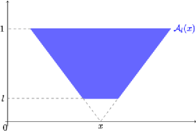
Figure 2: A graphical representation of the cone construction $\mathcal{A}_{l}(x)$.

(see Figure 2). The covariance kernel of the stationary Gaussian process $\omega_{l}$ is given by

$$K_{l}(x)=\cases{0,&\quad if $|x|\geq 1$,\vspace*{2pt}\cr\displaystyle\ln\frac{1}{|x|}+|x|-1,&\quad if $l\leq|x|\leq 1$,\vspace*{5pt}\cr\displaystyle\ln\frac{1}{l}+|x|-\frac{|x|}{l},&\quad if $|r|\leq l$,}$$ (47)

which can also be rewritten as

$$K_{l}(x)=\int_{1}^{1/l}\frac{(1-|xu|)_{+}}{u}\,du.$$

Therefore, the process $\omega_{e^{-t}}$ has the same law as $X_{t}$. This approach is called the cone construction.

Now we explain how to use the cone construction to prove Lemma 20, that, is to decompose the process $X_{s\ln 2}=\omega_{2^{-s}}$ for $s\in[n,n+1]$. So we choose $i\in\mathbb{N}$ such that $0\leq i\leq 2^{n}-1$. We call $\mathcal{A}_{i,n}$ the common part to all the cone like subsets $\mathcal{A}_{2^{-s}}(x)$ for $s\in[n,n+1]$ (see Figure 3) and $x\in I_{i,n}$,

$$\mathcal{A}_{i,n} = \bigcap_{s\in[n,n+1]}\bigcap_{x\in I_{i,n}}\mathcal{A}_{2^{-s}}(x)$$

$$= \biggl{\{}(u,y)\in\mathbb{R}\times\mathbb{R}^{*}_{+}\dvtx 2^{-n}\leq y\leq 1,-\frac{y}{2}+\frac{i+1}{2^{n}}\leq u\leq\frac{y}{2}+\frac{i}{2^{n}}\biggr{\}}.$$

For $s\in[n,n+1]$ and $x\in I_{i,n}$, we define the set $\mathcal{R}^{i,n}_{s}(x)$ as

$$\mathcal{R}^{i,n}_{s}(x)=\mathcal{A}_{2^{-s}}(x)\setminus\mathcal{A}_{i,n}.$$

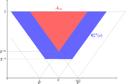
Figure 3: A graphical representation of $\mathcal{A}_{i,n}$.

Then we set $Y_{s}^{i,n}(x)=\mu(\mathcal{R}^{i,n}_{s}(x))$ and $X_{i,n}=\mu(\mathcal{A}_{i,n})$. In particular, we find

$$E[X_{i,n}X_{j,n}]=n\ln 2+\ln\frac{1}{|i-j|+1}+\frac{|i-j|+1}{2^{n}}-1.$$

It is then straightforward to check the claims of Lemma 20 by using the properties of the measure $\mu$. The process $(Y^{i,n}(x))_{s\in[n,n+1],x\in I_{i,n}}$ is independent of $X_{i,n}$ since the sets $(\mathcal{R}^{i,n}_{s}(x))_{s\in[n,n+1],x\in I_{i,n}}$ are all disjoint of the triangle $\mathcal{A}_{i,n}$. We also have

$$E\bigl{[}Y^{i,n}(x)Y^{j,n}\bigl{(}x^{\prime}\bigr{)}\bigr{]}\geq 0$$

since this covariance is just given by the $\Gamma$-measure of the set $\mathcal{R}^{i,n}_{s}(x)\cap\mathcal{R}^{i,n}_{s}(x^{\prime})$. The same argument holds to prove $E[Y^{i,n}(x)X_{j,n}]\geq 0$.

References

- (1) {barticle}[auto:STB—2014/01/06—10:16:28] \bauthor\bsnmAïdékon, \bfnmE.\binitsE. (\byear2013). \btitleConvergence in law of the minimum of a branching random walk. \bjournalAnn. Probab. \bvolume41 \bpages1362–1426. \bptokimsref\endbibitem
- (2) {bmisc}[auto:STB—2014/01/06—10:16:28] \bauthor\bsnmAïdékon, \bfnmE.\binitsE. and \bauthor\bsnmShi, \bfnmZ.\binitsZ. \bhowpublishedThe Seneta–Heyde scaling for the branching random walk. Available at \arxivurlarXiv:1102.0217v2. \bptokimsref\endbibitem
- (3) {barticle}[mr] \bauthor\bsnmAllez, \bfnmRomain\binitsR., \bauthor\bsnmRhodes, \bfnmRémi\binitsR. and \bauthor\bsnmVargas, \bfnmVincent\binitsV. (\byear2013). \btitleLognormal -scale invariant random measures. \bjournalProbab. Theory Related Fields \bvolume155 \bpages751–788. \biddoi=10.1007/s00440-012-0412-9, issn=0178-8051, mr=3034792 \bptnotecheck year \bptokimsref\endbibitem
- (4) {barticle}[mr] \bauthor\bsnmAlvarez-Gaumé, \bfnmL.\binitsL., \bauthor\bsnmBarbón, \bfnmJ. L. F.\binitsJ. L. F. and \bauthor\bsnmCrnković, \bfnmČ.\binitsČ. (\byear1993). \btitleA proposal for strings at . \bjournalNuclear Phys. B \bvolume394 \bpages383–422. \biddoi=10.1016/0550-3213(93)90020-P, issn=0550-3213, mr=1214333 \bptokimsref\endbibitem
- (5) {barticle}[mr] \bauthor\bsnmAmbjørn, \bfnmJ.\binitsJ., \bauthor\bsnmDurhuus, \bfnmB.\binitsB. and \bauthor\bsnmJónsson, \bfnmT.\binitsT. (\byear1994). \btitleA solvable D gravity model with . \bjournalModern Phys. Lett. A \bvolume9 \bpages1221–1228. \biddoi=10.1142/S0217732394001040, issn=0217-7323, mr=1279108 \bptokimsref\endbibitem
- (6) {barticle}[auto:STB—2014/01/06—10:16:28] \bauthor\bsnmArguin, \bfnmL.-P.\binitsL.-P. and \bauthor\bsnmZindy, \bfnmO.\binitsO. (\byear2014). \btitlePoisson–Dirichlet statistics for the extremes of a log-correlated Gaussian field. \bjournalAnn. Appl. Probab. \bvolume24 \bpages1446–1481. \bptokimsref\endbibitem
- (7) {barticle}[mr] \bauthor\bsnmBacry, \bfnmE.\binitsE. and \bauthor\bsnmMuzy, \bfnmJ. F.\binitsJ. F. (\byear2003). \btitleLog-infinitely divisible multifractal processes. \bjournalComm. Math. Phys. \bvolume236 \bpages449–475. \biddoi=10.1007/s00220-003-0827-3, issn=0010-3616, mr=2021198 \bptokimsref\endbibitem
- (8) {barticle}[mr] \bauthor\bsnmBarral, \bfnmJulien\binitsJ. (\byear1999). \btitleMoments, continuité, et analyse multifractale des martingales de Mandelbrot. \bjournalProbab. Theory Related Fields \bvolume113 \bpages535–569. \biddoi=10.1007/s004400050217, issn=0178-8051, mr=1717530 \bptokimsref\endbibitem
- (9) {barticle}[mr] \bauthor\bsnmBarral, \bfnmJulien\binitsJ., \bauthor\bsnmJin, \bfnmXiong\binitsX., \bauthor\bsnmRhodes, \bfnmRémi\binitsR. and \bauthor\bsnmVargas, \bfnmVincent\binitsV. (\byear2013). \btitleGaussian multiplicative chaos and KPZ duality. \bjournalComm. Math. Phys. \bvolume323 \bpages451–485. \biddoi=10.1007/s00220-013-1769-z, issn=0010-3616, mr=3096527 \bptnotecheck year \bptokimsref\endbibitem
- (10) {barticle}[mr] \bauthor\bsnmBarral, \bfnmJulien\binitsJ., \bauthor\bsnmKupiainen, \bfnmAntti\binitsA., \bauthor\bsnmNikula, \bfnmMiika\binitsM., \bauthor\bsnmSaksman, \bfnmEero\binitsE. and \bauthor\bsnmWebb, \bfnmChristian\binitsC. (\byear2014). \btitleCritical Mandelbrot cascades. \bjournalComm. Math. Phys. \bvolume325 \bpages685–711. \biddoi=10.1007/s00220-013-1829-4, issn=0010-3616, mr=3148099 \bptnotecheck year \bptokimsref\endbibitem
- (11) {barticle}[mr] \bauthor\bsnmBarral, \bfnmJulien\binitsJ. and \bauthor\bsnmMandelbrot, \bfnmBenoît B.\binitsB. B. (\byear2002). \btitleMultifractal products of cylindrical pulses. \bjournalProbab. Theory Related Fields \bvolume124 \bpages409–430. \biddoi=10.1007/s004400200220, issn=0178-8051, mr=1939653 \bptokimsref\endbibitem
- (12) {barticle}[mr] \bauthor\bsnmBarral, \bfnmJulien\binitsJ., \bauthor\bsnmRhodes, \bfnmRémi\binitsR. and \bauthor\bsnmVargas, \bfnmVincent\binitsV. (\byear2012). \btitleLimiting laws of supercritical branching random walks. \bjournalC. R. Math. Acad. Sci. Paris \bvolume350 \bpages535–538. \biddoi=10.1016/j.crma.2012.05.013, issn=1631-073X, mr=2929063 \bptnotecheck year \bptokimsref\endbibitem
- (13) {barticle}[mr] \bauthor\bsnmBenjamini, \bfnmItai\binitsI. and \bauthor\bsnmSchramm, \bfnmOded\binitsO. (\byear2009). \btitleKPZ in one dimensional random geometry of multiplicative cascades. \bjournalComm. Math. Phys. \bvolume289 \bpages653–662. \biddoi=10.1007/s00220-009-0752-1, issn=0010-3616, mr=2506765 \bptokimsref\endbibitem
- (14) {barticle}[mr] \bauthor\bsnmBernardi, \bfnmOlivier\binitsO. and \bauthor\bsnmBousquet-Mélou, \bfnmMireille\binitsM. (\byear2011). \btitleCounting colored planar maps: Algebraicity results. \bjournalJ. Combin. Theory Ser. B \bvolume101 \bpages315–377. \biddoi=10.1016/j.jctb.2011.02.003, issn=0095-8956, mr=2802884 \bptnotecheck year \bptokimsref\endbibitem
- (15) {barticle}[mr] \bauthor\bsnmBiggins, \bfnmJ. D.\binitsJ. D. and \bauthor\bsnmKyprianou, \bfnmA. E.\binitsA. E. (\byear2004). \btitleMeasure change in multitype branching. \bjournalAdv. in Appl. Probab. \bvolume36 \bpages544–581. \biddoi=10.1239/aap/1086957585, issn=0001-8678, mr=2058149 \bptokimsref\endbibitem
- (16) {barticle}[mr] \bauthor\bsnmBiggins, \bfnmJ. D.\binitsJ. D. and \bauthor\bsnmKyprianou, \bfnmA. E.\binitsA. E. (\byear2005). \btitleFixed points of the smoothing transform: The boundary case. \bjournalElectron. J. Probab. \bvolume10 \bpages609–631. \biddoi=10.1214/EJP.v10-255, issn=1083-6489, mr=2147319 \bptokimsref\endbibitem
- (17) {barticle}[mr] \bauthor\bsnmBramson, \bfnmMaury\binitsM. and \bauthor\bsnmZeitouni, \bfnmOfer\binitsO. (\byear2012). \btitleTightness of the recentered maximum of the two-dimensional discrete Gaussian free field. \bjournalComm. Pure Appl. Math. \bvolume65 \bpages1–20. \biddoi=10.1002/cpa.20390, issn=0010-3640, mr=2846636 \bptnotecheck year \bptokimsref\endbibitem
- (18) {barticle}[mr] \bauthor\bsnmBrézin, \bfnmÉ.\binitsÉ., \bauthor\bsnmKazakov, \bfnmV. A.\binitsV. A. and \bauthor\bsnmZamolodchikov, \bfnmAl. B.\binitsAl. B. (\byear1990). \btitleScaling violation in a field theory of closed strings in one physical dimension. \bjournalNuclear Phys. B \bvolume338 \bpages673–688. \biddoi=10.1016/0550-3213(90)90647-V, issn=0550-3213, mr=1063592 \bptokimsref\endbibitem
- (19) {barticle}[auto:STB—2014/01/06—10:16:28] \bauthor\bsnmCarpentier, \bfnmD.\binitsD. and \bauthor\bparticleLe \bsnmDoussal, \bfnmP.\binitsP. (\byear2001). \btitleGlass transition of a particle in a random potential, front selection in nonlinear RG and entropic phenomena in Liouville and Sinh–Gordon models. \bjournalPhys. Rev. E (3) \bvolume63 \bpages026110. \bptokimsref\endbibitem
- (20) {bbook}[auto:STB—2014/01/06—10:16:28] \bauthor\bsnmDaley, \bfnmD. J.\binitsD. J. and \bauthor\bsnmVere-Jones, \bfnmD.\binitsD. (\byear2007). \btitleAn Introduction to the Theory of Point Processes. Volume 2: Probability and Its Applications, \bedition2nd ed. \bpublisherSpringer, \blocationNew York. \bptokimsref\endbibitem
- (21) {barticle}[mr] \bauthor\bsnmDas, \bfnmSumit R.\binitsS. R., \bauthor\bsnmDhar, \bfnmAvinash\binitsA., \bauthor\bsnmSengupta, \bfnmAnirvan M.\binitsA. M. and \bauthor\bsnmWadia, \bfnmSpenta R.\binitsS. R. (\byear1990). \btitleNew critical behavior in large- matrix models. \bjournalModern Phys. Lett. A \bvolume5 \bpages1041–1056. \biddoi=10.1142/S0217732390001165, issn=0217-7323, mr=1057913 \bptokimsref\endbibitem
- (22) {bmisc}[auto:STB—2014/01/06—10:16:28] \bauthor\bsnmDaul, \bfnmJ.-M.\binitsJ.-M. \bhowpublished-state Potts model on a random planar lattice. Available at \arxivurlarXiv:hep-th/9502014. \bptokimsref\endbibitem
- (23) {barticle}[mr] \bauthor\bsnmDavid, \bfnmF.\binitsF. (\byear1988). \btitleConformal field theories coupled to -D gravity in the conformal gauge. \bjournalModern Phys. Lett. A \bvolume3 \bpages1651–1656. \biddoi=10.1142/S0217732388001975, issn=0217-7323, mr=0981529 \bptokimsref\endbibitem
- (24) {bmisc}[auto:STB—2014/01/06—10:16:28] \bauthor\bsnmDing, \bfnmJ.\binitsJ. and \bauthor\bsnmZeitouni, \bfnmO.\binitsO. \bhowpublishedExtreme values for two-dimensional discrete Gaussian free field. Available at \arxivurlarXiv:1206.0346v1. \bptokimsref\endbibitem
- (25) {barticle}[mr] \bauthor\bsnmDistler, \bfnmJacques\binitsJ. and \bauthor\bsnmKawai, \bfnmHikaru\binitsH. (\byear1989). \btitleConformal field theory and -D quantum gravity. \bjournalNuclear Phys. B \bvolume321 \bpages509–527. \biddoi=10.1016/0550-3213(89)90354-4, issn=0550-3213, mr=1005268 \bptokimsref\endbibitem
- (26) {barticle}[mr] \bauthor\bparticleDi \bsnmFrancesco, \bfnmP.\binitsP., \bauthor\bsnmGinsparg, \bfnmP.\binitsP. and \bauthor\bsnmZinn-Justin, \bfnmJ.\binitsJ. (\byear1995). \btitleD gravity and random matrices. \bjournalPhys. Rep. \bvolume254 \bpages1–133. \biddoi=10.1016/0370-1573(94)00084-G, issn=0370-1573, mr=1320471 \bptokimsref\endbibitem
- (27) {bincollection}[mr] \bauthor\bsnmDuplantier, \bfnmBertrand\binitsB. (\byear2004). \btitleConformal fractal geometry and boundary quantum gravity. In \bbooktitleFractal Geometry and Applications: A Jubilee of BenoîT Mandelbrot, Part 2. \bseriesProc. Sympos. Pure Math. \bvolume72 \bpages365–482. \bpublisherAmer. Math. Soc., \blocationProvidence, RI. \bidmr=2112128 \bptokimsref\endbibitem
- (28) {bincollection}[auto:STB—2014/01/06—10:16:28] \bauthor\bsnmDuplantier, \bfnmB.\binitsB. (\byear2010). \btitleA rigorous perspective on Liouville quantum gravity and KPZ. In \bbooktitleExact Methods in Low-Dimensional Statistical Physics and Quantum Computing (\beditor\bfnmJ.\binitsJ. \bsnmJacobsen, \beditor\bfnmS.\binitsS. \bsnmOuvry, \beditor\bfnmV.\binitsV. \bsnmPasquier, \beditor\bfnmD.\binitsD. \bsnmSerban and \beditor\bfnmL. F.\binitsL. F. \bsnmCugliandolo, eds.) \bpages529–561. \bpublisherOxford Univ. Press, \blocationOxford. \bidmr=2668656 \bptokimsref\endbibitem
- (29) {barticle}[mr] \bauthor\bsnmDuplantier, \bfnmBertrand\binitsB. and \bauthor\bsnmSheffield, \bfnmScott\binitsS. (\byear2009). \btitleDuality and the Knizhnik–Polyakov–Zamolodchikov relation in Liouville quantum gravity. \bjournalPhys. Rev. Lett. \bvolume102 \bpages150603. \biddoi=10.1103/PhysRevLett.102.150603, issn=0031-9007, mr=2501276 \bptokimsref\endbibitem
- (30) {barticle}[mr] \bauthor\bsnmDuplantier, \bfnmBertrand\binitsB. and \bauthor\bsnmSheffield, \bfnmScott\binitsS. (\byear2011). \btitleLiouville quantum gravity and KPZ. \bjournalInvent. Math. \bvolume185 \bpages333–393. \biddoi=10.1007/s00222-010-0308-1, issn=0020-9910, mr=2819163 \bptokimsref\endbibitem
- (31) {barticle}[pbm] \bauthor\bsnmDuplantier, \bfnmBertrand\binitsB. and \bauthor\bsnmSheffield, \bfnmScott\binitsS. (\byear2011). \btitleSchramm–Loewner evolution and Liouville quantum gravity. \bjournalPhys. Rev. Lett. \bvolume107 \bpages131305. \bidissn=1079-7114, pmid=22026841 \bptokimsref\endbibitem
- (32) {barticle}[mr] \bauthor\bsnmDurhuus, \bfnmB.\binitsB. (\byear1994). \btitleMulti-spin systems on a randomly triangulated surface. \bjournalNuclear Phys. B \bvolume426 \bpages203–222. \biddoi=10.1016/0550-3213(94)90132-5, issn=0550-3213, mr=1293688 \bptokimsref\endbibitem
- (33) {barticle}[mr] \bauthor\bsnmDurrett, \bfnmRichard\binitsR. and \bauthor\bsnmLiggett, \bfnmThomas M.\binitsT. M. (\byear1983). \btitleFixed points of the smoothing transformation. \bjournalProbab. Theory Related Fields \bvolume64 \bpages275–301. \biddoi=10.1007/BF00532962, issn=0044-3719, mr=0716487 \bptokimsref\endbibitem
- (34) {barticle}[mr] \bauthor\bsnmEynard, \bfnmB.\binitsB. and \bauthor\bsnmBonnet, \bfnmG.\binitsG. (\byear1999). \btitleThe Potts- random matrix model: Loop equations, critical exponents, and rational case. \bjournalPhys. Lett. B \bvolume463 \bpages273–279. \biddoi=10.1016/S0370-2693(99)00925-9, issn=0370-2693, mr=1722272 \bptokimsref\endbibitem
- (35) {barticle}[mr] \bauthor\bsnmFan, \bfnmAi Hua\binitsA. H. (\byear1997). \btitleSur les chaos de Lévy stables d’indice . \bjournalAnn. Sci. Math. Qué. \bvolume21 \bpages53–66. \bidissn=0707-9109, mr=1457064 \bptokimsref\endbibitem
- (36) {barticle}[mr] \bauthor\bsnmFyodorov, \bfnmYan V.\binitsY. V. and \bauthor\bsnmBouchaud, \bfnmJean-Philippe\binitsJ.-P. (\byear2008). \btitleFreezing and extreme-value statistics in a random energy model with logarithmically correlated potential. \bjournalJ. Phys. A \bvolume41 \bpages372001. \biddoi=10.1088/1751-8113/41/37/372001, issn=1751-8113, mr=2430565 \bptokimsref\endbibitem
- (37) {barticle}[auto:STB—2014/01/06—10:16:28] \bauthor\bsnmFyodorov, \bfnmY. V.\binitsY. V., \bauthor\bparticleLe \bsnmDoussal, \bfnmP.\binitsP. and \bauthor\bsnmRosso, \bfnmA.\binitsA. (\byear2009). \btitleStatistical mechanics of logarithmic REM: Duality, freezing and extreme value statistics of noises generated by Gaussian free fields \bjournalJ. Stat. Mech. \bpagesP10005. \bptokimsref\endbibitem
- (38) {bincollection}[auto:STB—2014/01/06—10:16:28] \bauthor\bsnmGinsparg, \bfnmP.\binitsP. and \bauthor\bsnmMoore, \bfnmG.\binitsG. (\byear1993). \btitleLectures on 2D gravity and 2D string theory. In \bbooktitleRecent Direction in Particle Theory (\beditor\bfnmJ.\binitsJ. \bsnmHarvey and \beditor\bfnmJ.\binitsJ. \bsnmPolchinski, eds.). \bpublisherWorld Scientific, \blocationSingapore. \bptokimsref\endbibitem
- (39) {barticle}[mr] \bauthor\bsnmGinsparg, \bfnmP.\binitsP. and \bauthor\bsnmZinn-Justin, \bfnmJ.\binitsJ. (\byear1990). \btitleD gravity D matter. \bjournalPhys. Lett. B \bvolume240 \bpages333–340. \biddoi=10.1016/0370-2693(90)91108-N, issn=0370-2693, mr=1053364 \bptokimsref\endbibitem
- (40) {barticle}[mr] \bauthor\bsnmGross, \bfnmDavid J.\binitsD. J. and \bauthor\bsnmKlebanov, \bfnmIgor\binitsI. (\byear1990). \btitleOne-dimensional string theory on a circle. \bjournalNuclear Phys. B \bvolume344 \bpages475–498. \biddoi=10.1016/0550-3213(90)90667-3, issn=0550-3213, mr=1076752 \bptokimsref\endbibitem
- (41) {barticle}[mr] \bauthor\bsnmGross, \bfnmDavid J.\binitsD. J. and \bauthor\bsnmMiljković, \bfnmNikola\binitsN. (\byear1990). \btitleA nonperturbative solution of string theory. \bjournalPhys. Lett. B \bvolume238 \bpages217–223. \biddoi=10.1016/0370-2693(90)91724-P, issn=0370-2693, mr=1050721 \bptokimsref\endbibitem
- (42) {barticle}[mr] \bauthor\bsnmGubser, \bfnmSteven S.\binitsS. S. and \bauthor\bsnmKlebanov, \bfnmIgor R.\binitsI. R. (\byear1994). \btitleA modified matrix model with new critical behavior. \bjournalPhys. Lett. B \bvolume340 \bpages35–42. \biddoi=10.1016/0370-2693(94)91294-7, issn=0370-2693, mr=1304657 \bptokimsref\endbibitem
- (43) {barticle}[mr] \bauthor\bsnmHu, \bfnmYueyun\binitsY. and \bauthor\bsnmShi, \bfnmZhan\binitsZ. (\byear2009). \btitleMinimal position and critical martingale convergence in branching random walks, and directed polymers on disordered trees. \bjournalAnn. Probab. \bvolume37 \bpages742–789. \biddoi=10.1214/08-AOP419, issn=0091-1798, mr=2510023 \bptokimsref\endbibitem
- (44) {barticle}[mr] \bauthor\bsnmJain, \bfnmSanjay\binitsS. and \bauthor\bsnmMathur, \bfnmSamir D.\binitsS. D. (\byear1992). \btitleWorld-sheet geometry and baby universes in D quantum gravity. \bjournalPhys. Lett. B \bvolume286 \bpages239–246. \biddoi=10.1016/0370-2693(92)91769-6, issn=0370-2693, mr=1175135 \bptokimsref\endbibitem
- (45) {barticle}[mr] \bauthor\bsnmKahane, \bfnmJean-Pierre\binitsJ.-P. (\byear1985). \btitleSur le chaos multiplicatif. \bjournalAnn. Sci. Math. Qué. \bvolume9 \bpages105–150. \bidissn=0707-9109, mr=0829798 \bptokimsref\endbibitem
- (46) {barticle}[mr] \bauthor\bsnmKahane, \bfnmJ.-P.\binitsJ.-P. and \bauthor\bsnmPeyrière, \bfnmJ.\binitsJ. (\byear1976). \btitleSur certaines martingales de Benoit Mandelbrot. \bjournalAdv. Math. \bvolume22 \bpages131–145. \bidissn=0001-8708, mr=0431355 \bptokimsref\endbibitem
- (47) {bincollection}[auto:STB—2014/01/06—10:16:28] \bauthor\bsnmKazakov, \bfnmV.\binitsV., \bauthor\bsnmKostov, \bfnmI.\binitsI. and \bauthor\bsnmKutasov, \bfnmD.\binitsD. (\byear2000). \btitleA matrix model for the 2d black hole. In \bbooktitleNonperturbative Quantum Effects. \bpublisherJHEP Proceedings. \bnoteAvailable at http://pos.sissa.it/cgi-bin/reader/conf.cgi?confid=6. \bptokimsref\endbibitem
- (48) {barticle}[mr] \bauthor\bsnmKlebanov, \bfnmIgor R.\binitsI. R. (\byear1995). \btitleTouching random surfaces and Liouville gravity. \bjournalPhys. Rev. D \bvolume51 \bpages1836–1841. \biddoi=10.1103/PhysRevD.51.1836, issn=0556-2821, mr=1320922 \bptokimsref\endbibitem
- (49) {barticle}[mr] \bauthor\bsnmKlebanov, \bfnmIgor R.\binitsI. R. and \bauthor\bsnmHashimoto, \bfnmAkikazu\binitsA. (\byear1995). \btitleNon-perturbative solution of matrix models modified by trace-squared terms. \bjournalNuclear Phys. B \bvolume434 \bpages264–282. \biddoi=10.1016/0550-3213(94)00518-J, issn=0550-3213, mr=1312995 \bptokimsref\endbibitem
- (50) {barticle}[mr] \bauthor\bsnmKlebanov, \bfnmIgor R.\binitsI. R. and \bauthor\bsnmHashimoto, \bfnmAkikazu\binitsA. (\byear1996). \btitleWormholes, matrix models, and Liouville gravity. \bjournalNuclear Phys. B Proc. Suppl. \bvolume45BC \bpages135–148. \bnoteString theory, gauge theory and quantum gravity (Trieste, 1995). \biddoi=10.1016/0920-5632(95)00631-1, issn=0920-5632, mr=1410550 \bptokimsref\endbibitem
- (51) {barticle}[mr] \bauthor\bsnmKnizhnik, \bfnmV. G.\binitsV. G., \bauthor\bsnmPolyakov, \bfnmA. M.\binitsA. M. and \bauthor\bsnmZamolodchikov, \bfnmA. B.\binitsA. B. (\byear1988). \btitleFractal structure of D-quantum gravity. \bjournalModern Phys. Lett. A \bvolume3 \bpages819–826. \biddoi=10.1142/S0217732388000982, issn=0217-7323, mr=0947880 \bptokimsref\endbibitem
- (52) {barticle}[mr] \bauthor\bsnmKostov, \bfnmI. K.\binitsI. K. (\byear1991). \btitleLoop amplitudes for nonrational string theories. \bjournalPhys. Lett. B \bvolume266 \bpages317–324. \biddoi=10.1016/0370-2693(91)91047-Y, issn=0370-2693, mr=1126824 \bptokimsref\endbibitem
- (53) {barticle}[mr] \bauthor\bsnmKostov, \bfnmIvan K.\binitsI. K. (\byear1992). \btitleStrings with discrete target space. \bjournalNuclear Phys. B \bvolume376 \bpages539–598. \biddoi=10.1016/0550-3213(92)90120-Z, issn=0550-3213, mr=1170955 \bptokimsref\endbibitem
- (54) {bincollection}[auto:STB—2014/01/06—10:16:28] \bauthor\bsnmKostov, \bfnmI. K.\binitsI. K. (\byear2010). \btitleBoundary loop models and 2D quantum gravity. In \bbooktitleExact Methods in Low-Dimensional Statistical Physics and Quantum Computing (\beditor\bfnmJ.\binitsJ. \bsnmJacobsen, \beditor\bfnmS.\binitsS. \bsnmOuvry, \beditor\bfnmV.\binitsV. \bsnmPasquier, \beditor\bfnmD.\binitsD. \bsnmSerban and \beditor\bfnmL. F.\binitsL. F. \bsnmCugliandolo, eds.) \bpages363–406. \bpublisherOxford Univ. Press, \blocationOxford. \bidmr=2668651 \bptokimsref\endbibitem
- (55) {barticle}[mr] \bauthor\bsnmKostov, \bfnmIvan K.\binitsI. K. and \bauthor\bsnmStaudacher, \bfnmMatthias\binitsM. (\byear1992). \btitleMulticritical phases of the model on a random lattice. \bjournalNuclear Phys. B \bvolume384 \bpages459–483. \biddoi=10.1016/0550-3213(92)90576-W, issn=0550-3213, mr=1188360 \bptokimsref\endbibitem
- (56) {barticle}[mr] \bauthor\bsnmKyprianou, \bfnmA. E.\binitsA. E. (\byear1998). \btitleSlow variation and uniqueness of solutions to the functional equation in the branching random walk. \bjournalJ. Appl. Probab. \bvolume35 \bpages795–801. \bidissn=0021-9002, mr=1671230 \bptokimsref\endbibitem
- (57) {barticle}[mr] \bauthor\bsnmLiu, \bfnmQuansheng\binitsQ. (\byear1998). \btitleFixed points of a generalized smoothing transformation and applications to the branching random walk. \bjournalAdv. in Appl. Probab. \bvolume30 \bpages85–112. \biddoi=10.1239/aap/1035227993, issn=0001-8678, mr=1618888 \bptokimsref\endbibitem
- (58) {bmisc}[auto:STB—2014/01/06—10:16:28] \bauthor\bsnmMadaule, \bfnmT.\binitsT. \bhowpublishedConvergence in law for the branching random walk seen from its tip. Available at \arxivurlarXiv:1107.2543v2. \bptokimsref\endbibitem
- (59) {bincollection}[auto:STB—2014/01/06—10:16:28] \bauthor\bsnmMandelbrot, \bfnmB. B.\binitsB. B. (\byear1972). \btitleA possible refinement of the lognormal hypothesis concerning the distribution of energy in intermittent turbulence. In \bbooktitleStatistical Models and Turbulence \bpages333–351. \bpublisherSpringer, \blocationNew York. \bptokimsref\endbibitem
- (60) {barticle}[mr] \bauthor\bsnmMotoo, \bfnmMinoru\binitsM. (\byear1958). \btitleProof of the law of iterated logarithm through diffusion equation. \bjournalAnn. Inst. Statist. Math. \bvolume10 \bpages21–28. \bidissn=0020-3157, mr=0097866 \bptnotecheck year \bptokimsref\endbibitem
- (61) {barticle}[mr] \bauthor\bsnmNakayama, \bfnmYu\binitsY. (\byear2004). \btitleLiouville field theory: A decade after the revolution. \bjournalInternat. J. Modern Phys. A \bvolume19 \bpages2771–2930. \biddoi=10.1142/S0217751X04019500, issn=0217-751X, mr=2073993 \bptokimsref\endbibitem
- (62) {bincollection}[mr] \bauthor\bsnmNeveu, \bfnmJ.\binitsJ. (\byear1988). \btitleMultiplicative martingales for spatial branching processes. In \bbooktitleSeminar on Stochastic Processes, 1987 (Princeton, NJ, 1987) (\beditor\bfnmE.\binitsE. \bsnmCinlar, \beditor\bfnmK. L.\binitsK. L. \bsnmChung and \beditor\bfnmR. K.\binitsR. K. \bsnmGetoor, eds.). \bseriesProgr. Probab. Statist. \bvolume15 \bpages223–241. \bpublisherBirkhäuser, \blocationBoston, MA. \bidmr=1046418 \bptokimsref\endbibitem
- (63) {bincollection}[mr] \bauthor\bsnmNienhuis, \bfnmB.\binitsB. (\byear1987). \btitleCoulomb gas formulation of two-dimensional phase transitions. In \bbooktitlePhase Transitions and Critical Phenomena (\beditor\bfnmC.\binitsC. \bsnmDomb and \beditor\bfnmJ. L.\binitsJ. L. \bsnmLebowitz, eds.). \bpublisherAcademic Press, \blocationLondon. \bidmr=0942673 \bptokimsref\endbibitem
- (64) {barticle}[mr] \bauthor\bsnmParisi, \bfnmGiorgio\binitsG. (\byear1990). \btitleOn the one-dimensional discretized string. \bjournalPhys. Lett. B \bvolume238 \bpages209–212. \biddoi=10.1016/0370-2693(90)91722-N, issn=0370-2693, mr=1050719 \bptokimsref\endbibitem
- (65) {barticle}[mr] \bauthor\bsnmPolchinski, \bfnmJoseph\binitsJ. (\byear1990). \btitleCritical behavior of random surfaces in one dimension. \bjournalNuclear Phys. B \bvolume346 \bpages253–263. \biddoi=10.1016/0550-3213(90)90280-Q, issn=0550-3213, mr=1080693 \bptokimsref\endbibitem
- (66) {barticle}[mr] \bauthor\bsnmRajput, \bfnmBalram S.\binitsB. S. and \bauthor\bsnmRosiński, \bfnmJan\binitsJ. (\byear1989). \btitleSpectral representations of infinitely divisible processes. \bjournalProbab. Theory Related Fields \bvolume82 \bpages451–487. \biddoi=10.1007/BF00339998, issn=0178-8051, mr=1001524 \bptokimsref\endbibitem
- (67) {barticle}[auto:STB—2014/01/06—10:16:28] \bauthor\bsnmRhodes, \bfnmR.\binitsR., \bauthor\bsnmSohier, \bfnmJ.\binitsJ. and \bauthor\bsnmVargas, \bfnmV.\binitsV. (\byear2014). \btitleLevy multiplicative chaos and star scale invariant random measures. \bjournalAnn. Probab. \bvolume42 \bpages689–724. \bptokimsref\endbibitem
- (68) {barticle}[mr] \bauthor\bsnmRhodes, \bfnmRémi\binitsR. and \bauthor\bsnmVargas, \bfnmVincent\binitsV. (\byear2010). \btitleMultidimensional multifractal random measures. \bjournalElectron. J. Probab. \bvolume15 \bpages241–258. \biddoi=10.1214/EJP.v15-746, issn=1083-6489, mr=2609587 \bptokimsref\endbibitem
- (69) {barticle}[mr] \bauthor\bsnmRhodes, \bfnmRémi\binitsR. and \bauthor\bsnmVargas, \bfnmVincent\binitsV. (\byear2011). \btitleKPZ formula for log-infinitely divisible multifractal random measures. \bjournalESAIM Probab. Stat. \bvolume15 \bpages358–371. \biddoi=10.1051/ps/2010007, issn=1292-8100, mr=2870520 \bptokimsref\endbibitem
- (70) {bmisc}[auto:STB—2014/01/06—10:16:28] \bauthor\bsnmSheffield, \bfnmS.\binitsS. \bhowpublishedConformal weldings of random surfaces: SLE and the quantum gravity zipper. Available at \arxivurlarXiv:1012.4797. \bptokimsref\endbibitem
- (71) {barticle}[mr] \bauthor\bsnmSheffield, \bfnmScott\binitsS. (\byear2007). \btitleGaussian free fields for mathematicians. \bjournalProbab. Theory Related Fields \bvolume139 \bpages521–541. \biddoi=10.1007/s00440-006-0050-1, issn=0178-8051, mr=2322706 \bptokimsref\endbibitem
- (72) {barticle}[mr] \bauthor\bsnmSugino, \bfnmFumihiko\binitsF. and \bauthor\bsnmTsuchiya, \bfnmOsamu\binitsO. (\byear1994). \btitleCritical behavior in matrix model with branching interactions. \bjournalModern Phys. Lett. A \bvolume9 \bpages3149–3162. \biddoi=10.1142/S0217732394002975, issn=0217-7323, mr=1306193 \bptokimsref\endbibitem
- (73) {bmisc}[auto:STB—2014/01/06—10:16:28] \bauthor\bsnmTecu, \bfnmN.\binitsN. \bhowpublishedRandom conformal welding at criticality. Available at \arxivurlarXiv:1205.3189v1. \bptokimsref\endbibitem