Synchronization of globally coupled two-state stochastic oscillators with a state-dependent refractory period

Abstract

We present a model of identical coupled two-state stochastic units each of which in isolation is governed by a fixed refractory period. The nonlinear coupling between units directly affects the refractory period, which now depends on the global state of the system and can therefore itself become time dependent. At weak coupling the array settles into a quiescent stationary state. Increasing coupling strength leads to a saddle node bifurcation, beyond which the quiescent state coexists with a stable limit cycle of nonlinear coherent oscillations. We explicitly determine the critical coupling constant for this transition.

I Introduction

Many dynamical processes in nature can in the first instance be modeled as on-off processes. Examples include firing of neurons ElsonPRL98 ; Murray , up-down spin systems, and blinking phenomena fran . Although the dynamics of such on-off single systems is simple, when coupled together in large numbers they are known to exhibit complex global dynamical behaviors such as synchronization, in which the entire system evolves as a single unit. The study of the synchronized dynamics of two-state networks is essential not only as a problem of fundamental scientific importance Zhou , but also as a tool to help us understand many physiological processes GlassNature2001 . For example, our cardiac system is a giant network of synchronized oscillators. A vast number of systems in physics and engineering also share such synchronization features Pikovsky ; StrogatzPRL96 .

Coupled two-state units offer the simplest example of coupled units of discrete states. Such discrete models are useful for the study of phase synchronization of stochastic coupled oscillators Wood ; Wood2 and of excitable media Prager ; Kouvaris . They can be invoked in ecological applications BerandIJBC2000 where populations of various species interlinked through the food chain exhibit spatial and temporal synchronization. For sufficiently weak coupling between oscillators, the system as a whole typically reaches a stationary state where on average the dynamics ceases to exist. However, for relatively strong coupling each unit is driven away from its equilibrium, and the system as a whole may undergo a transition to a non-stationary state.

Phase synchronization on networks has most commonly been analyzed in terms of a Hopf bifurcation Wood ; Wood2 ; Prager ; Kouvaris , that is, as a linear instability of the stationary state. Synchronization may also occur via other bifurcation mechanisms such as, for instance, saddle node or homoclinic bifurcations StrogatzLib . A sub-critical Hopf bifurcation may, for example, involve a prior saddle node which can not be captured within the linear analysis. Such sub-critical scenarios have been observed in a variety of different contexts including the Kuramoto model paso , Kuramoto model with time-delayed interactions Yeung , globally coupled noisy bistable elements also with time delayed interactions Huber , and three-state coupled oscillators Wood2 . These cases all involve the coexistence of a synchronous oscillatory state and a quiescent stationary state, with the corresponding hysteresis loop.

The novelty of our model lies in the occurence of synchrony without destabilization of the stationary state, so that the oscillatory state may coexist with it without exhibiting hysteresis. In this scenario transitions between the synchronous phase and the asynchronous phase can only be induced by a strong perturbation.

For a purely Markovian system the master equation is an ordinary differential equation. For coupled two-state systems it is a first order equation, which only has a fixed point. Therefore, in order to observe global synchronization in purely Markovian networks it is necessary to go beyond a two-state model Wood ; Wood2 . Converseley, to observe synchronization in a two-state system it is necessary to go beyond a simple Markovian model of coupled units. The synchronization of two-state units was perhaps first observed in the context of collective molecular motors, where spatial elastic coupling to a common environment leads to the occurrence of oscillations Julicher . In globally coupled networks of two-state units, memory effects can also lead to synchronization Kouvaris . In recent studies of coupled assemblies of genetic oscillators Tsimring , memory (delay) effects have been found to play a significant role in the description of the observed synchronous dynamics of the on and the off (active and inactive) states of the system.

Time delays in network dynamics can be introduced in many different ways. One is to introduce time delays in the interaction between the elements of the network Yeung ; Huber . Another is to include a refractory period in the internal dynamics of the units Prager . Both of these together have also been considered Kouvaris . Most of the models with a time delay that have been reported in the literature consider uniform fixed time delays, be it in the internal dynamics and/or in the interactions. Huber and Tsimring suggested that temporally nonuniform (that is, distributed) time delays do not qualitatively affect the synchronization features observed in their model Huber . A more detailed analysis of the role of nonuniform time delays in synchronization has been reported in a cellular automaton version of the susceptible-infected-recovered-susceptible model Rozenblit , where a probabilistic refractory period is studied.

In this work we also consider the effects of delay times, but of an altogether different kind than those described above. We consider identical two-state stochastic elements with a fixed refractory period. The units are then coupled together all to all. The interactions among the elements affect the internal dynamics in that the refractory period becomes dependent on the time-dependent state of the entire network. By combining numerical and analytical results, we find that a global dynamics may emerge as the coupling strength is increased beyond a critical value. We observe that synchronization occurs for some initial conditions but not for others. Unlike the usual case of a Hopf bifurcation, the synchronized behavior here emerges as a result of a saddle node bifurcation in the master equation phase space.

The paper is organized as follows: In Sec. II we introduce our general model and show that no Hopf bifurcation is possible for this type of dynamics. In Sec. III we choose a specific model and show via numerical results that a global synchronized dynamics exists for our model. We also check the robustness of our results by considering some variants of the model. By computing a Poincaré-type of map for the oscillatory state, in Sec. IV we demostrate that synchrony appears via a saddle node bifurcation, and compute the critical point using this map. We confirm the critical point by direct integration of the generalized master equation. We end with some concluding remarks in Sec. V.

II The General Model

II.1 The basic unit

Our starting point is a binary unit characterized by two states, $1$ and $2$. Transitions from state $1$ to state $2$ are governed by a Markovian (memoryless) process of rate $\gamma$, while transitions from $2$ back to $1$ occur after a fixed delay time $\tau$ measured from the time of the transition to $2$ (Fig. 1). The waiting time distribution $\psi_{1\to 2}(t)$ for a transition from $1$ to $2$ is thus an exponential, $\psi_{1\to 2}=\gamma e^{-\gamma t}$, while that of a transition from $2$ to $1$ is a $\delta$-function, $\psi_{2\to 1}=\delta(t-\tau)$.

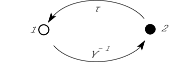
Figure 1: Isolated binary unit. Transitions from state $1$ to state $2$ occur at random times $\gamma^{-1}$ according to a Markov process of rate $\gamma$, while transitions from $2$ to $1$ occur at exactly time $\tau$ after arrival at $2$.

We next construct the generalized master equation for the probabilities $P_{i}(t)$ to be in state $i=1,2$ at time $t$. Normalization reduces this to a single probability, since $P_{1}(t)=1-P_{2}(t)$. Further, it is evident that

$$P_{2}(t)=\int_{t-\tau}^{t}dt^{\prime}J_{1\rightarrow 2}\left(t^{\prime}\right),$$ (1)

where $J_{1\rightarrow 2}\left(t^{\prime}\right)dt$ is the probability of jumping from state $1$ to state $2$ at some time within the interval $[t^{\prime},t^{\prime}+dt^{\prime}]$, with $t^{\prime}$ lying in the range $[t-\tau,t]$. (If $t^{\prime}$ were to lie below this range, the jump from state $2$ back to state $1$ would have occurred already before time $t$.) In turn, $J_{1\rightarrow 2}\left(t^{\prime}\right)dt^{\prime}=\gamma P_{1}(t^{\prime})dt^{\prime}$, the probability of being in state $1$ times the jumping rate to state $2$. It follows that

$$P_{2}(t)=\gamma\int_{t-\tau}^{t}dt^{\prime}\left[1-P_{2}(t^{\prime})\right].$$ (2)

This linear integral equation for $P_{2}$ can also be written in differential form to arrive at the master equation

$$\mathcal{L}P_{2}=\gamma\tau,$$ (3)

where the linear operator $\mathcal{L}$ involves infinite derivatives,

$$\mathcal{L}=1+\gamma\tau\sum_{n=0}^{\infty}\frac{\left(-\tau\right)^{n}}{\left(n+1\right)!}\left(\frac{d}{dt}\right)^{n}.$$ (4)

The master equation (3) predicts that, after a transient, the system reaches a stationary equilibrium, $P_{2}(t)\rightarrow P_{2}^{*}$, which is determined by the rate $\gamma$ and the refractory period $\tau$ via the equation

$$P_{2}^{*}=\frac{\gamma\tau}{1+\gamma\tau}.$$ (5)

This result is easily understood: at equilibrium, the mean time spent by the unit in state $1$ is $\bar{\tau}_{1}=\gamma^{-1}$, while the mean time spent in state $2$ is exactly the refractory period, $\bar{\tau}_{2}=\tau$. The equilibrium probability $P_{2}^{*}$ is then simply the fraction of the time spent in state $2$,

$$P_{2}^{*}=\frac{\bar{\tau}_{2}}{\bar{\tau}_{1}+\bar{\tau}_{2}},$$ (6)

which immediately leads to Eq. (5).

We can furthermore see, as follows, that the equilibrium probability $P_{2}^{*}$ is always the single stable solution. Equation (2) is linear and invariant under time translation. We can therefore pick any time $t_{0}$ and we know that if a unit is in state $2$, it must have transitioned there at some time during the time interval $(t_{0}-\tau,t_{0})$. Had it transitioned to state $2$ earlier than that, say in the interval $(t_{0}-2\tau,t_{0}-\tau)$, it would have returned to state $1$ before time $t_{0}$. If it transitioned to $2$ before time $t_{0}-2\tau$, it might return and be back in state $2$ at time $t_{0}$, but this event is already accounted for in the accounting of transitions in the interval $(t_{0}-\tau,t_{0})$. One can thus write the transient solution as

$$P_{2}(t)=P_{2}^{*}+\sum_{n=1}^{\infty}q_{n}e^{\lambda_{n}t},$$ (7)

where the set $\left\{q_{n}\right\}_{n=1}^{\infty}$ depends on the “initial condition,” that is, on the function $P_{2}(t)$ in the time interval $[t_{0}-\tau,t_{0}]$, and $\left\{\lambda_{n}\right\}_{n=1}^{\infty}$ is the set of solutions of the equation

$$\frac{e^{-\lambda_{n}\tau}-1}{\lambda_{n}}=\gamma^{-1}.$$ (8)

The real and imaginary parts separately, $\lambda_{n}=\rho_{n}+i\omega_{n}$, obey the equations

$$e^{-\rho_{n}\tau}\cos\left(\omega_{n}\tau\right)-1=\gamma^{-1}\rho_{n},$$

$$e^{-\rho_{n}\tau}\sin\left(\omega_{n}\tau\right)=-\gamma^{-1}\omega_{n}.$$ (9)

From Eq. (8) it is clear that the solution $\rho_{n}=\omega_{n}=0$ is spurious. Furthermore, the choice $\rho_{n}>0$ leads to an immediate contradiction, namely, that $\gamma<0$. This is impossible since $\gamma$ is a rate, hence positive. Therefore the real parts of the $\lambda_{n}$ must all be negative, and thus $P_{2}(t)$ goes to $P_{2}^{*}$ for any initial condition. Indeed, the dynamics of an ensemble of $N$ such isolated units consists of a transient of damped oscillations and eventual arrival at equilibrium, with fluctuations due to the finite number of units. A typical evolution of $N$ such independent units is shown in Fig. 2, where we show $P_{2}(t)=N_{2}(t)/N$ vs $t$. Here $N_{2}(t)$ is the number of units in state $2$. The small fluctuations just visible in the figure can be further mitigated by working with a larger number of units.

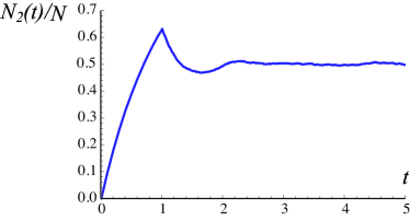
Figure 2: Ensemble of $N=2\times 10^{4}$ isolated units with $\gamma=1$ and $\tau=1$, which leads to $P_{2}^{*}=1/2$.

II.2 Coupled array: Generalized master equation

Next we globally couple $N$ of these two-state oscillators, that is, each oscillator is coupled to all the other oscillators. We point with special emphasis to the nature of the coupling about to be described, because it is this feature that distinguishes our model from others in the literature.

We take the transition rate from state $1$ to state $2$, and the refractory period in state $2$ to become functions of the global state of the system. These are therefore themselves now time dependent. That is, if at a time $t$ there are $N_{1}$ units in state $1$ and $N_{2}$ units in state $2$ (always with the constraint $N=N_{1}+N_{2}$), the time-dependent transition rate and refractory period are modified from their values in the isolated units,

$$\gamma \rightarrow \gamma(t)=\gamma\left(\frac{N_{2}(t)}{N}\right)\rightarrow\gamma(P_{2}(t)),$$ (10a)

$$\tau \rightarrow \tau(t)=\tau\left(\frac{N_{2}(t)}{N}\right)\rightarrow\tau(P_{2}(t)).$$ (10b)

Here we have indicated the implementation of the thermodynamic limit $N\to\infty$,

$$\frac{N_{2}(t)}{N}\rightarrow P_{2}(t),$$ (11)

and we recall again that $P_{1}(t)=1-P_{2}(t)$. We have not yet specified the explicit form of the dependences on the state, but only that the transition rate from $1$ to $2$ and the transition delay from $2$ back to $1$ are now functions of the state. Recall that in the single units, an oscillator that arrived at state $2$ at time $t-\tau$ jumped back to state $1$ at time $t$. In an uncoupled collection of single units, the times at which different units are observed to leave state $2$ are random because the arrival times are random. However, the length of time spent in state $2$ after each arrival is fixed at the value $\tau$. In a coupled array once again units arrive at state $2$ at random times but remain there for a fixed time period. Because of the random arrival, the departures are also randomly distributed. However, there are now two differences. The rate at which units leave state $1$ is not fixed but depends on the instantaneous state of the coupled system. Similarly, the waiting time in state $2$ varies with system state. We clarify what we mean by the time dependence of the refractory period, without yet fixing the form of the dependence implicit in Eq. (10b): all the oscillators that arrived at state $2$ at time $t-\tau(t)$ jump back to state $1$ at time $t$. Thus if one has a number of units in state $2$ at time $t$, some will jump back to state $1$ right then and some not, depending on their arrival time. We emphasize that this is not a stochastic feature of $\tau(t)$ but rather a consequence of the stochasticity in the arrival times embodied in $\gamma(t)$.

To accommodate these time dependences in a mean field description appropriate for all-to-all coupling, we generalize the master equation (2),

$$P_{2}(t)=\int_{-\infty}^{t}dt^{\prime}F\left(P_{2}(t^{\prime})\right)\Theta(t,t^{\prime}).$$ (12)

Here

$$F\left(P_{2}(t^{\prime})\right)dt^{\prime}=\gamma\left(P_{2}(t^{\prime})\right)\left[1-P_{2}(t^{\prime})\right]dt^{\prime}$$ (13)

is the probability to jump from state $1$ to state $2$ at some time within the interval $[t^{\prime},t^{\prime}+dt^{\prime}]$; the factor $1-P_{2}(t^{\prime})=P_{1}(t^{\prime})$ is the probability to be in state $1$ at time $t^{\prime}$, and $\gamma\left(P_{2}(t^{\prime})\right)$ is the (ever-changing) rate at which the jump from $1$ to $2$ takes place at time $t^{\prime}$. The factor $\Theta(t,t^{\prime})$ keeps track of this arrival rate and “freezes” each oscillator in state 2 for a precise length of time (refractory period) determined by the state of the system when the oscillator arrived there.

We have highlighted this last term because the core and novelty of our model lie in it. Consider the units that arrive at state $2$ at time $t^{\prime}$. The number of arrivals is stochastic since the departure from state $1$ is random. Furthermore, the rate of random arrivals depends on the state of the system at that time, $\gamma\left(P_{2}(t^{\prime})\right)$. The departure of these units from state $2$ occurs at a definite delay time $t^{\prime\prime}$ later, $t^{\prime\prime}-t^{\prime}=\tau(t^{\prime\prime})$, which depends on the state $P_{2}(t^{\prime\prime})$ at the time of departure. If $t^{\prime\prime}-t^{\prime}<\tau(t^{\prime\prime})$ we know that the units that arrived at $t^{\prime}$ have not departed. On the other hand, if $t^{\prime\prime}-t^{\prime}>\tau(t^{\prime\prime})$ we know that they have. Thus, if the delay time $\tau(t^{\prime\prime})$ is not reached at any time $t^{\prime\prime}$ in the interval $[t^{\prime},t]$, we have that $\Theta\left(t,t^{\prime}\right)=1$, an indication that all the oscillators that arrived in state $2$ at time $t^{\prime}$ are still there (while others may continue to arrive). If the delay time is reached at any time within the interval, then $\Theta(t,t^{\prime})=0$ because the units that arrived in state $2$ at time $t^{\prime}$ have left again. This step-like function character arises from the fact that the delay time is fixed by the population probabilities, that is, it is not a random variable. Explicitly, $\Theta$ is the step-like function

$$\Theta(t,t^{\prime})=\left\{\begin{array}[c]{ll}1&\text{if }\forall t^{\prime\prime}\in\left[t^{\prime},t\right]\text{, }t^{\prime\prime}-t^{\prime}<\tau\left[P_{2}\left(t^{\prime\prime}\right)\right]\\ 0&\text{otherwise}\\ \end{array}\right..$$ (14)

We call the condition that leads to $\Theta(t,t^{\prime})=1$ the inequality. In Appendix A we explore this question in detail independently of the particular functional form of $\gamma$ and $\tau$ as functions of time. Here we take advantage of the lessons learned there and implement the behaviors that arise in our case.

Our ultimate goal is to find the behavior of the $P_{i}(t)$ at long times. In particular, we are interested in establishing whether this behavior is time dependent or time independent, and under what conditions one might observe the former or the latter.

II.3 Stationary solutions

We start by exploring the possible occurrence of one or more stationary states, that is, one or more time-independent solutions $P_{2}(t)=P_{2}^{*}$. This case is covered by the first part of Appendix A and falls in the class of behaviors described by the generalized master equation (39),

$$P_{2}(t)=\int_{t-\tau(P_{2}(t))}^{t}dt^{\prime}F\left(P_{2}(t^{\prime})\right).$$ (15)

Specifically, such a stationary solution would satisfy

$$P_{2}^{*}=\frac{\gamma\left(P_{2}^{*}\right)\tau\left(P_{2}^{*}\right)}{1+\gamma\left(P_{2}^{*}\right)\tau\left(P_{2}^{*}\right)}.$$ (16)

Note that this is only similar to Eq. (5) for the uncoupled system in aspect since Eq. (16) is in general a non-linear equation for quiescent states. This nonlinear equation could have more than one solution (multi-stability) or even no solution at all, depending on the particular functional forms chosen for $\gamma\left(P_{2}\right)$ and $\tau\left(P_{2}\right)$.

II.4 Absence of Hopf-type instabilities

While we have not yet established whether Eq. (16) actually has one or more solutions, we can show that the coupled array does not support Hopf-type instabilities leading to oscillatory or chaotic solutions. Indeed, a linear analysis at best leads to other quiescent solutions. To show this we introduce a perturbation,

$$P_{2}(t)=P_{2}^{*}+\varepsilon e^{\mu t},$$ (17)

with $\left|\varepsilon\right|\ll 1$. First, we note that if $\tau^{\prime}(P_{2}(t))\sim\mathcal{O}(1)$, as it will be in our model explicitly introduced later, then $d\tau\left(P_{2}(t)\right)/dt\sim\varepsilon<1$. (The prime denotes a derivative with respect to the argument.) According to the discussion in the appendix, the generalized master equation (15) is valid if $\mu$ is negative and for sufficiently short times even if $\mu$ is positive. To first order in $\varepsilon$, the master equation is then given by

$$\varepsilon e^{\mu t}= \varepsilon\int_{t-\tau\left(P_{2}^{*}\right)}^{t}dt^{\prime}F^{\prime}\left(P_{2}^{*}\right)e^{\mu t^{\prime}}$$

$$+\int_{t-\tau\left(P_{2}^{*}\right)-\varepsilon\tau^{\prime}\left(P_{2}^{*}\right)e^{\mu t}}^{t-\tau\left(P_{2}^{*}\right)}dt^{\prime}F\left(P_{2}^{*}\right).$$

Straight substitution of Eq. (16) in this equation shows that $\mu$ must satisfy

$$\frac{e^{-\mu\tau^{*}}-1}{\mu}=\Gamma^{-1},$$ (18)

where

$$\tau^{*}\equiv\tau\left(P_{2}^{*}\right),\qquad\Gamma=\frac{F^{\prime}\left(P_{2}^{*}\right)}{\tau^{\prime}\left(P_{2}^{*}\right)F\left(P_{2}^{*}\right)-1}.$$

Therefore, all the information about the linear stability of $P_{2}^{*}$ resides in the two numbers $\tau^{*}$ and $\Gamma$. No additional information about the specific functional form of $\tau(P_{2})$ or of $\gamma(P_{2})$ is required.

To analyze equation (18) one can separate the real and imaginary parts, $\mu=\beta+i\Omega,$ in terms of which condition (18) can be separated into the two equations

$$1-e^{-\beta\tau^{*}}\cos\left(\Omega\tau^{*}\right) =\Gamma^{-1}\beta,$$

$$e^{-\beta\tau^{*}}\sin\left(\Omega\tau^{*}\right) =\Gamma^{-1}\Omega.$$

A Hopf-type instability requires that a stable stationary solution become unstable with non-zero frequency. A critical point must satisfy $\beta_{c}=0\text{ with }\Omega_{c}\neq 0,$ that is,

$$\cos\left(\Omega_{c}\tau^{*}\right)=1\text{ and }\sin\left(\Omega_{c}\tau^{*}\right)=\Gamma^{-1}\Omega_{c}.$$

However, this pair of equations only has the solution $\Omega_{c}=0$. Note that the solution $\mu=0$ is no longer necessarily spurious as it was in the decoupled array. There the solution $\lambda_{n}=0$ required that $\gamma\tau=-1$ [cf. Eq. (8)], which is impossible because both parameters are positive. However, here the condition $\Gamma\tau^{*}=-1$ can be seen as an equation for a critical value of the control parameter.

In summary, this linear analysis predicts no complexity beyond possible bifurcations between stationary solutions. However, the analysis itself is limited: our nonlinear infinite-dimensional system has the potential to exhibit more complex behavior such as oscillatory or chaotic orbits. We will next explore the possible occurrence of limit cycles (synchronization of the units) via global bifurcations, that is, bifurcations that go beyond the vicinity of a fixed point to involve larger regions of phase space. For low dimensional systems there are three generic global bifurcation pathways to cycles StrogatzLib : saddle-node, infinite-period and homoclinic bifurcations. We find below that our infitine-dimensional system also follows one of these pathways.

II.5 Generic features beyond stationary states

We continue to explore possible behaviors, now away from stationary states. Our analysis in Appendix A shows that there is only a limited array of possible behaviors. We will basically encounter only two.

The first, which we will call behavior $B$, occurs when $\Theta(t,t^{\prime})$ can be expressed as a Heaviside function, cf. Eq. (38) in the appendix,

$$\Theta(t,t^{\prime})=\theta\left(t^{\prime}-t+\tau(P_{2}(t))\right).$$ (19)

As shown in the appendix, this expression is valid when (1) $\tau(t)$ is continuous and piecewise differentiable; (2) where differentiable, $d\tau/dt<1$; (3) $\tau(t)$ may have discontinuities presenting a downward jump from a high value to a low value as time increases, but not from a low value to a high value.

The other behavior we will encounter, behavior A, occurs in one of two ways. It can come about because (3) above is violated, that is, $\tau(t)$ exhibits a discontinuity presenting an upward jump from a low value to a high value, or because condition (2) above is violated. There are several ways to violate the condition $d\tau/dt<1$ and thus to enter regime A. These four ways are illustrated in Fig. 3. One, illustrated in the upper right panel of the figure, occurs smoothly. It starts at time $t_{1}$ where $d\tau/dt|_{t=t_{1}}=1$. A second way to enter regime A is illustrated in the lower left panel. Here regime A again begins at time $t_{1}$, but $\tau(t)$ need not be differentiable at $t_{1}$. Instead, here $\lim_{t\to t_{1}^{+}}(d\tau/dt)>1$. The third way to enter regime A, illustrated in the lower right panel, is via a discontinuity from a high value to a low value at time $t_{1}$, but with a violation of condition (2) above, that is, again $\lim_{t\to t_{1}^{+}}(d\tau/dt)>1$. The final way, illustrated in the upper left panel, occurs when there is a discontinuity from a low value to a high value. In all four cases to end regime A and re-enter behavior B it is not sufficient for $d\tau/dt<1$ for some $t>t_{1}$. The end point occurs when $\tau(t)$ crosses the line $t-t_{1}+\tau(t_{1})$, that is, at time $t_{2}$ that satisfies

$$\tau(t_{2})=t_{2}-t_{1}+\tau(t_{1}).$$ (20)

The associated $\Theta$ then is

$$\Theta(t,t^{\prime})=\theta(t^{\prime}-t_{1}+\tau(t_{1})),\quad t\in[t_{1},t_{2}].$$ (21)

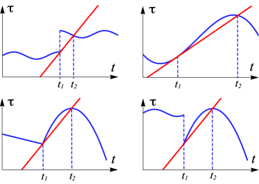
Figure 3: Four ways to enter regime A from regime B. Upper left: when there is a discontinuity in $\tau$ from a low value to a high value. Upper right: when $d\tau/dt$ smoothly goes through the value $d\tau/dt=1$ from whence it increases. Lower left: similar to upper right except that $\tau(t)$ need not be differentiable at the point of entry in A. Lower right: here there is a discontinuity in $\tau$ from a low value to a high value together with a derivative that approaching the point of discontinuity that exceeds unity, $\lim_{t\to t_{1}^{+}}(d\tau/dt)>1$. In all four cases entry into regime A occurs at time $t_{1}$ and exit at time $t_{2}$.

We conclude with a comment: we have indicated that in all cases regime $A$ ends with a re-entry into Regime $B$ in a finite time. This is, in fact, not necessary. Regime $A$ could continue forever. But this would imply a continual growth of $\tau(t)$, which leads to the uninteresting conclusion that (since exit from state $2$ of our array units is forever slowed down) all units will end up in state $2$ and will remain there. This is a trivial dynamics that will not be pursued further.

We end this section by noting that we have so far made no specific assumptions about the functional forms of $\gamma(P_{2}(t))$ or $\tau(P_{2}(t))$ but have, instead, discussed the problem in full generality. We also note that our discussion so far is fully analytic. Now, to proceed we introduce specific forms for these functional dependences.

III The specific model: synchronization

III.1 Choosing a model

At this point any further analysis of the emergence of synchronization in our ensemble of globally coupled oscillators requires us to specify the time-dependent quantities $\gamma(t)$ and $\tau(t)$. For the rate $\gamma$ we choose the standard (Arrhenius-type) exponential law Wood ; Wood2 ; Prager ; Kouvaris

$$\gamma(t) = g\exp\left(\frac{a[N_{2}(t)-N_{1}(t)]}{N}\right)$$ (22)

$$= g\exp\left(\frac{a[2N_{2}(t)-N]}{N}\right).$$

For the refractory period we introduce a non-monotonic dependence on $N_{2}(t)/N$,

$$\tau(t)=\tau_{0}\frac{N_{2}(t)N_{1}(t)}{N^{2}}=\tau_{0}\frac{N_{2}(t)(N-N_{2}(t))}{N^{2}},$$ (23)

which exhibits a maximum when half the units are in state $1$ and the other half in state $2$. An imbalance in either direction shortens the refractory period. Here $g$, $a$ and $\tau_{0}$ are coupling parameters. Next, we can scale time so that with no loss of generality one of the parameters can be fixed, say $g=1$, and hence the system has a total of three free parameters: $a$, $\tau_{0}$ and $N$. We focus on the thermodynamic behavior $N\gg 1$, so that the phase space diagram of the system is, in fact, the two-dimensional parameter plane $\left(a,\tau_{0}\right)$. We have observed that varying just one of these two parameters allows us to capture the main features of the system (the transition to synchronization), so we fix $\tau_{0}=2$ and present our analysis as a function of the coupling parameter $a$.

Note that in principle the coupling parameter may be positive or negative. A positive parameter implies that if many units are in state $1$, say, then they leave that state more slowly than if there are only a few. We choose to study the case of negative $a$, where the behavior is the opposite, namely that units leave state $1$ at a greater rate when it is highly occupied. That is, the system “avoids” crowding. This is consistent with the form chosen for the refractory period: it, is shortened when either state is overcrowded.

III.2 Outcomes in the thermodynamic limit

First we test the mean field theory for our model, that is, we solve Eq. (12), which of course must be done numerically. We observe that after a transient dynamics, the system approaches a long-time behavior that depends on the choice of the coupling parameter $a$. When $|a|$ is small (“small” to be specified accurately later), the system approaches a quiescent state well described by Eq. (16). On the other hand, when the coupling is sufficiently strong (to be determined later), the system either approaches this quiescent state, or, following a transient, the system settles into a globally synchronized dynamics wherein the probabilities $P_{i}(t)$ oscillate in highly anharmonic but essentially periodic fashion. Fig. 4(a) displays a typical such global limit cycle. We thus observe the coexistence of a stationary state and a stable limit cycle. Note that we can not necessarily simply search for initial conditions $P_{2}(0)$ that lead to one behavior or the other. Because the system has a memory, the “basins of attraction” in general would have to be characterized in functional space and require knowledge of $P_{2}(t)$ for past times before $t=0$. For our model, we need to know $P_{2}(t)$ at most in the interval $[-\tau_{0}/4,0]$. If all the units are initially in state $1$, that is, if $P_{2}(0)=0$, then we do not need information about the past. We have not attempted to unravel the functional initial condition problem here.

We test the mean field master equation by also directly simulating the equations of motion of our system. Our simulations here are carried out for $N=10^{4}$. Here again we find that for sufficiently strong coupling, after a transient dynamics the system approaches one of two long-time behaviors: the system either converges to a stationary state wherein $N_{1}$ and $N_{2}$ approach essentially constant values (again well described by the mean field quiescent state (16)), or the system goes to a final state of synchronized dynamics that consists of coherent oscillations of $N_{1}$ and $N_{2}$. The number $N=10^{4}$ is sufficiently large for us not to observe fluctuations that would perturb the system out of an oscillatory dynamical behavior during the time of our simulations, but presumably a sufficiently long run would exhibit such transitions. In any case, we thus again observe the coexistence of a stationary state and a stable limit cycle. Fig. 4(b) displays a typical such global limit cycle, this one for the same initial condition and coupling as in Fig. 4(a). We see that $N_{2}\left(t\right)/N$ exhibits very anharmonic oscillations with well defined amplitude and frequency. The similarity between the two panels reassures us that $N=10^{4}$ is sufficiently large to capture all the essential features of the thermodynamic behavior of the system. The excellent agreement between the solution of the mean field master equation and the direct numerical simulations is gratifying. The simulations inevitably exhibit very small fluctuations not present in the mean field model because the simulations are carried out for finite, albeit large, $N$.

We will subsequently argue that the two solutions, synchronous and asynchronous, are co-existing stable solutions, and that the synchronization is here not related to the destabilization of the stationary state. Regardless of initial condition, a sufficiently strong external disturbance applied to the system can drive it from one state to the other. In a system with a finite number of units the two solutions are metastable states not impervious to fluctuations; indeed, a sufficiently strong fluctuation can cause a transition from one of these states to the other. Thus, now the perturbation need not be external to the system.

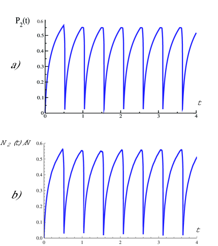
Figure 4: (Color online) Long-time behavior of the model for $a=-2$ and $\tau_{0}=2$. (a) Numerical solution of the mean field equation (12). (b) Direct numerical simulations of the equations of motion for $N=10^{4}$ units coupled according to the prescriptions (22) and (23).

In the next subsection we present a number of results that arise from direct numerical simulations of coupled units. Then, in the next section, we return to the master equation and, to understand the synchronization properties from this more analytic point of view, we construct a Poincaré map for the oscillatory state. Among other results, we calculate the critical coupling for our model in the thermodynamic limit.

III.3 A variety of results of direct numerical simulations

We present several sets of results, not all meant to be quantitatively accurate but rather to illustrate a number of interesting observed features of our system. More detailed studies of these features will be explored in subsequent work subsequent .

First, we illustrate the fact that for small $N$ the fluctuations are sufficiently strong to drive the system back and forth between oscillatory and stationary behavior. We have not explored the dependence of the rate of these transitions on $N$, but note that they arise from the microscopic dynamics. Three realizations of such a progression in time are shown in Fig. 5 for an array of $N=100$ all-to-all coupled units. The precise parameter values are not particularly important other than to confirm that the stationary episodes in the figure are consistent with the stationary value obtained from Eq. (16), which here is $P_{2}^{*}\simeq 0.422$.

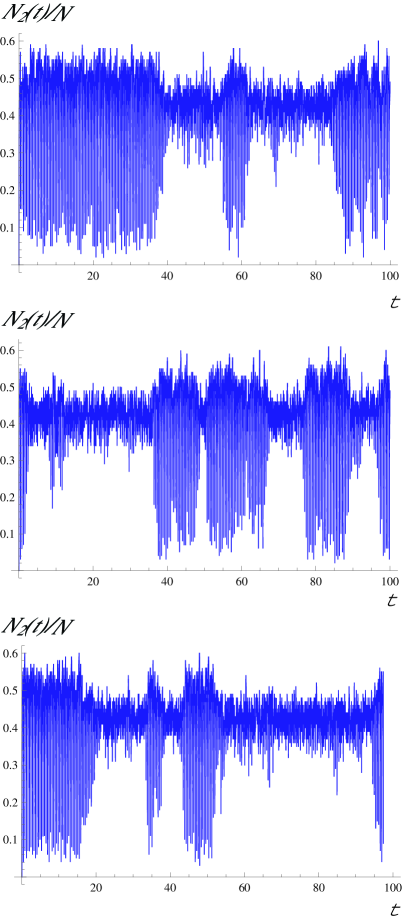
Figure 5: (Color online) Typical realizations for an array of $100$ units coupled according to the prescriptions (22) and (23) above critical coupling. The parameter values are the same for the three realizations. The mean field stationary value for these parameters is $P_{2}^{*}\simeq 0.422$.

A second point to explore is the robustness of the results to variations in the model. Ours would not be a very interesting effort if it depended strongly on the specific features of the model without room for variation. We have explored two specific variations.

To display the first generalization we note that we can express our basic model more generally than we have done, namely, we can introduce a rate $g_{1}(t,t^{\prime})$ of transitions from state $1$ to state $2$, and likewise a rate $g_{2}(t,t^{\prime})$ for transitions from state $2$ back to state $1$. Here $t^{\prime}$ is absolute time, and $t$ denotes the waiting time. We continue to assume that transitions from $1$ to $2$ constitute a Markov process so that $g_{1}(t,t^{\prime})\equiv\gamma(t^{\prime})$ as indicated in Eq. (22). However, for the return we allow a distributed waiting time of the form

$$g_{2}\left(t,\frac{N_{2}\left(t^{\prime}\right)}{N}\right)=\frac{1}{\tau_{0}}\left(\frac{t}{\tau\left(N_{2}\left(t^{\prime}\right)/N\right)}\right)^{b},$$ (24)

which reduces to our working model with a single waiting time when $b\to\infty$. The full master equation is

$$P_{2}(t)= \int_{0}^{\infty}dt^{\prime\prime}\gamma\left(P_{2}(t-t^{\prime\prime})\right)\left(1-P_{2}(t-t^{\prime\prime})\right)$$

$$\times\exp\left(-\int_{0}^{t^{\prime\prime}}\frac{dt^{\prime}}{\tau_{0}}\left(\frac{t^{\prime}}{\tau\left(P_{2}\left(t-t^{\prime\prime}+t^{\prime}\right)\right)}\right)^{b}\right),$$ (25)

which reduces to Eq. (12) with (14) when $b\to\infty$. We have ascertained for various values of $b$ that this also leads to oscillatory solutions for sufficiently strong coupling, that these coexist with stationary solutions in this regime, and that the solutions obtained from the simulations of a large number of coupled units and those obtained from the generalized master equation coincide. The stationary solutions of the master equation satisfy

$$P_{2}^{*}=\frac{C\gamma\left(P_{2}^{*}\right)\left[\tau_{2}\left(P_{2}^{*}\right)\right]^{\frac{b}{b+1}}}{1+C\gamma\left(P_{2}^{*}\right)\left[\tau_{2}\left(P_{2}^{*}\right)\right]^{\frac{b}{b+1}}},$$ (26)

with

$$C=\left[\tau_{0}\left(b+1\right)\right]^{\frac{1}{b+1}}\Gamma\left(\frac{b+2}{b+1}\right).$$

Here $\Gamma$ is the gamma function. It is straightforward to verify that this reduces to Eq. (16) when $b\to\infty$. The oscillatory solutions exhibit the same strongly anharmonic behavior for the values of $b$ we have explored (in the neighborhood of $b=100$) as they do in our working model. A typical realization of such a stationary solution is shown in the upper panel of Fig. 6.

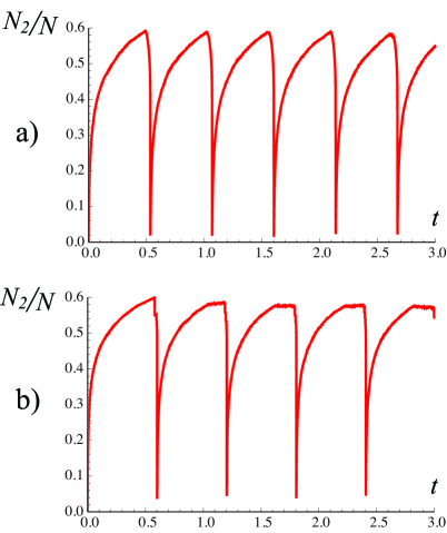
Figure 6: (Color online) (a) Typical realization for direct simulations of the model described in Eqs. (24) and (25) with $\tau_{0}=2$, $a=-4$, $b=100$, and $N=10,000$ coupled according to the prescriptions (22) and (23). (b) Typical realization for model with “displaced waiting time” with parameters $\tau_{0}=2$, $a=-5$, $\delta\tau_{0}=0.1$, and $N=10,000$.

We have also noted that $P_{2}=0$ is a stationary solution of our working model as well as of the generalization discussed above. To vary this, we have explored the consequence of modifying the waiting time in state $2$ from the form $\tau(t)$ of Eq. (23) to $\tau(t)+\delta\tau_{0}$. We have tested the effect of this addition for small values, $\delta\tau_{0}\sim 0.1$, and have again found the same behaviors. A typical realization of an oscillatory solution for this model is seen in the lower panel of Fig. 6.

Finally, we illustrate in Fig. 7 the loss of synchronization with our working model as we cross the critical coupling. The simulation in the figure is for $160,000$ coupled units. In panel (a) the coupling is well above the critical value; in (b) it is just below the critical value, and in (c) it is well below this value.

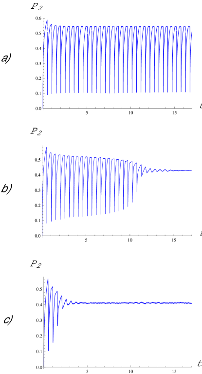
Figure 7: Numerical simulation of $N=160,000$ units: (a) well above critical coupling; (b) just below critical coupling; (c) well below critical coupling.

As promised, we now return to the master equation and, to understand the synchronization properties from this more analytic point of view, we construct a Poincaré map for the oscillatory state so as to obtain a quasi-analytic estimate of the critical coupling in the thermodynamic limit.

IV Poincaré-type map for the oscillatory state

To understand the synchronization properties of our coupled array, and guided by our numerical solutions but proceeding as analytically as possible, we focus on a single typical oscillatory cycle, cf. Fig. 8(a). We define a cycle as the evolution between the two evident discontinuities in the figure, indicated by dashed lines. In more detail, we observe that at the start of a cycle, $P_{2}(t)$ at first grows gradually and then it quickly decreases to a minimum value that is in general different from the starting value of the cycle. Then the process begins again. The cycle shown in Fig. 8 is a generic $n$-th cycle, where $t_{n}$ denotes an arbitrary time which does not play any explicit role in the calculations. The $n$-th cycle starts from some initial condition $P_{2}(t_{n})=p_{n}$ which is the end point of the previous discontinuity (and whose value depends on the past). After a time $T_{2}$ the system undergoes another discontinuity ending at time $t_{n+1}=t_{n}+T_{2}$, that is, $P_{2}(t_{n+1})=p_{n+1}$. Note that $T_{1}$ and $T_{2}$ change from cycle to cycle because periodicity is not perfect, that is, they both depend on $n$ via $p_{n}$. The key to the synchronization is the Poincaré-type map

$$p_{n+1}=f\left(p_{n}\right).$$ (27)

The oscillatory solution corresponds to a fixed point of the map, $p^{*}=f(p^{*})$, and it is stable if $\left|f^{\prime}\left(p^{*}\right)\right|<1$. Otherwise it is unstable StrogatzLib .

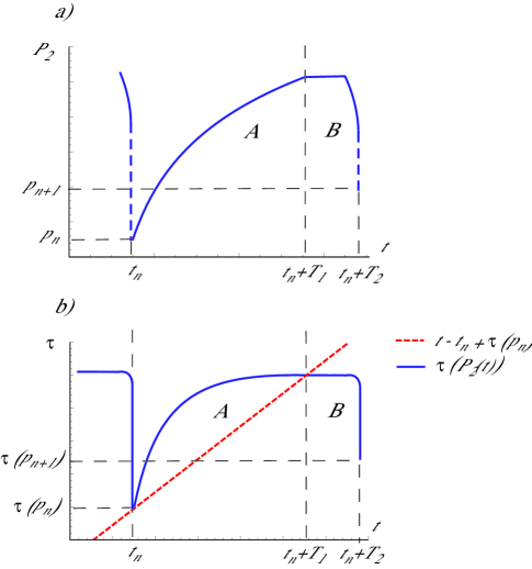
Figure 8: (Color online) (a) $P_{2}$-profile during the $n$-th cycle. (b) Transition delay time $\tau$ vs time (solid, blue), and the straight line $\tau=t-t_{n}+\tau(p_{n})$ vs time (dashed, red). The A portions use the analytic result Eq. (31), while the results for regime B are outcomes of the numerical integration of Eq. (34). Parameter values: $\tau_{0}=2$, $a=-1.5$ and $p_{n}=0.05$ ($p_{n+1}$ was inserted manually in order to clarify the plots).

In order to solve the master equation (12) and compute the map (27), we note that each cycle exhibits two significantly different regimes of behavior, indicated as A and B in Fig. 8. These are precisely the regimes A and B discussed in detail in Appendix A and in Sec. II.

A-regime: This regime is characterized by the fact that the curve $\tau(P_{2}(t))$ lies above the line $t-t_{n}+\tau(p_{n})$, $\tau\left(P_{2}(t)\right)>t-t_{n}+\tau(p_{n})$, for $t_{n}<t<t_{n}+T_{1}$.

B-regime: Here the inequality is reversed (the curve lies below the line), $\tau\left(P_{2}(t)\right)<t-t_{n}+\tau(p_{n})$, for $t_{n}+T_{1}<t<t_{n}+T_{2}$.

We next consider the generalized master equation in each regime separately. Consider first regime A. From Eq. (21) it follows that for $t$ within the interval $[t_{n},t_{n}+T_{1}]$,

$$\Theta(t,t^{\prime})=\theta(t^{\prime}-t_{n}+\tau(t_{n})),$$ (28)

where for economy of notation we have written $\tau(P_{2}(t_{n}))\equiv\tau(t_{n})$. The master equation can then be written as

$$P_{2}^{A}(t)=\int_{t_{n}-\tau(t_{n})}^{t}dt^{\prime}F\left(P_{2}(t^{\prime})\right).$$ (29)

We can alternatively write this in the differential form

$$\dot{P}_{2}^{A}=F\left(P_{2}^{A}\right),$$ (30)

with the initial condition $P_{2}^{A}(t_{n};p_{n})=p_{n}$. The solution is

$$P_{2}^{A}\left(t;p_{n}\right)=1-\frac{1}{2a}\text{ei}^{-1}\left(\text{ei}\left(2a\left(1-p_{n}\right)\right)-e^{a}\left(t-t_{n}\right)\right),$$ (31)

where ei denotes the exponential integral,

$$\text{ei}\left(z\right)=-\int_{-z}^{\infty}du\frac{e^{-u}}{u},$$

and $\text{ei}^{-1}$ denotes its inverse. Hence, in this regime we have presented an exact analytic solution.

We carry this analytic focus further by noting that the A-regime ends after a time interval $T_{1}$, which is defined by the equation

$$T_{1}+\tau\left(p_{n}\right)=\tau\left(P_{2}^{A}\left(T_{1}+t_{n};p_{n}\right)\right),$$ (32)

which identifies the point at which the $\tau$ curve and the line $t-t_{n}+\tau(p_{n})$ intersect. This identification is important because $P_{2}(t)$ reaches a maximum at this point (followed by a plateau discussed below), and with the analytic solution  (31) we can compute this maximum and the time at which it occurs. Note again that $T_{1}$ depends on $p_{n}$, but does not depend on $t_{n}$.

In the B-regime we are forced to rely partly but minimally on numerical simulations, which lead to the observation that $d\tau\left(P_{2}^{B}\left(t;p_{n}\right)\right)/dt<1$. Here we have explicitly indicated the dependence of $\tau$ on $t$ via $P_{2}^{B}$. The master equation in this regime can be written as

$$P_{2}^{B}\left(t;p_{n}\right)=\int_{t-\tau\left(P_{2}^{B}\left(t;p_{n}\right)\right)}^{t}dt^{\prime}F\left(P_{2}\left(t^{\prime};p_{n}\right)\right)$$ (33)

(cf. Eq. (39)). Taking a derivative of this equation with respect to $t$ and solving for $\dot{P}_{2}^{B}(t;p_{n})$ yields the differential form

$$\dot{P}_{2}^{B}(t;p_{n})=\frac{F\left(P_{2}^{B}(t,p_{n})\right)-F\left(\mathcal{P}\left(t-\tau\left(P_{2}^{B}\right)\right)\right)}{1-F\left(\mathcal{P}\left(t-\tau\left(P_{2}^{B}\right)\right)\right)\tau^{\prime}\left(P_{2}^{B}\right)},$$ (34)

where

$$\mathcal{P}\left(t\right)=\left\{\begin{array}[c]{ll}P_{2}^{B}\left(t;p_{n-1}\right)&\text{if }t<t_{n}\\ P_{2}^{A}\left(t;p_{n}\right)&\text{if }t_{n}<t<t_{n}+T_{1}\\ P_{2}^{B}\left(t;p_{n}\right)&\text{if }t>t_{n}+T_{1}\\ \end{array}\right.,$$

together with the initial condition

$$P_{2}^{B}\left(T_{1}+t_{n};p_{n}\right)=P_{2}^{A}\left(T_{1}+t_{n};p_{n}\right).$$ (35)

Equation (34) is a non-autonomous differential equation for $t-\tau\left(P_{2}^{B}\left(t;p_{n}\right)\right)<t_{n}$ because it depends on $P_{2}^{B}$ in the previous cycle, $P_{2}^{B}(t;p_{n-1})$. It is also non-autonomous for $t_{n}<t-\tau\left(P_{2}^{B}\left(t;p_{n}\right)\right)<t_{n}+T_{1}$ because it depends on $P_{2}^{A}$ in the same cycle, $P_{2}^{A}(t;p_{n})$. In general, for $t-\tau\left(P_{2}^{B}\left(t;p_{n}\right)\right)>t_{n}+T_{1}$ it is a delay differential equation Wiener because it only $P_{2}^{B}$ at previous times; however, as seen immediately below, this regime is not reached in our system in the oscillatory state.

More specifically for our case, the description of the system in regime B then proceeds as follows. For $t-\tau\left(P_{2}^{B}\left(t;p_{n}\right)\right)<t_{n}$, the $P_{2}$-profile exhibits a plateau as seen in Fig. 8(a). Note that this is a word used here to describe a numerical observation rather than an analytic precise outcome. Then, for $t_{n}<t-\tau\left(P_{2}^{B}\left(t;p_{n}\right)\right)<t_{n}+T_{1}$ it quickly decreases up to the time at which it exhibits the discontinuity. This occurs at $t_{n}+T_{2}$, which satisfies $T_{2}-\tau\left(P_{2}^{B}\left(t_{n}+T_{2};p_{n}\right)\right)<T_{1}$. Equation (34) remains a non-autonomous differential equation during this entire portion of the cycle, that is, it reaches the discontinuity before it becomes a delay differential equation.

At the level of Eq. (34) the discontinuity is related to the divergence $\dot{P}_{2}^{B}\left(t\rightarrow t_{n}+T_{2};p_{n}\right)\rightarrow-\infty$. At the discontinuity, $P_{2}(t)$ falls to the value $p_{n+1}$, and regime A begins again,

$$p_{n+1}=P_{2}^{A}(t_{n+1};p_{n+1}).$$ (36)

We also note that numerical simulations show that $p_{n}$ is small, so that we can assume that $T_{2}-\tau(t_{n+1})>T_{1}$. In this case, $t$ lies in the range,$[t_{n}+T_{2}-\tau(t_{n+1}),t_{n}+T_{2}]$. This places us in regime B of cycle $n$. We can thus write

$$p_{n+1}=\int_{t_{n+1}-\tau(p_{n+1})}^{t_{n+1}}dt^{\prime}F\left(P_{2}^{B}(t^{\prime};p_{n})\right)$$ (37)

where $t_{n+1}=t_{n}+T_{2}$ and where we have invoked Eqs. (37) and (29). This is an equation that relates $p_{n+1}$ to $p_{n}$, that is, it implicitly contains the map (27).

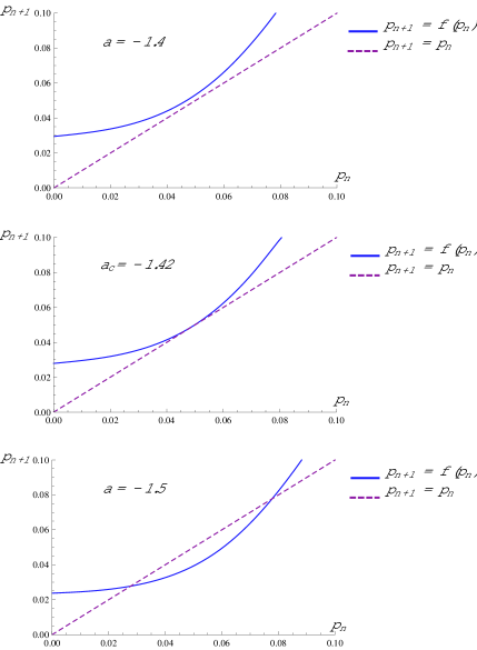
Figure 9: (Color online) Computation of the map (27) for $\tau_{0}=2$ and three different values of $a$.

To compute the map we have again combined numerical with analytical results by numerically solving Eqs. (34) and (37) using the analytic solution for $P_{2}^{A}(t;p_{n})$. Our results for $\tau_{0}=2$ are summarized in Fig. 9, which clearly predicts that synchronization appears via a saddle node bifurcation. For $a>a_{c}$ the function $f$ has no fixed points, so the system is not able to synchronize. At $a=a_{c}$ the function $f$ just touches the line $p_{n+1}=p_{n}$, and for $a<a_{c}$ there appear two fixed points related to periodic orbits. The lower fixed point corresponds to the stable oscillation that we observe in our simulations; the other fixed point corresponds to an unstable limit cycle. From this analysis we find that the critical point for $\tau_{0}=2$ occurs at $a_{c}=-1.42$.

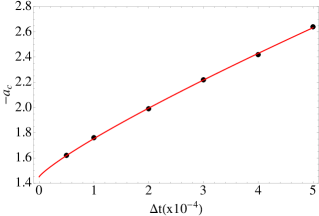
Figure 10: (Color online) Variation of the critical point with the integration step size $\Delta t$ (see text). The continuous curve is the best power law fit to the numerical data, $-a_{c}=0.303(\Delta t)^{0.846}+1.44$. Extrapolating to $\Delta t\to 0$ leads to the critical point $a_{c}=-1.44$, which is close to the value $a_{c}=-1.42$ obtained from the saddle node analysis of the master equation.

We can also estimate the critical point directly from the integral equation (12). To arrive at an ever more accurate critical point via this route, we must use ever smaller time steps $\Delta t$ in the numerical integration. In Fig. 10 we present the results as we decrease the time step, and obtain the value $a_{c}=-1.44$ upon extrapolation to $\Delta t\to 0$. The two methods to calculate the critical point thus show a high level of agreement.

V Conclusions

It is well known that a globally syncrhonized state can not occur in Markovian arrays of coupled two-state systems. A number of models of coupled arrays of two-state units have been constructed that depart in one way or another from Markovian dynamics and that as a result do lead to global synchronization. These models share a feature: the memory lies in the coupling between units and does not affect the dynamics of the units themselves.

We have here constructed a novel departure from Markovian behavior that also leads to globally synchronized dynamics, and that incorporates a physical feature endemic to two-state systems: a refractory period. Specifically, in our model the single units are not Markovian to begin with but instead, upon arrival at one of the two states, they are subject to a delay time before they can return to the other state. The coupling among units is reflected in a state dependence of this delay time. In other words, the refractory period itself is affected by the state of the system and therefore changes with time.

In this globally coupled array we have found a synchronized state that exhibits highly anharmonic dynamics with cyclical discontinuities. The global dynamics of the network can be described by a generalized master equation. We have solved the generalized master equation to show that this type of synchronization is the result of a saddle node bifurcation in the phase space of the system. The critical coupling strength, as well as the amplitude and period of oscillations, are derived analytically by explicitly solving the generalized master equation. We find that as we approach the critical coupling parameter $a_{c}$ from below, transient oscillatory behavior of longer and longer duration $T$ occurs, with $T\to\infty$ as $a\to a_{c}$. We are currently exploring the functional dependence of $T$ on $|a-a_{c}|$.

The main points to be emphasized can be summarized as follows. Incorporating a refractory period that depends on the global state of the system has given rise to a rich dynamics, one that can exhibit oscillations and coexistence between the synchronous and asynchronous states (bistability). The nature of the synchronization that leads to self-organization far from equilibrium is here not related to the destabilization of the thermodynamic branch. Indeed, this branch, which leads to stationary behavior, remains stable and coexists with the stable oscillatory branch. This is an entirely different synchronization paradigm than that obtained from the usual Hopf bifurcation and the attendant destabilization of the thermodynamic stationary state. We have ascertained that our model is robust by considering two variations of the model and showing that all three models lead to similar synchronization properties.

Refractory properties are evident in a large variety of systems ranging from the physiological (refractory properties of an excitable membrane) to the physical (blinking quantum dots). The rich dynamics of our simple on-off model makes this an excellent candidate for adaptation to specific applications.

Appendix A Generalized master equation for mean field coupling

In this Appendix we explore possible explicit functional forms of $\tau$ and the concomitant behavior of $\Theta$. Note that we are ultimately especially interested in finding the long-time behavior of the coupled array. To make the case clear, we build up from the simplest possible scenarios to the most complex that we will encounter.

Consider first the case of a function $\tau(P_{2}(t))$ that decreases smoothly with time, as sketched in the upper left panel of Fig. 11. The construct in the sketch clearly shows that the inequality is valid only at the foot of the triangle. Units that arrived earlier than $t-\tau(t)$ will have left before time $t$ and thus do not obey the inequality. The $\Theta$ function can then be expressed in the simple form

$$\Theta(t,t^{\prime})=\theta\left(t^{\prime}-t+\tau(P_{2}(t))\right),$$ (38)

where $\theta$ is the Heaviside step function. The resultant master equation reads

$$P_{2}(t)=\int_{t-\tau(P_{2}(t))}^{t}dt^{\prime}F\left(P_{2}(t^{\prime})\right).$$ (39)

If $\tau(t)$ increases smoothly with time, then the same analysis is valid provided $d\tau/dt\leq 1$. This is apparent in the schematic in the upper right panel of the figure. Indeed, the master equation (39 is valid for non-monotonic continuous functions $\tau(t)$ even if there are discontinuities in its time derivative, provided $d\tau/dt\leq 1$, cf. lower panel of Fig. 11.

In summary, as long as $\tau(t)$ is a continuous function of time and $d\tau/dt\leq 1$ we find that Eq. (38) holds, which in turn implies the master equation (39). This is of course in general a complicated equation for $P_{2}(t)$, nonlinear and nonlocal in time.

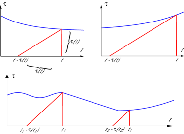
Figure 11: Left upper panel: Schematic of the construct leading to the generalized master equation Eq. (39) when $\tau(P_{2}(t))$ is analytic and decreasing with time. Right upper panel: The corresponding schematic when $\tau(t)$ is analytic and increasing with time. The master equation (39) again results provided $d\tau/dt<1$. Lower panel: again Eq. (39) applies for continuous $\tau(t)$ even if there are discontinuities in its derivative, provided $d\tau/dt<1$.

Next let us suppose that $\tau(t)$ itself has discontinuities. Two generic situations are possible, as shown in Fig. 12. First consider a discontinuous abrupt decrease of $\tau$ at $t\equiv t_{D}$ from a high value of $\tau_{-}$ to the left of the discontinuity to a low value $\tau_{+}$ to the right, as seen in the upper panels. For later reference we call this Case 1. The behavior away from $t_{D}$ on either side may be as described above, in which case it requires no extra analysis, or increases with time and violates the condition $d\tau/dt<1$, a case discussed subsequently. In any case, we must be careful as we approach $t_{D}$. The sketch in the upper left panel of Fig. 12 shows that approaching $t_{D}$ from below gives

$$\lim_{t\to t_{D}^{-}}\Theta(t,t^{\prime})=\theta(t^{\prime}-t_{D}+\tau_{-}).$$ (40)

Approaching the discontinuity from above (right upper panel) leads to

$$\lim_{t\to t_{D}^{+}}\Theta(t,t^{\prime})=\theta(t^{\prime}-t_{D}+\tau_{+}).$$ (41)

Thus we see that $\Theta$ inherits the discontinuity of $\tau(t)$, but this is automatically “built in” in Eq. (38), which is still valid. Hence the generalized master equation is again given by Eq. (39).

Now suppose the discontinuity occurs in the opposite direction, from a low value $\tau_{-}$ to a high value $\tau_{+}$ as we move from left to right. This is shown in the lower panels of Fig. 12. We call this Case 2. Again, sufficiently far from the discontinuity either the previous discussion surrounding Fig. 11 continues to hold, or the subsequent discussion does. As we approach $t_{D}$ from the left all continues as before up to the value $t^{\prime}=t_{D}-\tau_{-}$,

$$\lim_{t\to t_{D}^{-}}\Theta(t,t^{\prime})=\theta(t^{\prime}-t_{D}+\tau_{-}).$$ (42)

This is clarified in the left lower panel of Fig. 12. However, when $t^{\prime}$ lies in the interval $[t_{D}-\tau_{+},t_{D}-\tau_{-}]$ then for $t"$ in the range $[\bar{t},t_{D}]$ lying between $t^{\prime}$ and $t_{D}$ we see from the figure that the inequality is not satisfied, i.e. that $t^{\prime}-t^{\prime}>\tau(t")$. Here $t^{\prime}-\bar{t}=\tau(\bar{t})$. However, when $t"$ continues to move up within the range $[t^{\prime},t_{D}]$, the inequality is once again satisfied, $t^{\prime}-t<\tau(t")$. The change from “not satisfied” to “satisfied” occurs at the value $t^{\prime}=t_{D}-\tau_{-}$, so that

$$\lim_{t\to t_{D}^{+}}\Theta(t,t^{\prime})=\theta(t^{\prime}-t_{D}+\tau_{-}).$$ (43)

Comparing the last two equations, we see that $\Theta$ is now in fact continuous in spite of the discontinuity in $\tau(t)$, that is, $\Theta$ now does not inherit the discontuity as it did when $\tau(t)$ abruptly decreases. This asymmetry in behavior is of course a consequence of the direction of the arrow of time.

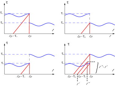
Figure 12: Cases that can arise when $\tau(t)$ has discontinuities. Upper panels: high to low discontinuities. Lower panels: low to high discontinuities.

Furthermore, additional “different” behavior is observed as we continue further upward in time. Suppose we now look at values of $t$ in the next range, $[t_{D},t^{*}]$, where $t^{*}$ satisfies the equation

$$t^{*}-(t_{D}-\tau_{-})=\tau(t^{*}).$$ (44)

The inequality is satisfied for all $t$ in this range provided that $t^{\prime}-t<\tau_{-}$, that is,

$$\lim_{t\to t_{D}^{+}}\Theta(t,t^{\prime})=\theta(t^{\prime}-t_{D}+\tau_{-}).$$ (45)

Comparing Eq. (45) with Eq. (43) reveals a remarkable behavior: provided $t\in[t_{D},t^{*}]$, $\Theta(t,t^{\prime})$ does not depend on $t$! Beyond $t^{*}$ the behavior as expected from our analysis of a smooth function $\tau(t)$ is recovered.

References

- (1) R. C. Elson, et al, Phys. Rev. Lett. 81, 5692 (1998).
- (2) J. D. Murray, Mathematical Biology (Springer-Verlag, Berlin, 1989).
- (3) P. Frantsuzov, M. Kuno, B. Janko, and R. A. Markus, Nature Physics 4, 519 (2008); P. A. Frantsuzov, S. V.-Kacso, and B. Janko, Phys. Rev. Lett. 103, 207402 (2009).
- (4) H. Zhou and R. Lipowsky, PNAS 105, 10052, (2005).
- (5) L. Glass, Nature 410, 277 (2001).
- (6) A. Pikovsky, M.. Rosenblum and J. Kurths, “Synchronization: A Universal Concept in Nonlinear Sciences”, Cambridge (2001).
- (7) K. Wiesenfeld, P. Colet and S. Strogatz, Phys. Rev. Lett. 76, 404 (1996).
- (8) K. Wood, C. Van den Broeck, R. Kawai, and K. Lindenberg, Phys. Rev. Lett. 96, 145701, (2006); K. Wood, C. Van den Broeck, R. Kawai, and K. Lindenberg, Phys. Rev. E 74, 031113, (2006).
- (9) K. Wood, C. Van den Broeck, R. Kawai, and K. Lindenberg, Phys. Rev. E 76, 041132, (2007).
- (10) T. Prager, B. Naundorf and L. Schimansky-Geier, Physica A 325, 176 (2003); T. Prager, M. Falcke, L. Schimansky-Geier and M. A. Zaks, Phys. Rev. E 76, 011118, (2007).
- (11) N. Kouvaris, F. Miller and L. Schimansky-Geier, Phys. Rev. E 82, 061124, (2010).
- (12) B. Blasius, A. Huppertand L. Stone, Nature 399, 354 (1999); B. Blasius and L. Stoney, Int. J. Bifurcation and Chaos 10, 2361 (2000).
- (13) S. Strogatz, “Nonlinear Dynamics and Chaos”, Perseus, Massachusetts (1994).
- (14) D. Pazó, Phys. Rev. E 72, 046211 (2005).
- (15) M. K. S. Yeung and S. H. Strogatz, Phys. Rev. Lett. 82, 648, (1999); E. Montbrio, D. Pazo and J. Schmidt, Phys. Rev. E. 74, 056201, (2006).
- (16) D. Huber and L. S. Tsimring, Phys. Rev. Lett. 91, 260601, (2003).
- (17) F. Julicher and J. Prost, Phys. Rev. Lett. 78, 4510, (1997).
- (18) T. Danino, O. M.-Palomino, L. S. Tsimring and J. Hasty, Nature 463, 326 (2010); W. Mather, M. R. Bennet, J. Hasty and L. S. Tsimring, Phys. Rev. Lett. 102, 068105 (2009); D. Bratsun, D. Wolfson, L. S. Tsimring and J. Hasty, PANS 102, 14593 (2005).
- (19) F. Rozenblit and M. Copelli, J. Stat. Mech. 2011, P01012.
- (20) J. Wiener and J. K. Hale, “Ordinary and Delay Differential Equations”, Wiley, New York (1992).
- (21) U. Harbola, D. Escaff, and K. Lindenberg, In preparation.