A new perspective on Gauge-flation

Abstract

Recently Maleknejad and Sheikh-Jabbari have proposed a new model for inflation with non-Abelian gauge fields (Gauge-flation), and they have studied the model by numerical methodsSheikh . In this model, the isotropy of space-time is recovered by suitable combination of gauge configurations, and a scalar field is constructed by gauge field and the scale factor, which produces inflation period. In this work, exact solutions for the scalar field and the Hubble parameter are presented and we provide analytic solutions for the numerical results. We explicitly present Hubble parameter and fields as functions of time and it is also demonstrated that in some conditions they are damped oscillator. Moreover, reheating period in the model is discussed.

I INTRODUCTION

Observations of the cosmic microwave background and large scale structure are consistent with the isotropic symmetry of space-time and inflation Weinberg , a period of accelerated expansion occurring in early universe. To save isotropic symmetry of background space-time, many models use a single or multi-scalar field(s)(inflaton) with ansatz that the inflaton field rolls slowly down its potential (inflationary period) Weinberg . Eventually the field(s) oscillates around the minimum of its potential and decays into light particles(reheating period). It has been assumed that reheating period took place just after inflationary period and the field behaved like dust matter in the reheating period Weinberg .
We have had few models that can be solved exactly in the cosmological context. The well-known example, that can be solved exactly, is the exponential potential Weinberg ; Ratra which, with suitable parameters, gives us inflationary solution(power law inflation). Usually, solving field equations are limited to either the inflationary period, with slow roll approximations, or reheating period.
The success of gauge symmetry in the standard particle physics shows that the gauge symmetry is the correct tool to construct an effective field theory. But, at first glance, it seems impossible to reconcile the isotropic symmetry with the vectorial nature of gauge fields. However, recently a new model for inflation, Gauge-flation, based on gauge field , $\displaystyle A_{~{}\mu}^{a}$, where $\displaystyle a,b,\ldots$ and $\displaystyle\mu,\nu,\ldots$ are used for the indices of gauge algebra and the space-time respectively, has been proposed by Maleknejad and Sheikh-Jabbari(MS) Sheikh . The rotational symmetry in 3d space is retained by introducing three gauge fields, such that these gauge fields rotate among each other by $\displaystyle SU(2)$ non-Abelian gauge transformations Sheikh . In this model, a scalar field that causes inflation period, $\displaystyle\psi$, is constructed from the gauge field and the scale factor (see below). MS have studied the model by numerical analysis and obtained numerical solutions for the model Sheikh .
In this work we investigate the model by analytic method. As we will see, the model has some features that allow us to obtain leading order of fields in all epochs of the universe and not just only in a specific period. We provide an analytic expression for MS solutions and we study reheating period in this model.
This letter is organized as follows: in §II we briefly review the model and obtain equations in terms of variables which we will use in this letter. In §III we consider a special solution in spectrum of solutions of the model, that the equations can be solved exactly. The solution yields analytic expression for the Hubble parameter and fields for all epochs of the universe. Also we give the general form of solutions for the fields. In §IV we obtain the analytic form for the MS solutions. Constraints on the solutions from slow roll conditions and observations are discussed in §V. In §VI we discuss about reheating period in the model. We summarize our finding in §VII. In Appendix A, we obtain the equation of motion of fields in terms of variables that we use in this letter.

II The model

We work with a general flat-space FRW background metric with signature $\displaystyle(-+++)$, and reduced Plank unites $\displaystyle 8\pi G=1$. Following Sheikh , we consider the effective Lagrangian,

$${\cal L}=\sqrt{-g}\left(-\frac{R}{2}-\frac{1}{4}F^{a}_{~{}\mu\nu}F_{a}^{~{}\mu\nu}+\frac{\kappa^{2}}{384}(\epsilon^{\mu\nu\lambda\sigma}F^{a}_{~{}\mu\nu}F^{a}_{~{}\lambda\sigma})^{2}\right),$$ (1)

where $\displaystyle\epsilon^{\mu\nu\lambda\sigma}$ is the totally antisymmetric tensor and the strength field $\displaystyle F$ is

$$F^{a}_{~{}\mu\nu}=\partial_{\mu}A^{a}_{~{}\nu}-\partial_{\nu}A^{a}_{~{}\mu}-g\epsilon^{a}_{~{}bc}A^{b}_{~{}\mu}A^{c}_{~{}\nu}\quad,$$ (2)

where $\displaystyle\epsilon_{abc}$ is the totally antisymmetric tensor. Sheikh-Jabbari Sheikh2 has shown how $\displaystyle F^{4}$ term in (1) is obtained by integrating out a massive axion field in Chromo$\displaystyle-$Natural inflation Chromo-Natural Inflation . Also, it has been argued how other dimension 8 level terms are suppressed Sheikh2 .
To retain isotropy symmetry of space-time we have to set Sheikh

$$A^{a}_{~{}\mu}=\left\{\begin{array}[]{ll}\phi(t)\delta^{a}_{i}\,,&\mu=i\\ 0\,,&\mu=0\,.\end{array}\right.$$ (3)

Applying Einstein’s equations with this setup results in Sheikh

$$\begin{split}\dot{H}&+2H^{2}=\kappa^{2}\frac{g^{2}\phi^{4}\dot{\phi}^{2}}{a^{6}},\cr\dot{H}~{}&=-(\frac{\dot{\phi}^{2}}{a^{2}}+\frac{g^{2}\phi^{4}}{a^{4}})\,,\end{split}$$ (4)

where $\displaystyle a$ is the scale factor. The equation of motion for $\displaystyle\phi$ is obtained by combination of the equations in(4) Sheikh , so it is not an independent equation and we take (4) to study the model . Neither $\displaystyle\phi(t)$ nor $\displaystyle a(t)$ are scalar under general coordinate transformation, while $\displaystyle\psi(t)=\phi(t)/a(t)$ is a scalar, so we seek solutions for it. We define a new variable $\displaystyle\alpha(t)$ by writing

$$\begin{split}\frac{\dot{\phi}}{aH}&=\sqrt{\epsilon(t)}\hskip 3.61371pt\cos\alpha(t),\cr\frac{g\phi^{2}}{a^{2}H}&=\sqrt{\epsilon(t)}\hskip 3.61371pt\sin\alpha(t),\end{split}$$ (5)

where $\displaystyle\epsilon(t)\equiv-\dot{H}/{H^{2}}$ and $\displaystyle\alpha(t)$ is an arbitrary function of time. Using (5), the system of equations in (4) is reduced to

$$2-\epsilon(t)=\frac{\kappa^{2}}{4}\epsilon^{2}(t)H^{2}\sin^{2}2\alpha(t),$$ (6)

noting that $\displaystyle 0<\epsilon(t)\leq 2$. Without assumption either on the $\displaystyle H$ or on the $\displaystyle\alpha(t)$ Eq. (6) cannot be solved to obtain an expression for the Hubble parameter as a function of time(except for $\displaystyle\kappa=0$ that results in $\displaystyle H=1/2t$, ”radiation epoch”). To explore the model, we define

$$H\sin 2\alpha(t)\equiv\beta f(t),$$ (7)

where $\displaystyle\beta$ is an arbitrary number (dimensionless in Plank units), but $\displaystyle\beta\leq H$.
As we will see, the MS solutions can be obtained by a special form for the $\displaystyle f(t)$. Before we study the MS solution we take a ”simple” ansatz for $\displaystyle f(t)$, that not only helps us to understand the MS solutions, but also, it gives information about dynamics of the model.

III The simple ansatz

In this section we use the following simple form for $\displaystyle f(t)$

$$f(t)=\sin\omega t,$$ (8)

where $\displaystyle\omega$ is an arbitrary number. Using Eqs. (6) and (8), we have

$$\epsilon(t)=\frac{\sqrt{1+2k\sin^{2}\omega t}-1}{\frac{k}{2}\sin^{2}\omega t},$$ (9)

where $\displaystyle k\equiv(\kappa\beta)^{2}$. Note that $\displaystyle\displaystyle\lim_{\omega t\to n\pi}\epsilon(t)=2$, where $\displaystyle n$ is an integer number. $\displaystyle\epsilon(t)$ is a periodic function of time and for $\displaystyle k>4$ it crosses $\displaystyle\epsilon(t)=1$ line (acceleration expansion phase), and for $\displaystyle k>8\times 10^{4}$ it crosses $\displaystyle\epsilon(t)=10^{-2}$ line. The $\displaystyle\epsilon(t)$ is designed as in Fig. 1.
To understand behaviour of $\displaystyle\epsilon(t)$, we can derive an useful formula for $\displaystyle\epsilon(t)$ in inflationary period(i.e., when $\displaystyle\epsilon(t)\ll 1$). From Eqs. (6) and (7), $\displaystyle\epsilon(t)$ in this limit becomes

$$\epsilon(t)\approx\frac{\sqrt{8}}{\sqrt{k}\sin\omega t_{inf}},$$ (10)

where the subscript ”$\displaystyle inf$” denotes that the above expression is valid when $\displaystyle\epsilon(t)\ll 1$, i.e., $\displaystyle 0<\omega t_{inf}<\pi$. For large value for $\displaystyle k$, the validity of Eq. (10) is broken when $\displaystyle t$ is very close to $\displaystyle n\pi/\omega$, so the universe almost evolves through acceleration expansion phases for $\displaystyle k\gg 1$, but eventually exits abruptly from inflationary period, as indicated in Fig. 1.

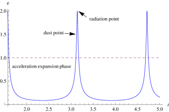
Figure 1: The $\displaystyle\epsilon(t)$ versus $\displaystyle t$ for $\displaystyle k=10^{6}$, $\displaystyle\omega=2$. After inflation, the universe exits abruptly from inflationary period.

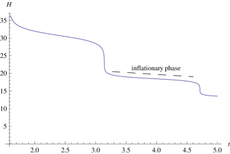
Figure 2: The Hubble parameter versus $\displaystyle t$ for $\displaystyle k=10^{6}$, $\displaystyle\omega=2$. Since $\displaystyle-\dot{H}$ increases with time, the second steep slope is shorter than the first steep slope.

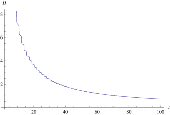
Figure 3: The Hubble parameter versus $\displaystyle t$ for $\displaystyle k=10^{6}$, $\displaystyle\omega=2$.

Integration of (9) gives

$$\begin{split}H(t)={k\omega}\biggr{/}2\biggr{(}&\left(1-\sqrt{1+k(1-\cos 2\omega t)}\right)\cot\omega t\quad+\\ &(1+2k)F[\omega t\,|\!-2k]-E[\omega t\,|\!-2k]\biggr{)},\end{split}$$ (11)

where $\displaystyle F[\omega t\,|\!-2k]$ and $\displaystyle E[\omega t\,|\!-2k]$ are elliptic integrals of the first and second kind respectively and the specific combination of them in (11) is increased monotonically with time Abramowitz . Also

$$\lim_{t\to\frac{n\pi}{\omega}}\left((-1+\sqrt{1+k(1-\cos 2\omega t)}\right)\cot\omega t=0,$$ (12)

so the Hubble parameter is damped (but it is singular at $\displaystyle t=0$). The Hubble parameter is planned as in Fig. 2 and Fig. 3, where it has gentle slopes when $\displaystyle\epsilon<1$( inflationary phase). Since $\displaystyle H$ is decreased with time and $\displaystyle\epsilon(t)$ is a periodic function of time, we conclude that not only $\displaystyle\dot{H}<0$ but also $\displaystyle-\dot{H}$ is decreased with time, as indicated in Fig. 2.
If we demand just one inflationary phase for the universe and define $\displaystyle\Delta t_{inf}$ as the duration of time that inflation takes place, from (10) we have

$$\omega\Delta t_{inf}<\pi.$$ (13)

Note that (13) is the upper bound on $\displaystyle\omega\Delta t_{inf}$ that the model predicts itself and it must be consistent with observational constraints (see below).
From Eqs.(5) and (7), we find

$$\psi_{\pm}^{2}(t)=\frac{H\sqrt{\epsilon(t)}}{g}\left(\frac{1\pm\sqrt{1-\frac{\beta^{2}\sin^{2}\omega t}{H^{2}}}}{2}\right)^{\frac{1}{2}},$$ (14)

where $\displaystyle\epsilon(t)$ and $\displaystyle H$ are given by (9) and (11) respectively.
It is worth to mention that our results in (9), (11) and (14) are valid for all values of $\displaystyle\epsilon(t)$ and this is one of the interesting properties of the model compared with other models for inflation, which use $\displaystyle\epsilon(t)$ as a perturbation parameter and their solutions for the Hubble rate or field(s) are limited to a specific epoch (inflationary period or reheating period). In this sense, the above expressions are exact(non-perturbative) and nonsingular solutions of nonlinear equations (4).
The inverse proportionality of $\displaystyle\psi_{\pm}$ to $\displaystyle\sqrt{g}$, shows that they are not exist in perturbation regime.
To understand the behaviour of (14) , we use the fact that $\displaystyle\beta\leq H$, and expand (14) that gives

$$\psi_{+}^{2}(t)=\frac{H\sqrt{\epsilon(t)}}{g}\qquad,\hskip 21.68121pt\psi_{-}^{2}(t)=\frac{\beta\sqrt{\epsilon(t)}}{2g}\sin\omega t.$$ (15)

Here the higher terms $\displaystyle\sim\beta^{2}/H^{2}$ have been neglected. So, $\displaystyle\psi_{+}$ is damped oscillator and $\displaystyle\psi_{-}$ is oscillator (till $\displaystyle\beta\leq H$). The leading order behaviour of $\displaystyle\psi^{4}_{\pm}$ are sketched in Fig. 4.
Recall that in the reduced Plank units, $\displaystyle H<1$( after Plank time), and $\displaystyle\beta<H$, so $\displaystyle\psi_{-}$ is smaller than $\displaystyle\psi_{+}$ in the inflation period. However, from the Friedman equation, $\displaystyle\rho_{\psi_{\pm}}=3H^{2}$, we realise that both of them have the same density, and the behaviour of $\displaystyle H$ (in Eq. (11) and Fig. 3) shows that the cosmic expansion dilutes the density of fields, although the expectation value of $\displaystyle\psi_{+}$ is greater than $\displaystyle\psi_{-}$ after inflation.
For general type of $\displaystyle f(t)$ in (7), $\displaystyle H$ cannot be obtained in terms of well-known functions, but by algebraic manipulations of equations (5),(6) and (7), one can show that for leading order of fields we have

$$\psi_{+f}^{2}(t)=\frac{H_{f}\sqrt{\epsilon(t)}}{g}\qquad,\hskip 14.45377pt\psi_{-f}^{2}(t)=\frac{\beta\sqrt{\epsilon(t)}}{2g}f(t),$$ (16)

where $\displaystyle H_{f}$ is the Hubble rate for $\displaystyle f(t)$. Since $\displaystyle H_{f}$ is usually unknown, the above expression is formal for $\displaystyle\psi_{+f}$ , but the leading order of $\displaystyle\psi_{-f}$ is given by (16) for any $\displaystyle f(t)$.
Note that Eqs. (16) are valid for all values of $\displaystyle\epsilon(t)$. The physical meaning of $\displaystyle f(t)$ is clear from (16), i.e., $\displaystyle f(t)$ shows boundary conditions on the fields.

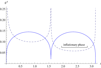
Figure 4: The leading order behaviour of $\displaystyle\psi^{4}_{-}$ (solid line) and $\displaystyle\psi^{4}_{+}$ (dashed line) for $\displaystyle k=10^{6}$, $\displaystyle\omega=2$, $\displaystyle\beta=g=10^{-6}$

IV The MS solutions

We pointed out that MS have analysed the model by numerical methods. Here we will show that to rederive the results we must take the following form for $\displaystyle f(t)$

$$f(t)=\left(\frac{\sin(\alpha_{1}t+\alpha_{2}t^{2}+\cdots)}{\alpha_{1}t}\right)^{2}\equiv f_{MS}(t),$$ (17)

$\displaystyle\epsilon(t)$ and the leading order of $\displaystyle\psi_{-}$ are obtained by (6), (7), (16) and (17) as

$$\begin{split}&\epsilon_{MS}(t)=\frac{2\left(\sqrt{1+2kf^{2}_{MS}(t)}-1\right)}{kf^{2}_{MS}(t)},\cr~{}&\psi_{-MS}^{2}(t)=\frac{\beta\sqrt{\epsilon(t)}}{2g}f_{MS}(t)\,.\end{split}$$ (18)

Figures 5 and 6 are obtained by our analytic method and they have the same pattern as MS have obtainedSheikh .
Note that if $\displaystyle f_{MS}\to 0$ then $\displaystyle\epsilon(t)=2$. Although in this case we cannot obtain an exact expression for the Hubble parameter (for all time), but with (17), we can obtain some information about the MS solution in various regimes.
The most important coefficient of (17) in inflationary phase is $\displaystyle\alpha_{1}$. When $\displaystyle\alpha_{1}t<1$ we have $\displaystyle f(t)\approx 1$, so in this regime from (17) and (18), we have

$$\epsilon_{MS}(t)\approx\frac{2(\sqrt{1+2k}-1)}{k},$$ (19)

i.e., $\displaystyle\epsilon_{MS}(t)$ is constant in this regime as indicated in Fig. 5. To have $\displaystyle\epsilon(t)\ll 10^{-2}$, we must take $\displaystyle k\gg 8\times 10^{4}$.
Therefore the Hubble parameter in this regime is

$$H_{MS}(t)\approx\frac{k}{2(\sqrt{1+2k}-1)t}.$$ (20)

Hence, from (16) and (19) it follows that

$$\begin{split}\psi_{+MS}^{2}(t)&\approx\sqrt{\frac{k}{2g^{2}(\sqrt{1+2k}-1)}}\hskip 2.168pt\frac{1}{t},\cr\psi_{-MS}^{2}(t)~{}&\approx\frac{\beta}{2g}\sqrt{\frac{2(\sqrt{1+2k}-1)}{k}},,\end{split}$$ (21)

so, the leading order of $\displaystyle\psi_{-}$ is constant in this regime, as indicated in Fig. 6.
When $\displaystyle\alpha_{1}t\approx\pi$, the numerator in (17) equals to zero, and therefore $\displaystyle\epsilon_{MS}\to 2$. Just like the simple ansatz in §II, for large $\displaystyle k$, the universe almost evolves through inflation period but eventually exits abruptly when $\displaystyle t\to\pi/\alpha_{1}$.
Using (17), the Taylor expansion of $\displaystyle\epsilon(t)$ in (18) around $\displaystyle t=\pi/\alpha_{1}$ is

$$\epsilon_{MS}(t)\approx 2-\frac{\alpha^{4}_{1}k}{\pi^{4}}(t-\frac{\pi}{\alpha_{1}})^{4},$$ (22)

The Hubble parameter in this regime can be derived by integration of (22), that is

$$H_{MS}(t)\approx\frac{1}{2t}\left(1+\frac{\alpha^{4}_{1}k}{10\pi^{4}t}(t-\frac{\pi}{\alpha_{1}})^{5}\right)$$ (23)

similarly, the leading order of $\displaystyle\psi\pm$ are given by the following formulas

$$\begin{split}\psi_{+MS}^{2}(t)&\approx\frac{\sqrt{2}}{2gt}\left(1-\frac{\alpha^{4}_{1}k}{\sqrt{8}\pi^{4}}(t-\frac{\pi}{\alpha_{1}})^{4}\right)\hskip 2.168pt,\cr\psi_{-MS}^{2}(t)~{}&\approx\frac{\beta\sqrt{2}\alpha^{2}_{1}}{2g\pi^{2}}(t-\frac{\pi}{\alpha_{1}})^{2}\,.\end{split}$$ (24)

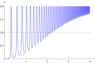
Figure 5: The $\displaystyle\epsilon(t)$ versus $\displaystyle t$ for $\displaystyle k=10^{6}$, $\displaystyle\omega=2$, $\displaystyle\alpha_{1}=10$,$\displaystyle\alpha_{2}=0$,$\displaystyle\alpha_{3}=2$. Compare with the figures in Sheikh

.

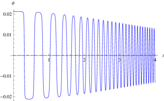
Figure 6: The $\displaystyle\psi_{-}$ versus $\displaystyle t$ with the same parameters as in Fig. 1 and $\displaystyle\beta=g=10^{-6}$. Compare with the figures in Sheikh

.

for $\displaystyle t>1$, the other terms, ($\displaystyle\alpha_{2},\cdots$), in (17) are important, and $\displaystyle f_{MS}(t)$ oscillates faster, so $\displaystyle\epsilon(t)$ and $\displaystyle\psi_{\pm}$ oscillate faster.
Finally, for $\displaystyle t\gg 1$, the denominator in (17) is increased, and results in $\displaystyle f_{MS}\approx 0$. Therefore in this regime, $\displaystyle\epsilon(t)\to 2$, $\displaystyle\psi_{-}\to 0$ as indicated in Fig. 5 and Fig. 6. Also, using (16), we have

$$H_{MS}(t)\to\frac{1}{2t}\hskip 2.168pt,\quad\psi_{+}\to\frac{1}{\sqrt{2}g}\frac{1}{t}$$ (25)

Results from various numerical analysis of the model with various initial values Sheikh have similar properties of the MS solutions, that lead us to the following conjecture about the model: the MS solution, (17), is the attractor solution of the model.

V Complementary slow roll conditions

If we demand that our fields be inflaton fields, complementary slow roll conditions are required in inflationary period ,i.e., not only $\displaystyle\epsilon(t)\ll 1$ but also

$$\delta_{\pm f}\equiv-\frac{\dot{\psi}_{\pm f}}{H_{f}\psi_{\pm f}}\ll 1\qquad,\hskip 21.68121pt\frac{\dot{\delta}_{\pm f}}{H_{f}\delta_{\pm f}}\ll 1.$$ (26)

For $\displaystyle\psi_{+f}$, the conditions do not have any restriction on the parameters of $\displaystyle\psi_{+f}$, therefore we will focus on $\displaystyle\psi_{-f}$.

V.1 Complementary slow roll conditions for the simple ansatz

For the simple ansatz, (8), the conditions in (26) yield

$$\frac{\omega}{H}\ll 2\tan\omega t_{inf}\qquad,\hskip 21.68121pt\frac{\omega}{H}\ll\frac{\sin 2\omega t_{inf}}{2}.$$ (27)

If $\displaystyle 0<\omega t_{inf}<{\pi}/{2}$, the conditions in (27) are reduced to $\displaystyle{\omega}\ll{H}$, that is agreement with (13).
If we take $\displaystyle\omega\Delta t_{inf}={1}/{2}$, then using the condition $\displaystyle{\omega}\ll{H}$, we obtain

$$H\Delta t_{inf}\gg 1.$$ (28)

The current cosmic microwave background data indicate that during inflation epoch, $\displaystyle H\lesssim 10^{-5}M_{pl}$ CMB-data . If $\displaystyle H\approx 10^{-5}M_{pl}$, the relation (28), implies that $\displaystyle\Delta t_{inf}\gg 10^{5}t_{pl}$.
Number of $\displaystyle e$-folding is given by

$$N_{e}=\int_{t_{i}}^{t_{f}}Hdt,$$ (29)

If we use $\displaystyle\omega\Delta t_{inf}={1}/{2}$, then assuming that $\displaystyle t_{f}>10t_{i}$, the numerical integration of the Hubble parameter in (11) shows that to have $\displaystyle N_{e}>60$, we must take $\displaystyle k>4\times 10^{6}$.
So, if we set $\displaystyle\beta=10^{-6}$ ( in Plank units), then to have sufficient $\displaystyle e$-folds, we must take $\displaystyle\kappa>2\times 10^{9}$.

V.2 Complementary slow roll conditions for the MS solution

As for the MS solutions, (26) yields

$$\begin{split}2(\alpha_{1}t\cot(\alpha_{1}t)-1)&\ll H_{MS}\hskip 2.168ptt\hskip 2.168pt,\cr\frac{1-(\alpha_{1}t\csc\alpha_{1}t)^{2}}{-1+\alpha_{1}t\cot\alpha_{1}t}~{}&\ll H_{MS}\hskip 2.168ptt\,.\end{split}$$ (30)

Here we have neglected other terms that do not have any effect in inflation period. For $\displaystyle\alpha_{1}t<1$ we have

$$\begin{split}2(\alpha_{1}t\cot(\alpha_{1}t)-1)&\approx-\frac{2(\alpha_{1}t)^{2}}{3}\hskip 2.168pt,\cr\frac{1-(\alpha_{1}t\csc\alpha_{1}t)^{2}}{-1+\alpha_{1}t\cot\alpha_{1}t}~{}&\approx 1+\frac{2}{15}(\alpha_{1}t)^{2})\,.\end{split}$$ (31)

Using Eqs. (20), (30) and (31), the complementary slow roll conditions are reduced to

$$\frac{k}{2(\sqrt{1+2k}-1)}\gg 1,$$ (32)

hence, it is sufficient that $\displaystyle k>8\times 10^{4}$.
Just like the simple ansatz, if we take $\displaystyle\alpha_{1}\triangle t_{inf}=1/2$, from relations (30) and (31), we have $\displaystyle H\triangle t_{inf}\gg 1$.
Number of $\displaystyle e$-folding is given by (20) and (29) as

$$N_{e}\approx\frac{k}{2(\sqrt{1+2k}-1)}\ln\frac{t_{f}}{t_{i}},$$ (33)

so, for $\displaystyle k>8\times 10^{4}$ we have

$$N_{e}>100\ln\frac{t_{f}}{t_{i}},$$ (34)

The general cosmological perturbation of the model was developed in Sheikh .

VI Reheating

In the most models for inflation to have successful reheating period, it is necessary that after inflation period, inflaton(s) behaves like dust matters, and then decays into relativistic matter. But in the Gauge-flation model the fields can be decayed into relativistic matter, without going to dust matter phase as we saw in §IV. One way to see this point is to see the Lagrangian (1), in the inflationary period the $\displaystyle(F\tilde{F})^{2}$ term is dominate, but after inflation this term is irrelevant, and the second term in (1) is dominate after inflation. Therefore the energy stored in fields are to be transferred to other fields by thermal bath of fields.
But if we demand that the energy density at the beginning of radiation epoch is the same as at the end of inflation, the thermal bath is not sufficient, due to the expansion of universe. So, a coupling between fields and matter is needed.
We suppose that the fields decay into relativistic particles, $\displaystyle\chi$, with decay rate, $\displaystyle\Gamma$, which depends on details of interactions between the fields with the relativistic particles. Here, we will obtain a bound on $\displaystyle\Gamma$ from conservation of energy. We have Weinberg

$$\begin{split}&\dot{\rho}_{\psi_{\pm}}+3H(\rho_{\psi_{\pm}}+p_{\psi_{\pm}})=-\Gamma\rho_{\psi_{\pm}},\cr&\dot{\rho}_{\chi}+3H(\rho_{\chi}+p_{\chi})=\Gamma\rho_{\psi_{\pm}}.\end{split}$$ (35)

Here

$$p_{\chi}/\rho_{\chi}=1/3,\hskip 21.68121ptp_{\psi_{-}}/\rho_{\psi_{-}}\equiv w_{eff}=-1+\frac{2}{3}\epsilon(t),$$ (36)

where $\displaystyle w_{eff}$ is the equation of state. Hence, we can solve (35) as

$$\rho_{\chi}=\frac{\rho_{\psi_{\pm}}(t_{r})}{a^{4}(t)}\frac{\Gamma M^{2}}{\omega H^{2}(t_{r})}\int_{\omega t_{r}}^{\omega t}a^{4}(\frac{\tau}{\omega})H^{2}(\frac{\tau}{\omega})e^{{\frac{\Gamma}{\omega}}(\tau_{r}-\tau)}\,\mathrm{d}\tau,$$ (37)

where $\displaystyle t_{r}$ is the time just after the end of inflation and $\displaystyle M$ is the scale energy of $\displaystyle H(t)$ that we explicitly show. After short time $\displaystyle H\rightarrow 1/2t$, and $\displaystyle a(t)\rightarrow a_{0}t^{\frac{1}{2}}$. By assuming that $\displaystyle\Gamma\gg\omega$, the fields almost immediately decay into $\displaystyle\chi$, i.e. $\displaystyle H(t_{r})\approx M$, so

$$\rho_{\chi}\approx\rho_{\psi_{\pm}(t_{r})}\left(\frac{a_{o}(t_{r})}{a(t)}\right)^{4}.$$ (38)

Therefore, to have successful inflation and reheating with this scenario, we need $\displaystyle H\Delta t_{inf}\gg 1$ and $\displaystyle\Gamma\Delta t_{inf}\gg 1$, one can set $\displaystyle\Gamma\approx H$. For the standard scalar field, to produce a successful radiation epoch after reheating period, we must take $\displaystyle\Gamma\gg H$ Weinberg .

VII Summary

We have studied the Gauge-flation by analytic methods and we have investigated the simple (but nontrivial) ansatz that shows the main features of the model. Then, we have derived formulas for leading order of fields in the model. The formulas are valid in all range of history of the early universe.
Using the formulas, we have provided analytic solutions for the MS solutions Sheikh , and with the analytic solutions, we studied some features of the MS solutions which cannot be obtained without analytic methods. Then, we obtained constraints from slow roll conditions on the parameters of the solutions.
Moreover, we studied preheating period in the model and obtained a bound on decay rate of fields, that may be useful for future works.

Appendix A

In this letter we give some solutions for Eq. (6), It is necessary to show that they are also solutions of the equation of motion for fields. To show this point, in this appendix we will obtain the equation of motion for fields in terms of variables that we use in this letter.
The equation of motion can be obtained by variation of (1) with respect to the fields as Sheikh

$$(1+\kappa g^{2}\frac{\phi^{4}}{a^{4}})\frac{\ddot{\phi}}{a}+(1+\kappa\frac{\dot{\phi}^{2}}{a^{2}})2g^{2}\frac{\phi^{3}}{a^{3}}+(1-3\kappa g^{2}\frac{\phi^{4}}{a^{4}})H\frac{\dot{\phi}}{a}=0.$$ (39)

But, another standard way, that we use here, to obtain (39) is to use the Friedman equations. For what we will do, let us review this method.
From (4), we obtain the following equations

$$H^{2}=\frac{1}{2}\left(\frac{\dot{\phi}^{2}}{a^{2}}+\frac{g^{2}\phi^{4}}{a^{4}}+\kappa^{2}\frac{g^{2}\phi^{4}\dot{\phi}^{2}}{a^{6}}\right),$$ (40)

and

$$\dot{H}=-(\frac{\dot{\phi}^{2}}{a^{2}}+\frac{g^{2}\phi^{4}}{a^{4}}).$$ (41)

the derivative of (40) with respect to time results in

$$2H\dot{H}=\frac{1}{2}\frac{d}{dt}\left(\frac{\dot{\phi}^{2}}{a^{2}}+\frac{g^{2}\phi^{4}}{a^{4}}+\kappa^{2}\frac{g^{2}\phi^{4}\dot{\phi}^{2}}{a^{6}}\right).$$ (42)

Substituting Eq. (41) into the left hand side of (42), with algebraic manipulations, gives us (39).
One way to obtain the equation of motion in terms of variables that we use in this letter, is to substitute variables in Eq. (39), but it is better to rewrite Eqs. (40) and (41) in terms of our variables, and then to derive the equation of motion.
For Eq. (40), we have

$$H^{2}=\frac{H^{2}}{2}\left(\epsilon(t)+\frac{\kappa^{2}}{4}\epsilon^{2}(t)H^{2}\sin^{2}2\alpha(t)\right),$$ (43)

and for Eq. (41), we have

$$\dot{H}=-\epsilon(t)H^{2}.$$ (44)

The derivative of (43) with respect to time, substituting Eq. (44) into the left hand side of the result, is

$$\begin{split}-2H^{3}\epsilon(t)&=H\dot{H}\left(\epsilon(t)+\frac{\kappa^{2}}{4}\epsilon^{2}(t)H^{2}\sin^{2}2\alpha(t)\right)\cr&+\frac{1}{2}H^{2}\frac{d}{dt}\left(\epsilon(t)+\frac{\kappa^{2}}{4}\epsilon^{2}(t)H^{2}\sin^{2}2\alpha(t)\right).\end{split}$$ (45)

We rearrange Eq. (45) as

$$\begin{split}0&=-\epsilon(t)H^{3}\left(-2+\epsilon(t)+\frac{\kappa^{2}}{4}\epsilon^{2}(t)H^{2}\sin^{2}2\alpha(t)\right)\cr&+\frac{1}{2}H^{2}\frac{d}{dt}\left(\epsilon(t)+\frac{\kappa^{2}}{4}\epsilon^{2}(t)H^{2}\sin^{2}2\alpha(t)\right).\end{split}$$ (46)

Eq. (46) is the equation of motion of fields in terms of our variables.
If we rewrite Eq. (6) as

$$\epsilon(t)+\frac{\kappa^{2}}{4}\epsilon^{2}(t)H^{2}\sin^{2}2\alpha(t)-2=0,$$ (47)

then, from Eqs. (46) and (47), we have

$$-\epsilon(t)H\left(L.H.S.\eqref{apreduced}\right)+\frac{1}{2}\frac{d}{dt}\left(L.H.S.\eqref{apreduced}\right)=0.$$ (48)

Therefore, solutions of Eq. (47) are the solutions of Eq. (48)

References

- (1) S. Weinberg, “Cosmology,” Oxford Univ. Press, Oxford, UK, 2008.
- (2) B. Ratra, Phys. Rev. D 45, 1913 (1992); L. F. Abbott, M. B. Wise, Nucl. Phys. B 244, 541 (1985).
- (3) A. Maleknejad, M. M. Sheikh-Jabbari, Phys. Rev. D 84, 043515 (2011); A. Maleknejad, M. M. Sheikh-Jabbari, [arXiv:1102.1513 [hep-ph]].
- (4) M. M. Sheikh-Jabbari, [arXiv:1203.2265[hep-th]].
- (5) P. Adshead, M. Wyman, Phys. Rev. Lett. 108, 261302 (2012)
- (6) M. Abramowitz, I. A. Stegun “Handbook of Mathematical Functions,”New York: Dover Publications. (1965).
- (7) E. Komatsu et al. [ WMAP Collaboration ], [arXiv:1001.4538 [astro-ph.CO]].