Magneto-Josephson effects in junctions with Majorana bound states

Abstract

We investigate 1D quantum systems that support Majorana bound states at interfaces between topologically distinct regions. In particular, we show that there exists a duality between particle-hole and spin degrees of freedom in certain spin-orbit-coupled 1D platforms such as topological insulator edges. This duality results in a spin analogue of previously explored ‘fractional Josephson effects’—that is, the spin current flowing across a magnetic junction exhibits $4\pi$ periodicity in the relative magnetic field angle across the junction. Furthermore, the interplay between the particle-hole and spin degrees of freedom results in unconventional magneto-Josephson effects, such that the Josephson current is a function of the magnetic field orientation with periodicity $4\pi$.

The possibility of observing Majorana zero-modes in condensed matter has captured a great deal of attention in recent years. Much effort in this pursuit presently focuses on spin-orbit-coupled 1D wires, which are closely related to edges of 2D topological insulators (TIs). In either setting Majorana modes are predicted to localize through the competition between superconducting proximity effects and Zeeman splitting Fu and Kane (2009); Lutchyn et al. (2010); Oreg et al. (2010); Jiang et al. (2011); Beenakker (2011); Alicea (2012). Remarkably, zero-bias conductance anomalies Sengupta et al. (2001); Bolech and Demler (2007); Law et al. (2009); Flensberg (2010); Fidkowski et al. (2012) possibly originating from Majorana modes have even been measured Mourik et al. (2012); Das et al. (2012) very recently in quantum wires. Numerous other fascinating phenomena tied to Majorana fermions have also been explored, including non-Abelian statistics Read and Green (2000); Ivanov (2001); Alicea et al. (2011), electron teleporation Fu (2010), and exotic Josephson effects Kitaev (2001); Fu and Kane (2009); Jiang et al. (2011).

Particularly interesting to us here are the Majorana-related Josephson effects in quantum wires and TI edges. Consider two Majorana modes hybridized across a Josephson junction formed by topological superconducting regions separated by a narrow barrier as shown in Fig. 1(b). The energy splitting of these Majoranas depends periodically on half the phase difference between the right and left superconductors, $(\phi_{r}-\phi_{l})/2$, giving rise to a Josephson current with $4\pi$ periodicity in $\phi_{r}-\phi_{l}$ Kitaev (2001); Fu and Kane (2009). If, in addition, a third superconductor contacts the middle domain, a difference between its phase and the average phase $(\phi_{r}+\phi_{l})/2$ induces a non-local three-leg “zipper” Josephson current that divides equally between the two leads and is also $4\pi$ periodic in $\phi_{r}$ and $\phi_{l}$ Jiang et al. (2011). These ‘fractional Josephson effects’ provide smoking-gun signatures of Majorana modes.

Our claim is that physical quantities of Majorana junctions in wires and TI edges can also possess $4\pi$-periodic dependence on the orientations of Zeeman fields applied in the plane normal to the spin orbit direction. Notably, in some domain configurations the Majorana-mediated Josephson current reverses sign after a full $2\pi$ rotation of the magnetic field orientation on one side of the junction. Only an additional $2\pi$ rotation restores the currents to their original direction. Thus the mixing between the particle-hole and spin degrees of freedom leads to an unconventional magneto-Josephson effect through the coupling of Majoranas.

Additionally, the Majorana modes produce a ‘spin Josephson current’ between the magnets providing the Zeeman energy, which could also be $4\pi$ periodic in the field orientations. Define $\theta_{s}$ as the angle between the wire and the Zeeman field at domain $s$. Spin Josephson currents, $j^{S}$, are equivalent to torques (driven partly by the Majoranas) that the wire domains apply on the external magnets . Therefore, they are given by the derivative of the system’s energy with respect to the magnetic field orientations $\theta$:

$$j^{S}=\frac{\partial\left\langle{\mathcal{H}}\right\rangle}{\partial\theta}.$$ (1)

with $\mathcal{H}$ being the system’s Hamiltonian. In the case of TI edges, the spin currents arise as the exact duals of Josephson currents, and the orientation of the B-field is the exact dual to the superconducting phase (indeed, the Josephson current is given by $j^{Q}=\frac{2e}{\hbar}\frac{\partial\left\langle{\mathcal{H}}\right\rangle}{\partial\phi}$). We emphasize that the $4\pi$ periodicity prevails as long as the parity of the Majorana state remains constant during the measurement, or changes at a slower rate than the winding of the superconducting phase and magnetic orientations.

Let us focus first on the analysis of the $4\pi$-periodic orientation dependence in TI edges, before commenting on spin-orbit-coupled wires which obey qualitatively similar rules. The Hamiltonian, including s-wave pairing and Zeeman fields in both the transverse and parallel directions relative to the spin-orbit direction, reads

$${\mathcal{H}}=v\hat{p}\tau^{z}\sigma^{z} -\mu\tau^{z}+\Delta\left(\cos\phi~{}\tau^{x}-\sin\phi~{}\tau^{y}\right)$$

$$-b\sigma^{z}+B\left(\cos\theta~{}\sigma^{x}-\sin\theta~{}\sigma^{y}\right).$$ (2)

Here we have employed the Nambu spinor basis $\Psi^{T}=(\psi_{\uparrow},\psi_{\downarrow},\psi_{\downarrow}^{\dagger},-\psi_{\uparrow}^{\dagger})$ and introduced Pauli matrices $\sigma^{a}$ and $\tau^{a}$ that act in the spin and particle-hole sectors, respectively. The edge-state velocity is given by $v$, $\hat{p}$ is the momentum, and the $\sigma^{z}$-direction represents the spin-orbit-coupling axis. We allow the chemical potential $\mu$, superconducting pairing $\Delta e^{i\phi}$, longitudinal magnetic field strength $b$, transverse magnetic field strength $B$, and the transverse-field orientation angle $\theta$ to vary spatially. Interestingly, Eq. (2) has a magnetism-superconductivity duality—the Hamiltonian takes the same form upon interchanging the magnetic terms $\left\{b,B,\theta,\sigma^{a}\right\}$ with the superconducting terms $\left\{\mu,\Delta,\phi,\tau^{a}\right\}$. Below we deduce the physical consequences of this duality.

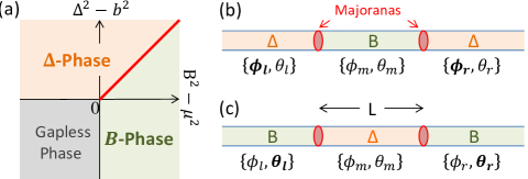
Figure 1: (a) Phase diagram for 1D system: gapless-phase ($B^{2}\leq\mu^{2}$ and $\Delta^{2}\leq b^{2})$, $\mathrm{\Delta}$-phase ($\Delta^{2}-b^{2}>\max\left[B^{2}-\mu^{2},0\right]$), and B-phase ($B^{2}-\mu^{2}>\max\left[\Delta^{2}-b^{2},0\right]$). Both $\mathrm{\Delta}$-phase and B-phase are gapped. (b) The $\mathrm{\Delta}$-B-$\mathrm{\Delta}$ junction supports Majorana bound states at the domain walls Jiang et al. (2011). (c) The dual configuration of B-$\mathrm{\Delta}$-B junction that also supports Majoranas.

The Hamiltonian (2) supports three different phases determined by the relative strength of $\left\{\Delta,\mu,B,b\right\}$. As Fig. 1(a) illustrates, we have (i) a topological superconducting gapped phase (denoted henceforth as the $\mathrm{\Delta}$-phase) when $\Delta^{2}-b^{2}>\max\left[B^{2}-\mu^{2},0\right]$, (ii) a topological magnetic gapped phase (denoted B-phase) when $B^{2}-\mu^{2}>\max\left[\Delta^{2}-b^{2},0\right]$, and (iii) a trivial gapless state when $B^{2}\leq\mu^{2}$ and $\Delta^{2}\leq b^{2}$. Consistent with the magnetic-superconducting duality, in the phase diagram of Fig. 1(a) the B- and $\mathrm{\Delta}$-phases are symmetrically arranged with respect to the diagonal line that defines the boundary between these two gapped states:

$$\Delta^{2}+\mu^{2}=B^{2}+b^{2}.$$ (3)

Majorana zero-modes bind to domain walls separating B- and $\mathrm{\Delta}$-domains. For notational simplicity, below we will assume that $\Delta>b>0$ and $B>\mu>0$, though more general results can be obtained App . We will also focus on setups for which all domains experience both superconductivity and a transverse Zeeman field.

In TI edges, the $4\pi$ periodic dependence on the magnetic field orientation occurs when two Majoranas are nestled in a $\mathrm{B-\Delta-B}$ domain sequence as in Fig. 1(c). This is in contrast to the previously studied unconventional Josephson effects Kitaev (2001); Fu and Kane (2009); Jiang et al. (2011), which occur over a junction between two $\mathrm{\Delta}$-domains bridged by a B-domain [see Fig. 1(b)]. The magneto-Josephson and spin-Josephson effects of a TI edge follow from the detailed dependence of the Majorana energy splitting, ${E_{\mathrm{Maj}}}$, on the field orientations and superconducting phases in the $\mathrm{B-\Delta-B}$ edge domain structure of Fig. 1(c). In addition to an exact numerical calculation of ${E_{\mathrm{Maj}}}$, we provide in App an analytical variational approach that sheds light on the physics. In the latter approach we assume that the Majorana wavefunctions are unmodified by their proximity to each other, apart from being superposed to form a conventional low-lying state. This leads to an energy splitting that is suppressed as a weighted sum of two exponentials which control the decay of the Majorana wave functions in the middle domain.

Our results for the Majorana couplings constitute one of the central results of this paper. The two characteristic decay lengths as a function of field and pairing are $\lambda_{1,2}=\frac{v}{|\sqrt{\Delta^{2}-b^{2}}\pm\sqrt{B^{2}-\mu^{2}}|}$. Quite generally, for the middle $\mathrm{\Delta}$-domain of length $L$, the Majorana coupling energy is:

$$\frac{E_{\mathrm{Maj}}}{E_{0}\left[\delta\phi_{l,r}\right]} \approx e^{-\lambda_{m,1}L}\sin\frac{\delta\theta_{l}-\tilde{\mu}_{m}+\tilde{\mu}_{l}}{2}\sin\frac{\delta\theta_{r}+\tilde{\mu}_{m}-\tilde{\mu}_{r}}{2}$$

$$-e^{-\lambda_{m,2}L}\sin\frac{\delta\theta_{l}+\tilde{\mu}_{m}+\tilde{\mu}_{l}}{2}\sin\frac{\delta\theta_{r}-\tilde{\mu}_{m}-\tilde{\mu}_{r}}{2}.$$ (4)

Here we have defined $\delta\phi_{\ell,r}\equiv\phi_{\ell,r}-\phi_{m}$, $\delta\theta_{\ell,r}\equiv\theta_{\ell,r}-\theta_{m}$, $\tilde{\mu}_{l/m/r}\equiv\cos^{-1}\frac{\mu_{l/m/r}}{B_{l/m/r}}$, $\tilde{b}_{l/m/r}\equiv\cos^{-1}\frac{b_{l/m/r}}{\Delta_{l/m/r}}$, along with a characteristic energy

$$E_{0}\left[\delta\phi_{l,r}\right]=\frac{\sin\tilde{b}_{m}}{\sin\tilde{\mu}_{m}}\frac{1}{\sqrt{M_{l}\left[\delta\phi_{l}\right]M_{r}\left[\delta\phi_{r}\right]}}.$$ (5)

The denominator of $E_{0}$ follows from

$$M_{s} \left[\delta\phi_{s}\right]\approx\left.\begin{array}[c]{c}\frac{\left(\Delta_{m}^{2}+\mu_{m}^{2}-b_{m}^{2}\right)}{2\sqrt{\Delta_{m}^{2}-b_{m}^{2}}\left(\Delta_{m}^{2}+\mu_{m}^{2}-B_{m}^{2}-b_{m}^{2}\right)}\\ \end{array}\right.$$ (7)

$$\left.\begin{array}[c]{c}+\frac{\left(B_{s}^{2}+b_{s}^{2}-\mu_{s}^{2}\right)+\Delta_{s}\left[\sqrt{B_{s}^{2}-\mu_{s}^{2}}\sin\left(\tilde{b}_{m}\pm\delta\phi_{s}\right)-b_{s}\cos\left(\tilde{b}_{m}\pm\delta\phi_{s}\right)\right]}{2\sqrt{B_{s}^{2}-\mu_{s}^{2}}\left(B_{s}^{2}+b_{s}^{2}-\Delta_{s}^{2}-\mu_{s}^{2}\right)},\\ \end{array}\right.$$ (9)

with the choice of sign $\pm$ depending on $s=l$ or $r$. Note that $M_{s}$ exhibits the standard $2\pi$ periodicity in $\phi_{s}$, so that the more exotic $4\pi$ periodicity follows exclusively from the trigonometric functions in Eq. (4).

These general results allow us to quantitatively estimate the magneto-Josephson effects described earlier, which can be measured in the circuit sketched in Fig. 2(a). For simplicity, we specialize to the case of $\mu_{l/m/r}=0$, where the Majorana coupling energy reduces to

$$E_{\mathrm{Maj}}\approx\epsilon_{M}[\delta\phi_{\ell,r}]\cos\frac{\theta_{l}-\theta_{r}}{2}+\epsilon_{Z}[\delta\phi_{\ell,r}]\cos\frac{\theta_{l}+\theta_{r}-2\theta_{m}}{2},$$ (10)

with $\epsilon_{M/Z}[\delta\phi_{\ell,r}]=E_{0}[\delta\phi_{\ell,r}]\frac{e^{-L/\lambda_{m,2}}\pm e^{-L/\lambda_{m,1}}}{2}$.

The Majorana-related magneto-Josephson currents entering the $s=\ell/r$ electrode are $j_{s}^{Q}=\frac{2e}{\hbar}\frac{\partial\left\langle{\mathcal{H}}\right\rangle}{\partial\phi_{s}}=p\frac{2e}{\hbar}\frac{E_{\mathrm{Maj}}}{\partial\phi_{s}}$, where $p=\pm 1$ denotes the parity of the hybridized Majoranas. The explicit form for the charge currents (dropping the parity factor $p$) is:

$$\begin{array}[c]{c}j_{\ell/r}^{Q}\approx\pm j_{M}^{Q}\cos\frac{\theta_{l}-\theta_{r}}{2}+j_{Z}^{Q}\cos\frac{\theta_{l}+\theta_{r}-2\theta_{m}}{2},\\ \text{{with:}}\mathrm{\,\,\,}j_{M/Z}^{Q}=\frac{2e}{\hbar}\frac{\partial\epsilon_{M/Z}}{\partial\phi_{\ell/r}}.\end{array}$$ (11)

which constitutes a prediction for the unconventional magneto-Josephson effect. The analytical expressions obtained above for $j_{M}^{Q}$ and $j_{Z}^{Q}$ agree well with the numerical calculations for large $L$ as shown in Fig. 2(b). They confirm that for B-$\mathrm{\Delta}$-B junctions the Majorana coupling induces the charge current $j_{l/r}^{Q}$ with $4\pi$ periodic dependence on $\theta_{l/r}$.

Similarly the spin Josephson currents, or torques on the magnets, in region $s=\ell/r$ are $j_{s}^{S}=-\frac{\partial\left\langle{\mathcal{H}}\right\rangle}{\partial\theta_{s}}=p\frac{\partial E_{\mathrm{Maj}}}{\partial\theta_{s}}$ [Eq. (1)]. The angular momentum transferred by these currents is in the direction parallel to the spin-orbit axis, which in this case is the $z$-direction. The spin Josephson currents are thus given by:

$$\begin{array}[c]{c}j_{l/r}^{S}=\pm j_{M}^{S}\sin\frac{\theta_{l}-\theta_{r}}{2}+j_{Z}^{S}\sin\frac{\theta_{l}+\theta_{r}-2\theta_{m}}{2},\\ \text{{with:}}\mathrm{\,\,\,}j_{M/Z}^{S}=\frac{\epsilon_{M/Z}}{2}.\end{array}$$ (12)

The $j_{M}^{S}$ spin current exchanges angular momentum between the right and left magnets directly, while the $j_{Z}^{S}$ spin current originates in the middle region and equally splits into the right and left regions, $j_{m\rightarrow l}^{S}=j_{m\rightarrow r}^{S}=j_{Z}^{S}\sin\frac{\theta_{l}+\theta_{r}-2\theta_{m}}{2}$. This term vanishes when there is no transverse magnetic field in the middle domain, and represents the dual of the zipper Josephson effect in the $\mathrm{\Delta}$-B-$\mathrm{\Delta}$ junction that splits charge current from the middle domain between the two side domains Jiang et al. (2011).

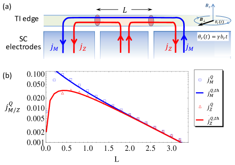
Figure 2: (a) The scheme to measure unconventional magneto-Josephson effect. Josephson currents are measured for the B-$\mathrm{\Delta}$-B junction. In the right region, the transverse magnetic field winds at rate $\omega_{L}=\gamma b_{r}$, which modulates the Josephson current at half the frequency, $\omega_{L}/2$. (b) Comparison between analytical expressions and numerical results for $j_{M}$ and $j_{Z}$. The parameters are $\mu_{l/m/r}=0$, $b_{l/m/r}=1/2$, $\Delta_{m}=2.5$, $\Delta_{l/r}=1$, $B_{l/r}=2$, $B_{m}=1$. The superconducting angles are fixed $\phi_{l/r}=\pi/2$, $\phi_{m}=0$.

The origin of this exotic dependence of the Majorana-related currents can be traced to the magnetic-superconducting duality in topological insulator edges Fu and Kane (2009); Jiang et al. (2011). For a junction with three alternating domains, there are two dual configurations: the $\mathrm{\Delta}$-B-$\mathrm{\Delta}$ junction [Fig. 1(b)] and the B-$\mathrm{\Delta}$-B junction [Fig. 1(c)]. The spin-Josephson effect in the B-$\mathrm{\Delta}$-B junction is dual to the charge-Josephson effect in the $\mathrm{\Delta}$-B-$\mathrm{\Delta}$ junction Fu and Kane (2009); Lutchyn et al. (2010); Oreg et al. (2010); Jiang et al. (2011). Similarly, the magneto-Josephson effect depending on the orientation angles in the B-$\mathrm{\Delta}$-B junction has a dual spin-Josephson effect depending on the superconducting angles in the $\mathrm{\Delta}$-B-$\mathrm{\Delta}$ junction.

Majorana junctions in spin-orbit coupled wires exhibit the same magneto-Josephson and spin-Josephson effects as the TI edge. The wire’s Hamiltonian adds a kinetic energy piece to Eq. (2), $\mathcal{H}_{k}=\frac{1}{2m}{\hat{p}}^{2}\tau^{z}$. This produces additional Fermi points at ‘large’ momenta $p_{F}\sim\pm 2mv$ that are, however, nearly unaffected by the magnetic field in the presence of pairing. Therefore the analysis above for the TI edges still applies qualitatively. Thus, in a Majorana wire, $4\pi$-periodic effects in both $\theta$ and $\phi$ appear in the $B-\Delta-B$ domain sequence . The quantitative analysis of the magneto-, spin-, and charge-Josephson effects in wires as well as the role of Andreev bound states will be analyzed elsewhere InP .

Observing the unconventional magneto-Josephson effect and the $4\pi$ periodicity in $\theta_{l/r}$ [see Fig. 3(b)] requires effective control of the magnetic field orientation. In particular, the orientation change needs to be sufficiently fast so that the Majorana states’ total parity does not change, but still slow on the scale of the inverse bulk gap to avoid quasiparticle poisoning San-Jose et al. (2011). The rate of parity decay is strongly detail dependent, but we surmise that measurements with rates faster than $1$ kHz and slower than the minimum gap in the device would suffice. Conventional magnets may be too unwieldy when made to rapidly turn; nuclear magnetization, however, could be ideal for this task. Through the hyperfine coupling, a polarized nuclear spin population could create an effective Zeeman field in the plane perpendicular to the spin-orbit coupling direction. For example, large nuclear spin polarization, normal to the spin-orbit direction, can be induced by optical pumping with circularly polarized light Kikkawa and Awschalom (2000). An external magnetic field with strength $b$, applied parallel to the spin-orbit axis, would make the orientation angle of the hyperfine transverse field wind at a rate $\omega_{L}=\gamma b$, where $\gamma/2\pi\approx-7.6$ MHz/T for ¹⁹⁹Hg or $\gamma/2\pi\approx 13.5\$MHz/T for ¹²⁵Te nuclei Willig et al. (1976). The hyperfine transverse field can be rather strong, e.g., $B\sim 0.1$ Tesla for $2\%$ nuclear polarization fraction Kikkawa and Awschalom (2000). It can, moreover, persist for long times, limited by the inhomogeneous nuclear transverse spin lifetime $T_{2}^{\ast}\sim 100$ $\mu$s, which already suffices for hundreds of precession periods for $b\sim 0.1$ Tesla. The transverse spin lifetime can be further extended using spin echo techniques.

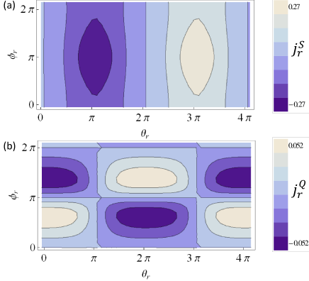
Figure 3: Contour plot of (a) spin current $j_{r}^{S}$ and (b) charge current $j_{r}^{Q}$, both of which are $4\pi$ periodic in $\theta_{r}$ and $2\pi$ periodic in $\phi_{r}$. The other angles are fixed $\phi_{l}=\pi/2$, $\phi_{m}=\theta_{l/m}=0$. The parameters are the same as Fig. 2.

With a rotating transverse magnetic field, we can observe the magneto-Josephson effect in several ways. A constantly winding orientation in the left domain, $\theta_{r}\left(t\right)=\omega_{L}t$ [while fixing $\theta_{l/m}\left(t\right)=0$, as illustrated in Fig. 2(a)], produces an oscillatory component of the charge current with amplitude $j_{\omega_{L}/2}^{Q}=j_{M}^{Q}+j_{Z}^{Q}=\frac{2e}{\hbar}\frac{\partial E_{0}}{\partial\phi}e^{-L/\lambda_{m-}}$ at half the frequency, $\omega_{L}/2$. In TI edges, we can also use resonant properties to probe the orientation-frequency halving. A DC voltage $V$ applied to the right superconducting lead, for instance, induces a winding of the superconducting angles, $\phi_{r}\left(t\right)=2eVt/\hbar$ and $\phi_{l/m}\left(t\right)=0$. When the magnetic orientation also winds with angular velocity $\Omega_{L}$, interference between the two oscillation would yield a DC current from the right superconducting lead, when $\omega_{L}=2\Omega_{V}$ (neglecting high-order resonances). The amplitude of the dc current is expected to be:

$$j_{\omega_{L}=2\Omega_{V}}^{Q,DC}\approx\frac{1}{2\pi}\int_{0}^{2\pi}j_{\omega_{L}/2}^{Q}\left[\phi_{r}\right]\cos\phi_{r}d\phi_{r}.$$ (13)

Alternatively, one can apply an AC voltage to the right superconducting lead such that $\phi_{r}\propto\sin\omega t$, while all other superconducting angles are held fixed. Interference effects now produce Shapiro-step-like resonant features which emerge only when

$$\omega_{L}=2n\omega$$ (14)

for even integer $2n$ (neglecting higher order corrections to the $\theta$ dependence).

The Majorana-mediated spin currents with $4\pi$ phase periodicity are harder to measure. A possible route for such measurements is to use a magnetic nanoparticle as the magnetic field source on one of the side domains. The torques on the nanoparticle could be probed from the shift in the ferromagnetic resonance (FMR) frequency. The FMR frequency is typically $f_{0}\sim 10$ GHz. The FMR linewidth, dictated by the Gilbert damping coefficient $\alpha$, is of order $\alpha f_{0}=0.01f_{0}$ in bulk ferromagnets, but is probably much smaller in nanoparticles Cehovin et al. (2003). A rough estimate of the maximum Majorana-related spin-current (or torque), $j^{S}$, yields $j^{S}\sim\hbar\cdot 10$ GHz. This produces a frequency shift around $j^{S}/m_{total}$, which is inversely proportional to the total angular momentum of the FM grain $m_{total}$ Brataas et al. (2012). This shift must dominate the FMR linewidth, $j^{S}/m_{total}>f_{0}\alpha$. The nanograin must, therefore, be sufficiently small such that $m_{total}/\hbar<\alpha^{-1}\sim 100$, e.g. have a radius of around $10$ nm, and still provide a sufficient Zeeman field for the domain it is on.

Measuring the effect of the relative field orientation on the spin and charge currents can be complicated by the presence of conventional Josephson effects arising from the continuum states. Indeed, the bulk energy associated with the continuum states also has dependence on magnetic field orientations and superconducting phases that are interesting in their own right, and of similar magnitude to the Majorana related effects. Nonetheless, all these dependencies are $2\pi$ periodic, as we have confirmed numerically. Hence, the measurement schemes proposed above will be insensitive to them.

In conclusion, we explored consequences of a magnetism-superconductivity duality of TI edge states, emphasizing Josephson effects. Most prominently, the duality implies that spin and charge Josephson currents in TI edges exhibit a $4\pi$ periodic dependence on the orientation difference of the magnetic field. These remarkable effects are a direct consequence of the Majorana states and we make several proposals how to detect them experimentally. The duality is only approximate in spin-orbit-coupled quantum wires but analogous effects also occur in this system. In addition to the Josephson effects, the duality has further interesting implications. For instance, it implies that the transition between topological and trivial phases can be tuned using a magnetic gradient, which is the dual of the superconducting phase gradient Romito et al. (2012).

Note added:

As we are completing the manuscript we became aware of overlap work by Qinglei Meng, Vasudha Shivamoggi, Taylor Hughes, Matthew Gilbert, and Smitha Vishveshwara Meng et al. (2012).

It is a pleasure to thank M. P. A. Fisher, L. Glazman, A. Haim, B. Halperin, A. Kitaev, L. Kouwenhoven, C. Marcus, J. Meyer, Y. Most, F. Pientka, J. Preskill, X.L. Qi, K. Shtengel, and A. Stern for useful discussions, and the Aspen Center for Physics for hospitality. We are also grateful for support from the NSF through grant DMR-1055522, BSF, SPP1285 (DFG), NBRPC (973 program) 2011CBA00300, the Alfred P. Sloan Foundation, the Packard Foundation, the Humboldt Foundation, the Minerva Foundation, the Sherman Fairchild Foundation, the Lee A. DuBridge Foundation, the Moore-Foundation funded CEQS, and the Institute for Quantum Information and Matter (IQIM), an NSF Physics Frontiers Center with support of the Gordon and Betty Moore Foundation.

Appendix A Supplementary materials

We study the linearized 1D system

$$H\left(\mu,\Delta,\phi;b,B,\theta\right)=p\tau^{z}\sigma^{z}-\mu\tau^{z}+\Delta\left(\tau^{x}\cos\phi-\tau^{y}\sin\phi\right)-b\sigma^{z}+B\left(\sigma^{x}\cos\theta-\sigma^{y}\sin\theta\right)$$ (15)

with six control parameters: $\mu$ for the chemical potential, $\Delta$ for the pairing energy, $\phi$ for the superconducting phase, $-b$ for the longitudinal magnetic field, $B$ for the transversal magnetic field, and $\theta$ for angle of the transversal magnetic field. In this form, the duality between $\left(\Delta,\mu\right)$ and $\left(B,b\right)$ is more obvious. Without loss of generality, we assume that all the control parameters $\left(\mu,\Delta,b,B\right)$ are all positive.

A.1 Phase Diagram

We compute the determinant

$$\det H=\left[p^{2}+\left(\sqrt{B^{2}-\mu^{2}}+\sqrt{\Delta^{2}-b^{2}}\right)^{2}\right]\left[p^{2}+\left(\sqrt{B^{2}-\mu^{2}}-\sqrt{\Delta^{2}-b^{2}}\right)^{2}\right].$$ (16)

The energy gap will be closed if there exist some real solutions of $p$ to satisfy $\det H=0$.

1. When $B^{2}\leq\mu^{2}$ and $\Delta^{2}\leq b^{2}$, the system is in a gapless-phase, because there are real solutions $p=\pm\left(\sqrt{-B^{2}+\mu^{2}}+\sqrt{-\Delta^{2}+b^{2}}\right)$ or $p=\pm\left(\sqrt{-B^{2}+\mu^{2}}-\sqrt{-\Delta^{2}+b^{2}}\right)$ to fulfill the requirement of $\det H=0$.

2. When $B^{2}>\mu^{2}$ or $\Delta^{2}>b^{2}$, the system is always gapped, because there are no real solutions of $p$ to satisfy $\det H=0$.

   1. For $\Delta^{2}-b^{2}>\max\left[B^{2}-\mu^{2},0\right]$, the system is in a superconducting gapped phase ($\Delta$-phase).

   2. For $B^{2}-\mu^{2}>\max\left[\Delta^{2}-b^{2},0\right]$, the system is in a magnetic gapped phase ($B$-phase).

   3. There is a quantum phase transition at $\Delta^{2}-b^{2}=B^{2}-\mu^{2}$, which connects the $\Delta$-phase and the $B$-phase.

Therefore, we obtain the phase diagram in Fig. 1(a).

A.2 1D System Consisting of Different Regions

We are interested in the case that the 1D system consists of three regions of different control parameters. Specifically

$$\chi=\left\{\begin{tabular}[c]{ll}$\chi_{l}$&for $x\in\left(-\infty,0\right)$\\ $\chi_{m}$&for $x\in\left(0,L\right)$\\ $\chi_{r}$&for $x\in\left(L,+\infty\right)$\end{tabular}\right.$$ (17)

with $\chi$ representing the six control parameters. The system Hamiltonian is

$$H=\left\{\begin{tabular}[c]{ll}$H_{l}$&for $x\in\left(-\infty,0\right)$\\ $H_{m}$&for $x\in\left(0,L\right)$\\ $H_{r}$&for $x\in\left(L,+\infty\right)$\end{tabular}\right.$$ (18)

with $H_{f}\equiv H\left(\mu_{f},\Delta_{f},\phi_{f};b_{f},B_{f},\theta_{f}\right)$. We are interested in the $B-\Delta-B$ configuration, with $B_{l}^{2}-\mu_{l}^{2}>\max\left[\Delta_{l}^{2}-b_{l}^{2},0\right]$, $\Delta_{m}^{2}-b_{m}^{2}>\max\left[B_{m}^{2}-\mu_{m}^{2},0\right]$, and $B_{r}^{2}-\mu_{r}^{2}>\max\left[\Delta_{r}^{2}-b_{r}^{2},0\right]$.

A.3 Perturbative Formulism for the Coupling Energy

Let’s first consider the individual Majoranas. The left Majorana $\left|L\right\rangle$ is at $x=0$ associated with the $l-m$ boundary. We may introduce the Hamiltonian $H_{L}=\left\{\begin{tabular}[c]{ll}$H_{l}$&for $x\in\left(-\infty,0\right)$\\ $H_{m}$&for $x\in\left(0,\infty\right)$\end{tabular}\ \right.$ that supports the zero energy Majorana mode $\left|L\right\rangle$, with $H_{L}\left|L\right\rangle=0.$Similarly, the right Majorana $\left|R\right\rangle$ is at $x=L$ associated with the $m-r$ boundary. We can also introduce $H_{R}=\left\{\begin{tabular}[c]{ll}$H_{m}$&for $x\in\left(-\infty,L\right)$\\ $H_{r}$&for $x\in\left(L,+\infty\right)$\end{tabular}\ \right.$ that supports zero-energy Majorana mode $\left|R\right\rangle$, with $H_{R}\left|R\right\rangle=0.$ We can can perturbatively compute the coupling energy between $\left|L\right\rangle$ and $\left|R\right\rangle$ by the formula:

$${\mathcal{H}}_{LR}\approx M^{-1/2}hM^{-1/2}$$ (19)

with $M$ being the overlap matrix between the (not necessarily normalized) Majorana states, and $h$ being:

$$h=\left(\begin{array}[c]{cc}0&\left\langle L\right|\Delta V\left|R\right\rangle\\ \left\langle R\right|\Delta V\left|L\right\rangle&0\end{array}\right)$$ (20)

with:

$$\Delta V=H-H_{L}=\left(H_{r}-H_{m}\right)\eta\left(x-L\right).$$ (21)

Therefore, the coupling Hamiltonian is approximately ${\mathcal{H}}_{LR}\approx\left(\begin{array}[c]{cc}0&E\\ E^{\ast}&0\end{array}\right)$, with

$$E\approx\frac{\left\langle L\right|\Delta V_{L}\left|R\right\rangle}{\sqrt{\left\langle L|L\right\rangle\left\langle R|R\right\rangle}}.$$ (22)

A.4 Wavefunction of Individual Majoranas

We can rewrite the Hamiltonian as

$$H_{L} =H_{l}\eta\left(-x\right)+H_{m}\eta\left(x\right)$$ (23)

$$=\left\{\begin{tabular}[c]{ll}$U_{l}\cdot V\cdot\left(p-K_{l}\right)\cdot V^{{\dagger}}\cdot U_{l}^{{\dagger}}\tau^{z}\sigma^{z}$&for $x<0$\\ $U_{m}\cdot V\cdot\left(p-K_{m}\right)\cdot V^{{\dagger}}\cdot U_{m}^{{\dagger}}\tau^{z}\sigma^{z}$&for $x>0$\end{tabular}\ \ \ \right..$$ (26)

where the unitary transformations are

$$V=e^{-i\frac{\pi}{4}\tau^{z}\sigma^{z}}$$ (27)

$$U=e^{i\frac{\phi}{2}\tau^{z}}\otimes e^{i\frac{\theta}{2}\sigma^{z}}\equiv:U_{\phi}\otimes U_{\theta}$$ (28)

and the non-Hermitian matrix is

$$K=\left(b\tau^{z}+i\Delta\tau^{x}\right)+\left(\mu\sigma^{z}+iB\sigma^{x}\right)$$ (29)

with sub-index $f=l,m,r$ not explicitly written for simplicity. Without loss of generality, we can fix

$$\phi_{m}=\theta_{m}=0$$ (30)

and $U_{m}=I$. For our notational convenience, we also introduce $\tilde{b}\equiv\cos^{-1}\frac{b}{\Delta}$ and $\tilde{\mu}\equiv\cos^{-1}\frac{\mu}{B}$. (Let’s assume $\Delta^{2}>b^{2}$ and $B^{2}>\mu^{2}$ for notational simplicity. Later we will show that this constraint can be relaxed.) The eigensystem of $K$ is

$$K\cdot\left(v_{\tilde{b}}^{s_{1}}\otimes v_{\tilde{\mu}}^{s_{2}}\right)=\Lambda^{s_{1},s_{2}}\left(v_{\tilde{b}}^{s_{1}}\otimes v_{\tilde{\mu}}^{s_{2}}\right)$$ (31)

with sub-eigenvectors

$$\framebox{$v_{\xi}^{s}=\frac{1}{\sqrt{2}}\left(-ie^{is\xi/2},e^{-is\xi/2}\right)^{T}=v_{s\xi}^{+}$}$$ (32)

and eigenvalues

$$\framebox{$\Lambda^{s_{1},s_{2}}=\Delta~{}\lambda_{\tilde{b}}^{s_{1}}+B~{}\lambda_{\tilde{\mu}}^{s_{2}}$}$$ (33)

where

$$\lambda_{\xi}^{s}=\lambda_{s\xi}^{+}=i\sin s\xi$$ (34)

for $s=\pm 1$. $\left(v_{\xi}^{+}\right)^{T}\cdot v_{\xi^{\prime}}^{+}=-i\sin\frac{\xi+\xi^{\prime}}{2}$. The two-vectors $v_{\xi}^{s}=v_{s\xi}^{+}$ have the following properties of inner-products:

$$\left(v_{\xi}^{s}\right)^{T}\cdot v_{\xi}^{s^{\prime}}=-i\sin s\xi~{}\delta_{s,s^{\prime}}=\left(\begin{array}[c]{cc}-i\sin\xi&0\\ 0&i\sin\xi\end{array}\right)$$ (35)

$$\left(v_{\xi}^{s}\right)^{{\dagger}}\cdot\sigma^{z}\cdot v_{\xi}^{s^{\prime}}=-i\sin s\xi~{}\delta_{\bar{s},s^{\prime}}=\left(\begin{array}[c]{cc}0&-i\sin\xi\\ i\sin\xi&0\end{array}\right)$$ (36)

$$\left(v_{\xi}^{s}\right)^{{\dagger}}\cdot v_{\xi}^{s^{\prime}}=\delta_{s,s^{\prime}}+\cos\xi~{}\delta_{\bar{s},s^{\prime}}=\left(\begin{array}[c]{cc}1&\cos\xi\\ \cos\xi&1\end{array}\right)$$ (37)

where $\bar{s}:\equiv-s$ for $s=\pm 1$. And it transforms under the unitary

$$\framebox{$U_{\theta}v_{\xi}^{+}=v_{\theta+\xi}^{+}.$}$$ (38)

A.4.1 Left Majorana.

For the $B-\Delta$ interface at $x=0$, the localized zero-energy eigenstate is

$$\left|L\right\rangle=\left\{\begin{tabular}[c]{ll}$V\cdot U_{l}\cdot\tau^{z}\sigma^{z}\left|\Psi_{\alpha}\right\rangle$&for $x<0$\\ $V\cdot U_{m}\cdot\tau^{z}\sigma^{z}\left|\Psi_{\beta}\right\rangle$&for $x>0$\end{tabular}\ \ \right.,$$ (39)

with

$$\Psi_{\alpha}\left(x\right) =\sum_{s}v_{\tilde{b}_{l}}^{s}\otimes v_{\tilde{\mu}_{l}}^{+}~{}\alpha_{s}e^{-i\Lambda_{l}^{s,+}x}$$ (40)

$$\Psi_{\beta}\left(x\right) =\sum_{s}v_{\tilde{b}_{m}}^{-}\otimes v_{\tilde{\mu}_{m}}^{s}~{}\beta_{s}e^{-i\Lambda_{m}^{-,s}x}.$$ (41)

One can verify

$$H_{L}\left|L\right\rangle=0$$ (42)

because

$$\left\{\begin{tabular}[c]{ll}$\left(p-K_{l}\right)\left|\Psi_{\alpha}\right\rangle=0$&for $x<0$\\ $\left(p-K_{m}\right)\left|\Psi_{\beta}\right\rangle=0$&for $x>0$\end{tabular}\ \ \right..$$ (43)

The boundary condition $\left|L\left(x=0^{-}\right)\right\rangle=\left|L\left(x=0^{+}\right)\right\rangle$ requires

$$U_{l}\left|\Psi_{\alpha}\left(x=0^{-}\right)\right\rangle=\left|\Psi_{\beta}\left(x=0^{+}\right)\right\rangle,$$ (44)

and hence

$$\sum_{s}v_{s\tilde{b}_{l}}^{+}~{}\alpha_{s}=U_{-\phi_{l}}v_{-\tilde{b}_{m}}^{+}$$ (45)

$$\sum_{s}v_{s\tilde{\mu}_{m}}^{+}~{}\beta_{s}=U_{\theta_{l}}v_{\tilde{\mu}_{l}}^{+}$$ (46)

which gives us

$$\alpha_{s} =\sin^{-1}s\tilde{b}_{l}\sin\frac{s\tilde{b}_{l}-\left(\phi_{l}+\tilde{b}_{m}\right)}{2}$$ (47)

$$\beta_{s} =\sin^{-1}s\tilde{\mu}_{m}\sin\frac{s\tilde{\mu}_{m}+\left(\theta_{l}+\tilde{\mu}_{l}\right)}{2}.$$ (48)

A.4.2 Right Majorana.

Similarly, For the $\Delta-B$ interface at $x=L$, the localized zero-energy eigenstate is

$$\left|R\right\rangle=\left\{\begin{tabular}[c]{ll}$V\cdot U_{m}\cdot\tau^{z}\sigma^{z}\left|\Psi_{\gamma}\right\rangle$&for $x<L$\\ $V\cdot U_{r}\cdot\tau^{z}\sigma^{z}\left|\Psi_{\delta}\right\rangle$&for $x>R$\end{tabular}\ \ \right.,$$ (49)

with

$$\Psi_{\gamma}\left(x\right) =\sum_{s}v_{\tilde{b}_{m}}^{+}\otimes v_{\tilde{\mu}_{m}}^{s}~{}\gamma_{s}e^{-i\Lambda_{m}^{+,s}\left(x-L\right)}$$ (50)

$$\Psi_{\delta}\left(x\right) =\sum_{s}v_{\tilde{b}_{r}}^{s}\otimes v_{\tilde{\mu}_{r}}^{-}~{}\delta_{s}e^{-i\Lambda_{r}^{s,-}\left(x-L\right)}.$$ (51)

and

$$\gamma_{s} =\sin^{-1}s\tilde{\mu}_{m}\sin\frac{s\tilde{\mu}_{m}+\left(\theta_{r}-\tilde{\mu}_{r}\right)}{2}$$ (52)

$$\delta_{s} =\sin^{-1}s\tilde{b}_{l}\sin\frac{s\tilde{b}_{r}-\left(\phi_{r}-\tilde{b}_{m}\right)}{2}.$$ (53)

A.5 Normalization of Wavefunctions

The normalization of wavefunction is

$$M_{l}\left[\phi_{l}\right] \equiv\left\langle L|L\right\rangle$$

$$=\int_{0}^{\infty}dx\left\langle\Psi_{\beta}\left(x\right)|\Psi_{\beta}\left(x\right)\right\rangle+\int_{-\infty}^{0}dx\left\langle\Psi_{\alpha}\left(x\right)|\Psi_{\alpha}\left(x\right)\right\rangle$$

$$\approx\frac{\left(\Delta_{m}^{2}+\mu_{m}^{2}-b_{m}^{2}\right)}{2\sqrt{\Delta_{m}^{2}-b_{m}^{2}}\left(\Delta_{m}^{2}+\mu_{m}^{2}-B_{m}^{2}-b_{m}^{2}\right).}$$

$$+\frac{\left(B_{l}^{2}+b_{l}^{2}-\mu_{l}^{2}\right)+\Delta_{l}\left[\sqrt{B_{l}^{2}-\mu_{l}^{2}}\sin\left(\tilde{b}_{m}+\phi_{l}\right)-b_{l}\cos\left(\tilde{b}_{m}+\phi_{l}\right)\right]}{2\sqrt{B_{l}^{2}-\mu_{l}^{2}}\left(B_{l}^{2}+b_{l}^{2}-\Delta_{l}^{2}-\mu_{l}^{2}\right)}$$ (54)

Note that the each of the two terms are positive definite, because $B_{l}^{2}+b_{l}^{2}>\Delta_{l}^{2}+\mu_{l}^{2}$ and $\Delta_{m}^{2}+\mu_{m}^{2}>B_{m}^{2}+b_{m}^{2}$. By taking $\mu_{f}=0$ (i.e., $\tilde{\mu}_{f}=\pi/2$), $b_{l,m,r}=0$ (i.e., $\tilde{b}_{l,m,r}=\pi/2$), we have the expressions

$$\left\langle L|L\right\rangle_{00}=\frac{\Delta_{m}}{2\left(\Delta_{m}^{2}-B_{m}^{2}\right)}+\frac{B_{l}+\Delta_{l}\cos\phi_{l}}{2\left(B_{l}^{2}-\Delta_{l}^{2}\right)}.$$ (55)

We can also compute $M_{r}\left[\phi_{r}\right]\equiv\left\langle R|R\right\rangle$, which is very similar to $M_{l}\left[\phi_{l}\right]$ with the following replacement

$$\tilde{b}_{m}+\phi_{l} \Longrightarrow\tilde{b}_{m}-\phi_{r}$$ (56)

$$\Delta_{l},\mu_{l},B_{l},b_{l} \Longrightarrow\Delta_{r},\mu_{r},B_{r},b_{r}$$ (57)

A.6 Cross Coupling $\left\langle L\right|\Delta V_{L}\left|R\right\rangle$

We now compute the cross coupling term $\left\langle L\right|\Delta V_{L}\left|R\right\rangle$. First, we can rewrite $\Delta V_{L}$

$$\Delta V_{L} =-U_{r}\cdot V\cdot\left(p-K_{r}\right)\cdot V^{{\dagger}}\cdot U_{r}^{{\dagger}}\tau^{z}\sigma^{z}\times\eta\left(x-L\right)$$

$$+U_{m}\cdot V\cdot\left(p-K_{m}\right)\cdot V^{{\dagger}}\cdot U_{m}^{{\dagger}}\cdot\tau^{z}\sigma^{z}\times\eta\left(x-L\right).$$ (58)

The matrix element

$$\left\langle L\right|\Delta V_{L}\left|R\right\rangle$$

$$=-\int_{L}^{\infty}dx\left\langle\Psi_{\beta}\left(x\right)\right|U_{m}^{{\dagger}}\cdot U_{r}\cdot\tau^{z}\sigma^{z}\cdot K_{r}\left|\Psi_{\delta}\left(x\right)\right\rangle+\int_{L}^{\infty}dx\left\langle\Psi_{\beta}\left(x\right)\right|\left(K_{m}\right)^{\ast}\cdot\tau^{z}\sigma^{z}\cdot U_{m}^{{\dagger}}\cdot U_{r}\left|\Psi_{\delta}\left(x\right)\right\rangle$$

$$=i\left\langle v_{\tilde{b}_{m}}^{-}\right|\tau^{z}\left|v_{\tilde{b}_{m}}^{+}\right\rangle\sum_{s,s^{\prime}}\beta_{s}^{\ast}\gamma_{s^{\prime}}e^{\left(-i\Lambda_{m}^{-,s}\right)^{\ast}L}\left\langle v_{\tilde{\mu}_{m}}^{s}\right|\sigma^{z}\left|v_{\tilde{\mu}_{m}}^{s^{\prime}}\right\rangle$$

$$=i\frac{\sin\tilde{b}_{m}}{\sin\tilde{\mu}_{m}}~{}e^{-\sqrt{\Delta_{m}^{2}-b_{m}^{2}}L}\left(\begin{array}[c]{c}-e^{\sqrt{B_{m}^{2}-\mu_{m}^{2}}L}\sin\frac{\theta_{l}+\tilde{\mu}_{m}+\tilde{\mu}_{l}}{2}\sin\frac{\theta_{r}-\tilde{\mu}_{m}-\tilde{\mu}_{r}}{2}\\ +e^{-\sqrt{B_{m}^{2}-\mu_{m}^{2}}L}\sin\frac{\theta_{l}-\tilde{\mu}_{m}+\tilde{\mu}_{l}}{2}\sin\frac{\theta_{r}+\tilde{\mu}_{m}-\tilde{\mu}_{r}}{2}\end{array}\right)$$ (61)

By taking $\mu_{l,m,r}=0$ (i.e., $\tilde{\mu}_{l,m,r}=\pi/2$), $b_{l,m,r}=0$ (i.e., $\tilde{b}_{l,m,r}=\pi/2$), we restore the previously obtained familiar expressions

$$\left\langle L\right|\Delta V_{L}\left|R\right\rangle_{00}\propto e^{-\Delta_{m}L}\left(e^{B_{m}L}\cos\frac{\theta_{l}}{2}\cos\frac{\theta_{r}}{2}+e^{-B_{m}L}\sin\frac{\theta_{l}}{2}\sin\frac{\theta_{r}}{2}\right).$$ (62)

A.7 Majorana Coupling Energy

We can compare the perturbative calculation with the numerical results. For simplicity, we choose the parameters $\mu_{l/m/r}=0$, $b_{l/m/r}=1/2$, $\Delta_{m}=2.5$, $\Delta_{l/r}=1$, $B_{l/r}=2$, $B_{m}=1$. The energy from perturbative calculation is

$$E_{\mathrm{Maj}} \approx\frac{\left\langle L\right|\Delta V_{L}\left|R\right\rangle}{\sqrt{\left\langle L|L\right\rangle\left\langle R|R\right\rangle}}$$

$$=\frac{1}{\sqrt{M_{l}\left[\phi_{l}\right]M_{r}\left[\phi_{r}\right]}}\frac{\sin\tilde{b}_{m}}{\sin\tilde{\mu}_{m}}e^{-\sqrt{\Delta_{m}^{2}-b_{m}^{2}}L}\left(\begin{array}[c]{c}-e^{\sqrt{B_{m}^{2}-\mu_{m}^{2}}L}\sin\frac{\theta_{l}+\tilde{\mu}_{m}+\tilde{\mu}_{l}}{2}\sin\frac{\theta_{r}-\tilde{\mu}_{m}-\tilde{\mu}_{r}}{2}\\ +e^{-\sqrt{B_{m}^{2}-\mu_{m}^{2}}L}\sin\frac{\theta_{l}-\tilde{\mu}_{m}+\tilde{\mu}_{l}}{2}\sin\frac{\theta_{r}+\tilde{\mu}_{m}-\tilde{\mu}_{r}}{2}\end{array}\right)$$ (65)

For this set of parameters, it will be better to choose $\phi_{l}=\pi/2$, $\phi_{r}=\pi$, so that $E$ will be most sensitive to the deviation in $\phi$, which gives the max charge current $I_{Q}\propto\frac{\partial E}{\partial\phi}$.

A.8 Analytic Continuation for $\Delta^{2}<b^{2}$ or $B^{2}<\mu^{2}$

For $\Delta^{2}<b^{2}$ or $B^{2}<\mu^{2}$, we may define the complex number from the analytic continuation

$$\tilde{b}=\cos^{-1}\frac{b}{\Delta}\equiv-i\cosh^{-1}\frac{b}{\Delta}$$ (66)

or

$$\tilde{\mu}=\cos^{-1}\frac{\mu}{B}\equiv-i\cosh^{-1}\frac{\mu}{B}.$$ (67)

The eigensystem of $K$ has the same form $K\cdot\left(v_{\tilde{b}}^{s_{1}}\otimes v_{\tilde{\mu}}^{s_{2}}\right)=\Lambda^{s_{1},s_{2}}\left(v_{\tilde{b}}^{s_{1}}\otimes v_{\tilde{\mu}}^{s_{2}}\right)$, with sub-eigenvectors $v_{\xi}^{s}=\frac{1}{\sqrt{2}}\left(-ie^{is\xi/2},e^{-is\xi/2}\right)^{T}=v_{s\xi}^{+}$, eigenvalues $\Lambda^{s_{1},s_{2}}=\Delta~{}\lambda_{\tilde{b}}^{s_{1}}+B~{}\lambda_{\tilde{\mu}}^{s_{2}}$, and sub-eigenvalues

$$\lambda_{\xi}^{s}=\lambda_{s\xi}^{+}=i\sin s\xi=\sinh si\xi$$ (68)

for $s=\pm 1$. The orthogonality condition remains consistent with the analytic continuation:

$$\left(v_{\xi}^{s}\right)^{T}\cdot v_{\xi}^{s^{\prime}}=-i\sin s\xi~{}\delta_{s,s^{\prime}}=\left(\begin{array}[c]{cc}-\sinh i\xi&0\\ 0&\sinh i\xi\end{array}\right).$$ (69)

Hence, the coefficients $\left\{\alpha_{s},\beta_{s},\gamma_{s},\delta_{s}\right\}$ can be obtained by analytic continuation from Eqs.(47,48,52,53). For example, $\alpha_{s}=\sinh^{-1}si\tilde{b}_{l}\sinh\frac{si\tilde{b}_{l}-\left(i\phi_{l}+i\tilde{b}_{m}\right)}{2}$. In order to obtain the the overlap of wavefunctions, we need to compute $\left(v_{\xi}^{s}\right)^{{\dagger}}$. When $\cos\xi>1$ ($<1$), $e^{is\xi/2}$ is real (imaginary) and $\left(v_{\xi}^{s}\right)^{{\dagger}}=-v_{\xi}^{s}\cdot\sigma^{z}$ ($=i~{}v_{\xi}^{s}\cdot\sigma^{x}$). Hence, for $\cos\xi>1$, $\left(v_{\xi}^{s}\right)^{{\dagger}}\cdot\sigma^{z}\cdot v_{\xi}^{s^{\prime}}=i\sin s\xi~{}\delta_{s,s^{\prime}}$ and $\left(v_{\xi}^{s}\right)^{{\dagger}}\cdot v_{\xi}^{s^{\prime}}=\cosh i\xi~{}\delta_{s,s^{\prime}}+\delta_{\bar{s},s^{\prime}}$. After some careful calculation, we can verify that the analytic continuation from Eqs.(54,61) also give the correct results for $\Delta^{2}<b^{2}$ and/or $B^{2}<\mu^{2}$. Therefore, Eq.(65) and its analytic continuations give the coupling energy between two Majorana bound states.

References

• (1)
• (2)
• (3)
• (4)
• Fu and Kane (2009) L. Fu and C. L. Kane, Phys. Rev. B 79, 161408 (2009).
• Lutchyn et al. (2010) R. M. Lutchyn, J. D. Sau, and S. Das Sarma, Phys. Rev. Lett. 105, 077001 (2010).
• Oreg et al. (2010) Y. Oreg, G. Refael, and F. von Oppen, Phys. Rev. Lett. 105, 177002 (2010).
• Jiang et al. (2011) L. Jiang, D. Pekker, J. Alicea, G. Refael, Y. Oreg, and F. von Oppen, Phys. Rev. Lett. 107, 236401 (2011).
• Beenakker (2011) C. Beenakker, arXiv:1112.1950.
• Alicea (2012) J. Alicea, arXiv:1202.1293.
• Sengupta et al. (2001) K. Sengupta, I. Zutic, H.-J. Kwon, V. M. Yakovenko, and S. Das Sarma, Phys. Rev. B 63, 144531 (2001).
• Bolech and Demler (2007) C. J. Bolech and E. Demler, Phys. Rev. Lett. 98, 237002 (2007).
• Law et al. (2009) K. T. Law, P. A. Lee, and T. K. Ng, Phys. Rev. Lett. 103, 237001 (2009).
• Flensberg (2010) K. Flensberg, Phys. Rev. B 82, 180516 (2010).
• Fidkowski et al. (2012) L. Fidkowski, J. Alicea, N. Lindner, R. Lutchyn, and M. Fisher, arXiv:1203.4818.
• Mourik et al. (2012) V. Mourik, K. Zuo, S. M. Frolov, S. R. Plissard, E. P. A. M. Bakkers, and L. P. Kouwenhoven, Science 336, 1003 (2012).
• Das et al. (2012) A. Das, Y. Ronen, Y. Most, Y. Oreg, M. Heiblum, and H. Shtrikman, arXiv:1205.7073.
• Read and Green (2000) N. Read and D. Green, Phys. Rev. B 61, 10267 (2000).
• Ivanov (2001) D. A. Ivanov, Phys. Rev. Lett. 86, 268 (2001).
• Alicea et al. (2011) J. Alicea, Y. Oreg, G. Refael, F. von Oppen, and M. P. A. Fisher, Nat. Phys. 7, 412 (2011).
• Fu (2010) L. Fu, Phys. Rev. Lett. 104, 056402 (2010).
• Kitaev (2001) A. Kitaev, Physics-Uspekhi 44, 131 (2001).
• (23) See supplementary materials.
• (24) L. Jiang et al., In preparation.
• San-Jose et al. (2011) P. San-Jose, E. Prada, and R. Aguado, arXiv:1112.5983.
• Kikkawa and Awschalom (2000) J. M. Kikkawa and D. D. Awschalom, Science 287, 473 (2000).
• Willig et al. (1976) A. Willig, B. Sapoval, K. Leibler, and C. Verie, Journal of Physics C: Solid State Physics 9, 1981 (1976).
• Cehovin et al. (2003) A. Cehovin, C. M. Canali, and A. H. MacDonald, Phys. Rev. B 68, 014423 (2003).
• Brataas et al. (2012) A. Brataas, A. D. Kent, and H. Ohno, Nat Mater 11, 372 (2012).
• Romito et al. (2012) A. Romito, J. Alicea, G. Refael, and F. von Oppen, Phys. Rev. B 85, 020502(R) (2012).
• Meng et al. (2012) Q. Meng, V. Shivamoggi, T. L. Hughes, M. J. Gilbert, and S. Vishveshwara, arXiv:1206.1295.