Magnetic particle hyperthermia:
Power losses under circularly polarized field in anisotropic nanoparticles

Abstract

The deterministic Landau-Lifshitz-Gilbert equation has been used to investigate the nonlinear dynamics of magnetization and the specific loss power in magnetic nanoparticles with uniaxial anisotropy driven by a rotating magnetic field, generalizing the results obtained for the isotropic case found in [P. F. de Châtel, I. Nándori, J. Hakl, S. Mészáros and K. Vad, J. Phys.: Condens. Matter 21, 124202 (2009)]. As opposed to many applications of magnetization reversal in single-domain ferromagnetic particles where losses must be minimized, in this paper, we study the mechanisms of dissipation used in cancer therapy by hyperthermia which requires the enhancement of energy losses. We show that for circularly polarized field, the loss energy per cycle is decreased by the anisotropy compared to the isotropic case when only dynamical effects are taken into account. Thus, in this case, in the low frequency limit, a better heating efficiency can be achieved for isotropic nanoparticles. The possible role of thermal fluctuations is also discussed. Results obtained are compared to experimental data.

I Introduction

The nonlinear dynamics of the magnetization in single-domain ferromagnetic nanoparticle systems has been the subject of an intense study and it is at date a challenging issue. Examples are ferromagnetic resonance, switching of magnetization, data storage based on magnetic devices, spintronics etc. The applications which are strongly related to the present work are the following: ferrofluids, magnetic resonance imaging (MRI) and other biomedical applications, see e.g. ferrofluid ; ferrohydro ; Petrova ; biomedical ; Raikher2011 ; Cantillon ; Ahsen2010 . While in most cases the loss energy per cycle has to be minimized, in cancer therapy by hyperthermia the goal is to enhance the heating efficiency of magnetic nanoparticles driven by an external magnetic field, preferably inside the malignant tumours. The common practice is to use a linearly polarized external magnetic field alternating at a frequency of the order of $10^{5}$ Hz. Indeed, in case of the linearly polarized applied field, the optimization of loss energy with respect to the amplitude and frequency of the external field has been studied in detail biomedical ; CoFa2002 ; Poperechny2010 . It is natural to ask what is the dependence of the specific absorption rate on the nature of polarization, i.e. whether a better heating efficiency can be achieved by a circularly polarized applied field Chatel2009 ; Raikher2011 ; Cantillon ; Ahsen2010 . The study of dynamical effects of circularly polarized field has received a considerable attention Bertotti2001 ; SunWang ; Denisov2006 ; Denisov2006prl ; Denisov_thermal . Power losses for isotropic nanoparticles under rotating field have also been investigated in the presence (see e.g. Cantillon ; Raikher2011 ) or in the absence (see e.g. Chatel2009 ) of thermal effects, but no systematic analysis have been performed in order to investigate the effect of anisotropy on the energy absorption of nanoparticles in the low frequency limit suitable for hyperthermia.

The relaxation and the loss energy of a single isotropic magnetic nanoparticle has been considered under circularly polarized applied field in Chatel2009 when no thermal effects were included. In the low frequency limit, the loss energy per cycle was found to be larger in case of the linearly polarized applied field as compared to the circularly polarized one. Thermal effects for isotropic system were studied in detail in Raikher2011 . In the limit of low frequency, the linearly polarized field was found to produce more heat power for higher temperatures, too. However, recent experimental results Ahsen2010 show a different picture; the linearly and the circularly polarized external field produced an equal heat power at least for low frequencies. Since, the immobility and the aggregation of particles into chains is a known feature of ferrofluids when the sample becomes very anisotropic, it is a natural question to ask whether the anisotropy can be responsible for the discrepancy between the theory and the experiment.

The goal of this paper is twofold. On the one hand, we consider the role of anisotropy in the possible enhancement of heat power of magnetic nanoparticles (in the absence of thermal effects) by generalizing the results obtained for the isotropic case found in Chatel2009 . On the other hand, we study whether the anisotropy can be used to explain the experimental results of Ahsen2010 . The possible role of thermal fluctuations is also discussed.

The paper is organized as follows. In Sec II, the deterministic Landau-Lifshitz-Gilbert equation has been given in case of uniaxial anisotropy suitable for the description of magnetization dynamics for single magnetic nanoparticles (in the temperature range far from the Curie temperature). The specific loss power and loss energy is studied in case of the circularly polarized applied field in Sec III. Known results of the isotropic case is briefly summarized and compared to the findings of the present work done for nanoparticles with uniaxial anisotropy. In Sec IV, we study the linearly polarized applied field in the limit of large anisotropy and in Sec V the possible modification of the findings by thermal fluctuations is discussed. Finally, Sec VI stands for the summary.

II Landau-Lifshitz-Gilbert equation

In order to study the energy losses under repeated magnetization reversal, one can distinguish two different processes related to the mobility of magnetic particles in ferrofluids. Either the magnetic moment rotates within the particle (Néel regime Neel ) or the particle rotates as a whole (Brown regime). Another way to classify various types of relaxation mechanisms is related to the temperature. For example, if one considers relaxation far from the Curie temperature then the magnetization process in a single-domain particle can be well described by means of the Landau–Lifshitz LaLi1935 equation which is mathematically equivalent to Gilbert’s one Gilbert with the appropriate definition of its coefficient Br1979 ; Gilbert_llg . This is referred as the Landau–Lifshitz–Gilbert (LLG) equation. For a complete description of relaxations close the Curie temperature, thermal effects should be incorporated. However, in some cases (such as a rotating applied field) the LLG equation provides us reliable results on energy losses even at higher temperatures.

In this work the focus is on the relaxation based on dynamical effect obtained by the LLG equation for anisotropic nanoparticles. We argue that at least for small and relatively large anisotropy, findings of the present work can be used to study energy losses in a temperature range relevant for hyperthermia. An important feature of the LLG equation is that the magnetization vector’s magnitude does not change under the influence of the external field. Thus, it is convenient to rewrite it in terms of the unit vector ${\bf M}={\bf m}/m_{S}$ where $m_{S}$ is the saturation magnetization. Then the LLG equation reads as

$$\frac{{\mathrm{d}}}{{\mathrm{d}}t}{\bf M}=-\gamma^{\prime}[{\bf M\times H_{{\mathrm{eff}}}}]+\alpha^{\prime}[[{\bf M\times H_{{\mathrm{eff}}}]\times M}].$$ (1)

with the coefficients $\gamma^{\prime}=\mu_{0}\gamma_{0}/(1+\alpha^{2})$ and $\alpha^{\prime}=\mu_{0}^{2}\gamma_{0}^{2}\eta m_{S}/(1+\alpha^{2})$ where $\mu_{0}$ is the permeability of free space, $\gamma_{0}$ is the gyromagnetic ratio and $\eta$ is the dimensionfull and $\alpha=\mu_{0}\gamma_{0}\eta m_{S}$ the dimensionless damping constant. Let us introduce an effective gyromagnetic ratio $\gamma=\gamma_{0}/(1+\alpha^{2})$. Then the parameters of the LLG equation (1) can be rewritten as $\gamma^{\prime}=\mu_{0}\gamma$ and $\alpha^{\prime}=\mu_{0}\gamma\alpha$. It is important to note that the effective gyromagnetic ratio $\gamma$ used in this paper is positive as opposed to the negative parameter of Chatel2009 . The cross denotes the vector product and the effective magnetic field acting on the magnetization ${\bf M}$ is defined as

$${\bf H}_{{\mathrm{eff}}}={\bf H}_{{\mathrm{ext}}}+{\bf H}_{{\mathrm{aniso}}}$$ (2)

with the alternating or circulating applied (external) field ${\bf H}_{{\mathrm{ext}}}$ and the anisotropy field ${\bf H}_{{\mathrm{aniso}}}$. Let us note, that in this work all considerations have been done in the absence of a static field.

III Circularly polarized applied field

In this section we discuss the solution of the LLG equations (1) obtained for an immobile single-domain (isotropic and anisotropic) magnetic particle under circularly polarized, i.e. rotating applied (external) magnetic field. The applied field is assumed to rotate in the $xy$-plane with an angular frequency $\omega$

$${\bf H_{{\mathrm{ext}}}} = \frac{\omega_{L}}{\gamma^{\prime}}\,\,(\cos(\omega t),\sin(\omega t),0),$$ (3)

where $\omega_{L}=\gamma^{\prime}|{\bf H}|$ is the Larmor frequency. (The angular velocity vector is perpendicular the the $xy$ plane.) For the sake of simplicity we consider particles with uniaxial anisotropy where the easy axis of the magnetization is chosen to be the z-axis, i.e. the anisotropy field is defined as

$${\bf H_{{\mathrm{aniso}}}} = \frac{\omega_{L}}{\gamma^{\prime}}\,\,(0,0,\lambda_{{\mathrm{eff}}}M_{z}),$$ (4)

where $M_{z}$ is the z-component of the magnetization vector and the parameter $\lambda_{{\mathrm{eff}}}$ describes the strength of the anisotropy. With this particular choice of the anisotropy field the arrangement used in the paper is identical to that investigated in Bertotti2001 ; Denisov2006 . For a more detailed analysis, specially when the effect of thermal fluctuations is also taken into account, the easy axis of magnetization has to be chosen arbitrarily (for linearly polarized case see e.g. stochastic_llg_lin ) but this is out of the scope of the present work.

It is convenient to use a coordinate system in which the steady state solution of the LLG equation (1) has the simplest form: a time-independent magnetization vector Chatel2009 ; Bertotti2001 ; Denisov2006 . The transformation is done by an appropriate rotation Chatel2009

$$\underline{\underline{{\mathrm{O}}_{1}}}=\left(\begin{array}[]{ccc}+\cos(\omega t)&\hskip 5.69046pt+\sin(\omega t)&\hskip 5.69046pt0\\ -\sin(\omega t)&\hskip 5.69046pt+\cos(\omega t)&\hskip 5.69046pt0\\ 0&\hskip 5.69046pt0&\hskip 5.69046pt1\end{array}\right)$$ (8)

which transforms the LLG equation into a coordinate system, which rotates around the $z$ axis with the applied magnetic field. The transformed $z$ axis points then in the direction of the angular velocity vector ${\bf\omega}$. Denoting the Cartesian coordinates of the transformed magnetization

$$(u_{x},u_{y},u_{z})=\underline{\underline{{\mathrm{O}}_{1}}}{\bf M},$$ (9)

the LLG equation (1) can be written as

$$\frac{{\mathrm{d}}u_{x}}{{\mathrm{d}}t} = \omega u_{y}+\alpha_{N}u_{y}^{2}+\alpha_{N}u_{z}^{2}$$

$$-\omega_{L}\lambda_{{\mathrm{eff}}}u_{y}u_{z}-\alpha_{N}\lambda_{{\mathrm{eff}}}u_{x}u_{z}^{2},$$

$$\frac{{\mathrm{d}}u_{y}}{{\mathrm{d}}t} = -\omega u_{x}-\omega_{L}u_{z}-\alpha_{N}u_{x}u_{y}$$

$$+\omega_{L}\lambda_{{\mathrm{eff}}}u_{x}u_{z}-\alpha_{N}\lambda_{{\mathrm{eff}}}u_{y}u_{z}^{2},$$

$$\frac{{\mathrm{d}}u_{z}}{{\mathrm{d}}t} = \omega_{L}u_{y}-\alpha_{N}u_{x}u_{z}+\alpha_{N}\lambda_{{\mathrm{eff}}}(1-u_{z}^{2})u_{z},$$ (10)

where $\alpha_{N}=\alpha^{\prime}|{\bf H}|$ is introduced. Let us note that $\lambda_{{\mathrm{eff}}}$ is dimensionless but $\alpha_{N}$, $\omega$ and $\omega_{L}$ are of dimension $1/s$. However, by introducing a dimensionless time $\tilde{t}=t/t_{0}$ all the frequency parameters can be rewritten as dimensionless quantities such as $\tilde{\alpha}_{N}=\alpha_{N}t_{0}$ etc. For the sake of simplicity we keep the original notation (without the tilde superscript) but the time and consequently the frequencies are considered as dimensionless parameters. Since the LLG equation retains the magnitude of the magnetization vector, only two of the Cartesian components are independent (${\bf u}$ is a unit vector in the rotating frame). In order to describe the orientation of the magnetization let us introduce angles following the definition of Bertotti2001 ,

$$u_{x} = \sin\theta\cos\phi,$$

$$u_{y} = -\sin\theta\sin\phi,$$

$$u_{z} = \cos\theta.$$ (11)

Thus in the rotating frame the LLG equation obtained for the three Cartesian coordinates (III) reduces to a set of differential equations for the two angles

$$\frac{{\mathrm{d}}\theta}{{\mathrm{d}}t} = \omega_{L}\sin\phi+\alpha_{N}\cos\theta\cos\phi-\alpha_{N}\lambda_{{\mathrm{eff}}}\sin\theta\cos\theta,$$

$$\frac{{\mathrm{d}}\phi}{{\mathrm{d}}t} = \omega_{L}\cos\phi\frac{\cos\theta}{\sin\theta}+w-\alpha_{N}\frac{\sin\phi}{\sin\theta}-\omega_{L}\lambda_{{\mathrm{eff}}}\cos\theta.$$ (12)

Let us note that the differential equations for $\theta$ and $\phi$ in (III) are identical to Eqs.(2,3) of Bertotti2001 in case of vanishing static field ($h_{az}=0$) if one makes the following identifications $\omega_{L}\equiv h_{a\perp}/(1+\alpha^{2})$, $\alpha_{N}\equiv\alpha h_{a\perp}/(1+\alpha^{2})$ and $\lambda_{{\mathrm{eff}}}\equiv\kappa_{{\mathrm{eff}}}/h_{a\perp}$.

III.1 Isotropic case

In this subsection we briefly summarize the results obtained for the isotropic case in Chatel2009 . Numerical solutions of Eq. (III) derived for the isotropic case ($\lambda_{{\mathrm{eff}}}=0$) with various initial conditions are plotted in Fig. 1 (for a set of parameters given in the figure caption).

Figure 1: Phase portrait in the rotating frame obtained by solving the LLG equation (III) for the isotropic case ($\lambda_{{\mathrm{eff}}}=0$) with the parameters $\alpha_{N}=0.1,\omega=0.01,\omega_{L}=0.2$. The circle indicates the repulsive fixed point at $\phi=3.12$, $\theta=1.53$. The attractive fixed point is at $\phi=0.02$, $\theta=1.61$.

Two fixed points, a repulsive (circle) one and an attractive one appear in the phase diagram. Both can be determined by the analytical solution of the algebric fixed point equation derived from (III) in case of vanishing anisotropy i.e. for $\lambda_{{\mathrm{eff}}}=0$. The solution for the attractive fixed point is (see Eq. (25) in Chatel2009 ),

$$u_{x0}=\sqrt{\frac{\alpha_{N}^{2}-\omega_{L}^{2}-\omega^{2}+\sqrt{4\alpha_{N}^{2}\omega_{L}^{2}+(\alpha_{N}^{2}-\omega_{L}^{2}-\omega^{2})^{2}}}{2\alpha_{N}^{2}}},$$ (13)

$$u_{y0}=-\frac{\alpha_{N}^{2}+\omega_{L}^{2}+\omega^{2}-\sqrt{4\alpha_{N}^{2}\omega_{L}^{2}+(\alpha_{N}^{2}-\omega_{L}^{2}-\omega^{2})^{2}}}{2\omega\alpha_{N}},$$

$$u_{z0}=-\sqrt{1-u_{x0}^{2}-u_{y0}^{2}},$$

(in case of the repulsive fixed point $u_{x0}$ and $u_{z0}$ have been multiplied by -1). The attractive fixed point of the LLG equation in the rotating frame corresponds to the stable steady state solution obtained in the laboratory frame (Eq. (24) in Chatel2009 )

$$M_{x}(t) = u_{x0}\cos(\omega t)-u_{y0}\sin(\omega t),$$

$$M_{y}(t) = u_{x0}\sin(\omega t)+u_{y0}\cos(\omega t),$$

$$M_{z}(t) = u_{z0}.$$ (14)

The steady state solution enables us to calculate the energy loss for a single particle. The energy dissipated in a single cycle can be calculated as (based on Eq. (III.1))

$$E=\mu_{0}m_{S}\int_{0}^{\frac{2\pi}{\omega}}{\mathrm{d}}t\left({\bf H}\cdot\frac{d{\bf M}}{dt}\right)=\mu_{0}2\pi m_{S}H(-u_{y0}),$$ (15)

(see also Eq. (32) in Chatel2009 ) which has the form in the low-frequency limit, $\omega\ll\alpha_{N}$,

$$E=2\pi\mu_{0}m_{S}H\left[\frac{\alpha_{N}\omega}{\omega_{L}^{2}+\alpha_{N}^{2}}-\frac{\alpha_{N}\omega_{L}^{2}\omega^{3}}{(\omega_{L}^{2}+\alpha_{N}^{2})^{3}}+{\cal O}(\omega^{5})\right].$$ (16)

Let us note that in Ref. Chatel2009 the energy loss per cycle of isotropic nanoparticles obtained by oscillating and rotating external fields have been analyzed in the absence of thermal effects, see e.g. Fig. 2 in Chatel2009 . It was shown that in the low-frequency limit the energy loss per cycle was found to be larger in the linearly polarized case. In order to consider the role of thermal fluctuations in case of isotropic samples let us compare the findings of Raikher2011 (where thermal effects were included) to Chatel2009 . Dashed lines on Fig. 6 of Raikher2011 correspond to the limit $T\to 0$ and agree to the findings plotted in Fig. 2a of Chatel2009 qualitatively. The important result is that in the limit of low frequency, the linearly polarized field was found to produce more heat power both for $T=0$ and for $T\neq 0$.

III.2 Anisotropic case

In order to study the role of anisotropy let us follow the strategy applied in the isotropic case. Namely, we calculate the loss energy per cycle by determining the attractive fixed point solution of (III) for non-vanishing anisotropy ($\lambda_{{\mathrm{eff}}}\neq 0$) which reads

$$0=\omega u_{y}+\alpha_{N}u_{y}^{2}+\alpha_{N}u_{z}^{2}-\omega_{L}\lambda_{{\mathrm{eff}}}u_{y}u_{z}-\alpha_{N}\lambda_{{\mathrm{eff}}}u_{x}u_{z}^{2},$$

$$0=-\omega u_{x}-\omega_{L}u_{z}-\alpha_{N}u_{x}u_{y}+\omega_{L}\lambda_{{\mathrm{eff}}}u_{x}u_{z}-\alpha_{N}\lambda_{{\mathrm{eff}}}u_{y}u_{z}^{2},$$

$$0=\omega_{L}u_{y}-\alpha_{N}u_{x}u_{z}+\alpha_{N}\lambda_{{\mathrm{eff}}}(1-u_{z}^{2})u_{z},$$ (17)

which can be reduced for the following equation for $u_{z}$,

$$0=\frac{1-u_{z}^{2}}{u_{z}^{2}}\left(\left[u_{z}-\frac{r\,\omega_{L}}{\lambda_{{\mathrm{eff}}}}\right]^{2}+\left[u_{z}\frac{r\,\alpha_{N}}{\lambda_{{\mathrm{eff}}}}\right]^{2}\right)-\frac{1}{\lambda_{{\mathrm{eff}}}^{2}}$$ (18)

with $r=\omega/(\omega_{L}^{2}+\alpha_{N}^{2})$. Let us note that Eq. (18) is identical to Eq. (3.8) of Denisov2006 (with zero static field $\tilde{H}=0$ and with $\rho=1$) if the following identifications are used: ${\tilde{h}}\equiv 1/\lambda_{{\mathrm{eff}}}$, $\kappa\equiv r\omega_{L}/\lambda_{{\mathrm{eff}}}$ and $\lambda\equiv\alpha_{N}/\omega_{L}$. The switching of the nanoparticle magnetic moments and the dynamical effects under the action of rotating field have been studied in Denisov2006 with great details and further considered in Denisov2006prl ; Denisov_thermal , however energy losses were not calculated which is the goal of the present work.

Eq. (18) can be solved analytically which is used to calculate all the Cartesian coordinates of the attractive fixed point (or fixed points) in the rotating frame. If $u_{y0}$ (y-axis component of the attractive fixed point) is known the energy loss per cycle can be evaluated similarly to the isotropic case. For biomedical applications such as hyperthermia the the low-frequency limit is relevant. Therefore, let us first consider the low-frequency $\omega\ll\alpha_{N}$ and small anisotropy $\lambda_{{\mathrm{eff}}}\ll 1$ limit where one finds a single attractive fixed point with

$$u_{y0}\approx-\frac{\alpha_{N}\omega}{\omega_{L}^{2}+\alpha_{N}^{2}}+\frac{\alpha_{N}\omega_{L}^{2}\omega^{3}}{(\omega_{L}^{2}+\alpha_{N}^{2})^{3}}(1+2\lambda_{{\mathrm{eff}}}).$$ (19)

Inserting (19) into the expression of the energy loss per cycle (15) one finds,

$$E\approx 2\pi\mu_{0}m_{S}H\left[\frac{\alpha_{N}\omega}{\omega_{L}^{2}+\alpha_{N}^{2}}-\frac{\alpha_{N}\omega_{L}^{2}\omega^{3}}{(\omega_{L}^{2}+\alpha_{N}^{2})^{3}}(1+2\lambda_{{\mathrm{eff}}})\right],$$ (20)

which shows that in the low-frequency limit, the small anisotropy does not modify the energy loss per cycle obtained for the isotropic case. At higher frequencies in case of small anisotropy a decrease is observed in the energy dissipated in a single cycle compared to the isotropic case. This analytic result is supported by the numerical integration of Eq. (III), (low-frequency, small anisotropy), see Fig. 2, which is very similar to the isotropic case, see Fig. 1.

Figure 2: Phase portrait in the rotating frame obtained by solving the LLG equation (III) in the limit of low-frequency and small anisotropy for the parameters $\alpha_{N}=0.1,\omega=0.01,\omega_{L}=0.2$ and $\lambda_{{\mathrm{eff}}}=0.05$. It is similar but not identical to Fig. 1.

Figures Fig. 1 and Fig. 2 are similar but not identical. Trajectories of the two figures, far from the fixed points differ from each other (but the deviation is small). However, for low-frequency and small anisotropy, the attractive and the repulsive fixed points of Fig. 1 and Fig. 2 coincide. The stability analysis done in Denisov2006 also confirms the existence of a single attractive fixed point in this regime of the parameter space. The difference between the positions of the attractive fixed point obtained for the isotropic and anisotropic cases is more recognizable at higher angular frequencies. For example, according to the approximate expression (19), the attractive fixed point of Fig. 3 is at $u_{y0}=-0.0956$, numerical results give $u_{y0}=-0.0957$ and the corresponding isotropic case (see, Eq. (13)) gives $u_{y0}=-0.0961$.

Figure 3: Phase portrait in the rotating frame obtained by solving the LLG equation (III) (medium-frequency and small anisotropy) for the parameters $\alpha_{N}=0.1,\omega=0.05,\omega_{L}=0.2$ and $\lambda_{{\mathrm{eff}}}=0.05$. According to numerical results, the attractive fixed point is at $\phi=0.097995$, $\theta=1.77908$ which gives $u_{y0}=-0.0957$.

Thus the energy loss per cycle (which is related to $-u_{y0}$) is decreased for the set of parameters used in Fig. 3 compared to the isotropic case (for the same $\omega$, $\omega_{L}$ and $\alpha_{N}$).

Let us consider the low-frequency but large-anisotropy limit. In this case one finds two attractive fixed points, see Fig. 4.

Figure 4: Phase portrait in the rotating frame obtained by solving the LLG equation (III) in the limit of low-frequency and large anisotropy for the parameters $\alpha_{N}=0.1,\omega=0.01,\omega_{L}=0.2$ and $\lambda_{{\mathrm{eff}}}=2.5$. Two attractive fixed points appear in the figure. The repulsive fixed point and the saddle point are indicated by a circle and a solid circle, respectively.

The attractive fixed points are situated above (up) and below (down) the equator. In the strong anisotropy limit their $\phi$-components are the same and their $\theta$-components are symmetric to the equator, thus their Cartesian components are $u_{x0}^{{\mathrm{up}}}=u_{x0}^{{\mathrm{down}}}$, $|u_{z0}^{{\mathrm{up}}}|=|u_{z0}^{{\mathrm{down}}}|$ and $u_{y0}^{{\mathrm{up}}}=u_{y0}^{{\mathrm{down}}}$. Therefore, both attractive fixed points have the same y-components in the rotating frame which reads as

$$u_{y0}\approx-\frac{\alpha_{N}\omega}{\omega_{L}^{2}+\alpha_{N}^{2}}\frac{1}{\lambda_{{\mathrm{eff}}}^{2}}.$$ (21)

Inserting (21) into the expression of energy loss per cycle (15) one finds,

$$E\approx 2\pi\mu_{0}m_{S}H\left[\frac{\alpha_{N}\omega}{\omega_{L}^{2}+\alpha_{N}^{2}}\frac{1}{\lambda_{{\mathrm{eff}}}^{2}}\right],$$ (22)

which vanishes for $\lambda_{{\mathrm{eff}}}\to\infty$. In the limit of extreme large anisotropy there is no room for energy dissipation since the magnetization is aligned to the easy axis independently of the applied field. Indeed, for $\lambda_{{\mathrm{eff}}}\to\infty$ the xy-plane components tend to zero $u_{x0}\to 0$, $u_{y0}\to 0$ and $u_{z}\to\pm 1$. In the ($\phi$-$\theta$) plane the attractive fixed points should tend to the ”poles”, i,e, $\phi=0$ and $\theta=0,\pi$. If the anisotropy is decreased, they ”move away” from the poles and tend to the equator, see Fig. 5.

Figure 5: Phase portrait in the rotating frame obtained by solving the LLG equation (III) (low-frequency, large anisotropy) for the parameters $\alpha_{N}=0.1,\omega=0.01,\omega_{L}=0.2$ and $\lambda_{{\mathrm{eff}}}=1.5$. The attractive fixed points are closer to the equator as compared to Fig. 4 where the anisotropy was larger.

A critical value for the anisotropy parameter can be identified where one of the attractive fixed point (the one which corresponds to small $\theta$, i.e. which lies above the equator (III)) vanishes. The other attractive fixed point remains always below the equator. The phase diagram obtained in the low-frequency limit, slightly below the critical value of anisotropy is plotted in Fig. 6.

Figure 6: Phase portrait in the rotating frame obtained by solving the LLG equation (III) in the limit of low-frequency, slightly below the critical value of anisotropy. The parameters are $\alpha_{N}=0.1,\omega=0.01,\omega_{L}=0.2$ and $\lambda_{{\mathrm{eff}}}=1.175$. There is only a single attractive fixed point below the equator (large $\theta$). The other attractive fixed point (above the equator, small $\theta$) of the large anisotropic case and also the saddle point vanish in this regime of the parameter space.

Let us consider the loss energy as a function of the anisotropy parameter. In Fig. 7 the loss energy is plotted versus $\lambda_{{\mathrm{eff}}}$ (for a set of parameters given in the figure) and it shows that in case of a rotating field the loss energy is obtained to be a monotonic function of the anisotropy parameter.

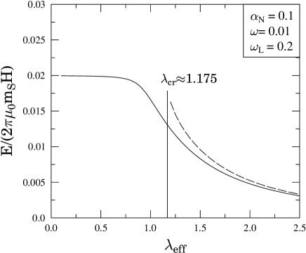
Figure 7: The energy loss is plottes versus the anisotropy $\lambda_{{\mathrm{eff}}}$. There are two scaling regimes, the one is at small, the other is at large anisotropy which are separated by the critical value $\lambda_{{\mathrm{cr}}}$. The full line corresponds to energy loss obtained at the stable fixed point below the equator and the dashed line represents energy loss at the fixed point above the equator which is stable only for $\lambda_{{\mathrm{eff}}}>\lambda_{{\mathrm{cr}}}$.

Thus, according to our results, the anisotropy (where the easy axis is perpendicular to the rotating external field) cannot be used to increase the heating efficiency of magnetic nanoparticles in the low-frequency limit.

For the sake of completeness let us consider the high-frequency limit, although it is out of the scope of the present work (irrelevant in case of cancer therapy by hyperthermia), hence, we do not study this in detail. The phase diagram obtained in the high-frequency and large anisotropy limit is shown in Fig. 8 and can be compared to the one obtained for low frequencies (with the same anisotropy), see Fig. 4.

Figure 8: Phase portrait in the rotating frame obtained by solving the LLG equation (III) in the limit of high-frequency and large anisotropy for the parameters $\alpha_{N}=0.1,\omega=0.15,\omega_{L}=0.2$ and $\lambda_{{\mathrm{eff}}}=2.5$. There are two attractive fixed points in the figure similarly to the low-frequency case, Fig. 4. Here the attractive fixed points have different y-components, thus the corresponding energy losses also differ from each other.

The similarity between the high and low frequency cases is that two attractive fixed points appear. However, in the high-frequency case they have different coordinates in the ($\phi$-$\theta$) plane. Thus, the energy losses correspond to the attractive fixed points differ from each other.

In summary we conclude that the uniaxial anisotropy (where the easy axis is perpendicular to the rotating external field) either does not modify the energy loss per cycle (in case of small anisotropy) or the energy dissipated is decreased as compared to the isotropic case.

IV Linearly polarized applied field in the limit of large anisotropy

One of the goal of this paper is to investigate the role of anisotropy in the possible enhancement of heat efficiency of magnetic nanoparticles driven by a rotating magnetic field. On the one hand, in the previous section it was obtained that in case of circularly polarized applied field if the uniaxial anisotropy (perpendicular to the rotating external field) has been taken into account, the energy loss per cycle either remains unchanged (small anisotropy) or decreased (large anisotropy). On the other hand, in Ref. Chatel2009 it was shown that for isotropic nanoparticles the linearly polarized external field provides us a larger heat power in the limit of low frequency. Furthermore, the latter statement was shown Raikher2011 to be reliable in the presence of thermal effect, too. Thus, the circularly polarized applied field cannot be used to achieve a better heating efficiency by nanoparticle systems (neither for isotropic, nor for anisotropic nanoparticles with uniaxial anisotropy) if the effect of thermal fluctuations is negligible. The role of thermal effects is discussed in V where it is argued that the possible modification of the above finding by thermal fluctuations can only be expected in case of moderate anisotropy. Thus, the results of the present work indicates that the heating efficiency cannot be increased by the rotating field at least for small and very large anisotropy in the limit of low frequencies (independently whether thermal effect are included or not). This finding does not require any further analysis of the linearly polarized applied field.

However, the study of energy losses in case of the linearly polarized applied field for anisotropic nanoparticles enables us to consider whether the large anisotropy can be used to explain the experimental results of Ahsen2010 . Let us note the formation of chains by nanoparticles is a known feature of ferrofluids and the chains of particles represents a very large anisotropy He . Therefore, in this section we discuss the solution of the LLG equations (1) obtained for a single-domain magnetic nanoparticle under linearly polarized, i.e. alternating applied (external) magnetic field in the limit of large anisotropy. The applied field is assumed to oscillate along the x-axis with an angular frequency $\omega$

$${\bf H_{{\mathrm{ext}}}} = \frac{\omega_{L}}{\gamma^{\prime}}\,\,(\cos(\omega t),0,0),$$ (23)

where $\omega_{L}=\gamma^{\prime}|{\bf H}|$ is the Larmor frequency. Similarly to the circularly polarized case, here, we consider particles with uniaxial anisotropy. The easy axis of the magnetization is chosen to be the x-axis (similar results can be obtained if it is chosen to be perpendicular to the x-axis)

$${\bf H_{{\mathrm{aniso}}}} = \frac{\omega_{L}}{\gamma^{\prime}}\,\,(\lambda_{{\mathrm{eff}}}M_{x},0,0),$$ (24)

where $M_{x}$ is the x-component of the magnetization vector and the parameter $\lambda_{{\mathrm{eff}}}$ describes the strength of the anisotropy. Note that in case of alternating applied field, it is convenient to study the original LLG equation (1) instead of the rotated one (III). The LLG equation for the Cartesian coordinates of the magnetization reads as

$$\frac{{\mathrm{d}}M_{x}}{{\mathrm{d}}t}=\alpha_{N}(\lambda_{{\mathrm{eff}}}M_{x}+\cos(\omega t))(1-M_{x}^{2}),$$

$$\frac{{\mathrm{d}}M_{y}}{{\mathrm{d}}t}=-(\omega_{L}M_{z}+\alpha_{N}M_{x}M_{y})(\cos(\omega t)+\lambda_{{\mathrm{eff}}}M_{x}),$$

$$\frac{{\mathrm{d}}M_{z}}{{\mathrm{d}}t}=(\omega_{L}M_{y}+\alpha_{N}M_{x}M_{z})(\cos(\omega t)+\lambda_{{\mathrm{eff}}}M_{x}),$$ (25)

which has in general no analytic solution. In the limit of extremely large anisotropy, $\cos(\omega t)\ll\lambda_{{\mathrm{eff}}}M_{x}$, however, the time-dependence of $M_{x}$ can be determined as

$$M_{x}(t)=\pm\frac{\exp(\alpha_{N}\lambda_{{\mathrm{eff}}}t)}{\sqrt{\exp(2\alpha_{N}\lambda_{{\mathrm{eff}}}t)-C}},$$ (26)

with $C=1-1/M_{x0}^{2}$. If $t\to\infty$ the solution (26) tends to $\pm 1$ and the energy loss per cycle vanishes.

We conclude that in case of a very large anisotropy the heat power of a magnetic nanoparticle driven by a linearly polarized applied field vanishes. The same was observed in case of the circularly polarized external field. Thus, it is a natural requirement to obtain a comparable heat power given by the linearly and the circularly polarized applied fields if the anisotropy is large enough which can explain the experimental results of Ahsen2010 . Indeed, if the ferrofluid was not prepared appropriately, the nanoparticles can form chains and consequently, the anisotropy could become large and the energy loss tends to zero rapidly.

V Thermal effects

In this work we studied the influence of anisotropy on the energy losses in the framework of the deterministic LLG equation in the absence of thermal fluctuations for rotating applied field. In this subsection, we discuss briefly how thermal effects (see e.g. stochastic_llg_lin ; stochastic_llg ; JaHaCh2012 ) can possibly modify the results obtained by considering purely dynamical effects based on the LLG equation. Let us follow Refs. Denisov2006 ; Denisov2006prl ; Denisov_thermal . In case of a rotating field, the steady state solutions of the dynamical problem are independent of the initial conditions of the individual particles. Therefore, the average magnetization can be easily determined by these (stable) steady states.

In case of two steady state magnetizations (up and down states), due to thermal effects, a nonzero probability of a transition from one stable state to another appears. This type of relaxation mechanism is missing in the present work due to the lack of thermal effects. We showed that large anisotropy is needed in order to have more then one stable state. It was also shown that if the anisotropy is not large enough only a single fixed point appear in the phase portrait, thus one has to consider only a single stable state. In this case the modification caused by thermal effects is less important. Thus, thermal effects can only modify the determination of energy losses (in case of a rotating applied field, for low frequencies relevant to hyperthermia) if the anisotropy is large enough but not too large (otherwise the barrier between one state to an other becomes too large).

Furthermore, let us compare Raikher2011 and Chatel2009 in order to consider the role of thermal effects in case of isotropic samples. In these articles energy losses were investigated both for alternating and for rotating applied field. Thermal effects were included in Raikher2011 while these are absent in Chatel2009 . For example, the dashed lines on Fig. 6 of Raikher2011 correspond to the limit $T\to 0$ and agree to the findings plotted in Fig. 2a of Chatel2009 qualitatively. Let us pay the attention of the reader to the logarithmic scale used in Fig. 2a of Chatel2009 . The modification caused by thermal effects (solid lines in Fig. 6) are less important for the rotating case but very significant for the alternating case in the limit of low frequencies. Nevertheless, for low frequencies, the linearly polarized field was found to produce more heat power both for $T=0$ and for $T\neq 0$.

According to Refs. Denisov2006 ; Denisov2006prl ; Denisov_thermal for small and for very large anisotropy the thermal effects are less important. It was shown in Ref. Raikher2011 that for isotropic samples even for $T\neq 0$ the energy absorption per cycle for a nanoparticle was larger in case of a linearly polarized applied field. Thus, if anisotropy (at least if it is small or very large) does not increase the energy losses obtained in case of a rotating external field (which is one of the finding of the present work), a better heating efficiency can be achieved for isotropic nanoparticles using linearly polarized field. This indicates that possible modification caused by thermal effects can only be expected in case of moderate anisotropy. Therefore, the study of the present work is relevant for applications in hyperthermia at least for small and very large anisotropy.

VI Summary

The nonlinear dynamics of magnetization and the loss energy of a single magnetic nanoparticle with uniaxial anisotropy have been considered under circularly polarized applied field in the absence of thermal fluctuations. The easy axis of magnetization has been chosen to be perpendicular to the rotating applied field. We solved the deterministic Landau-Lifshitz-Gilbert equation in order to determine the loss energy per cycle in case of the rotating applied field and the findings were compared to that of obtained for the isotropic case in Chatel2009 . Comparison between the linearly and circularly polarized applied field has also been performed and the results were analyzed in terms of the experimental data Ahsen2010 .

Our goal was twofold: (i) to study whether the anisotropy can be used to achieve a better heating efficiency in case of rotating external field, (ii) to use the anisotropy to resolve the discrepancy between theory Chatel2009 and experiment Ahsen2010 . We showed that for circularly polarized field, the loss energy per cycle is decreased by the anisotropy compared to the isotropic case. Thus in the low-frequency limit, more heat power can be achieved by alternating applied field for isotropic nanoparticles, at least the rotating applied field produces lower energy absorption for small and very large anisotropy. It was also shown that in the limit of extremely large anisotropy, experimental results of Ahsen2010 can be explained. The possible role of thermal fluctuations discussed here indicates the necessity of the extension of the present study for the case of moderate anisotropy when thermal effects are taken into account appropriately.

References

- (1) C. Scherer, H.G. Matuttis, Phys. Rev. E 63 011504 (2000); J. Embs, H. W. Müller, C. Wagner, K. Knorr, and M. Lücke, Phys. Rev. E 61, R2196 (2000); B. U. Felderhof, Phys. Rev. E 62, 3848 (2000); M.I. Shliomis, Phys. Rev. E 64, 063501 (2001); B. U. Felderhof, Phys. Rev. E 64, 063502 (2001); H.W. Müller and M. Liu, Phys. Rev. E 64, 061405 (2001); J. P. Embs, S. May, C. Wagner, A. V. Kityk, A. Leschhorn, and M. Lücke, Phys. Rev. E 73, 036302 (2006); A. Leschhorn, M. Lücke, C. Hoffmann and S. Altmeyer, Phys. Rev. E 79, 036308 (2009).
- (2) M.I. Shliomis, Zh. Eksp. Teor. Fiz. 61, 2411 (1971) [Sov. Phys. JETP 34, 1291 (1972)]; M.I. Shliomis, Usp. Fiz. Nauk 112, 427 (1974) [Sov. Phys. Usp. 17, 153 (1974)];. R.E. Rosensweig, Ferrohydrodynamics, Cambridge University Press, Cambridge, (1985); M.I. Shliomis, Phys. Rev. E 64, 060501(2001);
- (3) M. V. Petrova, et al., Applied Magnetic Resonance 41, 525 (2011).
- (4) Q. A. Pankhurst, J. Connolly, S. K. Jones, and J. Dobson, J. Phys. D: Appl. Phys. 36, R167 (2003); M. Ferrari, Nat. Rev. Cancer 5, 161 (2005); R. Hergt, S. Dutz, R. Muller, M. Zeisberger, J. Phys.: Condens. Matter 18 S2919 (2006); R. Hergt, S. Dutz, J. Magn. Magn. Mater. 311, 187 (2007); S. Laurent, D. Forge, M. Port, A. Roch, C. Robic, L. Vander Elst, and R. N. Muller, Chem. Rev. 108, 2064 (2008); J. D. Alper, Thesis (Ph.D.), Massachusetts Institute of Technology (2010); Quian Wang and Jing Liu, Fundamental Biomedical Technologies 5, 567-598 (2011), Spinger Science+Business Media: Intercellular Delivery (ed. A. Prokop); A. L. E. Rast, Thesis (Ph.D.) University of Alabama, Birmingham (2011); D. E. Bordelon, C. Cornejo, C. Grüttner, F. Westphal, T. L. DeWeese, R. Ivkov, J. Appl. Phys. 109, 124904 (2011); A. Arakaki, K. Shibata, T. Mogi, M. Hosokawa, K. Hatakeyama, H. Gomyo, T. Taguchi, H. Wake, T. Tanaami, T. Matsunaga and T. Tanaka, Polymer Journal 44, 672 (2012).
- (5) Yu. L. Raikher and V. I. Stepanov, Phys. Rev. E 83, 021401 (2011).
- (6) P. Cantillon-Murphy, L.L. Wald, E. Adalsteinsson, M. Zahn, JMMM 322, 727 (2010).
- (7) O. O. Ahsen, U. Yilmaz, M. D. Aksoy, G. Ertas, E. Atalar, JMMM 322, 3053 (2010).
- (8) W. T. Coffey and P. C. Fannin, J. Phys.: Condens. Matter 14, 3677 (2002); P. Moroz, S. K. Jones and B. N. Gray, Int. J. Hyperthermia 18, 267 (2002).
- (9) I. S. Poperechny, Yu. L. Raikher, and V. I. Stepanov, Phys. Rev. B 82, 174423 (2010).
- (10) P. F. de Châtel, I. Nándori, J. Hakl, S. Mészáros and K. Vad, J. Phys.: Condens. Matter 21, 124202 (2009).
- (11) Giorgio Bertotti, Claudio Serpico, and Isaak D. Mayergoyz, Phys. Rev. Lett. 86, 724 (2001).
- (12) S. I. Denisov, T. V. Lyutyy, P. Hänggi, K. N. Trohidou, Phys. Rev. B 74, 104406 (2006).
- (13) Z. Z. Sun, X. R. Wang, Phys. Rev. B 73, 092416 (2006).
- (14) S. I. Denisov, T. V. Lyutyy, P. Hänggi, Phys. Rev. Lett. 97, 227202 (2006).
- (15) S. I. Denisov, T. V. Lyutyy, C. Binns, P. Hänggi, JMMM 322, 1360 (2010); S. I. Denisov, A. Yu. Polyakov, and T. V. Lyutyy, Phys. Rev. B 84, 174410 (2011).
- (16) L. Néel, Compt. rend. Acad. Sci. (Paris) 228, 664 (1949).
- (17) L. Landau and E. Lifshitz, Phys. Z. Sowjetunion 8, 153 (1935).
- (18) T. L. Gilbert, Phys. Rev. 100, 1243 (1955).
- (19) W. F. Brown, Jr., Phys. Rev. 130, 1677 (1963); ibid IEEE Trans. Magn. 15, 1196 (1979).
- (20) T. L. Gilbert, IEEE Trans. Magn. 40, 3443 (2004).
- (21) L-M. He, Commun. Theor. Phys. 55 (2011) 537.
- (22) H. El Mrabti, S. V. Titov, P.M. Déjardin, Y. P. Kalmykov, J. Appl. Phys. 110, 023901 (2011); H. El Mrabti, P.M. Déjardin, S. V. Titov, Y. P. Kalmykov, Phys. Rev. B 85, 094425 (2012).
- (23) Denis M. Basko, Maxim G. Vavilov, Phys. Rev. B 79, 064418 (2009); Thomas Bose, Steffen Trimper, Phys. Rev. B 81, 104413 (2011).
- (24) Zs. Jánosfalvi, J. Hakl, P. F. de Châtel, arXiv:1201.5236 [cond-mat.mes-hall].