Nuclear Level Densities in the Constant–Spacing Model

Abstract

A new method to calculate level densities for non–interacting Fermions within the constant–spacing model with a finite number of states is developed. We show that asymptotically (for large numbers of particles or holes) the densities have Gaussian form. We improve on the Gaussian distribution by using analytical expressions for moments higher than the second. Comparison with numerical results shows that the resulting sixth–moment approximation is excellent except near the boundaries of the spectra and works globally for all particle/hole numbers and all excitation energies.

I Purpose

Our interest in the dependence of various nuclear level densities on energy and particle number has been triggered by recent experimental developments in laser physics. The Extreme Light Infrastructure (ELI) eli will open new possibilities for extremely high–intensity laser interactions with fundamental quantum systems different from the traditionally considered atoms and molecules Di12 . At the Nuclear Physics Pillar of ELI under construction in Romania, efforts are under way to generate a multi–MeV zeptosecond pulsed laser beam Mor11 . For medium–weight and heavy target nuclei interacting with such a beam, photon coherence can cause multiple photon absorption. With energies of several MeV per photon, the ensuing nuclear excitation energies may well amount to several $100$ MeV. Depending on the time scale on which the excitation takes place and on the specific nucleon-nucleon interaction rates, collective excitations may be induced, or a compound nucleus be formed Wei11 . A theoretical treatment of the latter process along the lines of precompound reaction models requires the knowledge of the total level density, of the densities of $p$–particle $h$–hole states, and of the density of accessible states for particle/hole numbers and/or excitation energies that go far beyond what has been considered until now. That applies not only to the target nucleus but also to all daughter nuclei populated by induced particle emission during the interaction time of the laser pulse.

The standard approach to level densities goes back to the pioneering work of Bethe Bet36 who calculated the total level density as a function of excitation energy with the help of the Darwin–Fowler method. Basically the same method was used in many of the later works Eri60 ; Boe70 ; Wil71 ; Sta85 ; Obl86 ; Her92 dealing with the density of $p$–particle $h$–hole states and related quantities. A beautiful review is given in Ref. Blo68 . The Darwin–Fowler method yields analytical expressions involving contour integrals. Their evaluation, although straightforward, becomes increasingly involved with increasing numbers of particles and holes and/or increasing excitation energy. The same is true for Refs. Gho83 ; Bli86 that account for the exclusion principle by explicit counting. Moreover, without explicit numerical calculation it is not possible within these approaches to establish general properties of particle–hole densities like the overall dependence on excitation energy and/or particle–hole number. More recent works use a static–path approximation (Refs. Lau89 ; Alh93 and papers cited therein) or account, in addition, for the residual interaction in an approximate way (Ref. Can94 and references therein). The method of Ref. Hil98 avoids contour integrals and determines (again numerically) the level densities directly as coefficients of polynomials. The order of these rises rapidly, too, with energy and particle/hole number. In none of these approaches does it seem possible to deal with the enormously large values of the various densities attained for medium–weight and heavy nuclei at excitation energies of several $100$ MeV in a practicable way. That is why we develop a different approach in the present work.

In this Letter we present an analytical approximation to the global dependence of partial and total level densities that takes full account of the exclusion principle, that is valid for a finite number of single–particle states, and that holds for all excitation energies and particle/hole numbers. We prove analytically that the level density for particles or holes is for a constant–spacing model asymptotically Gaussian. We improve on the Gaussian using analytical results for the low moments of the distribution higher than the second. Comparison with numerical results shows that the resulting sixth–moment approximation is very precise except near the boundaries of the spectrum (where numerical evaluation is easy). Particle–hole densities follow by convolution. The attained analytical form of the global dependence of level densities on excitation energy and particle number extends our understanding of characteristic nuclear properties into uncharted territory. Moreover, we expect our results to be an indispensable tool in the calculation of laser–induced nuclear reactions mentioned in the first paragraph.

We calculate the various densities in the framework of a constant–spacing model for spinless non–interacting Fermions. To justify our choice we consider by way of example the partial level density $\rho_{p}(E,J,\pi)$ for $p$ particles and $p$ holes, a function of excitation energy $E$, total spin $J$, and parity $\pi$, for a system of non–interacting Fermions in three dimensions. For other densities the reasoning is the same. The partial level density is given by Her92

$$\rho_{p}(E,J,\pi) = (1/2)\rho_{p}(E)\ \frac{2J+1}{2\sqrt{2\pi}\ \sigma^{3}_{2p}}$$ (1)

$$\times \exp\bigg{\{}-\frac{[J+(1/2)]^{2}}{2\sigma^{2}_{2p}}\bigg{\}}\ .$$

The factor $1/2$ accounts for parity. The last two terms of the product give the spin dependence, with $\sigma_{2p}$ the spin–cutoff factor. With spin and parity being accounted for, $\rho_{p}(E)$ is defined as the level density of spinless non–interacting Fermions that carry no angular momentum. We note that in preequilibrium theories, the interactions between Fermions neglected here are taken into account as agents for equilibration. In our model, the non–interacting Fermions are distributed over a set of single–particle states. Each subshell with spin $j$ of the three-dimensional shell model contributes $(2j+1)$ states to the set. For large excitation energy or particle–hole numbers, we must take into account the exclusion principle exactly. It is equally important to account for the finite binding energy of particles and for the finite size of the energy interval available for holes. Both strongly affect the various level densities at large excitation energies. We do so using a single–particle model with a finite number of states. Moreover, we calculate the various densities using a constant–spacing model for the single–particle states. It is clear from the shell model that the model is not realistic at the high excitation energies of interest. Taking into account the multiplicity $(2j+1)$ of the subshells, we note that the single–particle level density of the shell model strongly increases with energy. We return to this point at the end of Section V.

II Approach

We consider $f$ spinless Fermions in a single–particle model with constant level spacing $d$ and with a finite number $u$ of bound single–particle states. In the ground state all single–particle states from the lowest (energy $d$) up to a maximum level (energy $F=fd$ with $F$ for Fermi energy) are occupied. The remaining $b=B/d$ levels (with $B$ for binding energy) are empty. Here $f$ and $b$ are integers, and we have $u=f+b$. Excited states are described as $p$–particle $h$–hole states, with $p$ counting the number of particles in single–particle states with energy larger than $F$ and not larger than $B+F$, and correspondingly $h$ counting the number of holes with energy less than $F$. For non–closed shell compound nuclei and/or nuclear reactions induced by composite particles, the number of hole states $h$ may differ from $p$. We calculate various many–body level densities for non–interacting particles: $\rho_{B}(p,E)$ is the level density versus energy $E$ for $p$ particles confined to an energy interval of length $B$, $\rho_{F}(h,E)$ is the level density for $h$ holes confined to an energy interval of length $F$, $\rho_{FB}(p,h,E)$ is the particle–hole state density defined analogously, and $\rho_{U}(A,E)$ is the total level density for $A$ particles distributed over an energy interval of length $U=F+B$. With $\varepsilon=E/d$ and $\varepsilon$ integer we define the dimensionless density $\omega_{b}(p,\varepsilon)=\rho_{B}(p,E)\,d$ and analogously for $\omega_{f}(h,\varepsilon)$, $\omega_{fb}(p,h,\varepsilon)$, and $\omega_{u}(A,\varepsilon)$. All densities denoted by $\omega$ are integers.

We describe the method of calculation for $\omega_{b}(p,\varepsilon)$, assuming for simplicity of notation that $b$ is odd and shifting the energy such that the ground state of the $p$–particle system has energy $(1/2)p(p+1)$. The maximum energy is $bp-(1/2)p(p-1)$, and the center of the spectrum is at

$$\varepsilon^{(0)}_{b}(p)=\frac{1}{2}p(b+1)\ .$$ (2)

The level density $\omega_{b}(p,\varepsilon)$ is defined as the number of ways in which $p$ Fermions can be distributed over the $b$ available single–particle states such that the total energy equals $\varepsilon$, i.e.,

$$\omega_{b}(p,\varepsilon)=\sum_{1\leq n_{1}<n_{2}<\ldots<n_{p}\leq b}\delta_{n_{1}+n_{2}+\ldots+n_{p},\,\varepsilon}\ .$$ (3)

The calculation of $\omega_{b}(p,\varepsilon)$ poses a purely combinatorial problem. With $\beta=(1/2)(b-1)$ we define new summation variables $k_{l}=n_{l}-(1/2)(b+1)$, $l=1,2,\ldots,p$ that range from $-\beta$ to $+\beta$. With $\varepsilon^{\prime}=\varepsilon-\varepsilon_{0}(p)$ that gives

$$\omega_{b}(p,\varepsilon^{\prime})=\sum_{-\beta\leq k_{1}<k_{2}<\ldots<k_{p}\leq\beta}\delta_{k_{1}+k_{2}+\ldots+k_{p},\,\varepsilon^{\prime}}\ .$$ (4)

We determine $\omega_{b}(p,\varepsilon^{\prime})$ in terms of its low moments. Changing the signs of all summation variables in Eq. (4) one can easily show that $\omega_{b}(p,\varepsilon^{\prime})=\omega_{b}(p,-\varepsilon^{\prime})$ is even in $\varepsilon^{\prime}$, so that all odd moments vanish. For the $2m$th moment with $m=0,1,2,\ldots$ we have

$$m_{b}(p,2m) = \sum_{\varepsilon^{\prime}}(\varepsilon^{\prime})^{2m}\omega_{b}(p,\varepsilon^{\prime})$$ (5)

$$= \sum_{-\beta\leq k_{1}<k_{2}<\ldots<k_{p}\leq\beta}\ \bigg{(}\sum_{l}k_{l}\bigg{)}^{2m}\ .$$

Following Ref. Boe70 we adopt an occupation–number representation for Fermionic many–body states. We represent each set $\{k_{l}\}$ of integers in Eq. (4) as a $b$–dimensional vector $\{\nu_{1},\nu_{2},\ldots,\nu_{b}\}$ with entries $\nu_{j}$ that take values zero and one. The set $\{k_{l}\}$ is represented by choosing $\nu_{j}=1$ in the $p$ positions $k_{l}$ and zero otherwise. The sum over all $\{k_{l}\}$ is replaced by the sum over all $b$–dimensional vectors, i.e., over all choices of $\nu_{j}$ subject to the constraint $\sum_{j}\nu_{j}=p$. Thus,

$$m_{b}(p,2m)=\sum_{\nu_{1},\nu_{2},\ldots,\nu_{b}}\delta_{p,\nu_{1}+\nu_{2}+\ldots+\nu_{b}}\ \bigg{(}\sum_{j}j\nu_{j}\bigg{)}^{2m}$$

$$=\frac{\partial^{2m}}{\partial\sigma^{2m}}\sum_{\nu_{1},\nu_{2},\ldots,\nu_{b}}\delta_{p,\nu_{1}+\nu_{2}+\ldots+\nu_{b}}\exp\{\sigma\sum_{j}j\nu_{j}\}\bigg{|}_{\sigma=0}\ .$$ (6)

We multiply Eq. (6) with $\exp\{p\alpha\}$, sum over $p$, and carry out the summations over the $\nu_{j}$. This gives the partition function

$$Z_{b}(\alpha,2m)=\frac{\partial^{2m}}{\partial\sigma^{2m}}\prod_{j=-\beta}^{\beta}(1+\exp\{\alpha+\sigma j\})\bigg{|}_{\sigma=0}\ .$$ (7)

The moment $m_{b}(p,2m)$ is the coefficient multiplying $\exp\{\alpha p\}$ in an expansion of $Z_{b}(\alpha,2m)$ in powers of $\exp\{\alpha\}$. For $m=0$ we find $m_{b}(p,0)$ $={b\choose p}$, the correct result. For $m=1,2$ we obtain

$$m_{b}(p,2) = \bigg{(}\sum_{j=-\beta}^{\beta}j^{2}\bigg{)}{b-2\choose p-1}\ ,$$

$$m_{b}(p,4) = \bigg{(}\sum_{j=-\beta}^{\beta}j^{4}\bigg{)}\bigg{[}{b-4\choose p-1}-4{b-4\choose p-2}+{b-4\choose p-3}\bigg{]}$$ (8)

$$+3\bigg{(}\sum_{j=-\beta}^{\beta}j^{2}\bigg{)}^{2}{b-4\choose p-2}\ .$$

From Eqs. (8) we obtain the normalized moments

$$M_{b}(p,2m)=\frac{m_{b}(p,2m)}{m_{b}(p,0)}\ .$$ (9)

III Asymptotically Gaussian Distribution

Eqs. (8) suggest that asymptotically ($b\gg 1$, $p\gg 1$) $\omega_{b}(p,\varepsilon^{\prime})$ approaches a Gaussian distribution. (Here, with $1\leq p\leq b$ and $b\gg 1$, we consider $p\gg 1$ equivalent to $p\approx b/2$. Particle–hole symmetry connects the cases $p\approx b$ and $p\approx 1$). We recall that for a Gaussian distribution, the normalized fourth moment (see Eq. (9)) equals three times the square of the normalized second moment. For $b\gg 1$ and $p\gg 1$ that is exactly the relation implied by the values of $m_{b}(p,4)$ and $m_{b}(p,2)$ in Eq. (8). Indeed, taken by itself the last term in the expression for $m_{b}(p,4)$ yields a value for $M_{b}(p,4)$ which for $b\gg 1$, $p\gg 1$ equals three times the square of $M_{b}(p,2)$. Moreover, the term proportional to $\sum j^{4}$ in the expression for $m_{b}(p,4)$ is smaller by the factor $1/p$ than the one proportional to $(\sum j^{2})^{2}$. To show that $\omega_{b}(p,\varepsilon^{\prime})$ becomes asymptotically ($b\gg 1,p\gg 1$) Gaussian we generalize the approach of Eqs. (6) to (8) to all moments. We define

$$G(\sigma)=\prod_{j=-\beta}^{\beta}(1+\exp\{\alpha+\sigma j\})=\exp\{H(\sigma)\}$$ (10)

and expand $H(\sigma)$ in a Taylor series around $\sigma=0$. With

$$f(\alpha)=\frac{\exp\{\alpha\}}{1+\exp\{\alpha\}}$$ (11)

and $f^{(n)}$ denoting the $n$th derivative of $f$, we have for $m=1,2,\ldots$

$$\frac{\partial^{m}}{\partial\sigma^{m}}H(\sigma)\bigg{|}_{\sigma=0}=f^{(m-1)}\sum_{j=-\beta}^{\beta}j^{m}\ .$$ (12)

This shows that all odd derivatives of $H$ vanish. We insert the Taylor expansion for $H$ into Eq. (10) and obtain

$$G(\sigma)=G(0)\exp\bigg{\{}\sum_{n=1}^{\infty}\frac{1}{(2n)!}\sigma^{2n}f^{(2n-1)}\sum_{j=-\beta}^{\beta}j^{2n}\bigg{\}}\ .$$ (13)

From here, we proceed in two steps. (i) We neglect all terms with $n>1$ on the right–hand side of Eq. (13) and show that as a result, $\omega_{b}$ is Gaussian for $b\gg 1$, $p\gg 1$. (ii) We show by complete induction that all terms with $n>1$ in Eq. (13) are negligibly small in the same limit. (i) For $\omega_{b}(p,\varepsilon^{\prime})$ to be Gaussian we have to show that $M_{b}(p,2m)=(2m-1)!!\ [M_{b}(p,2)]^{m}$. Taking into account the term with $n=1$ only, expanding the exponential, and using the result in Eqs. (10) and (7) we obtain

$$Z_{b}(\alpha,2m)=(2m-1)!!\ G(0)(f^{\prime})^{m}\bigg{(}\sum_{j=-\beta}^{\beta}j^{2}\bigg{)}^{m}\ .$$ (14)

The normalized $2m$th moment $M_{b}(p,2m)$ is the coefficient multiplying $\exp\{p\alpha\}$ in the expansion of $Z_{b}(\alpha,2m)$ in powers of $\exp\{\alpha\}$ divided by the normalization factor ${b\choose p}$. For $b\gg 1$ and $p\gg 1$ the relevant coefficient in $G(0)(f^{\prime})^{m}{b\choose p}^{-1}$ is $\approx[p(b-p)b^{-2}]^{m}$. That yields $M_{b}(p,2m)\approx(2m-1)!!\ [M_{b}(p,2)]^{m}$, consistent with a Gaussian form for $\omega_{b}(p,\varepsilon^{\prime})$. In the last step of the argument we approximate products of the form $p(p-1)\ldots(p-m)$ by $p^{m}$. For fixed $p$ the approximation becomes increasingly inaccurate as $m$ increases. Our result is therefore valid only asymptotically. (ii) We use complete induction to show that the contributions of the terms with $n>1$ in Eq. (13) become vanishingly small for $b\gg 1,p\gg 1$. We have shown above that this claim holds for $n=2$ (i.e., for $m_{b}(p,4)$). We assume that the claim is correct for $2\leq n<n_{0}$, omit the corresponding terms in Eq. (13), and show that it holds for $n=n_{0}$, i.e., for $M_{b}(p,2n_{0})$. We have shown under (i) that the contribution to $M_{b}(p,2n_{0})$ of the term with $n=1$ is $(2n_{0}-1)!!\ (M_{b}(p,2))^{n_{0}}$. The contribution of the term with $n=n_{0}$ is $G(0)f^{(2n_{0}-1)}\sum_{j}j^{2n_{0}}$. For $b\gg 1$ we have $\sum_{j}j^{m}\approx b^{m+1}/(2^{m}(m+1))$. From Eq. (11) we have $f^{\prime}=f-f^{2}$. Therefore, $f^{(2n_{0}-1)}=\sum_{l=1}^{2n_{0}}c_{l}f^{l}$ is a polynomial of degree $2n_{0}$ in $f$ with integer coefficients $c_{l}$, and the contribution of $G(0)f^{(2n_{0}-1)}\sum_{j}j^{2n_{0}}$ to $M_{b}(p,2n_{0})$ is

$${b\choose p}^{-1}\frac{b^{2n_{0}+1}}{(2n_{0}+1)2^{2n_{0}}}\sum_{l=1}^{2n_{0}}c_{l}{b-2n_{0}\choose p-l}\ .$$ (15)

For $b\gg 2n_{0}$ and $p\gg l$ we have ${b-2n_{0}\choose p-l}\approx{b\choose p}p^{l}/b^{l}$. The contribution (15) is, therefore, of order $b^{2n_{0}+1}$ while the contribution from the term with $n=1$ is of order $b^{3n_{0}}$. This shows that the contributions with $n=1$ dominate all others. The situation differs for $b\gg 1$ and $p\approx 1$ or $p\approx b$ where $M_{b}(p,2)$ is of order $b^{2}$ only and $[M_{b}(p,2)]^{n_{0}}$ is comparable in size to the contribution (15). Here the Gaussian approximation cannot be expected to work well. This is consistent with the fact that for $p=1$ and $p=b-1$ the densities are flat, $\omega_{b}(1,\varepsilon^{\prime})=1=\omega_{b}(b-1,\varepsilon^{\prime})$. Furthermore, for $p=2$ and $p=b-2$ the densities have a triangularly shaped maximum. Only with $p=3$ and $p=b-3$ does the density of states become Gaussian–shaped. The maximum at $\varepsilon^{\prime}=\varepsilon^{(0)}_{b}(p)$ builds up only slowly as $p$ increases from unity or decreases from $b-1$.

IV Low-Moments Approximation

Using the asymptotically Gaussian form of $\omega_{b}(p,\varepsilon^{\prime})$ we approximate that function in terms of its low even moments. We use Eqs. (8) for $m_{b}(p,2)$ and $m_{b}(p,4)$, calculate $m_{b}(p,6)$ similarly, and find the parameters $\gamma_{2m}$, $m=1,2,3$ of the normalized function

$$F^{(6)}_{b}(p,\varepsilon^{\prime})=C\exp\{-\gamma_{2}(\varepsilon^{\prime})^{2}-\gamma_{4}(\varepsilon^{\prime})^{4}-\gamma_{6}(\varepsilon^{\prime})^{6}\}$$ (16)

that correspond to the normalized moments $M_{b}(p,2m)$ with $m=1,2,3$ in Eq. (9). The resulting function

$$\omega^{(6)}_{b}(p,\varepsilon^{\prime})={b\choose p}F^{(6)}_{b}(p,\varepsilon^{\prime})$$ (17)

is referred to in the following as the sixth–moment approximation to $\omega_{b}(p,\varepsilon^{\prime})$. Approximations obtained by using only the second (only the second and the fourth) moment(s) are denoted by $\omega^{(2)}_{b}(p,\varepsilon^{\prime})$ (by $\omega^{(4)}_{b}(p,\varepsilon^{\prime})$, respectively). The same approach is used for $\omega_{f}(h,\varepsilon^{\prime})$ and for $\omega_{u}(A,\varepsilon)$. Except for suitable changes of indices and parameters, the results are formally identical. We mention in passing that the method is also useful for calculating the density of accessible states Obl86 ; Car12 under the constraints of the exclusion principle. Details will be given elsewhere. For the $p$–particle $h$–hole density $\omega_{bf}(p,h,\varepsilon)$ we define $\varepsilon$ as the total excitation energy of the Fermionic system. Then

$$\omega_{bf}(p,h,\varepsilon)=\sum_{\varepsilon_{p}\varepsilon_{h}}\delta_{\varepsilon_{p}+\varepsilon_{h},\,\varepsilon}\omega_{b}(p,\varepsilon_{p})\omega_{f}(h,\varepsilon_{h})\ .$$ (18)

Here $\varepsilon_{p}=\varepsilon^{(0)}(p)+\varepsilon^{\prime}_{p}$ is the total energy of the $p$ particles, and correspondingly for holes, while $\varepsilon=\varepsilon_{p}+\varepsilon_{h}$ is the excitation energy of the $p$–particle $h$–hole system. Thus

$$\omega_{bf}(p,h,\varepsilon)=\sum_{\varepsilon_{p}\varepsilon_{h}}\delta_{\varepsilon^{\prime}_{p}+\varepsilon^{\prime}_{h},\,\varepsilon-\varepsilon^{(0)}_{p}-\varepsilon^{(0)}_{h}}\omega_{b}(p,\varepsilon^{\prime}_{p})\omega_{f}(h,\varepsilon^{\prime}_{h})\ .$$ (19)

Since $\omega_{b}(p,\varepsilon^{\prime}_{p})$ ($\omega_{f}(h,\varepsilon^{\prime}_{h})$) is a symmetric function of $\varepsilon^{\prime}_{p}$ (of $\varepsilon^{\prime}_{h}$, respectively), it follows that $\omega_{bf}$ is a symmetric function of $\varepsilon$ centered at $\varepsilon^{(0)}=\varepsilon^{(0)}_{p}+\varepsilon^{(0)}_{h}$. Therefore we consider the function $\omega_{bf}(p,h,\varepsilon^{\prime})$ with $\varepsilon^{\prime}=\varepsilon-\varepsilon^{(0)}$. This function is symmetric about $\varepsilon^{\prime}=0$. For the low even moments we obtain

$$m_{bf}(p,h,0) = {b\choose p}\ {f\choose h}\ ,$$

$$m_{bf}(p,h,2) = m_{b}(p,2)+m_{f}(h,2)\ ,$$

$$m_{bf}(p,h,4) = m_{b}(p,4)+2m_{b}(p,2)m_{f}(h,2)$$ (20)

$$+m_{f}(h,4)\ ,$$

and correspondingly for higher moments.

V Numerical Results

We begin with an overview of the dependence of $\omega_{b}(p,\varepsilon)$ on both $p$ and $\varepsilon$ using the sixth–moment approximation (17). Even though we expect that approximation to work well only for $p\approx b/2$, we display in Fig. 1 the values of $\omega^{(6)}_{b}(p,\varepsilon)$ for $b=51$ in the $p$–$\varepsilon$ plane as a coloured contour plot for all values of $p$ between 3 and $b-3$. For fixed $p$, the dimensionless energy $\varepsilon$ takes values in the interval $(1/2)p(p+1)\leq\varepsilon\leq bp-(1/2)p(p-1)$. This accounts for the two nearly parabolic and sawtooth–like boundaries of the coloured domain. The parabolic dependence on $p$ is given by $(1/2)p(p+1)$ for the lower edge and by $bp-(1/2)p^{2}+(1/2)p$ for the upper edge. The contour plot is symmetric with respect to a simultaneous mirror reflection about the vertical line $p=(b-1)/2$ and about the horizontal line defined by the overall centroid energy $\varepsilon=(1/4)(b^{2}-1)$. This symmetry is due to the symmetry of $\omega_{b}(p,\varepsilon)$ in $\varepsilon$ about the centroid energy $\varepsilon^{(0)}_{b}(p)$, and to particle–hole symmetry which equates $\omega_{b}(p,\varepsilon)$ with $\omega_{b}(b-p,\varepsilon)$ except for a shift by the difference $\varepsilon^{(0)}_{b}(b-p)-\varepsilon^{(0)}_{b}(p)$ of the centroid energies. For fixed $p$, $\omega_{b}(p,\varepsilon)$ displays a maximum at $\varepsilon^{(0)}_{b}(p)=(1/2)p(b+1)$ (except for the cases $p=1$ and $p=b-1$ not displayed in the Figure). The location of the maximum increases linearly with $p$. This fact and the parabolic form of the boundaries cause the quasi–elliptical shape of the solid line of constant $\omega_{b}$–values in the colour plot. We note the enormous maximum values of $\omega_{b}(p,\varepsilon^{(0)}_{b}(p))\approx 10^{12}$ attained for $p\approx 25$. All these features are generic (i.e., independent of the performance of the sixth–moment approximation) and apply likewise to $\omega_{f}(h,\varepsilon^{\prime})$ and to $\omega_{u}(A,\varepsilon^{\prime})$, except for a rescaling of abscissa, ordinate, and of the values of the densities.

Limitations of the sixth–moment approximation become obvious when we consider the values of $\omega_{b}(p,\varepsilon)$ at the boundaries $\varepsilon=(1/2)p(p+1)$ and $\varepsilon=bp-(1/2)p(p-1)$ where we obviously must have $\omega_{b}(p,\varepsilon)\approx 1$. The sixth–moment approximation exceeds this value by one to two orders of magnitude, see Fig. 3 below. (We should keep in mind, of course, that the values at the boundaries predicted by the sixth–moment approximation are smaller by about $10$ orders of magnitude than the values in the maximum. The relative accuracy of the sixth–moment approximation is, therefore, excellent). The white dashed lines in Fig. 1 show at which values of $p$ and $\varepsilon$ the sixth–moment approximation deviates by $10\%$ from the exact values. The inaccuracy affects only the very tails of the density of states, symmetrically about the centroid energy $\varepsilon^{(0)}_{b}(p)$. The dashed lines thus follow the boundaries of $\omega_{b}(p,\varepsilon)$.

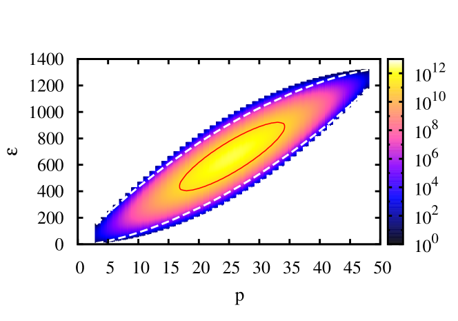
Figure 1: Contour plot of the dimensionless level density $\omega^{(6)}_{b}(p,\varepsilon)$ for $p$ particles in $b=51$ equally spaced single–particle states based on the sixth–moment approximation (17) versus $p$ and versus dimensionless energy $\varepsilon$. The white dashed lines define the boundary of the region where $\omega^{(6)}_{b}(p,\varepsilon)$ deviates by $10\%$ or more from the exact values. The full line presents the constant contour $\omega^{(6)}_{b}(p,\varepsilon)=10^{11}$.

We test the performance of the sixth–moment approximation in detail by a comparison with exact numerical results. This can be done throughout the critical domain (where either $p\approx 1$ or $p\approx b$ or where $\varepsilon$ is close to the boundary of the spectrum) since this is easily accessible numerically. We calculate the exact values of $\omega_{b}(p,\varepsilon)$ in two ways. (i) We directly use Eq. (4). (ii) We use the occupation–number representation defined above Eq. (6) and sum over all $b$–dimensional vectors $\{\nu_{1},\nu_{2},\ldots,\nu_{b}\}$, grouping the results according to particle number $p=\sum_{j}\nu_{j}$ and energy $\varepsilon^{\prime}=\sum_{j}j\nu_{j}$. Method (i) yields $\omega_{b}(p,\varepsilon)$ for fixed $b$ and $p$. Method (ii) yields $\omega_{b}(p,\varepsilon^{\prime})$ for fixed $b$ and all values of $p$ and $\varepsilon^{\prime}$. The demand on computing time is obviously larger for method (ii). Particle–hole densities are then obtained from Eq. (18). Our results agree with those of Ref. Obl86 for the small numbers of particles and holes considered there.

For the comparison between our exact and approximate results, we restrict ourselves to a few central features. In Fig. 2 we display the relative difference between the exact result and the sixth–moment approximation for $b=51$ and various values of $p$ near $b/2$. Significant deviations occur only at the boundaries of the spectrum where the values of the sixth–moment approximation are too large. Even though the tails of the sixth–moment approximation are suppressed by many orders of magnitude in comparison with the value at the center, that suppression is not strong enough. This is shown more clearly in Fig. 3 where we plot for $b=51$ the values of $\omega^{(2)}_{b}(p,\varepsilon)$, of $\omega^{(4)}_{b}(p,\varepsilon)$, and of $\omega^{(6)}_{b}(p,\varepsilon)$ (these functions are defined in and below Eq. (17)) versus $p$ at the boundary of the spectrum for $b=51$. With every additional moment included in the approximation, the agreement with the correct value $\omega_{b}\approx 1$ is drastically improved. However, it would obviously take even higher moments than the sixth one to reach quantitative agreement at the boundary of the spectrum. This can be done, although convergence may be slow. Alternatively, we may calculate $\omega_{b}(p,\varepsilon)$ numerically for the critical values of $p$ and $\varepsilon$ where the sixth–moment approximation is not sufficiently precise. These values lie at the boundaries of the spectrum shown in Figure 1 where either $p\approx 1$ or $p\approx b$ or $\varepsilon\approx(1/2)p(p+1)$ or $\varepsilon\approx pb-(1/2)p(p-1)$. In all these cases the number of terms that contribute to Eq. (4) is small, and the calculation is straightforward. Furthermore, for energies close to the spectrum boundaries, the density of states depends only on $p$ and not on the number of levels $b$. For the lower boundary that is the case for $(1/2)p(p+1)\leq\varepsilon\leq(1/2)p(p-1)+b+1$. The numerical calculation can then be performed conveniently for a smaller number of particle states $b^{\prime}$ chosen such that $\omega_{b}(p,\varepsilon)=\omega_{b^{\prime}}(p,\varepsilon)$ for $\varepsilon$ in the energy interval of interest. For the dashed lines in Fig. 1 defining a $10\%$ deviation of our approximate results, for instance, the exact values can be calculated numerically using $b^{\prime}\simeq p(b-p)/10+p-1$. It should also be borne in mind that in preequilibrium calculations one typically requires ratios (and not absolute values) of densities. We expect that these are predicted quite precisely by the sixth–moment approximation even at the boundaries of the spectrum.

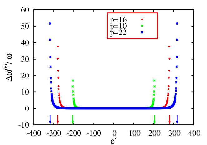
Figure 2: Relative difference between the exact result and the sixth–moment approximation $\Delta\omega^{(6)}/\omega=[\omega^{(6)}_{b}(p,\varepsilon^{\prime})-\omega_{b}(p,\varepsilon^{\prime})]/\omega_{b}(p,\varepsilon^{\prime})$ versus energy $\varepsilon^{\prime}$ for $b=51$ and several values of $p$. The spectral boundaries are indicated by the arrows on the abscissa.

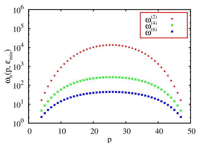
Figure 3: Second–, fourth–, and sixth–moment approximation to $\omega_{b}(p,\varepsilon)$ at the lower spectrum boundary $\varepsilon_{\mathrm{min}}=(1/2)p(p+1)$ versus $p$ for $b=51$.

We turn to the total level density $\omega_{u}(A,\varepsilon)$ of $A$ particles distributed over $u$ equally spaced single–particle states as a function of the dimensionless excitation energy $\varepsilon$. We have shown that $\omega_{u}(A,\varepsilon)$ has approximately Gaussian shape, with a peak at half the total excitation energy $(1/2)A(u+1)$. The original calculation of $\omega_{u}(A,\varepsilon)$ by Bethe Bet36 effectively also used a constant–spacing model but neglected the limitations due to finite particle number $A$ and finite number $u$ of single–particle states. With energy measured in units of the single–particle level spacing, the celebrated “Bethe formula” reads Bet36

$$\omega_{\rm Bethe}(\varepsilon)=\frac{1}{\varepsilon\sqrt{48}}\exp\{\pi\sqrt{2\varepsilon/3}\}\ .$$ (21)

We note that $\omega_{\rm Bethe}(\varepsilon)$ does not contain any adjustable parameters. The singularity at $\varepsilon=0$ is due to the Darwin–Fowler method. The ensuing approximation fails at and near $\varepsilon=0$. Beyond this domain the Bethe formula yields a monotonically rising function of excitation energy since the underlying counting method assumes that the number of available single–particle states is unbounded. Thus, there exists an excitation energy beyond which the Bethe formula exceeds $\omega_{u}(A,\varepsilon)$ by an ever growing amount. This fact was qualitatively pointed out in Ref. Wei64 . In Fig. 4 we compare $\omega_{\rm Bethe}(\varepsilon)$ with the exact calculation for $u=51$ and $A=41$ and with the sixth–moment approximation for $u=250$ and $A=200$ (for the latter parameters the exact density of state values are not available for the entire energy spectrum). The latter parameter set mimics, very roughly, a heavy nucleus. Comparison with the exact calculation shows that $\omega_{\rm Bethe}(\varepsilon)$ underestimates the level density below the crossing point of both curves. We have found this to be a systematic trend. Both parts of Fig. 4 clearly display the crossing point and the increasing discrepancy between $\omega_{\rm Bethe}(\varepsilon)$ and $\omega_{u}(A,\varepsilon)$ as $\varepsilon$ increases beyond this point.

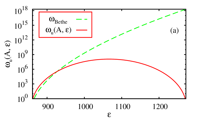
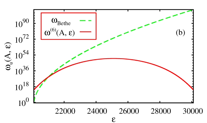
Figure 4: (a) Comparison of the exact level density $\omega_{u}(A,\varepsilon)$ for $u=51$, $A=41$ versus energy $\varepsilon$ with the Bethe formula (21). (b) The same for the sixth–moment approximation and $u=250$, $A=200$.

We interpret the data on the crossing points using the equilibrium distribution $n(\epsilon)=(1/A)\ 1/(1+\exp\{(\epsilon-A)/(kT)\}$ for $A$ Fermions at temperature $T$ with $kT\ll A$ and continuous single–particle energy $\epsilon$. With $kT\approx\sqrt{\varepsilon}$ where $\varepsilon$ is the total excitation energy of the many–body system, we find that the crossing points occur at an excitation energy $\varepsilon$ where the fraction of particles in states with energies $>u$ is of the order of a few percent. This is physically plausible. In a heavy nucleus this criterion corresponds to excitation energies around $200$ MeV.

With increasing excitation energy, the constant–spacing model becomes increasingly unrealistic. Indeed, the standard value Her92 $d\approx 13/A$ MeV for the average spacing of single–particle levels near the Fermi energy in medium–weight and heavy nuclei strongly underestimates the single–particle level spacing in low–lying shells. We recall that every subshell with spin $j$ contributes $(2j+1)$ states to $\rho_{p}(E)$ in Eq. (1). As a consequence, the number of states available for high–energy hole formation is smaller than predicted by the constant–spacing model. Therefore, the actual level density bends over more strongly with increasing excitation energy and terminates at a lower maximum energy than shown in Fig. 4, and the discrepancy with the Bethe formula is even bigger than presented there. The effect of an energy–dependent single–particle level density was previously addressed, for instance, in Refs. Bog92 ; Shl95 albeit under neglect of the exclusion principle.

To account for the shortcoming of the constant–spacing model we are in the process of improving our approach to calculate nuclear level densities. We divide the energy interval $U=B+F$ into several sections $l=1,2,\dots$ with constant level spacing $d_{l}$ each but with $d_{l}\neq d_{l^{\prime}}$ for $l\neq l^{\prime}$. Distributing $p$ particles in all possible ways over these sections, so that there are $p_{l}$ particles in section $l$, we can use our results for the constant–spacing model in each section separately. For a fixed distribution $\{p_{l}\}$ the level density is a convolution over a product of Gaussians. The total level density is the sum over all distributions $\{p_{l}\}$. We note that it will no longer be a symmetric function of energy.

VI Conclusions

Combining analytical and numerical methods, we have used a constant–spacing model for non–interacting spinless Fermions to develop a global approach to various nuclear level densities. This approach is viable also for large particle numbers and/or excitation energies where previous work runs into difficulties. As representative example we have displayed in detail the calculation of the particle density $\omega_{b}(p,\varepsilon)$ as a function of particle number $p$ and excitation energy $\varepsilon$. This function is symmetric about the center of the spectrum and, except for $p=1$ and $p=b-1$, displays a maximum at the center. It also possesses particle–hole symmetry. The shape of the boundaries of the spectrum and the two symmetries are responsible for the quasi–elliptical shape of the line of constant density in Fig. 1. With $\omega_{b}(p,\varepsilon)\approx 1$ at the boundaries of the spectrum, the value of $\omega_{b}(p,\varepsilon)$ at the center increases dramatically with increasing $b$ and $p\approx b/2$, reaching values near $10^{12}$ already for $b\approx 50$ (and even larger values as $b$ is further increased). The decrease by $12$ or more orders of magnitude from the center of the spectrum to the boundary poses a considerable challenge to viable analytical approximations. Guided by the fact that for $b\gg 1,p\gg 1$ $\omega_{b}(p,\varepsilon)$ becomes asymptotically a Gaussian function of energy, we have used analytical expressions for the low moments to determine a sixth–moment approximation to $\omega_{b}(p,\varepsilon)$. This approximation is excellent except for values of $p$ and $\varepsilon$ near the boundaries of the spectrum. These are indicated by the white dashed lines in Fig. 1. Here the numerical calculation of $\omega_{b}(p,\varepsilon)$ based on Eq. (4) is easy and fast. Combining both approaches we obtain a reliable and easy–to–handle method of calculating the overall nuclear level density and $p$–particle $h$–hole densities for medium–weight and heavy nuclei for all particle numbers and at all excitation energies. The results should be realistic except for limitations due to the underlying constant–spacing model. Because of shell effects the density of single–particle levels increases towards the Fermi energy, and this fact is not taken into account in the model. Work on a suitable generalization is under way. The Bethe formula is seen to fail beyond an excitation energy that amounts to approximately $200$ MeV in heavy nuclei.

References

- (1) Extreme Light Infrastructure, URL: www.extreme-light-infrastructure.eu 2012.
- (2) A. Di Piazza, C. Müller, K. Z. Hatsagortsyan and C. H. Keitel, Rev. Mod. Phys. in press (2012), eprint arXiv:1111.3886v2.
- (3) G. Mourou and T. Tajima, Science 331 (2011) 41.
- (4) H. A. Weidenmüller, Phys. Rev. Lett. 106 (2011) 122502.
- (5) H. A. Bethe, Phys. Rev. 50 (1936) 332.
- (6) T. Ericson, Adv. Phys. 9 (1960) 423.
- (7) M. Böhning, Nucl. Phys. A 152 (1970) 529.
- (8) F. C. Williams, Nucl. Phys. A 166 (1971) 231.
- (9) K. Stankiewicz, A. Marcinowski, and M. Herman, Nucl. Phys. A 435 (1985) 67.
- (10) P. Oblozinsky, Nucl. Phys. A 453 (1986) 127.
- (11) M. Herman, G. Reffo, and H. A. Weidenmüller, Nucl. Phys. A 536 (1992) 124.
- (12) C. Bloch, in Physique Nucleaire, Ecole d’Ete des Houches 1968, Gordon and Breach, New York, pp. 303 - 411.
- (13) G. Ghosh, R. W. Hasse, P. Schuck, and J. Winter, Phys. Rev. Lett. 50 (1983) 1250.
- (14) A. H. Blin, R. W. Hasse, B. Hiller, P. Schuck, and C. Yannouleas, Nucl. Phys. A 456 (1986) 109.
- (15) B. Lauritzen and G. Bertsch, Phys. Rev. C 39 (1989) 2412.
- (16) Y. Alhassid and B. Bush, Nucl. Phys,. A 565 (1993) 399.
- (17) N. Canosa, R. Rossignoli, and P. Ring, Phys. Rev. C 50 (1994) 2850.
- (18) S. Hilaire, J. P. Delaroche, and A. J. Koning, Nucl. Phys. A 632 (1998) 417.
- (19) B. V. Carlson and D. F. Mega, EPJ Web of Conferences 21 (2012) 09001.
- (20) H. A. Weidenmüller, Phys. Lett. 10 (1964) 331.
- (21) Ye. A. Bogila, V. M. Kolomietz, and A. I. Sanzhur, Z. Physik A 341 (1992) 373.
- (22) S. Shlomo, Ye. A. Bogila, V. M. Kolomietz, and A. I. Sanzhur, Z. Physik A 353 (1995) 27.