$k$-Connectivity in Random Key Graphs with Unreliable Links

Abstract

Random key graphs form a class of random intersection graphs and are naturally induced by the random key predistribution scheme of Eschenauer and Gligor for securing wireless sensor network (WSN) communications. Random key graphs have received much interest recently, owing in part to their wide applicability in various domains including recommender systems, social networks, secure sensor networks, clustering and classification analysis, and cryptanalysis to name a few. In this paper, we study connectivity properties of random key graphs in the presence of unreliable links. Unreliability of the edges are captured by independent Bernoulli random variables, rendering edges of the graph to be on or off independently from each other. The resulting model is an intersection of a random key graph and an Erdős–Rényi graph, and is expected to be useful in capturing various real-world networks; e.g., with secure WSN applications in mind, link unreliability can be attributed to harsh environmental conditions severely impairing transmissions. We present conditions on how to scale this model’s parameters so that i) the minimum node degree in the graph is at least $k$, and ii) the graph is $k$-connected, both with high probability as the number of nodes becomes large. The results are given in the form of zero-one laws with critical thresholds identified and shown to coincide for both graph properties. These findings improve the previous results by Rybarczyk on the $k$-connectivity of random key graphs (with reliable links), as well as the zero-one laws by Yağan on the $1$-connectivity of random key graphs with unreliable links.

I Introduction

Random key graphs have received significant interest recently with applications spanning key predistribution in secure wireless sensor networks (WSNs) [2, 5, 9, 8, 13], social networks [18, 41, 7], recommender systems [27], clustering and classification analysis [19, 4], cryptanalysis of hash functions [3], circuit design [35], and the modeling of epidemics [1] and “small-world” networks [38]. They belong to a larger class of random graphs known as random intersection graphs [2, 3, 5, 4, 6, 10, 28, 34, 14, 7, 35]; in fact, they are referred to as uniform random intersection graphs by some authors [2, 6, 3, 28, 32, 33, 34, 45, 46].

To fix the terminology, we will describe random key graphs in the context of secure WSNs, where they have originated from. Security is expected to be a key challenge in resource constrained sensor networks. A widely accepted solution for securing WSN communications is the random predistribution of cryptographic keys to sensor nodes, and utilization of symmetric-key encryption modes [17, 21, 31] to ensure message secrecy and authenticity. Among various key predistribution algorithms proposed to date, the original scheme by Eschenauer and Gligor (EG) [13] is still the most widely recognized one. According to the EG scheme, each of the $n$ sensors is assigned $K_{n}$ distinct keys that are selected uniformly at random from a key pool of size $P_{n}$. Two sensors can then securely communicate over an existing communication link if they have at least one key in common; i.e., if they share a common key. This notion of adjacency defines the random key graph, hereafter denoted by $G(n,K_{n},P_{n})$. For generality, $K_{n}$ and $P_{n}$ are assumed to scale with the number of nodes $n$, with the natural condition $1\leq K_{n}\leq P_{n}$ always imposed.

In this paper, we study connectivity properties of random key graphs in the presence of unreliable links. Unreliability of the edges are captured by independent Bernoulli random variables, rendering each edge of $G(n;K_{n},P_{n})$ to be on (with probability $p_{n}$) or off (with probability $1-p_{n}$) independently from all other edges. Put differently, we consider an Erdős–Rényi (ER) graph $G(n;p_{n})$ [11] on the same set of $n$ vertices, with edges appearing between any pair of vertices independently with probability $p_{n}$. A random key graph with unreliable links thus corresponds to the intersection of a random key graph and an ER graph. Hereafter, we denote this graph by $\mathbb{G}_{on}=G(n;K_{n},p_{n})\cap G(n;p_{n})$; see Section III for precise definitions.

Just like the random key graph, the $\mathbb{G}_{on}$ model can be used in various applications, particularly when links are expected to be unreliable. For example, in a secure WSN application, links might be unreliable due to wireless media of the communication, or due to physical obstacles and altering environmental conditions severally impairing the transmission. We refer the reader to [39] and [41] for two other applications of $\mathbb{G}_{on}$: i) secure connectivity of WSNs under an on-off channel model, and ii) large scale, distributed publish-subscribe services in online social networks, respectively.

The main goal of this paper to study $k$-connectivity of $\mathbb{G}_{on}$. A network (or graph) is said to be $k$-connected if for each pair of nodes there exist at least $k$ mutually disjoint paths connecting them. An equivalent definition of $k$-connectivity is that a network is $k$-connected if the network remains connected despite the failure of any $(k-1)$ nodes [29]; a network is said to be simply connected if it is $1$-connected. $k$-connectivity is a fundamental graph property and is important for various applications of random key graphs. For example, in a WSN application where sensor nodes operate autonomously and physically unprotected, $k$-connectivity provides communication security against an adversary that is able to compromise up to $k-1$ links by launching a sensor capture attack [8]; i.e., two sensors can communicate securely as long as at least one of the $k$ disjoint paths connecting them consists of links that are not compromised by the adversary. Also, $k$-connectivity improves resiliency against network disconnection due to battery depletion, in both normal mode of operation and under battery-depletion attacks [26]. Furthermore, it enables flexible communication-load balancing across multiple paths so that network energy consumption is distributed without penalizing any access path [15].

Our main contributions are zero-one laws for two related graph properties for $\mathbb{G}_{on}$: i) the minimum node degree being at least $k$, and ii) $k$-connectivity. Namely, we present conditions on how to scale the model parameters $K_{n}$, $P_{n}$, $p_{n}$ such that these properties hold with probability approaching to one and zero, respectively, as the number of nodes $n$ becomes large. Our main results also imply a zero-one law for $k$-connectivity in random key graph $G(n,K_{n},P_{n})$ (see Corollary 2), and the established result is shown to improve that given previously by Rybarczyk [32]; see Section IV-D for details. Moreover, for the $1$-connectivity of $\mathbb{G}_{on}$, we provide a stronger form of the zero-one law as compared to that given by Yağan [37]; see Section IV-D.

We organize the rest of the paper as follows: In Section II, we survey the relevant results from the literature, while in Section III we give a detailed description of the system model $\mathbb{G}_{on}$. The main results of the paper are presented (see Theorem 1) in Section IV, with a detailed discussion and comparisons with the existing results given in Section IV-D; also, in Section IV-E we provide numerical results that confirm Theorem 1. The basic ideas that pave the way in establishing Theorem 1 are given in Section V. Sections VI through VIII are devoted to establishing the zero-law part of Theorem 1, whereas the one-law of Theorem 1 is established in Sections IX through XIII. The paper is concluded in Section XIV, and some of the technical details are given in Appendix A-C.

II Related Work

Erdős and Rényi [11] and Gilbert [16] introduces the random graph $G(n,p)$, which is defined on $n$ nodes and there exists an edge between any two nodes with probability $p$ independently of all other edges. The probability $p$ can also be a function of $n$, in which case we refer to it as $p_{n}$. Throughout the paper, we refer to the random graph $G(n,p_{n})$ as an Erdős-Rényi (ER) graph following the convention in the literature.

Erdős and Rényi [11] prove that when $p_{n}$ is $\frac{\ln n+{\alpha_{n}}}{n}$, graph $G(n,p_{n})$ is asymptotically almost surely (a.a.s.) connected (resp., not connected) if $\lim_{n\to\infty}{\alpha_{n}}=+\infty$ (resp., $\lim_{n\to\infty}{\alpha_{n}}=-\infty$). In later work [12], they further explore $k$-connectivity [30] in $G(n,p_{n})$ and show that if $p_{n}=\frac{\ln n+{(k-1)}\ln\ln n+{\alpha_{n}}}{n}$, $G(n,p_{n})$ is a.a.s. $k$-connected (resp., not $k$-connected) if $\lim_{n\to\infty}{\alpha_{n}}=+\infty$ (resp., $\lim_{n\to\infty}{\alpha_{n}}=-\infty$).

Previous work [2, 32, 39] investigates the zero-one law for connectivity in random key graph $G(n,K_{n},P_{n})$, where $P_{n}$ and $K_{n}$ are the key pool size and the key ring size, respectively. Blackburn and Gerke [2] prove that if $K_{n}\geq 2$ and $P_{n}=\lfloor n^{\xi}\rfloor$, where $\xi$ is a positive constant, $G(n,K_{n},P_{n})$ is a.a.s. connected (resp., not connected) if $\liminf_{n\to+\infty}\frac{K_{n}^{2}n}{P_{n}\ln n}>1$ (resp., $\limsup_{n\to+\infty}\frac{K_{n}^{2}n}{P_{n}\ln n}<1$). Yağan and Makowski [39] demonstrate that if $K_{n}\geq 2$, $P_{n}=\Omega(n)$ and $\frac{K_{n}^{2}}{P_{n}}=\frac{\ln n+{\alpha_{n}}}{n}$, then $G(n,K_{n},P_{n})$ is a.a.s. connected (resp., not connected) if $\lim_{n\to\infty}{\alpha_{n}}=+\infty$ (resp., $\lim_{n\to\infty}{\alpha_{n}}=-\infty$). Rybarczyk [32] obtains a stronger result without requiring $P_{n}=\Omega(n)$. In particular, she derives the asymptotically exact probability of connectivity in $G(n,K_{n},P_{n})$ as follows: under $K_{n}\geq 2$, if the sequence $\alpha_{n}$ defined through $\frac{K_{n}^{2}}{P_{n}}=\frac{\ln n+{\alpha_{n}}}{n}$ has a limit $\alpha^{*}\in[-\infty,\infty]$, then the probability of $G(n,K_{n},P_{n})$ being connected approaches to $e^{-e^{-\alpha^{*}}}$ as $n\to\infty$. This asymptotically exact probability result is stronger than a zero–one law since the latter can be obtained by setting $\alpha^{*}$ as $\infty$ and $-\infty$ in the former. Rybarczyk also establishes [33, Remark 1, p. 5] a zero-one law for $k$-connectivity in $G(n,K_{n},P_{n})$ by showing the similarity between $G(n,K_{n},P_{n})$ and a random intersection graph [5] via a coupling argument. Specifically, she proves that if $P_{n}=\Theta(n^{\xi})$ for some $\xi>1$ and $\frac{K_{n}^{2}}{P_{n}}=\frac{\ln n+(k-1)\ln\ln n+{\alpha_{n}}}{n}$, then the $G(n,K_{n},P_{n})$ is a.a.s. $k$-connected (resp., not $k$-connected) if $\lim_{n\to\infty}{\alpha_{n}}=+\infty$ (resp., $\lim_{n\to\infty}{\alpha_{n}}=-\infty$).

Recently Yağan [37] gives a zero-one law for connectivity (i.e., 1-connectivity) in graph $G(n,K_{n},P_{n})\cap G(n,{p_{n}})$, which is the intersection of random key graph $G(n,K_{n},P_{n})$ and random graph $G(n,{p_{n}})$, and clearly is equivalent to our key graph $\mathbb{G}_{on}$; see Section III. Specifically, he proves that if $K_{n}\geq 2$, $P_{n}=\Omega(n)$ and ${p_{n}}\cdot\left[1-\frac{\binom{P_{n}-K_{n}}{K_{n}}}{\binom{P_{n}}{K_{n}}}\right]\sim\frac{c\ln n}{n}$ hold, and $\lim_{n\to\infty}({p_{n}}\ln n)$ exists, then graph $G(n,K_{n},P_{n})\cap G(n,{p_{n}})$ is asymptotically almost surely connected (resp., not connected) if $c>1$ (resp., $c<1$). A comparison of our results with the related work is given in Section IV-D.

After the submission of this paper, we have derived the asymptotically exact probability of $k$-connectivity in $G(n,K_{n},P_{n})$ [45] (resp., $\mathbb{G}_{on}$ [44]). Based on the proofs in this paper, we show i) that [45] under $P_{n}=\Omega(n)$, if the sequence $\alpha_{n}$ defined through $\frac{K_{n}^{2}}{P_{n}}=\frac{\ln n+{(k-1)}\ln\ln n+{\alpha_{n}}}{n}$ has a limit $\alpha^{*}\in[-\infty,\infty]$, then the probability of $G(n,K_{n},P_{n})$ being $k$-connected converges to $e^{-\frac{e^{-\alpha^{*}}}{(k-1)!}}$ as $n\to\infty$, and ii) that [44] under $P_{n}=\Omega(n)$ and $\frac{K_{n}}{P_{n}}=o(1)$, if the sequence $\alpha_{n}$ defined through ${p_{n}}\cdot\left[1-\frac{\binom{P_{n}-K_{n}}{K_{n}}}{\binom{P_{n}}{K_{n}}}\right]=\frac{\ln n+{(k-1)}\ln\ln n+{\alpha_{n}}}{n}$ has a limit $\alpha^{*}\in[-\infty,\infty]$, then the probability of $\mathbb{G}_{on}$ being $k$-connected converges to $e^{-\frac{e^{-\alpha^{*}}}{(k-1)!}}$ as $n\to\infty$.

III System Model $\mathbb{G}_{on}$

Consider a vertex set $\mathcal{V}=\{v_{1},v_{2},\ldots,v_{n}\}$. Each node $v_{i}\in\mathcal{V}$ is assigned a key ring $S_{i}$ that consists of $K_{n}$ distinct keys selected uniformly at random from a key pool $\mathcal{P}$ of size $P_{n}$. The random key graph $G(n,K_{n},P_{n})$ is defined on the vertex set $\mathcal{V}$ such that two distinct nodes $v_{i}$ and $v_{j}$ are adjacent, denoted $K_{ij}$, if their key rings have at least one key in common; i.e.,

$$K_{ij}=[S_{i}\cap S_{j}\neq\emptyset].$$

For distinct nodes $v_{x}$ and $v_{y}$, we let $S_{xy}$ denote the intersection of their key rings $S_{x}$ and $S_{y}$; i.e., $S_{xy}=S_{x}\cap S_{y}$.

Our main interest is to study random key graphs whose links are unreliable. In particular, we assume that each link is on with probability $p_{n}$, or off with probability $1-p_{n}$, independently from any other link. Namely, with $C_{ij}$ denoting the event that link between $v_{i}$ and $v_{j}$ is on, $\{C_{ij},~{}1\leq i<j\leq n\}$ are mutually independent such that

$${\mathbb{P}}\left[{C_{ij}}\right]=p_{n},\quad 1\leq i<j\leq n.$$ (1)

This unreliable link model can be represented [11] by an Erdős-Rényi (ER) graph $G(n,p_{n})$ on the vertices $\mathcal{V}$ such that there exists an edge between nodes $v_{i}$ and $v_{j}$ if the link between them is on; i.e., if the event $C_{ij}$ takes place.

Finally, the graph $\mathbb{G}_{on}(n,K_{n},P_{n},p_{n})$ is defined on the vertices $\mathcal{V}$ such that two distinct nodes $v_{i}$ and $v_{j}$ have an edge in between, denoted $E_{ij}$, if the events $K_{ij}$ and $C_{ij}$ take place at the same time. In other words, we have

$$E_{ij}=K_{ij}\cap C_{ij},\quad 1\leq i<j\leq n$$ (2)

so that

$$\mathbb{G}_{on}(n,K_{n},P_{n},p_{n})=G(n,K_{n},P_{n})\cap G(n,p_{n}).$$ (3)

Throughout, we simplify the notation by writing $\mathbb{G}_{on}$ instead of $\mathbb{G}_{on}(n,K_{n},P_{n},p_{n})$. Thus, our main model $\mathbb{G}_{on}$ is an intersection of a random key graph and an ER graph.

Throughout, we let $p_{s}(K_{n},P_{n})$ be the probability that the key rings of two distinct nodes share at least one key and let ${p_{e}}(K_{n},P_{n},p_{n})$ be the probability that there exists a link between two distinct nodes in $\mathbb{G}_{on}$. For simplicity, we write $p_{s}(K_{n},P_{n})$ as ${p_{s}}$ and write ${p_{e}}(K_{n},P_{n},p_{n})$ as ${p_{e}}$. Then for any two distinct nodes $v_{i}$ and $v_{j}$, we have

$$p_{s} :=\mathbb{P}[{K}_{ij}].$$ (4)

It is easy to derive $p_{s}$ in terms of $K_{n}$ and $P_{n}$ as shown in previous work [2, 32, 39]. In fact, we have

$$p_{s} =\mathbb{P}[S_{i}\cap S_{j}\neq\emptyset]=\begin{cases}1-\frac{\binom{P_{n}-K_{n}}{K_{n}}}{\binom{P_{n}}{K_{n}}},&\textrm{if }P_{n}\geq 2K_{n},\\ 1&\textrm{if }P_{n}<2K_{n}.\end{cases}$$ (5)

Given (2), the independence of the events ${C}_{ij}$ and ${K}_{ij}$ gives

$${p_{e}} :=\mathbb{P}[E_{ij}]=\mathbb{P}[{C}_{ij}]\cdot\mathbb{P}[{K}_{ij}]=p_{n}\cdot p_{s}$$ (6)

from (1) and (4). Substituting (5) into (6), we obtain

$${p_{e}} =p_{n}\cdot\left[1-\frac{\binom{P_{n}-K_{n}}{K_{n}}}{\binom{P_{n}}{K_{n}}}\right]\quad\textrm{if }P_{n}\geq 2K_{n}.$$ (7)

IV Main Results and Discussion

IV-A The Main Result

The main result of this paper, given below, establishes zero-one laws for $k$-connectivity and for the property that the minimum node degree is no less than $k$ in graph ${\mathbb{G}}_{on}$. Throughout this paper, $k$ is a positive integer and does not scale with $n$. Also, we let $\mathbb{N}$ (resp., $\mathbb{N}_{0}$) stand for the set of all non-negative (resp., positive) integers.

We refer to any pair of mappings $K,P:\mathbb{N}_{0}\rightarrow\mathbb{N}_{0}$ as a scaling as long as it satisfies the natural conditions

$$K_{n}\leq P_{n},\quad n=1,2,\ldots.$$ (8)

Similarly, any mapping $p:\mathbb{N}_{0}\rightarrow(0,1)$ defines a scaling.

Theorem 1.

Consider scalings $K,P:\mathbb{N}_{0}\rightarrow\mathbb{N}_{0}$, $p:\mathbb{N}_{0}\rightarrow(0,1)$ such that $K_{n}\geq 2$ for all $n$ sufficiently large. We define a sequence $\alpha:\mathbb{N}_{0}\rightarrow\mathbb{R}$ such that for any $n\in\mathbb{N}_{0}$, we have

$$p_{e} =\frac{\ln n+{(k-1)}\ln\ln n+{\alpha_{n}}}{n}.$$ (9)

The properties (a) and (b) below hold.

(a) If $\frac{K_{n}^{2}}{P_{n}}=o(1)$ and either there exists $\epsilon>0$ such that $p_{e}n>\epsilon$ holds for all $n$ sufficiently large or $\lim_{n\to\infty}p_{e}n=0$, then

$$\lim_{n\to\infty}\mathbb{P}\left[\mathbb{G}_{on}\textrm{ is }k\textrm{-connected}\hskip 2.0pt\right] =0\quad\textrm{if}~{}\lim_{n\to\infty}{\alpha_{n}}=-\infty,$$ (10)

and

$$\lim_{n\to\infty}\mathbb{P}\left[\begin{array}[]{c}\textrm{Minimum~{}node~{}degree}\\ \mbox{of ${\mathbb{G}}_{on}$ is no less than }k\end{array}\right] =0\>\>\>\textrm{if $\lim_{n\to\infty}{\alpha_{n}}=-\infty$}.$$ (13)

(b) If $P_{n}=\Omega(n)$ and $\frac{K_{n}}{P_{n}}=o(1)$, then

$$\lim_{n\to\infty}\mathbb{P}\left[\mathbb{G}_{on}\textrm{ is }k\textrm{-connected}\hskip 2.0pt\right] =1\>\>\textrm{if $\lim_{n\to\infty}{\alpha_{n}}=\infty$},$$ (14)

and

$$\lim_{n\to\infty}\mathbb{P}\left[\begin{array}[]{c}\textrm{Minimum~{}node~{}degree}\\ \mbox{of ${\mathbb{G}}_{on}$ is no less than }k\end{array}\right] =1\quad\textrm{if $\lim_{n\to\infty}{\alpha_{n}}=\infty$}.$$ (17)

Note that if we combine (10) and (14), we obtain the zero-one law for $k$-connectivity in $\mathbb{G}_{on}$, whereas combining (13) and (17) leads to the zero-one law for the minimum node degree. Therefore, Theorem 1 presents the zero-one laws of $k$-connectivity and the minimum node degree in graph $\mathbb{G}_{on}$. We also see from (9) that the critical scaling for both properties is given by $p_{e}=\frac{\ln n+(k-1)\ln\ln n}{n}$. The sequence $\alpha_{n}:\mathbb{N}_{0}\rightarrow\mathbb{R}$ defined through (9) therefore measures by how much the probability $p_{e}$ deviates from the critical scaling.

In case (b) of Theorem 1, the conditions $P_{n}=\Omega(n)$ and $\frac{K_{n}}{P_{n}}=o(1)$ indicate that the size of the key pool $P_{n}$ should grow at least linearly with the number of sensor nodes in the network, and should grow unboundedly with the size of each key ring. These conditions are enforced here merely for technical reasons, but they hold trivially in practical wireless sensor network applications [8, 9, 13]. Again, the condition $\frac{K_{n}^{2}}{P_{n}}=o(1)$ enforced for the zero-law in Theorem 1 is not a stringent one since the $P_{n}$ is expected to be several orders of magnitude larger than $K_{n}$. Finally, the condition that either $p_{e}n>\epsilon>0$ for all $n$ large or $\lim_{n\to\infty}p_{e}n=0$ is imposed to avoid degenerate situations. In most cases of interest it holds that $p_{e}n>\epsilon>0$ as otherwise the graph $\mathbb{G}_{on}$ becomes trivially disconnected. To see this, notice that $p_{e}n$ is an upper-bound on the expected degree of a node and that the expected number of edges in the graph is less than $p_{e}n^{2}$; yet, a connected graph on $n$ nodes must have at least $n-1$ edges.

IV-B Results with an approximation of probability $p_{s}$

An analog of Theorem 1 can be given with a simpler form of the scaling (9); i.e., with $p_{s}$ replaced by the more easily expressed quantity $K_{n}^{2}/P_{n}$, and hence with $p_{e}=p_{n}K_{n}^{2}/P_{n}$. In fact, in the case of random key graph $G(n,K_{n},P_{n})$ it is a common practice [2, 32, 39] to replace $p_{s}$ by $\frac{K_{n}^{2}}{P_{n}}$, owing to the fact [39] that

$$p_{s}\sim\frac{K_{n}^{2}}{P_{n}}\quad\textrm{if}\quad\frac{K_{n}^{2}}{P_{n}}=o(1).$$ (18)

However, when random key graph $G(n,K_{n},P_{n})$ is intersected with an ER graph $G(n,p_{n})$ (as in the case of $\mathbb{G}_{on}$) the simplification does not occur naturally (even under (18)), and as seen below, simpler forms of the zero-one laws are obtained at the expense of extra conditions enforced on the parameters $K_{n}$ and $P_{n}$.

Corollary 1.

Consider a positive integer $k$, and scalings $K,P:\mathbb{N}_{0}\rightarrow\mathbb{N}_{0}$, $p:\mathbb{N}_{0}\rightarrow(0,1)$ such that $K_{n}\geq 2$ for all $n$ sufficiently large. We define a sequence $\alpha:\mathbb{N}_{0}\rightarrow\mathbb{R}$ such that for any $n\in\mathbb{N}_{0}$, we have

$$p_{n}\cdot\frac{K_{n}^{2}}{P_{n}} =\frac{\ln n+{(k-1)}\ln\ln n+{\alpha_{n}}}{n}.$$ (19)

The properties (a) and (b) below hold.

(a) If $\frac{K_{n}^{2}}{P_{n}}=O(\frac{1}{\ln n})$ and $\lim_{n\to\infty}(\ln n+(k-1)\ln\ln n+\alpha_{n})=\infty$, then

$$\lim_{n\to\infty}\mathbb{P}\left[\mathbb{G}_{on}\textrm{ is }k\textrm{-connected}\hskip 2.0pt\right] =0\quad\textrm{if}~{}\lim_{n\to\infty}{\alpha_{n}}=-\infty,$$ (20)

and

$$\lim_{n\to\infty}\mathbb{P}\left[\begin{array}[]{c}\textrm{Minimum~{}node~{}degree}\\ \mbox{of ${\mathbb{G}}_{on}$ is no less than }k\end{array}\right] =0\>\>\>\textrm{if $\lim_{n\to\infty}{\alpha_{n}}=-\infty$}.$$ (23)

(b) If $P_{n}=\Omega(n)$ and $\frac{K_{n}^{2}}{P_{n}}=O(\frac{1}{\ln n})$, then

$$\lim_{n\to\infty}\mathbb{P}\left[\mathbb{G}_{on}\textrm{ is }k\textrm{-connected}\hskip 2.0pt\right] =1\>\>\textrm{if $\lim_{n\to\infty}{\alpha_{n}}=\infty$},$$ (24)

and

$$\lim_{n\to\infty}\mathbb{P}\left[\begin{array}[]{c}\textrm{Minimum~{}node~{}degree}\\ \mbox{of ${\mathbb{G}}_{on}$ is no less than }k\end{array}\right] =1\quad\textrm{if $\lim_{n\to\infty}{\alpha_{n}}=\infty$}.$$ (27)

A proof of Corollary 1 can be found in Section IV-F. Note that the condition $\frac{K_{n}^{2}}{P_{n}}=O(\frac{1}{\ln n})$ enforced in Corollary 1 implies both $\frac{K_{n}}{P_{n}}=o(1)$ and $\frac{K_{n}^{2}}{P_{n}}=o(1)$, and thus it is a stronger condition than those enforced in Theorem 1.

IV-C A Zero-One Law for $k$-Connectivity in Random Key Graphs

We now provide a useful corollary of Theorem 1 that gives a zero-one law for $k$-connectivity in the random key graph $G(n,K_{n},P_{n})$. As discussed in Section IV-D below, this result improves the one given implicitly by Rybarczyk [33].

Corollary 2.

Consider a positive integer $k$, and scalings $K,P:\mathbb{N}_{0}\rightarrow\mathbb{N}_{0}$ such that $K_{n}\geq 2$ for all $n$ sufficiently large. With $\alpha:\mathbb{N}_{0}\rightarrow\mathbb{R}$ given by

$$\frac{K_{n}^{2}}{P_{n}} =\frac{\ln n+{(k-1)}\ln\ln n+{\alpha_{n}}}{n},\quad n=1,2,\ldots,$$ (28)

the following two properties hold.

(a) If either there exists an $\epsilon>0$ such that $n\frac{K_{n}^{2}}{P_{n}}>\epsilon$ for all $n$ sufficiently large, or $\lim_{n\to\infty}n\frac{K_{n}^{2}}{P_{n}}=0$, then we have

$$\lim_{n\to\infty}\mathbb{P}\left[{G}(n,K_{n},P_{n})\textrm{ is }k\textrm{-connected}\hskip 2.0pt\right]=0~{}\textrm{if}~{}\lim_{n\to\infty}{\alpha_{n}}=-\infty.$$

(b) If $P_{n}=\Omega(n)$, then we have

$$\lim_{n\to\infty}\mathbb{P}\left[{G}(n,K_{n},P_{n})\textrm{ is }k\textrm{-connected}\hskip 2.0pt\right]=1\>\>\textrm{if}~{}\lim_{n\to\infty}{\alpha_{n}}=\infty.$$

A proof of Corollary 2 can be found in Section IV-G.

IV-D Discussion and Comparison with Related Results

As already noted in the literature [2, 11, 12, 32, 33, 39], Erdős-Rényi graph $G(n,p_{n})$ and random key graph $G(n,K_{n},P_{n})$ have similar $k$-connectivity properties when they are matched through their link probabilities; i.e. when $p_{n}=p_{s}$ with $p_{s}$ as defined in (5). In particular, Erdős and Rényi [12] showed that if $p_{n}=\frac{\ln n+(k-1)\ln\ln n+{\alpha_{n}}}{n}$, then $G(n,p_{n})$ is asymptotically almost surely $k$-connected (resp., not $k$-connected) if $\lim_{n\to\infty}{\alpha_{n}}=+\infty$ (resp., $\lim_{n\to\infty}{\alpha_{n}}=-\infty$). Similarly, Rybarczyk [33] has shown under some extra conditions (i.e., $P_{n}=\Theta(n^{\xi})$ with $\xi>1$) that if $p_{s}=\frac{\ln n+(k-1)\ln\ln n+{\alpha_{n}}}{n}$, then $G(n,K_{n},P_{n})$ is almost surely $k$-connected (resp., not $k$-connected) if $\lim_{n\to\infty}{\alpha_{n}}=+\infty$ (resp., $\lim_{n\to\infty}{\alpha_{n}}=-\infty$).

The analogy between these two results could be exploited to conjecture similar $k$-connectivity results for our system model $\mathbb{G}_{on}$. To see this, recall from (3) that

$${\mathbb{G}}_{on} =G(n,K_{n},P_{n})\cap G(n,{p_{n}}).$$ (29)

Since $G(n,K_{n},P_{n})$ and $G(n,p_{s})$ have similar $k$-connectivity properties, it would seem intuitive to replace $G(n,K_{n},P_{n})$ with $G(n,p_{s})$ in the above equation (29). Then, using

$${\mathbb{G}}_{on}\simeq G(n,p_{s})\cap G(n,{p_{n}})=G(n,p_{n}p_{s})=G(n,p_{e}),$$

we would automatically obtain Theorem 1 via the aforementioned results of Erdős and Rényi [12]. Unfortunately, such heuristic approaches can not be taken for granted as $G(n,K_{n},P_{n})\neq G(n,p_{s})$ in general. For instance, the two graphs are shown [40, 38] to exhibit quite different characteristics in terms of properties including clustering coefficient, number of triangles, etc. To this end, Theorem 1 formally validates the above intuition for the $k$-connectivity property, and it is worth mentioning that we establish Theorem 1 with a direct proof that does not rely on coupling arguments between random key graph and ER graph.

We now compare our results with those of Rybarczyk [33] for the $k$-connectivity of random key graph $G(n,K_{n},P_{n})$. As already noted, Rybarczyk [33, Remark 1, p. 5] has established an analog of Corollary 2, but under assumptions much stronger than ours. In particular, her result requires that $P_{n}=\Theta(n^{\xi})$ where $\xi>1$. In comparison, Corollary 2 established here enforces only that $P_{n}\geq\Omega(n)$, which is clearly a much weaker condition than $P_{n}=\Theta(n^{\xi})$ with $\xi>1$. More importantly, our condition $P_{n}\geq\Omega(n)$ requires (from (28)) only that $K_{n}=\Omega(\sqrt{\ln n})$ for the one-law to hold; i.e., for $\mathbb{G}_{on}$ to be $k$-connected. However, the condition $P_{n}=\Theta(n^{\xi})$ with $\xi>1$ enforced in [33] requires the key ring sizes to satisfy $K_{n}=\Omega(\sqrt{n^{\xi-1}\ln n})$ with $\xi-1>0$. This condition not only constitutes a much stronger requirement than $K_{n}=\Omega(\sqrt{\ln n})$, but it also renders the $k$-connectivity result given in [33] not applicable in the context of WSNs. This is because $K_{n}$ controls the number of keys kept in each sensor’s memory, and should be very small [13] due to limited memory and computational capability of sensor nodes; in general $K_{n}=O(\ln n)$ is accepted [9] as a reasonable bound on the key ring sizes.

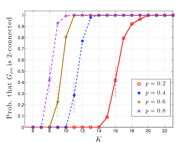
Figure 1: Empirical probability that $\mathbb{G}_{on}(n,K,P,p)$ is $2$-connected for $p=0.2$, $p=0.4$, $p=0.6$, $p=0.8$ with $n=2000$ and $P=10,000$. Vertical dashed lines stand for the critical threshold of $2$-connectivity asserted by Theorem 1.

Finally, we compare Theorem 1 with the zero-one law given by Yağan [37] for the $1$-connectivity of $\mathbb{G}_{on}$. As mentioned in Section II above, he shows that if

$$p_{e}\sim c\frac{\ln n}{n}=\frac{\ln n+(c-1)\ln n}{n}$$ (30)

then $\mathbb{G}_{on}$ is a.a.s. connected if $c>1$, and it is a.a.s. not connected if $c<1$. This was done under the additional conditions that $P_{n}=\Omega(n)$ (required only for the one-law) and that $\lim_{n\to\infty}p_{n}\ln n$ exists (required only for the zero-law). On the other hand, Theorem 1 given here establishes (by setting $k=1$) that, if

$$p_{e}=\frac{\ln n+\alpha_{n}}{n}$$ (31)

then $\mathbb{G}_{on}$ is a.a.s. connected if $\lim_{n\to\infty}\alpha_{n}=\infty$, and it is a.a.s. not connected if $\lim_{n\to\infty}\alpha_{n}=-\infty$. This result relies on the extra conditions $P_{n}=\Omega(n)$ and $\frac{K_{n}}{P_{n}}=o(1)$ for the one-law and on $\frac{K_{n}^{2}}{P_{n}}=o(1)$ for the zero-law.

Comparing (30) and (31), we see that our $1$-connectivity result for $\mathbb{G}_{on}$ is somewhat more fine-grained than Yağan’s [37]. This is because, a deviation of $\alpha_{n}=\pm\Omega(\ln n)$ is required to get the zero-one law in the form (30), whereas in our formulation (31), it suffices to have an unbounded deviation; e.g., even $\alpha_{n}=\pm\ln\ln\cdots\ln n$ will do. Put differently, we cover the case of $c=1$ in (30) (i.e., the case when $p_{e}\sim\frac{\ln n}{n}$) and show that $\mathbb{G}_{on}$ could be almost surely connected or not connected, depending on the limit of ${\alpha_{n}}$; in fact, if (30) holds with $c>1$, we see from Theorem 1 that $\mathbb{G}_{on}$ is not only $1$-connected but also $k$-connected for any $k=1,2,\ldots$. However, it is worth noting that the additional conditions assumed in [37] are weaker than those we enforce in Theorem 1 for $k=1$.

IV-E Numerical Results

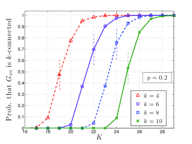
Figure 2: Empirical probability that $\mathbb{G}_{on}(n,K,P,p)$ is $k$-connected for $k=4,6,8$, and $10$. We take $n=2000$, $P=10,000$ and $p=0.2$. Vertical dashed lines stand for the critical threshold of $k$-connectivity asserted by Theorem 1.

We now present numerical results to check the validity of Theorem 1, particularly in the non-asymptotic regime. In all experiments, we fix the number of nodes at $n=2000$ and the size of the key pool at $P=10,000$. For Figure 1, we consider several different probabilities of links being on; specifically, we have $p=0.2,0.4,0.6,0.8$, while varying the parameter $K$ from $5$ to $23$; recall that $K$ stands for the number of keys per node. For Figure 2, we fix $p=0.2$ and vary $K$ from $16$ to $29$. For each parameter pair $(K,p)$, we generate $200$ independent samples of the graph $\mathbb{G}_{on}(n,K,P,p)$ and count the number of times (out of a possible 200) that the obtained graphs i) have minimum node degree no less than $k$ and ii) are $k$-connected, for $k=1,2,\ldots$. Dividing the counts by $200$, we obtain the (empirical) probabilities for the events of interest. In all cases, we observe that $\mathbb{G}_{on}$ is $k$-connected whenever its minimum node degree is no less than $k$, yielding the same empirical probability for both events. This confirms the asymptotic equivalence of the properties of $k$-connectivity and the minimum node degree being no less than $k$ in $\mathbb{G}_{on}$ as stated in Theorem 1.

Figure 1 plots the empirical probability of $2$-connectivity in $\mathbb{G}_{on}$ versus $K$ for different $p$ values, while Figure 2 depicts the empirical probability of $k$-connectivity in $\mathbb{G}_{on}$ versus $K$ for different $k$. For each curve, we also show the critical threshold of $k$-connectivity asserted by Theorem 1 (viz. (9)) by a vertical dashed line. Namely, the vertical dashed lines stand for the minimum integer value of $K$ that satisfies

$$p_{e}=p\cdot\left(1-{{{P-K}\choose K}\bigg{/}{P\choose K}}\right)>\frac{\ln n+\ln\ln n}{n}.$$ (32)

Even with $n=2000$, the threshold behavior in the probability of $k$-connectivity is evident; it transitions from zero to one with $K$ varying very slightly from a certain value that is close to the analytical prediction obtained from (32). Hence, we conclude that the experimentally observed thresholds of $k$-connectivity are in good agreement with our theoretical results.

IV-F A proof of Corollary 1

Consider $p_{n}$, $K_{n}$ and $P_{n}$ as in the statement of Corollary 1 such that (19) holds. As explained above, conditions $\frac{K_{n}}{P_{n}}=o(1)$ and $\frac{K_{n}^{2}}{P_{n}}=o(1)$ both hold. The proof is based on Theorem 1. Namely, we will show that if the sequence $\alpha^{\prime}:\mathbb{N}_{0}\rightarrow\mathbb{R}$ is defined such that

$$p_{e}=\frac{\ln n+{(k-1)}\ln\ln n+{\alpha^{\prime}_{n}}}{n}$$ (33)

for any $n\in\mathbb{N}_{0}$, then it holds that

$$\alpha^{\prime}_{n}=\alpha_{n}\pm O(1)$$ (34)

under the enforced assumptions. In view of $\lim_{n\to\infty}(\ln n+(k-1)\ln\ln n+\alpha_{n})=\infty$ and (34), we get $\lim_{n\to\infty}p_{e}n=\infty$ from (33). Thus, for any $\epsilon>0$, we have $p_{e}n>\epsilon$ for all $n$ sufficiently large. Hence, all the conditions enforced by Theorem 1 are met, and under (33) and (34), Corollary 1 follows from Theorem 1 since $\lim_{n\to\infty}{\alpha^{\prime}_{n}}=\pm\infty$ if $\lim_{n\to\infty}{\alpha_{n}}=\pm\infty$.

We now establish (34). First, as seen by the analysis given in Section V-B below, we can introduce the extra condition ${\alpha_{n}}=o(\ln n)$ in proving part (b) of Corollary 1; i.e., in proving the one-law under the condition $\lim_{n\to\infty}\alpha_{n}=\infty$. This yields $p_{n}\frac{K_{n}^{2}}{P_{n}}=O(\frac{\ln n}{n})$ under (19). Also, in the case $\lim_{n\to\infty}\alpha_{n}=-\infty$, we have $\alpha_{n}<0$ for all $n$ sufficiently large so that $p_{n}\frac{K_{n}^{2}}{P_{n}}=O(\frac{\ln n}{n})$. Now, in order to establish (34), we observe from part (a) of Lemma 8 that

$$p_{s} =\frac{K_{n}^{2}}{P_{n}}\pm O\left(\frac{K_{n}^{4}}{P_{n}^{2}}\right).$$ (35)

Then, from (35) and the fact that $p_{e}=p_{s}{p_{n}}$, we get

$$p_{e} ={p_{n}}\cdot\frac{K_{n}^{2}}{P_{n}}\pm{p_{n}}\cdot\frac{K_{n}^{2}}{P_{n}}\cdot O\left(\frac{K_{n}^{2}}{P_{n}}\right).$$ (36)

Substituting (19), $p_{n}\frac{K_{n}^{2}}{P_{n}}=O(\frac{\ln n}{n})$ and $\frac{K_{n}^{2}}{P_{n}}=O\left(\frac{1}{\ln n}\right)$ into (36), we find

$$p_{e} =\frac{\ln n+{(k-1)}\ln\ln n+{\alpha_{n}}\pm O(1)}{n}.$$ (37)

Comparing the above relation with (33), the desired conclusion (34) follows. $\blacksquare$

IV-G A proof of Corollary 2

We first establish the zero-law. Pick $K_{n}$, $P_{n}$ such that (28) holds with $\lim_{n\to\infty}\alpha_{n}=-\infty$. It is clear that we have $\alpha_{n}<0$ for all $n$ sufficiently large so that $\frac{K_{n}^{2}}{P_{n}}=O(\frac{\ln n}{n})=o(1)$. In view of (35) we thus get

$$p_{s}=\frac{\ln n+{(k-1)}\ln\ln n+{\alpha_{n}}\pm o(1)}{n},\quad n=1,2,\ldots$$

Let $p_{n}=1$ for all $n$. In this case, graph $\mathbb{G}_{on}$ becomes equivalent to $G(n,K_{n},P_{n})$ with

$$p_{e}=\frac{\ln n+{(k-1)}\ln\ln n+{\alpha_{n}}\pm o(1)}{n},\quad n=1,2,\ldots$$ (38)

From (38) and (28), we have $p_{e}n=n\frac{K_{n}^{2}}{P_{n}}\pm o(1)$ so that i) if there exists an $\epsilon>0$ such that $n\frac{K_{n}^{2}}{P_{n}}>\epsilon$, then there exists an $\epsilon^{\prime}>0$ such that $p_{e}n>\epsilon^{\prime}$ for all $n$ sufficiently large and ii) if $\lim_{n\to\infty}n\frac{K_{n}^{2}}{P_{n}}=0$, then $\lim_{n\to\infty}p_{e}n=0$. Thus, all the conditions enforced by part (a) of Theorem 1 are satisfied for the given $K_{n}$, $P_{n}$ and $p_{n}$. Comparing (38) with (9), we get $\lim_{n\to\infty}\alpha_{n}\pm o(1)=-\infty$ and the zero law $\lim_{n\to\infty}{\mathbb{P}}\left[{G(n,K_{n},P_{n})\textrm{ is }k\textrm{-connected}\hskip 2.0pt}\right]=0$ follows from (10) of Theorem 1.

We now establish the one-law. Pick $K_{n}$, $P_{n}$ such that (28) holds with $\lim_{n\to\infty}\alpha_{n}=+\infty$, $P_{n}=\Omega(n)$ and $K_{n}\geq 2$ for all $n$ sufficiently large. In view of [39, Lemma 6.1], there exists $\tilde{K}_{n}$, $\tilde{P}_{n}$ such that $\tilde{K}_{n}\geq 2$ for all $n$ sufficiently large,

$$\tilde{K}_{n}\leq K_{n}\quad\textrm{and}\quad\tilde{P}_{n}=P_{n},\quad n=1,2,\ldots,$$

and

$$\frac{\tilde{K}_{n}^{2}}{\tilde{P}_{n}}=\frac{\ln n+{(k-1)}\ln\ln n+{\tilde{\alpha}_{n}}}{n},\quad n=1,2,\ldots,$$ (39)

with

$$\tilde{\alpha}_{n}=O(\ln n)\quad\textrm{and}\quad\lim_{n\to\infty}\tilde{\alpha}_{n}=\infty.$$

By an easy coupling argument, it is easy to check that

$$\mathbb{P}\left[{G}(n,\tilde{K}_{n},\tilde{P}_{n})\textrm{ is }k\textrm{-connected}\hskip 2.0pt\right]$$

$$\leq\mathbb{P}\left[{G}(n,K_{n},P_{n})\textrm{ is }k\textrm{-connected}\hskip 2.0pt\right].$$

Therefore, the one-law proof will be completed upon showing

$$\lim_{n\to\infty}{\mathbb{P}}\left[{G(n,\tilde{K}_{n},\tilde{P}_{n})\textrm{ is }k\textrm{-connected}\hskip 2.0pt}\right] =1.$$

Under (39) we have $\frac{\tilde{K}_{n}^{2}}{\tilde{P}_{n}}=O(\frac{\ln n}{n})=o(1)$ since $\tilde{\alpha}_{n}=O(\ln n)$. It also follows that $\frac{\tilde{K}_{n}}{\tilde{P}_{n}}=o(1)$. In view of (35), we get

$$\tilde{p_{s}}=\frac{\ln n+{(k-1)}\ln\ln n+{\tilde{\alpha}_{n}}\pm o(1)}{n},\quad n=1,2,\ldots,$$

and with $p_{n}=1$ for all $n$ sufficiently large, we obtain

$$\tilde{p_{e}}=\frac{\ln n+{(k-1)}\ln\ln n+{\tilde{\alpha}_{n}}\pm o(1)}{n},\quad n=1,2,\ldots,$$

It is clear that $\lim_{n\to\infty}\tilde{\alpha}_{n}\pm o(1)=\infty$. Thus, we get the desired one-law by applying (14) of Theorem 1. $\blacksquare$

V Basic Ideas for Proving Theorem 1

V-A $k$-Connectivity vs. Minimum Node Degree

It is easy to see that if a graph $G$ is $k$-connected, then the minimum node degree of $G$ is at least $k$ [29]. Therefore, we have

$$\left[{G}\textrm{ is }k\textrm{-connected}\hskip 2.0pt\right]\subseteq\left[\begin{array}[]{c}\textrm{Minimum~{}node~{}degree}\\ \mbox{of ${G}$ is no less than }k\end{array}\right]$$

and the inequality

$$\mathbb{P}\left[{G}\textrm{ is }k\textrm{-connected}\hskip 2.0pt\right]\leq\mathbb{P}\left[\begin{array}[]{c}\textrm{Minimum~{}node~{}degree}\\ \mbox{of ${G}$ is no less than }k\end{array}\right]$$

follows immediately.

It is now clear that (13) implies (10) and (14) implies (17). Thus, in order to prove Theorem 1, we only need to show (13) under the conditions of case (a), and (14) under the conditions of case (b).

V-B Confining $\alpha_{n}$

As seen in Section V-A, Theorem 1 will follow if we show (13) and (14) under the appropriate conditions. In this subsection, we show that the extra condition ${\alpha_{n}}=o(\ln n)$ can be introduced in the proof of (14). Namely, we will show that

part (b) of Theorem 1 under $$\alpha_{n}=o(\ln n)$$

$$\Rightarrow\textrm{part (b) of Theorem \ref{thm:unreliableq1}}\hskip 56.9055pt$$ (40)

We write $\mathbb{G}_{{on}}$ as $\mathbb{G}_{{on}}(n,K_{n},P_{n},p_{n})$ and remember that given $K_{n}$, $P_{n}$ and $p_{n}$, one can determine $\alpha_{n}$ from (9); just use (7).

Assume that part (b) of Theorem 1 holds under the extra condition $\alpha_{n}=o(\ln n)$. The desired result (40) will follow if we establish

$$\lim_{n\to\infty}\mathbb{P}\left[{G}(n,\tilde{K}_{n},\tilde{P}_{n},\tilde{p}_{n})\textrm{ is }k\textrm{-connected}\hskip 2.0pt\right]=1$$ (41)

for any $\tilde{K}_{n}$, $\tilde{P}_{n}$ and $\tilde{p}_{n}$ such that $\frac{\tilde{K}_{n}}{\tilde{P}_{n}}=o(1)$, $\tilde{P}_{n}=\Omega(n)$, and

$$\tilde{p}_{e}=\frac{\ln n+(k-1)\ln\ln n+\tilde{\alpha}_{n}}{n}$$ (42)

holds with $\lim_{n\to\infty}{\tilde{\alpha}_{n}}=+\infty$. We will prove (41) by a coupling argument. Namely, we will show that there exist scalings $\hat{K}_{n}$, $\hat{P}_{n}$ and $\hat{p}_{n}$ such that

$$\frac{\hat{K}_{n}}{\hat{P}_{n}}=o(1)\quad\textrm{and}\quad\hat{P}_{n}=\Omega(n)$$ (43)

and

$$\hat{p}_{e}=\frac{\ln n+(k-1)\ln\ln n+\hat{\alpha}_{n}}{n}$$ (44)

with

$$\hat{\alpha}_{n}=o(\ln n)\quad\textrm{and}\quad\lim_{n\to\infty}\hat{\alpha}_{n}=\infty,$$ (45)

and that we have

$$\mathbb{P}[\mathbb{G}_{{on}}(n,\tilde{K}_{n},\tilde{P}_{n},{\tilde{p}_{n}})\textrm{ is $k$-connected }]$$

$$\geq\mathbb{P}[\mathbb{G}_{{on}}(n,\hat{K}_{n},\hat{P}_{n},\hat{p}_{n})\textrm{ is $k$-connected }].$$ (46)

Notice that $\hat{K}_{n}$, $\hat{P}_{n}$ and $\hat{p}_{n}$ satisfy all the conditions enforced by part (b) of Theorem 1 together with the extra condition $\hat{\alpha}_{n}=o(\ln n)$. Thus, we get

$$\lim_{n\to\infty}\mathbb{P}[\mathbb{G}_{{on}}(n,\hat{K}_{n},\hat{P}_{n},\hat{p}_{n})\textrm{ is $k$-connected }]=1$$ (47)

by the initial assumption, and (41) follows immediately from (46) and (47). Therefore, given any $\tilde{K}_{n}$, $\tilde{P}_{n}$ and $\tilde{p}_{n}$ as stated above, if we can show the existence of $\hat{K}_{n}$, $\hat{P}_{n}$ and $\hat{p}_{n}$ that satisfy (43)-(46), then the desired conclusion (40) will follow.

We now establish the existence of $\hat{K}_{n}$, $\hat{P}_{n}$ and $\hat{p}_{n}$ that satisfy (43)-(46). Let $\hat{P}_{n}=\tilde{P}_{n}$ and $\hat{K}_{n}=\tilde{K}_{n}$ so that (43) is satisfied automatically. Let $\hat{\alpha}_{n}=\min\left\{\tilde{\alpha}_{n},\ln\ln n\right\}$. Hence, we have $\hat{\alpha}_{n}\leq\tilde{\alpha}_{n}$, $\hat{\alpha}_{n}=o(\ln n)$ and $\lim_{n\to\infty}{\hat{\alpha}_{n}}=+\infty$ so that (45) is also satisfied. The remaining parameter $\hat{p}_{n}$ will be defined through

$$\hat{p}_{n}\cdot\left[1-\frac{\binom{\hat{P}_{n}-\hat{K}_{n}}{\hat{K}_{n}}}{\binom{\hat{P}_{n}}{\hat{K}_{n}}}\right]=\frac{\ln n+(k-1)\ln\ln n+\hat{\alpha}_{n}}{n}$$ (48)

so that $\hat{p}_{e}=\hat{p}_{n}\cdot\left[1-\frac{\binom{\hat{P}_{n}-\hat{K}_{n}}{\hat{K}_{n}}}{\binom{\hat{P}_{n}}{\hat{K}_{n}}}\right]$ satisfies (44). Thus, it remains to establish (46).

Comparing (48) with (42), it follows that $\hat{p}_{n}\leq\tilde{p}_{n}$ since $\hat{K}_{n}=\tilde{K}_{n}$, $\hat{P}_{n}=\tilde{P}_{n}$ and $\hat{\alpha}_{n}\leq\tilde{\alpha}_{n}$. Consider graphs $\mathbb{G}_{{on}}(n,\tilde{K}_{n},\tilde{P}_{n},\tilde{p}_{n})$, $\mathbb{G}_{{on}}(n,\tilde{K}_{n},\tilde{P}_{n},{\hat{p}_{n}})$ that have the same number of nodes $n$, the same key ring size $\tilde{K}_{n}$ and the same key pool size $\tilde{P}_{n}$, but have different probabilities $\tilde{p}_{n}$ and $\hat{p}_{n}$ for a link to be on. We will show that there exists a coupling such that $\mathbb{G}_{{on}}(n,\tilde{K}_{n},\tilde{P}_{n},{\hat{p}_{n}})$ is a spanning subgraph of $\mathbb{G}_{{on}}(n,\tilde{K}_{n},\tilde{P}_{n},{\tilde{p}_{n}})$ so that, as shown by Rybarczyk [33, pp. 7], we have

$$\mathbb{P}[\mathbb{G}_{{on}}(n,\tilde{K}_{n},\tilde{P}_{n},{\hat{p}_{n}})\textrm{ has property }\mathscr{P}]$$

$$\leq\mathbb{P}[\mathbb{G}_{{on}}(n,\tilde{K}_{n},\tilde{P}_{n},\tilde{p}_{n})\textrm{ has property }\mathscr{P}].$$ (49)

for any monotone increasing graph property $\mathscr{P}$. The properties of being $k$-connected and having a minimum node degree of at least $k$ can easily be seen to be monotone increasing graph properties. Therefore, (46) will follow immediately (with $\hat{K}_{n}=\tilde{K}_{n}$ and $\hat{P}_{n}=\tilde{P}_{n}$) if (49) holds.

We now give the coupling argument that leads to (49). As seen from (3), $\mathbb{G}_{on}$ is the intersection of a random key graph $G(n,K_{n},P_{n})$ and an Erdős-Rényi graph $G(n,{p_{n}})$. Using graph coupling, we use the same random key graph $G(n,\tilde{K}_{n},\tilde{P}_{n})$ to help construct both $\mathbb{G}_{on}(n,\tilde{K}_{n},\tilde{P}_{n},{\tilde{p}_{n}})$ and $\mathbb{G}_{on}(n,\tilde{K}_{n},\tilde{P}_{n},{\hat{p}_{n}})$. Then we have

$$\mathbb{G}_{on}(n,\tilde{K}_{n},\tilde{P}_{n},{\tilde{p}_{n}}) =G(n,\tilde{K}_{n},\tilde{P}_{n})\cap G(n,{\tilde{p}_{n}})$$ (50)

$$\mathbb{G}_{on}(n,\tilde{K}_{n},\tilde{P}_{n},{\hat{p}_{n}}) =G(n,\tilde{K}_{n},\tilde{P}_{n})\cap G(n,\hat{p}_{n}).$$ (51)

Since ${\hat{p}_{n}}\leq{\tilde{p}_{n}}$, we couple $G(n,\hat{p}_{n})$ and $G(n,\tilde{p}_{n})$ in the following manner. Pick independent Erdős-Rényi graphs $G(n,{\hat{p}_{n}/\tilde{p}_{n}})$ and $G(n,\tilde{p}_{n})$ on the same vertex set. It is clear that the intersection $G(n,{\hat{p}_{n}/\tilde{p}_{n}})\cap G(n,\tilde{p}_{n})$ will still be an Erdős-Rényi graph (due to independence) with an edge probability given by $\tilde{p}_{n}\cdot\frac{\hat{p}_{n}}{\tilde{p}_{n}}=\hat{p}_{n}$. In other words, we have $G(n,{\hat{p}_{n}/\tilde{p}_{n}})\cap G(n,\tilde{p}_{n})=G(n,\hat{p}_{n})$. Consequently, under this coupling, $G(n,{\hat{p}_{n}})$ is a spanning subgraph of $G(n,\tilde{p}_{n})$. Then from (50) and (51), $\mathbb{G}_{on}(n,\tilde{K}_{n},\tilde{P}_{n},\hat{p}_{n})$ is a spanning subgraph of $\mathbb{G}_{on}(n,\tilde{K}_{n},\tilde{P}_{n},\tilde{p}_{n})$ and (49) follows.

V-C The Method of First and Second Moments

The following fact is based on the method of the first and second moments and will be useful in deriving zero-one laws for the minimum node degree of a graph. We use $\mathbb{E}[\cdot]$ to denote the expectation operator.

Fact 1.

For any graph $G$ with $n$ nodes, let $X_{\ell}$ be the number of nodes having degree $\ell$ in $G$, where $\ell=0,1,\ldots,n-1$; and let $\delta$ be the minimum node degree of $G$. Then the following three properties hold for any positive integer $k$.

(a) For any non-negative integer $\ell$, if $\mathbb{E}[X_{\ell}]=o(1)$, then

$$\lim_{n\rightarrow\infty}{\mathbb{P}}\left[{\delta=\ell}\right]=0.$$ (52)

(b) If (52) holds for $\ell=0,1,\ldots,{k-1}$, then

$$\lim_{n\to\infty}\mathbb{P}[\delta\geq k] =1.$$

(c) If $\mathbb{E}\left[{\big{(}X_{\ell}\big{)}}^{2}\right]\sim\big{\{}\mathbb{E}\big{[}X_{\ell}\big{]}\big{\}}^{2}$ and $\mathbb{E}\big{[}X_{\ell}\big{]}\to+\infty$ as $n\to\infty$ hold for some $\ell=0,1,\ldots,k-1$, then

$$\lim_{n\to\infty}\mathbb{P}[\delta\geq k] =0.$$

A proof of Fact 1 is given in Appendix B-A.

V-D Useful Notation for Graph $\mathbb{G}_{on}$

We collect in this section some notation that will be used throughout. For any event $A$, we let $\overline{A}$ be the complement of $A$. Also, for sets $S_{a}$ and $S_{b}$, the relative complement of $S_{a}$ in $S_{b}$ is given by $S_{a}\setminus S_{b}$.

In graph $\mathbb{G}_{on}$, for each node $v_{i}\in\mathcal{V}$, we define $N_{i}$ as the set of neighbors of node $v_{i}$. For any two distinct nodes $v_{x}$ and $v_{y}$, there are $(n-2)$ nodes other than $v_{x}$ and $v_{y}$ in graph $\mathbb{G}_{on}$. These $(n-2)$ nodes can be split into the four sets $N_{xy}$, $N_{x\overline{y}}$, $N_{\overline{x}y}$ and $N_{\overline{x}\hskip 1.5pt\overline{y}}$ as follows. Let $N_{xy}$ be the set of nodes that are neighbors of both $v_{x}$ and $v_{y}$; i.e., $N_{xy}=N_{x}\cap N_{y}$. Let $N_{x\overline{y}}$ denote the set of nodes in $\mathcal{V}\setminus\{v_{x},v_{y}\}$ that are neighbors of $v_{x}$, but are not neighbors of $v_{y}$. Similarly, $N_{\overline{x}y}$ is defined as the set of nodes in $\mathcal{V}\setminus\{v_{x},v_{y}\}$ that are not neighbors of $v_{x}$, but are neighbors of $v_{y}$. Finally, $N_{\overline{x}\hskip 1.5pt\overline{y}}$ is the set of nodes in $\mathcal{V}\setminus\{v_{x},v_{y}\}$ that are not connected to either $v_{x}$ or $v_{y}$.

For any three distinct nodes $v_{x},v_{y}$ and $v_{j}$, recalling that $E_{xj}$ (resp., $E_{yj}$) is the event that there exists a link between nodes $v_{x}$ (resp., $v_{y}$) and $v_{j}$, we define

$$E_{{x}j\cap{y}j} :=E_{{x}j}\cap E_{{y}j},\textrm{~{}~{}~{}~{}~{}~{}}E_{{x}j\cap\overline{{{y}j}}}:=E_{{x}j}\cap\overline{E_{{y}j}},$$

$$E_{\overline{{x}j}\cap{y}j} :=\overline{E_{{x}j}}\cap E_{{y}j},\textrm{ and }E_{\overline{{x}j}\cap\overline{{{y}j}}}:=\overline{E_{{x}j}}\cap\overline{E_{{y}j}}.$$

In graph $\mathbb{G}_{on}$, for any non-negative integer $\ell$, let $X_{\ell}$ be the number of nodes having degree $\ell$; let $D_{x,\ell}$ be the event that node $v_{x}$ has degree $\ell$. We define $\delta$ as the minimum node degree of graph $\mathbb{G}_{on}$, and define $\kappa$ as the connectivity of graph $\mathbb{G}_{on}$. The connectivity of a graph is defined as the minimum number of nodes whose deletion renders the graph disconnected; thus, a graph is $k$-connected if and only if its connectivity is at least $k$. Finally, a graph is said to be simply connected if its connectivity is at least $1$, i.e., if it is $1$-connected.

VI Establishing (13) (The Zero-Law for the Minimum Node Degree in $\mathbb{G}_{on}$)

Our main goal in this section is to establish (13) under the following conditions:

$$(\ref{eqn:unreliable}),K_{n}\geq 2\textrm{ for all $n$ sufficiently large },\frac{K_{n}^{2}}{P_{n}}=o(1)$$ (53)

$$\lim_{n\to+\infty}{\alpha_{n}}=-\infty\textrm{ and }p_{e}n>\epsilon>0~{}\textrm{or}~{}{\lim_{n\to\infty}p_{e}n}=0.$$ (54)

From property (c) of Fact 1, we see that the proof will be completed if we demonstrate the following two results under the conditions (53) and (54):

$$\lim_{n\to\infty}\mathbb{E}\big{[}X_{\ell}\big{]} =+\infty,$$ (55)

and

$$\mathbb{E}\left[{\big{(}X_{\ell}\big{)}}^{2}\right] \sim\big{\{}\mathbb{E}\big{[}X_{\ell}\big{]}\big{\}}^{2}.$$ (56)

for some $\ell=0,1,\ldots,k-1$.

The first step in establishing (55) and (56) is to compute the moments $\mathbb{E}\left[X_{\ell}\right]$ and $\mathbb{E}\left[{\left(X_{\ell}\right)}^{2}\right]$. This step is taken in the next Lemma. Recall that in graph $\mathbb{G}_{on}$, $X_{\ell}$ stands for the number of nodes with degree $\ell$ for each $\ell=0,1,\ldots$. Also, $D_{x,\ell}$ is the event that node $v_{x}$ has degree $\ell$ for each $x=1,2,\ldots,n$.

Lemma 1.

In $\mathbb{G}_{on}$, for any non-negative integer $\ell$ and any two distinct nodes $v_{x}$ and $v_{y}$, we have

$$\mathbb{E}\big{[}X_{\ell}\big{]} =n\mathbb{P}\left[D_{x,\ell}\right],$$ (57)

$$\mathbb{E}\left[{\big{(}X_{\ell}\big{)}}^{2}\right] =n\mathbb{P}\left[D_{x,\ell}\right]+n(n-1)\mathbb{P}\left[D_{x,\ell}\textstyle{\bigcap}D_{y,\ell}\right].$$ (58)

Lemma 1 follows from the exchangeability of the indicator random variables $\{\mathbf{1}[D_{i,\ell}];i=1,\ldots,n\}$ upon writing $X_{\ell}=\sum_{i=1}^{n}\mathbf{1}[D_{i,\ell}]$. Interested reader is referred to the full version [41] for details.

In view of (57), we will obtain (55) once we show that

$$\lim_{n\to+\infty}\left(n\mathbb{P}\left[D_{x,\ell}\right]\right) =+\infty.$$ (59)

under (53) and (54). Also, from (57) and (58), we get

$$\frac{\mathbb{E}\left[{\big{(}X_{\ell}\big{)}}^{2}\right]}{\big{\{}\mathbb{E}\big{[}X_{\ell}\big{]}\big{\}}^{2}} =\frac{1}{n\mathbb{P}\left[D_{x,\ell}\right]}+\frac{n-1}{n}\cdot\frac{\mathbb{P}\left[D_{x,\ell}\textstyle{\bigcap}D_{y,\ell}\right]}{\big{\{}\mathbb{P}\left[D_{x,\ell}\right]\big{\}}^{2}}.$$ (60)

Thus, (56) will follow upon showing (59) and

$$\mathbb{P}\left[D_{x,\ell}\textstyle{\bigcap}D_{y,\ell}\right] \sim\big{\{}\mathbb{P}\left[D_{x,\ell}\right]\big{\}}^{2}$$ (61)

for some $\ell=0,1,\ldots,k-1$ under (53) and (54).

We establish (59) and (61) from of the following two results.

Lemma 2.

If ${p_{e}}=o\left(\frac{1}{\sqrt{n}}\right)$, then for any non-negative integer constant $\ell$ and any node $v_{x}$,

$$\mathbb{P}\left[D_{x,\ell}\right] \sim\left(\ell!\right)^{-1}\left({p_{e}}n\right)^{\ell}e^{-{p_{e}}n}.$$ (62)

A proof of Lemma 2 is given in Appendix C-A.

Lemma 3.

Let $p_{s}=o(1)$, $K_{n}\geq 2$ for all $n$ sufficiently large, $p_{e}=\frac{\ln n+(k-1)\ln\ln n+\alpha_{n}}{n}$ with $\lim_{n\to\infty}\alpha_{n}=-\infty$. Then, properties (a) and (b) below hold.

(a) If there exist an $\epsilon>0$ such that $p_{e}n>\epsilon$ for all $n$ sufficiently large, then for any non-negative integer constant $\ell$ and any two distinct nodes $v_{x}$ and $v_{y}$, we have

$$\mathbb{P}\left[D_{x,{\ell}}\cap D_{y,{\ell}}\right] \sim({\ell}!)^{-2}\left({p_{e}}n\right)^{2\ell}e^{-2{p_{e}}n}.$$ (63)

(b) For any two distinct nodes $v_{x}$ and $v_{y}$, we have

$$\mathbb{P}\left[D_{x,{0}}\cap D_{y,{0}}\right] \sim e^{-2{p_{e}}n}.$$ (64)

Proof.  Recalling that $E_{{x}{y}}$ is the event that nodes $v_{x}$ and $v_{y}$ are adjacent, we have

$$\mathbb{P}\left[D_{x,{\ell}}\cap D_{y,{\ell}}\right]$$

$$=\mathbb{P}[D_{x,{\ell}}\cap D_{y,{\ell}}\cap\overline{E_{{x}{y}}}]+\mathbb{P}[D_{x,{\ell}}\cap D_{y,{\ell}}\cap E_{{x}{y}}].$$ (65)

Thus, Lemma 3 will follow from the following two results.

Proposition 1.

Let $p_{s}=o(1)$, $K_{n}\geq 2$ for all $n$ sufficiently large and $p_{e}=\frac{\ln n+(k-1)\ln\ln n+\alpha_{n}}{n}$ with $\lim_{n\to\infty}\alpha_{n}=-\infty$. Then, the following two properties hold.

(a) If there exist an $\epsilon>0$ such that $p_{e}n>\epsilon$ for all $n$ sufficiently large, then for any non-negative integer constant $\ell$, we have

$$\mathbb{P}[D_{x,{\ell}}\cap D_{y,{\ell}}\cap\overline{E_{{x}{y}}}] \sim({\ell}!)^{-2}\left({p_{e}}n\right)^{2\ell}e^{-2{p_{e}}n}.$$ (66)

(b) We have

$$\mathbb{P}[D_{x,{0}}\cap D_{y,{0}}\cap\overline{E_{{x}{y}}}] \sim e^{-2{p_{e}}n}.$$ (67)

Proposition 2.

Let $p_{s}=o(1)$, $K_{n}\geq 2$ for all $n$ sufficiently large and $p_{e}=\frac{\ln n+(k-1)\ln\ln n+\alpha_{n}}{n}$ with $\lim_{n\to\infty}\alpha_{n}=-\infty$. If there exists an $\epsilon>0$ such that $p_{e}n>\epsilon$ for all $n$ sufficiently large, then for any positive integer constant $\ell$, we have

$$\mathbb{P}[D_{x,{\ell}}\cap D_{y,{\ell}}\cap E_{{x}{y}}] =o\left(\mathbb{P}[D_{x,{\ell}}\cap D_{y,{\ell}}\cap\overline{E_{{x}{y}}}]\right).$$ (68)

Propositions 1 and 2 are established in Section VII and Section VIII, respectively. Now, we complete the proof of Lemma 3. Under the condition $p_{e}n>\epsilon>0$, (63) follows from (66) and (68) in view of (65). For $\ell=0$, we obtain (64) by using (67) in (65) and noting that $\mathbb{P}[D_{x,{0}}\cap D_{y,{0}}\cap{E_{{x}{y}}}]=0$ always holds; it is not possible for nodes $v_{x}$ and $v_{y}$ to have degree zero and yet to have an edge in between.  

We now complete the proof of (59) and (61) under (53) and (54). First, in view of (9) and the condition $\lim_{n\to\infty}{\alpha_{n}}=-\infty$, we obtain ${p_{e}}\leq\frac{\ln n+(k-1)\ln\ln n}{n}$ for all $n$ sufficiently large. Thus, ${p_{e}}=o\big{(}\frac{1}{\sqrt{n}}\big{)}$, and we use Lemma 2 to get

$$n\mathbb{P}\left[D_{x,\ell}\right] \sim n\cdot\left(\ell!\right)^{-1}\left({p_{e}}n\right)^{\ell}e^{-{p_{e}}n}$$ (69)

for each $\ell=0,1,\ldots$. The proof will be given in two steps. First, in the case where there exists an $\epsilon>0$ such that $p_{e}n>\epsilon$ for all $n$ sufficiently large, we will establish (59) and (61) for $\ell=k-1$. Next, for the case where $\lim_{n\to\infty}p_{e}n=0$, we will show that (59) and (61) hold for $\ell=0$.

Assume now that $p_{e}n>\epsilon>0$ for all $n$ sufficiently large. Substituting (9) into (69) with $\ell=k-1$, we get

$$n\mathbb{P}\left[D_{x,k-1}\right]$$ (70)

$$\sim n\cdot\left[\left(k-1\right)!\right]^{-1}\left(p_{e}n\right)^{k-1}e^{-\ln n-(k-1)\ln\ln n-{\alpha_{n}}}$$

$$=\left[\left(k-1\right)!\right]^{-1}$$

$$~{}~{}\times\left(\ln n+(k-1)\ln\ln n+\alpha_{n}\right)^{k-1}e^{-(k-1)\ln\ln n-{\alpha_{n}}}.$$

Let

$$f_{n}(k;\alpha_{n})$$

$$:=\left(\ln n+(k-1)\ln\ln n+\alpha_{n}\right)^{k-1}e^{-(k-1)\ln\ln n-{\alpha_{n}}},$$

and observe that we have $\ln n+(k-1)\ln\ln n+\alpha_{n}\geq\epsilon$ for all $n$ sufficiently large since $p_{e}n>\epsilon$. On that range, fix $n$, pick $0<\gamma<1$ and consider the cases $\alpha_{n}\leq-(1-\gamma)\ln n$ and $\alpha_{n}>-(1-\gamma)\ln n$. In the former case, we have

$$f_{n}(k;\alpha_{n})\geq\epsilon\cdot e^{-(k-1)\ln\ln n+(1-\gamma)\ln n},$$

whereas in the latter we obtain

$$f_{n}(k;\alpha_{n})\geq\left(\gamma\ln n\right)^{k-1}e^{-(k-1)\ln\ln n-\alpha_{n}}=\gamma^{k-1}e^{-\alpha_{n}}.$$

Thus, for all $n$ sufficiently large, we have

$$f_{n}(k;\alpha_{n})\geq\min\left\{\epsilon\cdot e^{-(k-1)\ln\ln n+(1-\gamma)\ln n},\gamma^{k-1}e^{-\alpha_{n}}\right\}.$$

It is now easy to see that $\lim_{n\to\infty}f_{n}(k;\alpha_{n})=\infty$ since $0<\gamma<1$ and $\lim_{n\to\infty}\alpha_{n}=-\infty$. Substituting this into (70), we obtain (59) with $\ell=k-1$. In addition, from (62) of Lemma 2, and (63) of Lemma 3, it is clear that (61) follows with $\ell=k-1$. As mentioned already, (59) and (61) imply (55) and (56) in view of Lemma 1, and the zero-law (13) is now established for the case when $p_{e}n>\epsilon>0$.

We now turn to the case where $\lim_{n\to\infty}p_{e}n=p_{e}^{\star}=0$. This time, we let $\ell=0$ in (69) and obtain

$$n\mathbb{P}\left[D_{x,0}\right]\sim ne^{-p_{e}n}\sim n.$$

We clearly have (59) for $\ell=0$. Also, from (62) of Lemma 2 with $\ell=0$, and (64) of Lemma 3, we obtain (61) for $\ell=0$. Having obtained (59) and (61) for $\ell=0$, we get (55) and (56) and the zero-law (13) is now established from Fact 1 (c). $\blacksquare$

VII A Proof of Proposition 1

We start by noting that $D_{x,{\ell}}\cap D_{y,{\ell}}\cap\overline{E_{{x}{y}}}$ stands for the event that nodes $v_{x}$ and $v_{y}$ both have $\ell$ neighbors but are not neighbors with each other. To compute its probability, we specify all the possible cardinalities of sets $N_{xy}$, $N_{x\overline{y}}$ and $N_{\overline{x}y}$, defined in Section V-D. To this end, we define the series of events $A_{h}$ in the following manner

$$A_{h} =\left[|N_{xy}|=h\right]\textstyle\bigcap\left[|N_{x\overline{y}}|=\ell-h\right]\textstyle\bigcap\left[|N_{\overline{x}y}|=\ell-h\right]$$ (71)

for each $h=0,1,\ldots,\ell$; here, $|S|$ denotes the cardinality of the discrete set $S$.

It is now a simple matter to check that

$$D_{x,\ell}\cap D_{y,\ell}\cap\overline{E_{{x}{y}}}=\bigcup_{h=0}^{{\ell}}\left(A_{h}\cap\overline{E_{{x}{y}}}\right).$$ (72)

for each $\ell=0,1,\ldots$. Using (72) and the fact that the events $A_{h}$ ($h=0,1,\ldots,\ell$) are mutually exclusive, we obtain

$$\mathbb{P}\left[D_{x,\ell}\cap D_{y,\ell}\cap\overline{E_{{x}{y}}}\right] =\sum_{h=0}^{{\ell}}\mathbb{P}\left[A_{h}\cap\overline{E_{{x}{y}}}\hskip 2.0pt\right].$$ (73)

We begin computing the right hand side (R.H.S.) of (73) by evaluating $\overline{E_{{x}{y}}}$. From (2), we have ${E_{{x}{y}}}={K_{{x}{y}}\cap C_{{x}{y}}}$. Hence

$$\overline{E_{{x}{y}}} =\overline{K_{{x}{y}}}\cup\overline{C_{{x}{y}}}=\overline{K_{{x}{y}}}\cup(K_{{x}{y}}\cap\overline{C_{{x}{y}}}).$$ (74)

Also, by definition we have

$$K_{{x}{y}} =\bigcup_{u=1}^{K_{n}}(|S_{xy}|=u).$$ (75)

For each $u=1,2,\ldots,K_{n}$, we define event $\mathcal{X}_{u}$ as follows:

$$\mathcal{X}_{u} =(|S_{xy}|=u)\cap\overline{C_{{x}{y}}}$$ (76)

Applying (75) to (74) and using (76), we obtain

$$\overline{E_{{x}{y}}} =\overline{K_{{x}{y}}}\cup\left\{\left[\bigcup_{u=1}^{K_{n}}(|S_{xy}|=u)\right]\cap\overline{C_{{x}{y}}}\right\}$$

$$=\overline{K_{{x}{y}}}\cup\left(\bigcup_{u=1}^{K_{n}}\mathcal{X}_{u}\right).$$ (77)

From (77) and the fact that the events $\overline{K_{{x}{y}}},\mathcal{X}_{1},\mathcal{X}_{2},\ldots,\mathcal{X}_{K_{n}}$ are mutually disjoint, we obtain

$$\mathbb{P}\left[A_{h}\cap\overline{E_{{x}{y}}}\right] =\mathbb{P}\left[A_{h}\cap\overline{K_{{x}{y}}}\right]+\sum_{u=1}^{K_{n}}\mathbb{P}\left[A_{h}\cap\mathcal{X}_{u}\right].$$ (78)

Substituting (78) into (73), we get

$$\mathbb{P}\left[D_{x,\ell}\cap D_{y,\ell}\cap\overline{E_{{x}{y}}}\right]$$

$$=\sum_{h=0}^{\ell}\mathbb{P}\left[A_{h}\cap\overline{K_{{x}{y}}}\right]+\sum_{h=0}^{\ell}\sum_{u=1}^{K_{n}}\mathbb{P}\left[A_{h}\cap\mathcal{X}_{u}\right].$$ (79)

Proposition 1 will follow from the next two results.

Proposition 1.1.

Let $\ell$ be a non-negative integer constant. If $p_{s}=o(1)$, $p_{e}=\frac{\ln n+(k-1)\ln\ln n+\alpha_{n}}{n}$ with $\lim_{n\to\infty}\alpha_{n}=-\infty$, then

$$\sum_{h=0}^{\ell}\mathbb{P}\left[A_{h}\cap\overline{K_{{x}{y}}}\right] \sim({\ell}!)^{-2}\left({p_{e}}n\right)^{2\ell}e^{-2{p_{e}}n}.$$ (80)

Proposition 1.2.

Let $\ell$ be a non-negative integer constant. Consider $p_{s}=o(1)$, $K_{n}\geq 2$ for all $n$ sufficiently large and $p_{e}=\frac{\ln n+(k-1)\ln\ln n+\alpha_{n}}{n}$ with $\lim_{n\to\infty}\alpha_{n}=-\infty$. Then, the following two properties hold.

(a) If there exists an $\epsilon>0$ such that $p_{e}n>\epsilon$ for all $n$ sufficiently large, then we have

$$\sum_{h=0}^{\ell}\sum_{u=1}^{K_{n}}\mathbb{P}\left[A_{h}\cap\mathcal{X}_{u}\right] =o\left(\sum_{h=0}^{\ell}\mathbb{P}\left[A_{h}\cap\overline{K_{{x}{y}}}\right]\right).$$ (81)

(b) We have

$$\sum_{u=1}^{K_{n}}\mathbb{P}\left[A_{0}\cap\mathcal{X}_{u}\right] =o\left(\mathbb{P}\left[A_{0}\cap\overline{K_{{x}{y}}}\right]\right).$$ (82)

In order to see why Proposition 1 follows from Propositions 1.1 and 1.2, consider $p_{s}$ and $p_{e}$ as stated in Proposition 1. Then from Propositions 1.1 and 1.2, (80) and (81) hold. Substituting (80) and (81) into (79), we get (66). Also, using (80) with $\ell=0$ we get $\mathbb{P}\left[A_{0}\cap\overline{K_{{x}{y}}}\right]\sim e^{-2p_{e}n}$. Using this and (82) in (79) with $\ell=0$, we obtain (67) and Proposition 1 is then established.  

The rest of this section is devoted to establishing Propositions 1.1 and 1.2. We will establish Proposition 2 in the next Section VIII, and this will complete the proof of Lemma 3 and thus the zero-law (13).

VII-A A Proof of Proposition 1.1

Given $\mathbb{P}[\overline{K_{{x}{y}}}]=1-p_{s}\to 1$ as $n\to\infty$, it is clear that

$$\sum_{h=0}^{\ell}\mathbb{P}\left[A_{h}\cap\overline{K_{{x}{y}}}\right] \sim\sum_{h=0}^{\ell}\mathbb{P}\left[A_{h}\boldsymbol{\mid}\overline{K_{{x}{y}}}\right]$$ (83)

The next result evaluates a generalization of $\mathbb{P}\left[A_{h}\boldsymbol{\mid}\overline{K_{{x}{y}}}\right]$. In addition to the proof of Proposition 1.1 here, the proofs of Propositions 1.2 and 2.1 also use Lemma 4.

Lemma 4.

Let $m_{1},m_{2}$ and $m_{3}$ be non-negative integer constants. We define event $\mathcal{F}$ as follows.

$$\mathcal{F} :=\left[|N_{xy}|=m_{1}\right]\textstyle\bigcap\left[|N_{x\overline{y}}|=m_{2}\right]\textstyle\bigcap\left[|N_{\overline{x}y}|=m_{3}\right].$$ (84)

Then given $u$ in $\{0,1,\ldots,K_{n}\}$ and $p_{e}=\frac{\ln n+(k-1)\ln\ln n+\alpha_{n}}{n}$ with $\lim_{n\to\infty}\alpha_{n}=-\infty$, we have

$$\mathbb{P}\left[\mathcal{F}\boldsymbol{\mid}(|S_{xy}|=u)\right] \sim\frac{n^{m_{1}+m_{2}+m_{3}}}{m_{1}!m_{2}!m_{3}!}\cdot e^{-2p_{e}n+\frac{{p_{e}p_{n}}u}{K_{n}}n}$$

$$\quad~{}\times\left\{\mathbb{P}[E_{{x}j\cap{y}j}\boldsymbol{\mid}(|S_{xy}|=u)]\right\}^{m_{1}}$$

$$\quad~{}\times\{\mathbb{P}[E_{{x}j\cap{\overline{yj}}}\boldsymbol{\mid}(|S_{xy}|=u)]\}^{m_{2}}$$

$$\quad~{}\times\{\mathbb{P}[E_{\overline{{x}j}\cap{y}j}\boldsymbol{\mid}(|S_{xy}|=u)]\}^{m_{3}}$$ (85)

with $j$ distinct from $x$ and $y$.

A proof of Lemma 4 is given in Appendix C-B.

Given the definition of $A_{h}$ in (71) and $\overline{K_{{x}{y}}}\Leftrightarrow(|S_{xy}|=0)$, we let $m_{1}=h,m_{2}=m_{3}=\ell-h$ and $u=0$ in Lemma 4 in order to compute $\mathbb{P}\left[A_{h}\boldsymbol{\mid}\overline{K_{{x}{y}}}\right]$. We get

$$\mathbb{P}\left[A_{h}\boldsymbol{\mid}\overline{K_{{x}{y}}}\right]$$

$$\sim\frac{n^{2\ell-h}}{h![(\ell-h)!]^{2}}\cdot e^{-2{p_{e}}n}\cdot\left\{\mathbb{P}[E_{{x}j\cap{y}j}\boldsymbol{\mid}\overline{K_{{x}{y}}}]\right\}^{h}$$

$$\quad\times\{\mathbb{P}[E_{\overline{{x}j}\cap{y}j}\boldsymbol{\mid}\overline{K_{{x}{y}}}]\}^{{\ell}-h}\{\mathbb{P}[E_{{x}j\cap{\overline{yj}}}\boldsymbol{\mid}\overline{K_{{x}{y}}}]\}^{{\ell}-h}.$$ (86)

In order to compute the R.H.S. of (86), we evaluate the following three terms in turn:

$$\mathbb{P}[E_{{x}j\cap{y}j}\boldsymbol{\mid}\overline{K_{{x}{y}}}],\mathbb{P}[E_{{x}j\cap{\overline{yj}}}\boldsymbol{\mid}\overline{K_{{x}{y}}}], \textrm{ and }\mathbb{P}[E_{\overline{{x}j}\cap{y}j}\boldsymbol{\mid}\overline{K_{{x}{y}}}].$$

For the first term $\mathbb{P}[E_{{x}j\cap{y}j}\boldsymbol{\mid}\overline{K_{{x}{y}}}]$, we use $E_{{x}j}=K_{{x}j}\cap C_{{x}j}$ and $E_{{y}j}=K_{{y}j}\cap C_{{y}j}$ to obtain

$$\mathbb{P}[E_{{x}j\cap{y}j}\boldsymbol{\mid}\overline{K_{{x}{y}}}]$$

$$=\mathbb{P}[(C_{{x}j}\cap C_{{y}j})\cap(K_{xj}\cap K_{{y}j})\boldsymbol{\mid}\overline{K_{{x}{y}}}].$$

$$={p_{n}}^{2}\cdot\mathbb{P}[K_{{x}j}\cap K_{{y}j}\boldsymbol{\mid}\overline{K_{{x}{y}}}]$$ (87)

Applying Lemma 9 (Appendix A-B) to (87) and using the definition $p_{e}=p_{n}p_{s}$, we get

$$\mathbb{P}[E_{{x}j\cap{y}j}\boldsymbol{\mid}\overline{K_{{x}{y}}}] \leq{p_{e}}^{2}.$$ (88)

We now evaluate the second term $\mathbb{P}[E_{{x}j\cap{\overline{yj}}}\boldsymbol{\mid}\overline{K_{{x}{y}}}]$. It is clear that $E_{{x}j}$ is independent of $\overline{K_{{x}{y}}}$. Hence,

$$\mathbb{P}[E_{{x}j}\boldsymbol{\mid}\overline{K_{{x}{y}}}] =p_{e}.$$ (89)

Since $p_{e}=\frac{\ln n+(k-1)\ln\ln n+\alpha_{n}}{n}$ with $\lim_{n\to\infty}\alpha_{n}=-\infty$, we have $p_{e}=o\left(\frac{1}{\sqrt{n}}\right)$. Together with (88), (89) this yields

$$\mathbb{P}[E_{{x}j\cap\overline{{{y}j}}}\boldsymbol{\mid}\overline{K_{{x}{y}}}] =\mathbb{P}[E_{{x}j}\boldsymbol{\mid}\overline{K_{{x}{y}}}]-\mathbb{P}[E_{{x}j\cap{y}j}\boldsymbol{\mid}\overline{K_{{x}{y}}}]$$

$$={p_{e}}-O\left({p_{e}}^{2}\right)\sim{p_{e}}.$$ (90)

Similarly, for the third term $\mathbb{P}[E_{\overline{{x}j}\cap{y}j}\boldsymbol{\mid}\overline{K_{{x}{y}}}]$, we have

$$\mathbb{P}[E_{\overline{{x}j}\cap{y}j}\boldsymbol{\mid}\overline{K_{{x}{y}}}] \sim{p_{e}}.$$ (91)

Now we compute the R.H.S. of (86). Substituting (90) and (91) into R.H.S. of (86), given constant $\ell$, we obtain

$$\mathbb{P}\left[A_{h}\boldsymbol{\mid}\overline{K_{{x}{y}}}\right]$$

$$\sim\frac{n^{2\ell-h}}{h![(\ell-h)!]^{2}}\cdot e^{-2{p_{e}}n}\cdot\left\{\mathbb{P}[E_{{x}j\cap{y}j}\boldsymbol{\mid}\overline{K_{{x}{y}}}]\right\}^{h}\cdot p_{e}^{2(\ell-h)}.$$ (92)

for each $h=0,1,\ldots,\ell$. Thus, for $h=0$, we have

$$\mathbb{P}\left[A_{0}\boldsymbol{\mid}\overline{K_{{x}{y}}}\right] \sim(\ell!)^{-2}(p_{e}n)^{2\ell}e^{-2p_{e}n}.$$ (93)

For $h=1,2,\ldots,\ell$, we use (88) and (92) to get

$$\frac{\mathbb{P}\left[A_{h}\boldsymbol{\mid}\overline{K_{{x}{y}}}\right]}{\mathbb{P}\left[A_{0}\boldsymbol{\mid}\overline{K_{{x}{y}}}\right]} \sim\frac{n^{-h}(\ell!)^{2}}{h![(\ell-h)!]^{2}}\left\{\mathbb{P}[E_{{x}j\cap{y}j}\boldsymbol{\mid}\overline{K_{{x}{y}}}]\right\}^{h}p_{e}^{-2h}$$

$$\leq\frac{n^{-h}(\ell!)^{2}}{h![(\ell-h)!]^{2}}=o(1).$$

Thus, we have

$$\mathbb{P}\left[A_{h}\boldsymbol{\mid}\overline{K_{{x}{y}}}\right] =o\left(\mathbb{P}\left[A_{0}\boldsymbol{\mid}\overline{K_{{x}{y}}}\right]\right),\quad h=1,2,\ldots,\ell.$$ (94)

Applying (93) and (94) to (83), we obtain the desired conclusion (80) (for Propostion 1.1) since $\ell$ is constant. $\blacksquare$

VII-B A Proof of Proposition 1.2

Notice that (82) can be obtained from (81) by setting $\ell=0$. Thus, in the discussion given below, we will establish (81) for each $\ell=0,1,\ldots$ under $p_{e}n=\Omega(1)$, and show that this extra condition is not needed if $\ell=0$.

We start by finding an upper bound on the left hand side (L.H.S.) of (81). Given the definition of $\mathcal{X}_{u}$ in (76), we obtain

$$\mathbb{P}\left[A_{h}\cap\mathcal{X}_{u}\right] \leq\mathbb{P}\left[A_{h}\cap(|S_{xy}|=u)\right].$$

Then, we have

$$\sum_{h=0}^{\ell}\sum_{u=1}^{K_{n}}\mathbb{P}\left[A_{h}\cap\mathcal{X}_{u}\right]$$

$$\leq\sum_{h=0}^{\ell}\sum_{u=1}^{K_{n}}\mathbb{P}\left[A_{h}\cap(|S_{xy}|=u)\right]$$

$$=\sum_{u=1}^{K_{n}}\bigg{\{}\mathbb{P}[|S_{xy}|=u]\cdot\sum_{h=0}^{\ell}\mathbb{P}\left[A_{h}\boldsymbol{\mid}(|S_{xy}|=u)\right]\bigg{\}}.$$ (95)

To compute the R.H.S. of (95), we first use Lemma 10 to get

$$\mathbb{P}[|S_{xy}|=u] \leq\frac{1}{u!}\left(\frac{K_{n}^{2}}{P_{n}-K_{n}}\right)^{u}.$$ (96)

Next, we compute $\mathbb{P}\left[A_{h}\boldsymbol{\mid}(|S_{xy}|=u)\right]$. Given (71), we let $m_{1}=h$ and $m_{2}=m_{3}=\ell-h$ in Lemma 4 and obtain

$$\mathbb{P}\left[A_{h}\boldsymbol{\mid}(|S_{xy}|=u)\right] \sim\frac{n^{2\ell-h}}{h![(\ell-h)!]^{2}}\cdot e^{-2p_{e}n+\frac{{p_{e}p_{n}}u}{K_{n}}n}$$

$$\quad\times\left\{\mathbb{P}[E_{{x}j\cap{y}j}\boldsymbol{\mid}(|S_{xy}|=u)]\right\}^{h}$$

$$\quad\times\{\mathbb{P}[E_{\overline{{x}j}\cap{y}j}\boldsymbol{\mid}(|S_{xy}|=u)]\}^{{\ell}-h}$$

$$\quad\times\{\mathbb{P}[E_{{x}j\cap{\overline{yj}}}\boldsymbol{\mid}(|S_{xy}|=u)]\}^{{\ell}-h}.$$ (97)

From ${E_{{x}j}}={C_{{x}j}}\cap{K_{{x}j}}$ and ${E_{{y}j}}={C_{{y}j}}\cap{K_{{y}j}}$, it is clear that $E_{{x}j}$ and $E_{{y}j}$ are independent of $(|S_{xy}|=u)$. This leads

$$\mathbb{P}[E_{{x}j\cap{y}j}\boldsymbol{\mid}(|S_{xy}|=u)] \leq\mathbb{P}[E_{{x}j}\boldsymbol{\mid}(|S_{xy}|=u)]={p_{e}}$$ (98)

$$\mathbb{P}[E_{{x}j\cap{\overline{yj}}}\boldsymbol{\mid}(|S_{xy}|=u)] \leq\mathbb{P}[E_{{x}j}\boldsymbol{\mid}(|S_{xy}|=u)]={p_{e}}$$ (99)

$$\mathbb{P}[E_{\overline{{x}j}\cap{y}j}\boldsymbol{\mid}(|S_{xy}|=u)] \leq\mathbb{P}[E_{{y}j}\boldsymbol{\mid}(|S_{xy}|=u)]={p_{e}}.$$ (100)

Applying (98), (99) and (100) to (97), we obtain

$$\mathbb{P}\left[A_{h}\boldsymbol{\mid}(|S_{xy}|=u)\right] \leq 2n^{{2\ell}-h}\cdot e^{-2p_{e}n+\frac{{p_{e}p_{n}n}u}{K_{n}}}\cdot(p_{e})^{{2\ell}-h}$$

$$=2e^{-2p_{e}n+\frac{{p_{e}p_{n}n}u}{K_{n}}}\left(p_{e}n\right)^{{2\ell}-h}$$ (101)

for all $n$ sufficiently large.

Applying (101) to (95), we derive for all $n$ sufficiently large

$$\sum_{h=0}^{\ell}\sum_{u=1}^{K_{n}}\mathbb{P}\left[A_{h}\cap\mathcal{X}_{u}\right]$$

$$\leq\sum_{u=1}^{K_{n}}\bigg{\{}\mathbb{P}[|S_{xy}|=u]\cdot 2e^{-2p_{e}n+\frac{{p_{n}}u}{K_{n}}\cdot{p_{e}n}}\cdot\sum_{h=0}^{\ell}\left(p_{e}n\right)^{{2\ell}-h}\bigg{\}}.$$ (102)

Given (102), it is clear that (81) follows once we prove

R.H.S. of (102) $$=o\left({\sum_{h=0}^{\ell}\mathbb{P}\left[A_{h}\cap\overline{K_{{x}{y}}}\right]}\right).$$ (103)

Using $p_{e}n=\Omega(1)$, it follows that

$$\sum_{h=0}^{\ell}\left(p_{e}n\right)^{{2\ell}-h}=O\left(p_{e}n\right)^{2\ell}.$$ (104)

Notice that (104) follows trivially for $\ell=0$ without requiring $p_{e}n=\Omega(1)$. Applying (96) and (104) to R.H.S. of (102), we get

R.H.S. of (102) (105)

$$=O(1)\cdot\left(p_{e}n\right)^{2\ell}e^{-2p_{e}n}\cdot\sum_{u=1}^{K_{n}}\bigg{(}\frac{K_{n}^{2}}{P_{n}-K_{n}}\cdot e^{\frac{{p_{n}}}{K_{n}}\cdot{p_{e}n}}\bigg{)}^{u}$$

From (80) and (105), we have

R.H.S. of (102)

$$={\sum_{h=0}^{\ell}\mathbb{P}\left[A_{h}\cap\overline{K_{{x}{y}}}\right]}\cdot O(({\ell}!)^{2})\cdot\sum_{u=1}^{K_{n}}\bigg{(}\frac{K_{n}^{2}}{P_{n}-K_{n}}\cdot e^{\frac{{p_{n}}{p_{e}n}}{K_{n}}}\bigg{)}^{u}.$$ (106)

If we show that

$$\frac{K_{n}^{2}}{P_{n}-K_{n}}\cdot e^{\frac{{p_{n}}}{K_{n}}\cdot{p_{e}n}} =o(1),$$ (107)

then we obtain

$$\sum_{u=1}^{K_{n}}\bigg{(}\frac{K_{n}^{2}}{P_{n}-K_{n}}\cdot e^{\frac{{p_{n}}{p_{e}n}}{K_{n}}}\bigg{)}^{u} \leq\frac{\frac{K_{n}^{2}}{P_{n}-K_{n}}\cdot e^{\frac{{p_{n}}}{K_{n}}\cdot{p_{e}n}}}{1-\frac{K_{n}^{2}}{P_{n}-K_{n}}\cdot e^{\frac{{p_{n}}}{K_{n}}\cdot{p_{e}n}}}=o(1),$$ (108)

leading to (81) given (106) and the fact that $\ell$ is constant. Now we prove (107). Given $p_{e}=\frac{\ln n+(k-1)\ln\ln n+\alpha_{n}}{n}$ with $\lim_{n\to\infty}\alpha_{n}=-\infty$ we have $p_{e}\leq\frac{3}{2}\cdot\frac{\ln n}{n}$ for all sufficiently large $n$. Recalling also that $K_{n}\geq 2$, we get

$$e^{\frac{{p_{n}}{p_{e}n}}{K_{n}}} \leq e^{\frac{3}{4}{p_{n}}\ln n}.$$ (109)

on the same range. From Lemma 8, property (c) (Appendix A-B), it holds under $p_{s}=o(1)$ that $p_{s}\sim\frac{K_{n}^{2}}{P_{n}}$ so that $\frac{K_{n}^{2}}{P_{n}}=o(1)$ and $\frac{K_{n}}{P_{n}}=o(1)$. We now obtain

$$\frac{K_{n}^{2}}{P_{n}-K_{n}} \sim\frac{K_{n}^{2}}{P_{n}}\sim p_{s}.$$

Then, $\frac{K_{n}^{2}}{P_{n}-K_{n}}\leq 2p_{s}$ for all $n$ sufficiently large. Hence, on the same range, we see from (109) that

$$\frac{K_{n}^{2}}{P_{n}-K_{n}}\cdot e^{\frac{{p_{n}}}{K_{n}}\cdot{p_{e}n}} \leq 2p_{s}\cdot e^{\frac{3}{4}{p_{n}}\ln n}.$$ (110)

In order to evaluate the R.H.S. of (110), we define

$$F(n)=2p_{s}\cdot e^{\frac{3}{4}{p_{n}}\ln n}.$$ (111)

With $p_{n}p_{s}=p_{e}\leq\frac{3}{2}\cdot\frac{\ln n}{n}$ for all $n$ sufficiently large, we note that

$$p_{s}\leq\frac{3}{2}\frac{\ln n}{np_{n}}.$$ (112)

Now, fix $n$ large enough such that (110) and (112) hold. We consider the cases $p_{n}\leq\frac{1}{\ln n}$ and $p_{n}>\frac{1}{\ln n}$, separately. In the former case, we have $F(n)\leq 2p_{s}e^{3/4}$ immediately from (111). In the latter case we use the bound (112) to get

$$F(n)\leq 3\frac{\ln n}{np_{n}}e^{\frac{3}{4}{p_{n}}\ln n}<3\frac{(\ln n)^{2}}{n}\cdot n^{3/4}$$

upon noting that $p_{n}\leq 1$. Combining the two bounds, we have

$$F(n)\leq\max\left\{2p_{s}e^{3/4}\>,\>3n^{-1/4}(\ln n)^{2}\right\}$$ (113)

for all $n$ sufficiently large. Letting $n$ grow large and recalling that $p_{s}=o(1)$ we obtain $\lim_{n\to\infty}F(n)=0$. This establishes (107) in view of (110), and (103) follows from (106) and (108) for constant $\ell$. From (102) and (103), we finally establish the desired conclusion (81). Note that (82) also follows since the extra condition $p_{e}n=\Omega(1)$ is used only once in obtaining (104) which holds trivially for $\ell=0$. The proof of Proposition 1.2 is thus completed. $\blacksquare$

VIII A Proof of Proposition 2

Given (79) and Proposition 1.2 (property (a)), it is clear that Proposition 2 will follow if we show for each $\ell=1,2\ldots$ that

$$\mathbb{P}[D_{x,{\ell}}\cap D_{y,{\ell}}\cap E_{{x}{y}}]=o\left(\sum_{h=0}^{\ell}\mathbb{P}\left[A_{h}\cap\overline{K_{{x}{y}}}\right]\right).$$ (114)

In order to establish (114), we evaluate $\mathbb{P}[D_{x,{\ell}}\cap D_{y,{\ell}}\cap E_{{x}{y}}]$ proceeding similarly as in the proof of Proposition 1. To this end, we define the series of events $B_{h}$ in the following manner

$$B_{h}= \left(|N_{xy}|=h\right)\textstyle\bigcap\left(|N_{x\overline{y}}|=\ell-h-1\right)$$

$$\textstyle\bigcap\left(|N_{\overline{x}y}|=\ell-h-1\right).$$ (115)

for each $h=0,1,\ldots,\ell-1$. An analog of (72) follows immediately for any positive integer $\ell$.

$$D_{x,\ell}\cap D_{y,\ell}\cap{E_{{x}{y}}}=\bigcup_{h=0}^{\ell-1}\left(B_{h}\cap{E_{{x}{y}}}\right).$$ (116)

The minus one term on $\ell$ is due to the fact that $x$ and $y$ are adjacent on event $E_{{x}{y}}$; there can be at most $\ell-1$ nodes that are neighbors of both $x$ and $y$ on $D_{x,\ell}\cap D_{y,\ell}\cap E_{{x}{y}}$.

Given (116) and mutually exclusive events $B_{h}$ ($h=0,1,\ldots,\ell-1$), we obtain

$$\mathbb{P}[D_{x,\ell}\cap D_{y,\ell}\cap E_{{x}{y}}] =\sum_{h=0}^{\ell-1}\mathbb{P}\left[B_{h}\cap{E_{{x}{y}}}\right].$$ (117)

We will establish Proposition 2 by obtaining the following result which evaluates the R.H.S. of (117).

Proposition 2.1.

Let $\ell$ be a positive integer constant. If $p_{s}=o(1)$, $p_{e}=\frac{\ln n+\ln\ln n+\alpha_{n}}{n}$ with $\lim_{n\to\infty}\alpha_{n}=-\infty$ and $p_{e}n=\Omega(1)$, then

$$\sum_{h=0}^{\ell-1}\mathbb{P}\left[B_{h}\cap{E_{{x}{y}}}\right] =o\left(\sum_{h=0}^{\ell}\mathbb{P}\left[A_{h}\cap\overline{K_{{x}{y}}}\right]\right).$$ (118)

In order to see why Proposition 2 follows from Proposition 2.1, observe that (118) establishes (114) with the help of (117). As noted before, this establishes Proposition 2.

Proof.  As given in (75), $K_{{x}{y}}=\bigcup_{u=1}^{K_{n}}[|S_{xy}|=u]$. Using this and the fact that $E_{{x}{y}}={K_{{x}{y}}\cap C_{{x}{y}}}$, we get

$${E_{{x}{y}}}=\bigcup_{u=1}^{K_{n}}\big{[}(|S_{xy}|=u)\bigcap{C_{{x}{y}}}\big{]}.$$

We use $\mathcal{Y}_{u}$ to denote the event $(|S_{xy}|=u)\cap{C_{{x}{y}}}$, where $u=1,2,\ldots,K_{n}$. Thus, $E_{{x}{y}}=\bigcup_{u=1}^{K_{n}}\mathcal{Y}_{u}$. Then considering that the events $Y_{1},Y_{2},\ldots,Y_{K_{n}}$ are disjoint, we get

$$\mathbb{P}\left[B_{h}\cap{E_{{x}{y}}}\right] =\mathbb{P}\left[B_{h}\cap\left(\bigcup_{u=1}^{K_{n}}\mathcal{Y}_{u}\right)\right]=\sum_{u=1}^{K_{n}}\mathbb{P}\left[B_{h}\cap\mathcal{Y}_{u}\right].$$ (119)

Given $\mathcal{Y}_{u}=[(|S_{xy}|=u)\cap{C_{{x}{y}}}]$, we obtain

$$\mathbb{P}\left[B_{h}\cap\mathcal{Y}_{u}\right] \leq\mathbb{P}\left[B_{h}\cap(|S_{xy}|=u)\right].$$ (120)

Applying (120) to (119), it follows that

$$\sum_{h=0}^{\ell-1}\mathbb{P}\left[B_{h}\cap{E_{{x}{y}}}\right]$$

$$\leq\sum_{h=0}^{\ell-1}\sum_{u=1}^{K_{n}}\mathbb{P}\left[B_{h}\cap(|S_{xy}|=u)\right]$$

$$=\sum_{u=1}^{K_{n}}\left\{\mathbb{P}[|S_{xy}|=u]\cdot\sum_{h=0}^{\ell-1}\mathbb{P}\left[B_{h}\boldsymbol{\mid}(|S_{xy}|=u)\right]\right\}.$$ (121)

R.H.S. of (121) is similar to the R.H.S. of (95), whence it will be computed in a similar manner. We first calculate $\mathbb{P}\left[B_{h}\boldsymbol{\mid}(|S_{xy}|=u)\right]$. Given the definition of $B_{h}$ in (115), we let $m_{1}=h$ and $m_{2}=m_{3}=\ell-h-1$ in Lemma 4 to obtain

$$\mathbb{P}\left[B_{h}\boldsymbol{\mid}(|S_{xy}|=u)\right] \sim\frac{n^{2\ell-h-2}}{h![(\ell-h-1)!]^{2}}\cdot e^{-2p_{e}n+\frac{{p_{e}p_{n}}u}{K_{n}}n}$$

$$\quad\times\left\{\mathbb{P}[E_{{x}j\cap{y}j}\boldsymbol{\mid}(|S_{xy}|=u)]\right\}^{h}$$

$$\quad\times\{\mathbb{P}[E_{\overline{{x}j}\cap{y}j}\boldsymbol{\mid}(|S_{xy}|=u)]\}^{{\ell}-h-1}$$

$$\quad\times\{\mathbb{P}[E_{{x}j\cap{\overline{yj}}}\boldsymbol{\mid}(|S_{xy}|=u)]\}^{{\ell}-h-1}.$$ (122)

Substituting (98), (99) and (100) into (122), we obtain

$$\mathbb{P}\left[B_{h}\boldsymbol{\mid}(|S_{xy}|=u)\right]\leq 2e^{-2p_{e}n+\frac{{p_{e}p_{n}}nu}{K_{n}}}\left(p_{e}n\right)^{{2\ell}-h-2}.$$ (123)

for all $n$ sufficiently large.

Returning to the evaluation of the R.H.S. of (121), we apply (123) to (121) and obtain for all $n$ sufficiently large,

$$\sum_{h=0}^{\ell-1}\mathbb{P}\left[B_{h}\cap{E_{{x}{y}}}\right]$$

$$\leq\sum_{u=1}^{K_{n}}\bigg{\{}\mathbb{P}[|S_{xy}|=u]\cdot 2e^{-2p_{e}n+\frac{{p_{n}}u}{K_{n}}\cdot{p_{e}n}}\cdot\sum_{h=0}^{\ell}\left(p_{e}n\right)^{{2\ell}-h-2}\bigg{\}}$$

$$=\left(p_{e}n\right)^{-2}\times\textrm{R.H.S. of (\ref{zjprf})}.$$ (124)

From ${p_{e}n}=\Omega(1)$, it follows that

$$\sum_{h=0}^{\ell-1}\mathbb{P}\left[B_{h}\cap{E_{{x}{y}}}\right] =O\left(\textrm{R.H.S. of (\ref{zjprf})}\right).$$ (125)

Given (103) and (125), we obtain (118) and this completes the proof of Proposition 2. $\blacksquare$

Having established Propositions 1 and 2, we prove Lemma 3, and the zero-law (13) follows as explained in Section VI.

IX Establishing (14) (The One-Law for $k$-Connectivity in $\mathbb{G}_{on}$)

As shown in Section V-B, we can enforce the extra condition ${\alpha_{n}}=o(\ln n)$ in establishing (14) (i.e., the one-law for $k$-connectivity in $\mathbb{G}_{on}$). Therefore, we will establish (14) under the following conditions:

$$(\ref{eqn:unreliable}),K_{n}\geq 2\textrm{ for all $n$ sufficiently large },P_{n}=\Omega(n),$$ (126)

$$\frac{K_{n}}{P_{n}}=o(1),\lim_{n\to\infty}{\alpha_{n}}=+\infty\textrm{ and }{\alpha_{n}}=o(\ln n).\qquad$$ (127)

In graph $\mathbb{G}_{on}$, consider scalings $K,P:\mathbb{N}_{0}\rightarrow\mathbb{N}_{0}$ and $p:\mathbb{N}_{0}\rightarrow(0,1)$ as in Theorem 1. We find it useful to define a sequence $\beta_{\ell,n}:\mathbb{N}\times\mathbb{N}_{0}\rightarrow\mathbb{R}$ through the relation

$${p_{e}}=\frac{\ln n+\ell\ln\ln n+\beta_{\ell,n}}{n}$$ (128)

for each $n\in\mathbb{N}_{0}$ and each $\ell\in\mathbb{N}$. (128) follows by just setting

$$\beta_{\ell,n}:=n{p_{e}}-\ln n-\ell\ln\ln n.$$ (129)

The one-law (14) will follow from the next key result. Recall that, as defined in Section V-D, $\kappa$ is the connectivity of the graph $\mathbb{G}_{on}$, namely the minimum number nodes whose deletion makes it disconnected.

Lemma 5.

Let $\ell$ be a non-negative constant integer. If $K_{n}\geq 2$ for any sufficiently large $n$, $P_{n}=\Omega(n)$, $\frac{K_{n}}{P_{n}}=o(1)$, and (128) holds with $\beta_{{\ell},n}=o(\ln n)$ and $\lim_{n\to\infty}{\beta_{{\ell},n}}=+\infty$, then

$$\lim_{n\to\infty}{\mathbb{P}}\left[{\kappa=\ell}\right]=0.$$ (130)

We now explain why the one-law (14) follows from Lemma 5. Consider $p_{n}$, $K_{n}$ and $P_{n}$ such that (126) and (127) hold. Comparing (9) and (128), we get

$$\beta_{\ell,n} =(k-1-\ell)\ln\ln n+\alpha_{n}.$$ (131)

Since $\alpha_{n}=o(\ln n)$ and $\lim_{n\to\infty}\alpha_{n}=+\infty$, we have for each $\ell=0,1,\ldots,k-1$ that

$$\lim_{n\to\infty}{\beta_{{\ell},n}}=+\infty\quad\textrm{and}\quad\beta_{{\ell},n}=o(\ln n).$$ (132)

Given (132), we use Lemma 5 and obtain

$$\lim_{n\to\infty}{\mathbb{P}}\left[{\kappa=\ell}\right]=0,\quad\ell=0,1,\ldots,k-1.$$

For any constant $k$, this implies $\lim_{n\to\infty}{\mathbb{P}}\left[{\kappa\geq k}\right]=1$, or equivalently

$$\lim_{n\to\infty}\mathbb{P}\left[\mathbb{G}_{on}\textrm{ is }k\textrm{-connected}\hskip 2.0pt\right] =1.$$

This completes the proof of the one-law (14). $\blacksquare$

The remaining part of this section is devoted to the proof of Lemma 5.
Proof.  We present the steps of proving Lemma 5 below. First, by a crude bounding argument, we get

$${\mathbb{P}}\left[{\kappa={\ell}}\right] \leq {\mathbb{P}}\left[{(\kappa={\ell})~{}\cap~{}(\delta>{\ell})}\right]+{\mathbb{P}}\left[{\delta\leq{\ell}}\right],$$

where $\delta$ is the minimum node degree of graph $\mathbb{G}_{on}$, as defined in Section V-D. We will prove Lemma 5 by establishing the following two results under the enforced assumptions:

$$\lim_{n\rightarrow\infty}{\mathbb{P}}\left[{\delta\leq{\ell}}\right]=0\quad\textrm{if }\lim_{n\to\infty}\beta_{{\ell},n}=+\infty,$$ (133)

and

$$\lim_{n\rightarrow\infty}{\mathbb{P}}\left[{\kappa={\ell}~{}\cap~{}\delta>{\ell}}\right]=0\quad\textrm{if }\lim_{n\to\infty}\beta_{{\ell},n}=+\infty.$$ (134)

We first establish (133). First, from $\ell\ln\ln n=o(\ln n)$, $\beta_{{\ell},n}=o(\ln n)$ and ${p_{e}}=\frac{\ln n+\ell\ln\ln n+\beta_{\ell,n}}{n}$, it is clear that ${p_{e}}\sim\frac{\ln n}{n}$. Then ${p_{e}}=o\big{(}\frac{1}{\sqrt{n}}\big{)}$. Thus, from Lemmas 1 and 2, we get

$$\mathbb{E}\big{[}X_{\ell}\big{]}=n\mathbb{P}\left[D_{x,\ell}\right] \sim n\cdot\left(\ell!\right)^{-1}\left({p_{e}}n\right)^{\ell}e^{-{p_{e}}n}.$$ (135)

Substituting ${p_{e}}\sim\frac{\ln n}{n}$ and (128) into (135), we get

$$\mathbb{E}\big{[}X_{\ell}\big{]} \sim n\left(\ell!\right)^{-1}\left(\ln n\right)^{\ell}e^{-\ln n-\ell\ln\ln n-\beta_{\ell,n}}=\left(\ell!\right)^{-1}e^{-\beta_{\ell,n}}.$$

In view of the fact that $\lim_{n\to\infty}{\beta_{{\ell},n}}=+\infty$, we thus obtain $\mathbb{E}\big{[}X_{\ell}\big{]}=o(1)$. Then from property (a) of Fact 1 (Section V-C), we get

$$\lim_{n\to\infty}\mathbb{P}[\delta=\ell]=0.$$ (136)

As seen from (129), $\beta_{\ell,n}$ is decreasing in $\ell$. Thus, we have $\lim_{n\to\infty}\beta_{\ell^{\star},n}=+\infty$ for each $\ell^{\star}=0,1,\ldots,\ell$. It is also immediate from (129) that $\beta_{\ell^{\star},n}=o(\ln n)$ since $\beta_{\ell,n}=o(\ln n)$. Therefore, using the same arguments that lead to (136), we obtain

$$\lim_{n\to\infty}\mathbb{P}[\delta=\ell^{\star}]=0,\quad\ell^{\star}=0,1,\ldots,\ell,$$

and (133) follows immediately.

As (133) is established, it remains to prove (134) in order to complete the proof of Lemma 5. The basic idea in establishing (134) is to find a sufficiently tight upper bound on the probability ${\mathbb{P}}\left[{\kappa={\ell}~{}\cap~{}\delta>{\ell}}\right]$ and then to show that this bound tends to zero as $n$ goes to $+\infty$. This approach is similar to the one used for proving the one-law for $k$-connectivity in Erdős-Rényi graphs [12], as well as to the approach used by Yağan [37] to establish the one-law for connectivity in the graph $\mathbb{G}_{on}$.

We start by obtaining the needed upper bound. Let $\mathcal{N}$ denote the collection of all non-empty subsets of $\{v_{1},\ldots,v_{n}\}$. We define $\mathcal{N}_{*}=\{T\boldsymbol{\mid}T\in\mathcal{N},|T|\geq 2\}$ and $\mathcal{K}_{T}=\cup_{v_{i}\in T}S_{i}$. For the reasons that will later become apparent we find it useful to introduce the event ${\mathcal{E}(\boldsymbol{J})}$ in the following manner:

$${\mathcal{E}(\boldsymbol{J})} =\bigcup_{T\in\mathcal{N}^{*}}~{}\left[\left|\mathcal{K}_{T}\right|~{}\leq~{}{J}_{|T|}\right],$$ (137)

where $\boldsymbol{J}=[{J}_{2},{J}_{3},\ldots,{J}_{n}]$ is an $(n-1)$-dimensional integer valued array. Let

$$r_{n} :=\min\left({\left\lfloor\frac{P_{n}}{K_{n}}\right\rfloor},\left\lfloor\frac{n}{2}\right\rfloor\right).$$ (138)

We define $J_{i}$ as follows:

$$J_{i} =\begin{cases}\max\{\left\lfloor(1+\varepsilon)K_{n}\right\rfloor,\left\lfloor\lambda K_{n}i\right\rfloor\}&i=2,\ldots,r_{n},\\ \left\lfloor\mu P_{n}\right\rfloor&i=r_{n}+1,\ldots,n.\end{cases}$$ (139)

for some arbitrary constant $0<\varepsilon<1$ and constants $\lambda,\mu$ in $(0,\frac{1}{2})$ that will be specified later; see (142)-(143) below.

By a crude bounding argument we now get

$${\mathbb{P}}\left[{(\kappa={\ell})~{}\cap~{}(\delta>{\ell})}\right]$$

$$\leq{\mathbb{P}}\left[{{\mathcal{E}(\boldsymbol{J})}}\right]+{\mathbb{P}}\left[{(\kappa={\ell})~{}\cap~{}(\delta>{\ell})~{}\cap~{}\overline{\mathcal{E}(\boldsymbol{J})}}\right].$$ (140)

Hence, a proof of (134) consists of establishing the following two propositions.

Proposition 3.

Let $\ell$ be a non-negative constant integer. If (128) holds with $\beta_{\ell,n}>0$, $K_{n}\geq 2$ and $P_{n}\geq\sigma n$ for some $\sigma>0$ for all $n$ sufficiently large and $\frac{K_{n}}{P_{n}}=o(1)$, then

$$\lim_{n\to\infty}{\mathbb{P}}\left[{\mathcal{E}(\boldsymbol{J})}\right]=0,$$ (141)

where $\boldsymbol{J}=[{J}_{2},{J}_{3},\ldots,{J}_{n}]$ is as specified in (139) with arbitrary $\varepsilon$ in $(0,1)$, constant $\lambda$ in $(0,\frac{1}{2})$ is selected small enough to ensure

$$\max\left(2\lambda\sigma,\lambda\left(\frac{e^{2}}{\sigma}\right)^{\frac{\lambda}{1-2\lambda}}\right)<1,$$ (142)

and constant $\mu$ in $(0,\frac{1}{2})$ is selected so that

$$\max\left(2\left(\sqrt{\mu}\left(\frac{e}{\mu}\right)^{\mu}\right)^{\sigma},\sqrt{\mu}\left(\frac{e}{\mu}\right)^{\mu}\right)<1.$$ (143)

A proof of Proposition 3 is given in Section X below. Note that for any $\sigma>0$, $\lim_{\lambda\downarrow 0}\lambda\left(\frac{e^{2}}{\sigma}\right)^{\frac{\lambda}{1-2\lambda}}=0$ so that the condition (142) can always be met by suitably selecting constant $\lambda>0$ small enough. Also, we have $\lim_{\mu\downarrow 0}\left(\frac{e}{\mu}\right)^{\mu}=1$, whence $\lim_{\mu\downarrow 0}\sqrt{\mu}\left(\frac{e}{\mu}\right)^{\mu}=0$, and (143) can be made to hold for any constant $\sigma>0$ by taking $\mu>0$ sufficiently small. Finally, we remark that the condition $P_{n}\geq\sigma n$ for some $\sigma>0$ is equivalent to having $P_{n}=\Omega(n)$.

Proposition 4.

Let $\ell$ be a non-negative constant integer. If $K_{n}\geq 2$ and $P_{n}\geq\sigma n$ for some $\sigma>0$ for all $n$ sufficiently large, $\frac{K_{n}}{P_{n}}=o(1)$, and (128) holds with $\beta_{{\ell},n}=o(\ln n)$ and $\lim_{n\to\infty}{\beta_{{\ell},n}}=+\infty$, then

$$\lim_{n\to\infty}{\mathbb{P}}\left[{(\kappa={\ell})~{}\cap~{}(\delta>{\ell})~{}\cap~{}\overline{\mathcal{E}(\boldsymbol{J})}}\right]=0,$$

where $\boldsymbol{J}=[{J}_{2},{J}_{3},\ldots,{J}_{n}]$ is as specified in (139) with arbitrary $\varepsilon$ in $(0,1)$, constant $\mu$ in $(0,\frac{1}{2})$ selected small enough to ensure (143) and constant $\lambda\in(0,\frac{1}{2})$ selected such that it satisfies (142).

A proof of Proposition 4 is given in Section XI below.

Using Proposition 3 and Proposition 4 (with the same constants $\varepsilon$, $\lambda$, $\mu$) in (140), we obtain the desired conclusion (134). The proof of Lemma 5 is now completed. $\blacksquare$

X A Proof of Proposition 3

We begin by finding an upper bound on the probability ${\mathbb{P}}\left[{\mathcal{E}(\boldsymbol{J})}\right]$. To this end, we define

$$Y_{i}=\begin{cases}\left\lfloor\lambda K_{n}i\right\rfloor&i=2,\ldots,r_{n},\\ \left\lfloor\mu P_{n}\right\rfloor&i=r_{n}+1,\ldots,n.\end{cases}$$ (144)

From (139) and (144), we get

$$J_{i} =\begin{cases}\max\{\left\lfloor(1+\varepsilon)K_{n}\right\rfloor,Y_{i}\}&i=2,\ldots,r_{n},\\ Y_{i}&i=r_{n}+1,\ldots,n.\end{cases}$$ (145)

We also define

$$\mathcal{N}_{-} :=\{T\boldsymbol{\mid}T\in\mathcal{N},2\leq|T|\leq r_{n}\},$$

and

$$\mathcal{N}_{+} :=\{T\boldsymbol{\mid}T\in\mathcal{N},|T|>r_{n}\}.$$

Using the definition (137) and the fact that $J_{i}=Y_{i}$ for $i=r_{n}+1,r_{n}+2,\ldots,n$, we get

$${\mathcal{E}(\boldsymbol{J})} =\left(\bigcup_{T\in\mathcal{N}_{-}}\left[\left|\mathcal{K}_{T}\right|\leq{J}_{|T|}\right]\right)\cup\left(\bigcup_{T\in\mathcal{N}_{+}}\left[\left|\mathcal{K}_{T}\right|\leq{Y}_{|T|}\right]\right).$$ (146)

Given $J_{i}=\max\{\lfloor(1+\varepsilon)K_{n}\rfloor,Y_{i}\}$ for $i=2,3,\ldots,r_{n}$, we have

$$\left(\bigcup_{T\in\mathcal{N}_{-}}\left[\left|\mathcal{K}_{T}\right|\leq{J}_{|T|}\right]\right)$$ (147)

$$=\left(\bigcup_{T\in\mathcal{N}_{-}}\left[\left|\mathcal{K}_{T}\right|\leq(1+\varepsilon)K_{n}\right]\right)\cup\left(\bigcup_{T\in\mathcal{N}_{-}}\left[\left|\mathcal{K}_{T}\right|\leq{Y}_{|T|}\right]\right).$$

From (146), (147) and the fact that $\mathcal{N}^{*}=\mathcal{N}_{-}\cup\mathcal{N}_{+}$, we obtain

$${\mathcal{E}(\boldsymbol{J})}$$ (148)

$$=\left(\bigcup_{T\in\mathcal{N}_{-}}\left[\left|\mathcal{K}_{T}\right|\leq(1+\varepsilon)K_{n}\right]\right)\cup\left(\bigcup_{T\in\mathcal{N}^{*}}\left[\left|\mathcal{K}_{T}\right|\leq{Y}_{|T|}\right]\right).$$

It is easy to check by direct inspection that

$$\bigcup_{T\in\mathcal{N}_{-}}\left[\left|\mathcal{K}_{T}\right|\leq(1+\varepsilon)K_{n}\right]=\bigcup_{T\in\mathcal{N}_{n,2}}\left[\left|\mathcal{K}_{T}\right|\leq(1+\varepsilon)K_{n}\right]$$ (149)

where $\mathcal{N}_{n,2}$ denotes the collection of all subsets of $\{v_{1},\ldots,v_{n}\}$ with exactly two elements. With $\boldsymbol{Y}=[{Y}_{2},{Y}_{3},\ldots,{Y}_{n}]$ and

$${\mathcal{E}(\boldsymbol{Y})}=\bigcup_{T\in\mathcal{N}^{*}}~{}\left[\left|\mathcal{K}_{T}\right|~{}\leq~{}{Y}_{|T|}\right]$$ (150)

it is also easy to see that

$${\mathcal{E}(\boldsymbol{J})} =\left(\bigcup_{T\in\mathcal{N}_{n,2}}\left[\left|\mathcal{K}_{T}\right|\leq(1+\varepsilon)K_{n}\right]\right)\cup\mathcal{E}(\boldsymbol{Y}).$$

upon using (149) and (150) in (148).

Using a standard union bound, we now get

$${\mathbb{P}}\left[{{\mathcal{E}(\boldsymbol{J})}}\right] \leq{\mathbb{P}}\left[{{\mathcal{E}(\boldsymbol{Y})}}\right]+\sum_{T\in\mathcal{N}_{n,2}}{\mathbb{P}}\left[{\left|\mathcal{K}_{T}\right|\leq(1+\varepsilon)K_{n}}\right].$$

It was shown in [37, Proposition 7.2] that given $P_{n}=\Omega(n)$ and $\lim_{n\to\infty}K_{n}=\infty$, we have

$${\mathbb{P}}\left[{\mathcal{E}(\boldsymbol{Y})}\right] =o(1).$$ (151)

Noting that $\lim_{n\to\infty}K_{n}=\infty$ holds in view of Lemma 7 and $P_{n}=\Omega(n)$ by assumption, we conclude that (151) holds under the assumptions enforced in Proposition 3.

In order to compute $\sum_{T\in\mathcal{N}_{n,2}}\left[\left|\mathcal{K}_{T}\right|\leq(1+\varepsilon)K_{n}\right]$, we use exchangeability and the fact that $|\mathcal{N}_{n,2}|={n\choose 2}$. With $\mathcal{K}_{1,2}=S_{1}\cup S_{2}$, we find

$${\mathbb{P}}\left[{{\mathcal{E}(\boldsymbol{J})}}\right] \leq o(1)+{n\choose 2}{\mathbb{P}}\left[{\mathcal{K}_{1,2}\leq\lfloor(1+\varepsilon)K_{n}\rfloor}\right].$$ (152)

Then, from (152), the desired conclusion (141) (for Proposition 3) will follow if we show that

$$n^{2}{\mathbb{P}}\left[{\mathcal{K}_{1,2}\leq\lfloor(1+\varepsilon)K_{n}\rfloor}\right]=o(1).$$ (153)

This will also be established by means of the bounds given in [36]. To this end, it was shown [36, Proposition 7.4.11, pp. 137–139] under the condition $\frac{K_{n}}{P_{n}}=o(1)$ that

$${\mathbb{P}}\left[{\mathcal{K}_{1,2}\leq\lfloor(1+\varepsilon)K_{n}\rfloor}\right]\leq\left(\Gamma(\varepsilon)\frac{K_{n}}{P_{n}}\right)^{K_{n}(1-\varepsilon)},$$

with $\Gamma(\varepsilon):=(1+\varepsilon)e^{\frac{1+\varepsilon}{1-\varepsilon}}$. Using this bound, we now obtain

$$n^{2}{\mathbb{P}}\left[{\mathcal{K}_{1,2}\leq\lfloor(1+\varepsilon)K_{n}\rfloor}\right]\leq\left(\Gamma(\varepsilon)n^{\frac{2}{(1-\varepsilon)K_{n}}}\frac{K_{n}}{P_{n}}\right)^{K_{n}(1-\varepsilon)}.$$ (154)

Given $P_{n}\geq\sigma n$ and $\frac{K_{n}}{P_{n}}=o(1)$, there exist a sequence $w_{n}$ satisfying $\lim_{n\to+\infty}w_{n}=\infty$ such that for all $n$ sufficiently large, we have

$$P_{n}\geq\max\{\sigma n,K_{n}w_{n}\}.$$

As noted before, it also holds that $\lim_{n\to\infty}K_{n}=\infty$ in view of Lemma 7. It is now easy to see that

$$n^{\frac{2}{K_{n}(1-\varepsilon)}}\frac{K_{n}}{P_{n}} \leq\min\left\{n^{-1+\frac{2}{K_{n}(1-\varepsilon)}}\frac{K_{n}}{\sigma},\frac{e^{\frac{2\ln n}{K_{n}(1-\varepsilon)}}}{w_{n}}\right\}$$

$$\leq\max\left\{\frac{n^{-\frac{1}{2}}\ln n}{\sigma},\frac{e^{\frac{2}{(1-\varepsilon)}}}{w_{n}}\right\}$$

for all $n$ sufficiently large to ensure that $K_{n}\geq 4/(1-\varepsilon)$. The last inequality follows by considering the cases $K_{n}\geq\ln n$ and $K_{n}<\ln n$ separately for each $n$ on the given range. It follows that

$$\lim_{n\to\infty}\Gamma(\varepsilon)n^{\frac{2}{K_{n}(1-\varepsilon)}}\frac{K_{n}}{P_{n}}=0,$$

and the desired conclusion (153) follows from (154). Proposition 3 is now established. $\blacksquare$

XI A Proof of Proposition 4

We start by introducing some notation. For any non-empty subset $U$ of nodes, i.e., $U\subseteq\{v_{1},\ldots,v_{n}\}$, we define the graph ${\mathbb{G}_{on}}(U)$ (with vertex set $U$) as the subgraph of ${\mathbb{G}_{on}}$ restricted to the nodes in $U$. If all nodes in $U$ are deleted from ${\mathbb{G}_{on}}$, the remaining graph is given by ${\mathbb{G}_{on}}({U}^{c})$ on the vertices ${U}^{c}=\{v_{1},\ldots,v_{n}\}\setminus U$. Let $\mathcal{N}_{{U}^{c}}$ denote the collection of all non-empty subsets of $\{v_{1},\ldots,v_{n}\}\setminus U$. We say that a subset $T$ in $\mathcal{N}_{{U}^{c}}$ is isolated in ${\mathbb{G}_{on}}({U}^{c})$ if there are no edges (in ${\mathbb{G}_{on}}$) between the nodes in $T$ and the nodes in ${U}^{c}\setminus T$. This is characterized by

$$\overline{E_{ij}},\quad v_{i}\in T,\ v_{j}\in{U}^{c}\setminus T.$$

With each non-empty subset $T\subseteq{U}^{c}$ of nodes, we associate several events of interest: Let $\mathcal{C}_{T}$ denote the event that the subgraph ${\mathbb{G}_{on}}(T)$ is itself connected. The event $\mathcal{C}_{T}$ is completely determined by the random variables (rvs) $\{S_{i},\ v_{i}\in T\}$ and $\{C_{ij},\ v_{i},v_{j}\in T\}$. We also introduce the event $\mathcal{D}_{U,T}$ to capture the fact that $T$ is isolated in ${\mathbb{G}_{on}}({U}^{c})$, i.e.,

$$\mathcal{D}_{U,T} :=\bigcap_{\begin{subarray}{~{}}~{}~{}v_{i}\in T\\ v_{j}\in{U}^{c}\setminus T\end{subarray}}\overline{E_{ij}}.$$

Finally, we let $\mathcal{B}_{U,T}$ denote the event that each node in $U$ has an edge with at least one node in $T$, i.e.,

$$\mathcal{B}_{U,T}:=\bigcap_{v_{i}\in U}\bigcup_{v_{j}\in T}E_{ij}.$$

We also set

$$\mathcal{A}_{U,T}:=\mathcal{B}_{U,T}\cap\mathcal{C}_{T}\cap\mathcal{D}_{U,T}.$$

The proof starts with the following observations: In graph $\mathbb{G}_{on}$, if the connectivity is ${\ell}$ (i.e., $\kappa={\ell}$) and yet each node has degree at least ${\ell}+1$ (i.e., $\delta>{\ell}$), then there must exist subsets $U$, $T$ of nodes with $U\in\mathcal{N}$, $|U|={\ell}$ and $T\in\mathcal{N}_{{U}^{c}}$, $|T|\geq 2$, such that ${\mathbb{G}_{on}}(T)$ is connected while $T$ is isolated in ${\mathbb{G}_{on}}({U}^{c})$. This ensures that ${\mathbb{G}_{on}}$ can be disconnected by deleting an appropriately selected set of ${\ell}$ nodes; i..e, nodes in $U$. Notice that, this would not be possible for sets $T$ in $\mathcal{N}_{{U}^{c}}$ with $|T|=1$, since the degree of a node in $T$ is at least $\ell+1$ by virtue of the event $\delta>{\ell}$; this ensures that a single node in $T$ is connected to at least one node in $U^{c}\setminus T$. Moreover, the event $\kappa={\ell}$ also enforces ${\mathbb{G}_{on}}$ to remain connected after the deletion of any ${\ell}-1$ nodes. Therefore, if there exists a subset $U$ (with $|U|={\ell}$) such that some $T$ in $\mathcal{N}_{{U}^{c}}$ is isolated in ${\mathbb{G}_{on}}({U}^{c})$, then each of the ${\ell}$ nodes in $U$ should be connected to at least one node in $T$ and to at least one node in ${U}^{c}\setminus T$. This can easily be seen by contradiction: Consider subsets $U\in\mathcal{N}$ with $|U|={\ell}$, and $T\in\mathcal{N}_{{U}^{c}}$ with $|T|\geq 2$, such that there exists no edge between the nodes in $T$ and the nodes in ${U}^{c}\setminus T$. Suppose there exists a node $v_{i}$ in $U$ such that $v_{i}$ is connected to at least one node in ${U}^{c}\setminus T$ but is not connected to any node in $T$. Then, ${\mathbb{G}_{on}}$ can be disconnected by deleting the nodes in $U\setminus\{v_{i}\}$ since there will be no edge between the nodes in $T$ and the nodes in $\{v_{i}\}\cup{U}^{c}\setminus T$. But, $|U\setminus\{v_{i}\}|={\ell}-1$, and this contradicts the fact that $\kappa={\ell}$.

The inclusion

$$[(\kappa={\ell})~{}\cap~{}(\delta>{\ell})] \subseteq\bigcup_{U\in\mathcal{N}_{n,{\ell}},\>T\in\mathcal{N}_{{U}^{c}}:~{}|T|\geq 2}~{}\mathcal{A}_{U,T}$$

is now immediate with $\mathcal{N}_{n,r}$ denoting the collection of all subsets of $\{v_{1},\ldots,v_{n}\}$ with exactly $r$ elements. It is also easy to check that this union need only be taken over all subsets $T$ of $\{v_{1},\ldots,v_{n}\}$ with $2\leq|T|\leq\lfloor\frac{n-{\ell}}{2}\rfloor$.

We now use a standard union bound argument to obtain

$${\mathbb{P}}\left[{(\kappa={\ell})~{}\cap~{}(\delta>{\ell})~{}\cap~{}\overline{\mathcal{E}(\boldsymbol{J})}}\right]$$ (155)

$$\leq \sum_{U\in\mathcal{N}_{n,{\ell}},T\in\mathcal{N}_{{U}^{c}}:~{}2\leq|T|\leq\lfloor\frac{n-{\ell}}{2}\rfloor}{\mathbb{P}}\left[{\mathcal{A}_{U,T}~{}\cap~{}\overline{\mathcal{E}(\boldsymbol{J})}}\right]$$

$$= \sum_{r=2}^{\lfloor\frac{n-{\ell}}{2}\rfloor}\sum_{U\in\mathcal{N}_{n,{\ell}},T\in\mathcal{N}_{{U}^{c},r}}{\mathbb{P}}\left[{\mathcal{A}_{U,T}~{}\cap~{}\overline{\mathcal{E}(\boldsymbol{J})}}\right]$$

with $\mathcal{N}_{{U}^{c},r}$ denoting the collection of all subsets of ${U}^{c}$ with exactly $r$ elements.

For each $r=1,\ldots,n-\ell-1$, we simplify the notation by writing $\mathcal{A}_{{\ell},r}:=\mathcal{A}_{\{v_{1},\ldots,v_{\ell}\},\{v_{{\ell}+1},\ldots,v_{{\ell}+r}\}}$, $\mathcal{D}_{{\ell},r}:=\mathcal{D}_{\{v_{1},\ldots,v_{\ell}\},\{v_{{\ell}+1},\ldots,v_{{\ell}+r}\}}$, $\mathcal{B}_{{\ell},r}:=\mathcal{B}_{\{v_{1},\ldots,v_{\ell}\},\{v_{{\ell}+1},\ldots,v_{{\ell}+r}\}}$ and $\mathcal{C}_{r}:=\mathcal{C}_{\{v_{{\ell}+1},\ldots,v_{{\ell}+r}\}}$. Under the enforced assumptions on the system model (viz. Section III), exchangeability yields

$${\mathbb{P}}\left[{\mathcal{A}_{U,T}}\right]={\mathbb{P}}\left[{\mathcal{A}_{{\ell},r}}\right],\quad U\in\mathcal{N}_{n,{\ell}},\>\>T\in\mathcal{N}_{{U}^{c},r}$$

and the expression

$$\sum_{U\in\mathcal{N}_{n,{\ell}},T\in\mathcal{N}_{{U}^{c},r}}{\mathbb{P}}\left[{\mathcal{A}_{U,T}~{}\cap~{}\overline{\mathcal{E}(\boldsymbol{J})}}\right]$$

$$= {n\choose{\ell}}{{n-{\ell}}\choose r}~{}{\mathbb{P}}\left[{\mathcal{A}_{{\ell},r}~{}\cap~{}\overline{\mathcal{E}(\boldsymbol{J})}}\right]$$

follows since $|\mathcal{N}_{n,{\ell}}|={n\choose{\ell}}$ and $|\mathcal{N}_{{U}^{c},r}|={n-{\ell}\choose r}$. Substituting into (155) we obtain the key bound

$${\mathbb{P}}\left[{(\kappa={\ell})~{}\cap~{}(\delta>{\ell})~{}\cap~{}\overline{\mathcal{E}(\boldsymbol{J})}}\right]$$ (156)

$$\leq \sum_{r=2}^{\lfloor\frac{n-{\ell}}{2}\rfloor}{n\choose{\ell}}{{n-{\ell}}\choose r}~{}{\mathbb{P}}\left[{\mathcal{A}_{{\ell},r}~{}\cap~{}\overline{\mathcal{E}(\boldsymbol{J})}}\right].\hskip 19.91684pt$$

The proof of Proposition 4 will be completed once we show

$$\lim_{n\to\infty}\sum_{r=2}^{\lfloor\frac{n-{\ell}}{2}\rfloor}{n\choose{\ell}}{n-{\ell}\choose r}~{}{\mathbb{P}}\left[{\mathcal{A}_{{\ell},r}~{}\cap~{}\overline{\mathcal{E}(\boldsymbol{J})}}\right]=0.$$ (157)

The means to do so are provided in the next section.

XII Bounding Probabilities ${\mathbb{P}}\left[{\mathcal{A}_{{\ell},r}~{}\cap~{}\overline{\mathcal{E}(\boldsymbol{J})}}\right]$

First, for $r=2,3,\ldots,n-{\ell}-1$, observe the equivalence

$$\mathcal{D}_{{\ell},r} =\bigcap_{j=r+{\ell}+1}^{n}\left[\left(\cup_{i\in\nu_{r,j}}S_{i}\right)\cap S_{j}=\emptyset\right]$$ (158)

where $\nu_{r,j}$ is defined via

$$\nu_{r,j}:=\{i={\ell}+1,\ell+2,\ldots,{\ell}+r:C_{ij}\}$$ (159)

for each $j=1,2,\ldots,{\ell}$ and $j=r+{\ell}+1,r+{\ell}+2,\ldots,n$. In words, $\nu_{r,j}$ is the set of indices in $i={\ell}+1,\ell+2,\ldots,{\ell}+r$ for which $v_{i}$ is connected to the node $v_{j}$ in the communication graph ${G}(n;p_{n})$. Thus, the event $\left[\left(\cup_{i\in\nu_{r,j}}S_{i}\right)\cap S_{j}=\emptyset\right]$ ensures that node $v_{j}$ is not connected (in $\mathbb{G}_{on}$) to any of the nodes $\{v_{\ell+1},\ldots,v_{\ell+r}\}$. Under the enforced assumptions on the rvs $S_{1},S_{2},\ldots,S_{n}$, we readily obtain the expression

$${\mathbb{P}}\left[{\mathcal{D}_{{\ell},r}~{}~{}\Bigg{|}~{}~{}\begin{array}[]{r}S_{i},\ i={\ell}+1,\ldots,{\ell}+r\\ C_{ij},\ i={\ell}+1,\ldots,{\ell}+r,\\ j={\ell}+r+1,\ldots,n\\ \end{array}}\right]$$

$$= \prod_{j=r+{\ell}+1}^{n}\left({{P_{n}-|\cup_{i\in\nu_{r,j}}S_{i}|}\choose{K_{n}}}\over{{P_{n}\choose K_{n}}}\right).\hskip 71.13188pt$$

In a similar manner, we find

$${\mathbb{P}}\left[{\mathcal{B}_{\ell,r}~{}~{}\Bigg{|}~{}~{}\begin{array}[]{l}S_{i},\ i={\ell}+1,\ldots,{\ell}+r\\ C_{ij},\ i=1,\ldots,{\ell},\\ \hskip 19.91684ptj={\ell}+1,\ldots,{\ell}+r\\ \end{array}}\right]$$

$$= \prod_{j=1}^{\ell}\left(1-{{{P_{n}-|\cup_{i\in\nu_{r,j}}S_{i}|}\choose{K_{n}}}\over{{P_{n}\choose K_{n}}}}\right).\hskip 71.13188pt$$

It is clear that the distributional properties of the term $|\cup_{i\in\nu_{r,j}}S_{i}|$ will play an important role in efficiently bounding ${\mathbb{P}}\left[{\mathcal{D}_{\ell,r}}\right]$ and ${\mathbb{P}}\left[{\mathcal{B}_{\ell,r}}\right]$. Note that it is always the case that

$$|\cup_{i\in\nu_{r,j}}S_{i}|\geq K_{n}{\bf 1}\left[|\nu_{r,j}|>0\right].$$ (168)

Also, on the event $\overline{\mathcal{E}(\boldsymbol{J})}$, we have

$$|\cup_{i\in\nu_{r,j}}S_{i}|\geq\left(J_{|\nu_{r,j}|}+1\right)\cdot{\bf 1}\left[|\nu_{r,j}|>1\right]$$ (169)

for each $j=r+{\ell}+1,\ldots,n$. Finally, we note the crude bound

$$|\cup_{i\in\nu_{r,j}}S_{i}|\leq|\nu_{r,j}|K_{n}$$ (170)

for each $j=1,\ldots,{\ell}$.

Conditioning on the rvs $S_{{\ell}+1},\ldots,S_{r+{\ell}}$ and $\{C_{ij},\ i,j={\ell}+1,\ldots,{\ell}+r\}$ (which determine the event $\mathcal{C}_{r}$), we conclude via (168)-(170) that

$${\mathbb{P}}\left[{\mathcal{A}_{\ell,r}\cap\overline{\mathcal{E}(\boldsymbol{J})}}\right]$$ (173)

$$= {\mathbb{P}}\left[{\mathcal{C}_{r}\cap\mathcal{B}_{\ell,r}\cap\mathcal{D}_{\ell,r}\cap\overline{\mathcal{E}(\boldsymbol{J})}}\right]$$

$$\leq {\mathbb{E}}\left[{\begin{array}[]{l}{\bf 1}\left[\mathcal{C}_{r}\right]\times{\prod_{j=1}^{\ell}\left(1-{{{P_{n}-K_{n}|\nu_{r,j}|}\choose{K_{n}}}\over{{P_{n}\choose K_{n}}}}\right)}\times\\ \times\prod_{j=r+{\ell}+1}^{n}{{{P_{n}-L(\nu_{r,j})}\choose{K_{n}}}\over{{P_{n}\choose K_{n}}}}\end{array}}\right],$$

where for notational convenience we have set

$$L(\nu_{r,j}) = \max\left\{K_{n}\cdot{\bf 1}\left[|\nu_{r,j}|>0\right],\right.$$

$$~{}\left.(J_{|\nu_{r,j}|}+1)\cdot{\bf 1}\left[|\nu_{r,j}|>1\right]\right\}.$$

It is immediate that the rvs $\{|\nu_{r,j}|\}_{j=r+1+{\ell}}^{n}$ (as well as $\{|\nu_{r,j}|\}_{j=1}^{{\ell}}$) are independent and identically distributed. Let $\nu_{r}$ denote a generic random variable identically distributed with $\nu_{r,j},\;j=1,\ldots,{\ell},r+{\ell}+1,\ldots,n$. Then, we have

$$|\nu_{r}|=_{\mbox{st}}\mbox{Bin}(r,p_{n}).$$ (175)

where we use the notation $=_{st}$ to indicate distributional equality. Then, we define $L(|\nu_{r}|)$ as follows:

$$L(\nu_{r})=\max\left\{K_{n}\cdot{\bf 1}\left[|\nu_{r}|>0\right],(J_{|\nu_{r}|}+1)\cdot{\bf 1}\left[|\nu_{r}|>1\right]\right\}.$$ (176)

Observe that the event $\mathcal{C}_{r}$ is independent from the set-valued random variables $\nu_{r,j}$ for each $j=1,\ldots,{\ell}$ and for each $j=r+\ell+1,\ldots,n$. Also, as noted before $\{|\nu_{r,j}|\}_{j=r+1+{\ell}}^{n}$ (as well as $\{|\nu_{r,j}|\}_{j=1}^{{\ell}}$) are independent and identically distributed. Using these we obtain

$${\mathbb{P}}\left[{\mathcal{A}_{\ell,r}\cap\overline{\mathcal{E}(\boldsymbol{J})}}\right]$$

$$\leq{\mathbb{P}}\left[{\mathcal{C}_{r}}\right]\times{\mathbb{E}}\left[{1-{{{P_{n}-K_{n}|\nu_{r}|}\choose K_{n}}\over{{P_{n}\choose K_{n}}}}}\right]^{{\ell}}\times{\mathbb{E}}\left[{{{P_{n}-L(\nu_{r})}\choose K_{n}}\over{{P_{n}\choose K_{n}}}}\right]^{n-r-{\ell}}.$$ (177)

We will give sufficiently tight bounds for each term appearing in the R.H.S. of (177). First, note from Lemma 211 (Appendix A-B) that

$${\mathbb{P}}\left[{\mathcal{C}_{r}}\right]\leq r^{r-2}p_{e}^{r-1},\qquad r=2,3,\ldots,n.$$ (178)

Next, we give an easy bound on the second term appearing in the R.H.S. of (177). With

$$r \leq\frac{P_{n}-K_{n}}{2K_{n}}$$ (179)

it follows that $|\nu_{r}|\leq r\leq\frac{P_{n}-K_{n}}{2K_{n}}$. Then we use Fact 5 and Fact 2 successively to obtain

$$1-{{{P_{n}-K_{n}|\nu_{r}|}\choose K_{n}}\over{{P_{n}\choose K_{n}}}}\leq 1-{(1-p_{s})}^{2|\nu_{r}|}\leq 2|\nu_{r}|p_{s}.$$

Taking the expectation in the above relation and noting that ${\mathbb{E}}\left[{|\nu_{r}|}\right]=rp_{n}$ via (175), we get

$${\mathbb{E}}\left[{1-{{{P_{n}-K_{n}|\nu_{r}|}\choose K_{n}}\over{{P_{n}\choose K_{n}}}}}\right]\leq 2rp_{s}p_{n}=2r{p_{e}}$$ (180)

under the condition (179). Finally, for the last term in the R.H.S. of (177), we establish in Lemma 12 (Appendix A-B) that if $\frac{K_{n}}{P_{n}}=o(1)$ and $p_{e}=o(1)$, then

$${\mathbb{E}}\left[{{{P_{n}-L(\nu_{r})}\choose K_{n}}\over{{P_{n}\choose K_{n}}}}\right]$$

$$\leq\min\left\{e^{-p_{e}(1+\varepsilon/2)},e^{-p_{e}\lambda r}+e^{-K_{n}\mu}{\bf 1}\left[r>r_{n}\right]\right\}$$ (181)

for all $n$ sufficiently large and for each $r=2,3,\ldots,n$.

Substituting the bounds (178), (180) and (181) into (177), and noting that each of the terms in the RHS of (177) are trivially upper bounded by $1$, we obtain the key bounds on the probabilities ${\mathbb{P}}\left[{\mathcal{A}_{{\ell},r}~{}\cap~{}\overline{\mathcal{E}(\boldsymbol{J})}}\right]$ that are summarized in the following Lemma.

Lemma 6.

With $\boldsymbol{J}$ defined in (139) for some $\varepsilon$, $\lambda$ and $\mu$ in $(0,\frac{1}{2})$, if $\frac{K_{n}}{P_{n}}=o(1)$ and $p_{e}=o(1)$, then the following two properties hold.

(a) For all $n$ sufficiently large and for each $r=2,3,\ldots,\left\lfloor\frac{P_{n}-K_{n}}{2K_{n}}\right\rfloor$, we have

$${\mathbb{P}}\left[{\mathcal{A}_{{\ell},r}~{}\cap~{}\overline{\mathcal{E}(\boldsymbol{J})}}\right]$$

$$\leq r^{r-2}\left(p_{e}\right)^{r-1}\cdot(2r{p_{e}})^{{\ell}}$$

$$\times\left[\min\left\{e^{-p_{e}(1+\varepsilon/2)},e^{-p_{e}\lambda r}+e^{-K_{n}\mu}{\bf 1}\left[r>r_{n}\right]\right\}\right]^{n-r-{\ell}}.$$

(b) For all $n$ sufficiently large and for each $r=2,3,\ldots,n$, we have

$${\mathbb{P}}\left[{\mathcal{A}_{{\ell},r}~{}\cap~{}\overline{\mathcal{E}(\boldsymbol{J})}}\right]$$

$$\leq\min\left\{r^{r-2}\left(p_{e}\right)^{r-1},1\right\}$$

$$\times\left[\min\left\{e^{-p_{e}(1+\varepsilon/2)},e^{-p_{e}\lambda r}+e^{-K_{n}\mu}{\bf 1}\left[r>r_{n}\right]\right\}\right]^{n-r-{\ell}}.$$

XIII Establishing (157)

We now proceed as follows: Given $\frac{K_{n}}{P_{n}}=o(1)$ and the definition of $r_{n}$ in (138), we necessarily have $\lim_{n\to\infty}r_{n}=+\infty$, and for an given integer $R\geq 2$, we have

$$r_{n}>R\textrm{ for any }n\geq n^{\star}(R)$$ (182)

for some finite integer $n^{\star}(R)$. We define $f_{n,{\ell},r}$ as follows.

$$f_{n,{\ell},r} ={n\choose{\ell}}{n-{\ell}\choose r}{\mathbb{P}}\left[{\mathcal{A}_{{\ell},r}\cap\overline{\mathcal{E}(\boldsymbol{J})}}\right].$$

Then, we have

L.H.S. of (157) $$=\sum_{r=2}^{\lfloor\frac{n-{\ell}}{2}\rfloor}f_{n,{\ell},r}.$$ (183)

For the time being, pick an arbitrarily large integer $R\geq 2$ (to be specified in Section XIII-B), and on the range $n\geq n^{\star}(R)$ consider the decomposition

$$\sum_{r=2}^{\lfloor\frac{n-{\ell}}{2}\rfloor}f_{n,{\ell},r} =\sum_{r=2}^{R}f_{n,{\ell},r}+\sum_{r=R+1}^{r_{n}}f_{n,{\ell},r}+\sum_{r=r_{n}+1}^{\lfloor\frac{n-{\ell}}{2}\rfloor}f_{n,{\ell},r}.$$

Let $n$ go to infinity: The desired convergence (157) (for Proposition 4) will be established if we show

$$\sum_{r=2}^{R}f_{n,{\ell},r} =o(1),$$ (184)

$$\sum_{r=R+1}^{r_{n}}f_{n,{\ell},r} =o(1),$$ (185)

and

$$\sum_{r=r_{n}+1}^{\lfloor\frac{n-{\ell}}{2}\rfloor}f_{n,{\ell},r} =o(1).$$ (186)

The next subsections are devoted to proving the validity of (184), (185) and (186) by repeated applications of Lemma 6. Throughout, we also make repeated use of the standard bounds

$${n\choose r}\leq\left(\frac{en}{r}\right)^{r}$$ (187)

valid for all $r,n=1,2,\ldots$ with $r\leq n$.

XIII-A Establishing (184)

Positive scalar $\varepsilon$ in $(0,1)$ is picked arbitrarily as stated in Proposition 4. Consider $K_{n}$, $P_{n}$ and $p_{e}$ as in the statement of Proposition 4. For any arbitrary integer $R\geq 2$, it is clear that (184) will follow upon showing

$$\lim_{n\rightarrow\infty}f_{n,{\ell},r}=0\quad\textrm{ if }\quad\lim_{n\to\infty}\beta_{{\ell},n}=+\infty$$ (188)

for each $r=2,3,\ldots,R$. On that range, property (a) of Lemma 6 is valid since $r\leq\lfloor\frac{P_{n}-K_{n}}{2K_{n}}\rfloor$ for all $n$ sufficiently large by virtue of the fact that $\frac{K_{n}}{P_{n}}=o(1)$.

From the easily obtained bounds ${n\choose{\ell}}\leq n^{{\ell}}$ and ${n-{\ell}\choose r}\leq n^{r}$, we now get

$$f_{n,{\ell},r}$$

$$\leq n^{{\ell}}\cdot n^{r}\cdot r^{r-2}p_{e}^{r-1}(2rp_{e})^{\ell}\cdot e^{-p_{e}(1+\varepsilon/2)(n-r-{\ell})}$$

$$=(2r)^{\ell}r^{r-2}\cdot n^{{\ell}+r}p_{e}^{{\ell}+r-1}\cdot e^{-p_{e}n(1+\varepsilon/2)}\cdot e^{p_{e}(1+\varepsilon/2)(r+{\ell})}.$$ (189)

for each $r=2,3,\ldots,R$. Given $p_{e}=\frac{\ln n+{\ell}\ln\ln n+\beta_{{\ell},n}}{n}\sim\frac{\ln n}{n}=o(1)$ (since $\beta_{\ell,n}=o(\ln n)$), we find

$$\frac{\textrm{R. H. S. of (\ref{olp_zja})}}{(2r)^{\ell}r^{r-2}}$$

$$=n^{{\ell}+r}p_{e}^{{\ell}+r-1}\cdot e^{-p_{e}n(1+\varepsilon/2)}\cdot e^{p_{e}(1+\varepsilon/2)(r+{\ell})}$$

$$\sim n^{{\ell}+r}\left(\frac{\ln n}{n}\right)^{{\ell}+r-1}\cdot e^{-\left(\ln n+{\ell}\ln\ln n+\beta_{{\ell},n}\right)(1+\varepsilon/2)}\cdot e^{o(1)}$$

$$=n\cdot\left(\ln n\right)^{{\ell}+r-1}\cdot\left[n^{-1}(\ln n)^{-{\ell}}e^{-\beta_{{\ell},n}}\right]^{1+\varepsilon/2}$$

$$=n^{-\varepsilon/2}\left(\ln n\right)^{r-{\ell}\varepsilon/2-1}e^{-\beta_{{\ell},n}(1+\varepsilon/2)}$$

$$=o(1)$$

by virtue of the facts that $r$ is bounded and $\lim_{n\to\infty}\beta_{{\ell},n}=+\infty$. We get (188) and the desired result (184) is obtained. $\blacksquare$

XIII-B Establishing (185)

Positive scalars $\lambda,\mu$ are given in the statement of Proposition 4. Note that $R$ can be taken to be arbitrarily large by virtue of the previous section. From ${n\choose{\ell}}\leq n^{{\ell}}$, ${n-{\ell}\choose r}\leq\left(\frac{e(n-{\ell})}{r}\right)^{r}$ and property (b) of Lemma 6, for $n\geq n^{\star}(R)$ (with $n^{\star}(R)$ as specified in (182)) and for each $r=R+1,\ldots,r_{n}$, we obtain

$$f_{n,{\ell},r} \leq n^{\ell}\cdot\left(\frac{e(n-{\ell})}{r}\right)^{r}\cdot r^{r-2}\left(p_{e}\right)^{r-1}e^{-{p_{e}}r\lambda(n-r-{\ell})}$$

$$\leq n^{{\ell}+r}e^{r}\left(p_{e}\right)^{r-1}e^{-{p_{e}}r\lambda(n-r-{\ell})}.$$ (190)

Now, observe that on the range $r=R+1,R+2,\ldots,\lfloor\frac{n-{\ell}}{2}\rfloor$, from $r\leq\frac{n-{\ell}}{2}$, we have for all $n$ sufficiently large, $n-r-{\ell}\geq\frac{1}{2}(n-{\ell})\geq\frac{n}{3}$. This yields

$$e^{-{p_{e}}r\lambda(n-r-{\ell})} \leq e^{-{p_{e}}r\lambda n/3}.$$ (191)

Substituting $p_{e}=\frac{\ln n+{\ell}\ln\ln n+\beta_{{\ell},n}}{n}$ into (191), we also get

$$e^{-{p_{e}}r\lambda n/3} =e^{-r\lambda(\ln n+{\ell}\ln\ln n+\beta_{{\ell},n})/3}$$

$$=n^{-r\lambda/3}(\ln n)^{-r\lambda{\ell}/3}e^{-r\lambda\beta_{{\ell},n}/3}.$$ (192)

Applying (191), (192) and $p_{e}\leq\frac{2\ln n}{n}$ to (190), we get

$$f_{n,{\ell},r}$$

$$\leq n^{{\ell}+r}e^{r}\cdot\left(\frac{2\ln n}{n}\right)^{r-1}\cdot n^{-r\lambda/3}(\ln n)^{-r\lambda{\ell}/3}e^{-r\lambda\beta_{{\ell},n}/3}$$

$$\leq n^{{\ell}+1-r\lambda/3}\cdot(2e\ln n)^{r}$$

$$=n^{{\ell}+1}\cdot(2en^{-\lambda/3}\ln n)^{r}.$$ (193)

Given $2en^{-\lambda/3}\ln n=o(1)$ and (193), we obtain

$$\sum_{r=R+1}^{r_{n}}f_{n,{\ell},r} \leq\sum_{r=R+1}^{+\infty}n^{{\ell}+1}\cdot(2en^{-\lambda/3}\ln n)^{r}$$

$$=n^{{\ell}+1}\cdot\frac{(2en^{-\lambda/3}\ln n)^{R+1}}{1-2en^{-\lambda/3}\ln n}$$

$$\sim n^{{\ell}+1-\lambda(R+1)/3}(2e\ln n)^{R+1}.$$ (194)

We pick $R\geq\frac{3({\ell}+1)}{\lambda}$ so that ${\ell}+1-\lambda(R+1)/3\leq-\frac{\lambda}{3}$. As a result, we obtain

R.H.S. of (194) $$=o(1)$$

and thus $\sum_{r=R+1}^{r_{n}}f_{n,{\ell},r}=o(1).$We now obtain (185). $\blacksquare$

XIII-C Establishing (186)

Positive scalars $\lambda,\mu$ are given in the statement of Proposition 4. We need consider only the case where $r_{n}\leq\lfloor\frac{n-{\ell}}{2}\rfloor$ for infinitely many $n$, as otherwise (186) would hold trivially. From ${n\choose{\ell}}\leq n^{{\ell}}$, ${n-{\ell}\choose r}\leq{n\choose r}$ and property (b) of Lemma 6, we get for $r=r_{n}+1,\ldots,\lfloor\frac{n-{\ell}}{2}\rfloor$,

$$f_{n,{\ell},r} \leq n^{{\ell}}{n\choose r}\left(e^{-p_{e}r\lambda}+e^{-K_{n}\mu}\right)^{\frac{n-{\ell}}{2}}.$$

We will establish (186) in two steps. First set $\hat{r}_{n}=\left\lceil\frac{3}{\lambda p_{e}}\right\rceil.$ Obviously, the range $r=r_{n}+1,\ldots,\lfloor\frac{n-{\ell}}{2}\rfloor$ is intersecting the range $r=\hat{r}_{n},\ldots,\lfloor\frac{n-{\ell}}{2}\rfloor$. We first consider the latter range below. For $r=\hat{r}_{n},\ldots,\lfloor\frac{n-{\ell}}{2}\rfloor$, it follows that $e^{-p_{e}r\lambda}\leq e^{-3}$. From Lemma 7 (Appendix A-B), $K_{n}=\Omega\left(\sqrt{\ln n}\right)$ holds. Then $e^{-K_{n}\mu}=o(1)<\frac{1}{9}-e^{-3}$. Therefore,

$$\left(e^{-p_{e}r\lambda}+e^{-K_{n}\mu}\right)^{\frac{n-{\ell}}{2}} \leq\left(\frac{1}{9}\right)^{\frac{n-{\ell}}{2}}=3^{{\ell}-n}.$$

Then, we get

$$\sum_{r=\hat{r}_{n}}^{\lfloor\frac{n-{\ell}}{2}\rfloor}f_{n,{\ell},r}\leq 3^{{\ell}-n}n^{\ell}\sum_{r=\hat{r}_{n}}^{\lfloor\frac{n-{\ell}}{2}\rfloor}{n\choose r}\leq 3^{{\ell}-n}n^{\ell}\cdot 2^{n}=o(1)$$ (195)

upon using the binomial formula $\sum_{r=\hat{r}_{n}}^{\lfloor\frac{n-{\ell}}{2}\rfloor}{n\choose r}\leq\sum_{r=0}^{n}{n\choose r}=2^{n}$ and the fact that $\ell$ is constant.

If $\hat{r}_{n}\leq r_{n}+1$ for all $n$ sufficiently large, then the desired condition (186) is automatically satisfied via (195). On the other hand, if $r_{n}+1<\hat{r}_{n}$, we should still consider the range $r=r_{n}+1,\ldots,\hat{r}_{n}-1$. On that range, we use arguments similar to those leading to (190) and obtain

$$f_{n,{\ell},r} \leq n^{{\ell}+r}e^{r}\left(p_{e}\right)^{r-1}\left(e^{-p_{e}r\lambda}+e^{-K_{n}\mu}\right)^{n-r-{\ell}}$$ (196)

upon using also property (b) of Lemma 6.

On the range $r=r_{n}+1,\ldots,\hat{r}_{n}-1$, we have

$$r \geq r_{n}+1=\min\left({\left\lfloor\frac{P_{n}}{K_{n}}\right\rfloor},\left\lfloor\frac{n}{2}\right\rfloor\right)+1\geq\min\left\{\frac{P_{n}}{K_{n}},\frac{n}{2}\right\},$$

and thus

$$\frac{e^{-\mu K_{n}}}{p_{e}r\lambda} \leq \frac{e^{-\mu K_{n}}}{p_{e}\lambda\cdot\min\{\frac{P_{n}}{K_{n}},\frac{n}{2}\}}$$

$$\leq \max\left\{\frac{K_{n}e^{-\mu K_{n}}}{\sigma\lambda}~{},~{}\frac{2e^{-\mu K_{n}}}{\lambda}\right\}.$$

since $P_{n}\geq\sigma n$ and $p_{e}n\geq 1$ for all $n$ sufficiently large.

Given $K_{n}=\Omega\left(\sqrt{\ln n}\right)$, it follows that

$$\lim_{n\to\infty}K_{n}e^{-\mu K_{n}}=0\quad\mbox{and}\quad\lim_{n\to\infty}e^{-\mu K_{n}}=0,$$

whence we get

$$\lim_{n\to\infty}\frac{e^{-\mu K_{n}}}{p_{e}r\lambda} =0.$$

Then for any given $0<\eta<1$, there exists a finite integer $n^{\star}(\eta)$ such that for all $n\geq n^{\star}(\eta)$, we have

$$e^{-\mu K_{n}} \leq e^{-3}\eta\cdot p_{e}r\lambda\leq e^{-3}\cdot(e^{\eta p_{e}r\lambda}-1).$$ (197)

From $r\leq\hat{r}_{n}-1\leq\frac{3}{\lambda p_{e}}$, it follows that $p_{e}r\lambda\leq 3$ and

$$e^{-p_{e}r\lambda} \geq e^{-3}.$$ (198)

Given (197) and (198), we obtain for all $n\geq n^{\star}(\eta)$,

$$e^{-\mu K_{n}} \leq e^{-p_{e}r\lambda}\cdot(e^{\eta p_{e}r\lambda}-1)=e^{-p_{e}r\lambda(1-\eta)}-e^{-p_{e}r\lambda}$$

and thus

$$e^{-{p_{e}}r\lambda}+e^{-\mu K_{n}}\leq e^{-{p_{e}}r\lambda(1-\eta)}.$$ (199)

Recalling (128) and the fact that $n-\ell-r\geq n/3$, we get

$$e^{-{p_{e}}r\lambda(1-\eta)(n-r-{\ell})}$$ (200)

$$\leq n^{-r\lambda(1-\eta)/3}(\ln n)^{-r\lambda{\ell}(1-\eta)/3}e^{-r\lambda\beta_{{\ell},n}(1-\eta)/3}.$$

Using (199) and (200) in (196), and noting $p_{e}\leq 2\frac{\ln n}{n}$, we get

$$f_{n,{\ell},r} \leq n^{{\ell}+r}e^{r}\left(\frac{2\ln n}{n}\right)^{r-1}$$

$$\quad\times n^{-r\lambda(1-\eta)/3}(\ln n)^{-r\lambda{\ell}(1-\eta)/3}e^{-r\lambda\beta_{{\ell},n}(1-\eta)/3}$$

$$\leq n^{{\ell}+1-r\lambda(1-\eta)/3}\cdot(2e\ln n)^{r}$$

$$=n^{{\ell}+1}\cdot(2en^{-\lambda(1-\eta)/3}\ln n)^{r}.$$ (201)

Given $\lim_{n\to\infty}r_{n}=+\infty$, then for any arbitrarily large integer $\hat{R}$, we have $r_{n}\geq\hat{R}$ for all $n$ sufficiently large. From $2en^{-\lambda(1-\eta)/3}\ln n=o(1)$ and (201), we have

$$\sum_{r_{n}+1}^{\hat{r}_{n}-1}f_{n,{\ell},r} \leq\sum_{\hat{R}+1}^{\infty}n^{{\ell}+1}\cdot(2en^{-\lambda(1-\eta)/3}\ln n)^{r}$$

$$\sim n^{{\ell}+1}\cdot\frac{(2en^{-\lambda(1-\eta)/3}\ln n)^{\hat{R}+1}}{1-2en^{-\lambda(1-\eta)/3}\ln n}$$

$$\sim n^{{\ell}+1-\lambda(1-\eta)(\hat{R}+1)/3}(2e\ln n)^{\hat{R}+1}.$$ (202)

Since $\hat{R}$ was arbitrary, we pick $\hat{R}\geq\frac{3({\ell}+1)}{\lambda(1-\eta)}$. Then

$${\ell}+1-\lambda(1-\eta)(\hat{R}+1)/3\leq-\lambda(1-\eta)/3.$$

As a result, we have $\textrm{R.H.S. of (\ref{olp_an3arrst})}=o(1)$, whence

$$\sum_{r_{n}+1}^{\hat{r}_{n}-1}f_{n,{\ell},r} =o(1).$$

The desired conclusion (186) is now established. $\blacksquare$

Having established (184), (185) and (186), we now get (157) and this completes the proof of Proposition 4.  

XIV Conclusion

We investigate random key graph with unreliable links which amounts to the intersection of random key graphs with Erdős-Rényi graphs. We derive zero-one laws for $k$-connectivity and minimum node degree being at lest $k$. These zero-one laws are shown to improve the existing results on $1$-connectivity of random key graphs with unreliable links as well as $k$-connectivity of random key graphs.

An extension of our work would be to consider a different unreliability model than the independent on/off model used here. One possible candidate is the so-called disk model [29] where two nodes have to be within a certain distance to each other to have a link in between; this induces a random geometric graph. Intersection of random key graphs with random geometric graphs has already received some interest [25, 22], but the model is proven to be difficult to analyze with results obtained thus far for its connectivity [43, 23, 24], not for $k$-connectivity.

Appendix A Additional Facts and Lemmas

A-A Facts

We introduce additional facts below. Proofs of Facts 2 and 3 are fairly standard and omitted here; interested reader is referred to the full version [41] for details. All other facts are established in Appendix B.

Fact 2.

For $0\leq x<1$, the following properties hold.
(a) If $0<y<1$, then $(1-x)^{y}\leq 1-xy.$
(b) If $y=0,1,2,\ldots$, then

$$1-xy \leq(1-x)^{y}\leq 1-xy+\frac{1}{2}x^{2}y^{2}.$$

Fact 2 is used in proving the one-law (14) of Theorem 1 as well as in proving Fact 4, Fact 5, Lemma 9, and Lemma 12.

Fact 3.

Let $x$ and $y$ be both positive functions of $n$. If $x=o(1)$, then for any given constant $\varepsilon>0$, there exists $N\in\mathbb{N}$ such that for any $n>N$, the following properties hold.
(a)

$$e^{-xy-(\frac{1}{2}+\varepsilon)x^{2}y}\leq(1-x)^{y}\leq e^{-xy-\frac{1}{2}x^{2}y}.$$ (203)

(b) If $x^{2}y=o(1)$ further holds, then

$$(1-x)^{y}\sim e^{-xy}.$$ (204)

Fact 3 is used in the proofs of Lemma 2 and Lemma 4.

Fact 4.

Let integers $x$ and $y$ be both positive functions of $n$, where $y\geq 2x$. For $z=0,1,\ldots,x$, we have

$$\frac{\binom{y-z}{x}}{\binom{y}{x}} \geq 1-\frac{zx}{y-z},$$ (205)

and

$$\frac{\binom{y-z}{x}}{\binom{y}{x}} =1-\frac{xz}{y}\pm O\bigg{(}\frac{x^{4}}{y^{2}}\bigg{)}.$$ (206)

Fact 4 is used in the proof of Lemma 8.

Fact 5.

Let $a,x$ and $y$ be positive integers satisfying $y\geq(2a+1)x$. Then

$$\frac{{y-ax\choose x}}{{y\choose x}}\geq{\left[\frac{\binom{y-x}{x}}{\binom{y}{x}}\right]}^{2a}$$ (207)

Fact 5 is used in the proof of the one-law (14) of Theorem 1.

A-B Lemmas

We introduce additional lemmas below. The proofs of all the following lemmas are deferred to Appendix C.

Lemma 7.

Let $\ell$ be a non-negative constant integer. If $P_{n}=\Omega(n)$ and (128) holds with $\beta_{\ell,n}>0$, then $K_{n}=\Omega\left(\sqrt{\ln n}\right)$.

Lemma 7 is used in proving the one-law (14) of Theorem 1.

Lemma 8.

In $\mathbb{G}_{{on}}$, given $P_{n}\geq 2K_{n}$, then the following properties hold.

(a) $p_{s}=\frac{K_{n}^{2}}{P_{n}}\pm O\left(\frac{K_{n}^{4}}{P_{n}^{2}}\right)$.

(b) ([36, Lemma 7.4.3, pp. 118]) $p_{s}\leq\frac{K_{n}^{2}}{P_{n}-K_{n}}$.

(c) $p_{s}=o(1)$ if and only if $\frac{K_{n}^{2}}{P_{n}}=o(1)$.

(d) If $p_{s}=o(1)$ or $\frac{K_{n}^{2}}{P_{n}}=o(1)$, then $\frac{K_{n}^{2}}{P_{n}}=p_{s}\pm O\left(p_{s}^{2}\right)$.

Lemma 8 is used in the proof of the zero-law (13) of Theorem 1, as well as in the proofs of Lemma 7 and Lemma 9.

Lemma 9.

Consider $K_{n},P_{n}$ with $K_{n}\leq P_{n}$. The following properties hold for any three distinct nodes $v_{x},v_{y}$ and $v_{j}$.

(a) We have

$$\mathbb{P}\left[\left(K_{{x}j}\cap K_{{y}j}\right)\boldsymbol{\mid}\overline{K_{{x}{y}}}\right] \leq p_{s}^{2}.$$ (208)

(b) If $p_{s}=o(1)$, then for any $u=0,1,2,\ldots,K_{n}$, we have

$$\mathbb{P}\left[\left({K_{{x}j}}\cap{K_{{y}j}}\right)\boldsymbol{\mid}\left(|S_{xy}|=u\right)\right]=\frac{u}{K_{n}}p_{s}\pm O\left(p_{s}^{2}\right),$$ (209)

$$\mathbb{P}[E_{{{x}j}\cup{{{y}j}}}\boldsymbol{\mid}(|S_{xy}|=u)]=2p_{e}-\frac{{p_{n}}u}{K_{n}}\cdot{p_{e}}\pm O({p_{e}}^{2}).$$ (210)

Lemma 9 is used in the proof of the zero-law (13) of Theorem 1 as well as in the proof of Lemma 4.

Lemma 10.

If $P_{n}\geq 2K_{n}$, then we have

$$\mathbb{P}[|S_{xy}|=u] \leq\frac{1}{u!}\bigg{(}\frac{K_{n}^{2}}{P_{n}-K_{n}}\bigg{)}^{u}.$$

Lemma 10 helps in proving the zero-law (13) of Theorem 1.

Lemma 11 ([37, Lemma 10.2] via the argument of [36, Lemma 7.4.5, pp. 124]).

For each $r=2,\ldots,n$, we have

$${\mathbb{P}}\left[{\mathcal{C}_{r}}\right]\leq r^{r-2}\left(p_{e}\right)^{r-1}.$$ (211)

Lemma 211 is used in proving the one-law (14) of Theorem 1.

Lemma 12.

With $\boldsymbol{J}$ defined in (139) for some $\epsilon$, $\lambda$ and $\mu$ in $(0,\frac{1}{2})$, if $\frac{K_{n}}{P_{n}}=o(1)$ and $p_{e}=o(1)$, then we have

$${\mathbb{E}}\left[{{{P_{n}-L(\nu_{r})}\choose K_{n}}\over{{P_{n}\choose K_{n}}}}\right]$$

$$\leq\min\left\{e^{-p_{e}(1+\epsilon/2)},e^{-p_{e}\lambda r}+e^{-K_{n}\mu}{\bf 1}\left[r>r_{n}\right]\right\}$$ (212)

for all $n$ sufficiently large and for each $r=2,3,\ldots,n$.

Lemma 12 helps in proving the one-law (14) of Theorem 1.

Appendix B Proofs of Facts

B-A Proof of Fact 1 (Section V-C)

B-A1 Proof of property (a)

Clearly, $[\delta=\ell]$ implies $\left[X_{\ell}\geq 1\right]$, whence $\mathbb{P}[\delta=\ell]\leq\mathbb{P}\left[X_{\ell}\geq 1\right]$. Since $X_{\ell}$ is a non-negative integer, we have $\mathbb{E}[X_{\ell}]\geq\mathbb{P}\left[X_{\ell}\geq 1\right]$, leading to $\mathbb{P}[\delta=\ell]\leq\mathbb{E}[X_{\ell}]$. Then for $\ell=0,1,\ldots,{k-1}$, given condition $\mathbb{E}[X_{\ell}]=o(1)$, we obtain $\mathbb{P}[\delta=\ell]=o(1)$.

B-A2 Proof of property (b)

For constant $k$, given $\mathbb{P}[\delta=\ell]=o(1)$ for $\ell=0,1,\ldots,{k-1}$, we obtain

$$\mathbb{P}[\delta\geq k] =1-\sum_{\ell=0}^{k-1}\mathbb{P}[\delta=\ell]\to 1,\textrm{~{}as~{}}n\to+\infty.$$

B-A3 Proof of property (c)

Fix $\ell=0,1,\ldots,k-1$. From the method of second moment [20, Remark 3.1, p. 54], we have

$$\mathbb{P}[X_{\ell}=0]\leq 1-\frac{\left\{\mathbb{E}\left[X_{\ell}\right]\right\}^{2}}{\mathbb{E}\big{[}{\big{(}X_{\ell}\big{)}}^{2}\big{]}}.$$ (213)

Then, from $\mathbb{E}[X_{\ell}]\neq 0$, and ${\mathbb{E}\big{[}{\big{(}X_{\ell}\big{)}}^{2}\big{]}}\sim{\left\{\mathbb{E}\left[X_{\ell}\right]\right\}^{2}}$, we get

$$\mathbb{P}[X_{\ell}=0]=o(1).$$

Therefore, we get $\lim_{n\to\infty}\mathbb{P}[\delta>\ell]=0$. The desired result $\lim_{n\to\infty}\mathbb{P}[\delta\geq k]=0$ also follows since $\ell\leq k-1$.

B-B Proof of Fact 4

From $\binom{y-z}{x}=\frac{(y-z)!}{x!(y-z-x)!}$ and $\binom{y}{x}=\frac{(y)!}{x!(y-x)!}$, we get

$$\frac{\binom{y-z}{x}}{\binom{y}{x}} =\frac{(y-z)!}{y!}\cdot\frac{(y-x)!}{(y-z-x)!}=\prod_{t=0}^{z-1}\frac{y-x-t}{y-t}.$$

We define $g(t)=\frac{y-x-t}{y-t}=1-\frac{x}{y-t}$, where $t=0,1,2,\ldots,z$. Clearly, $g(t)$ decreases as $t$ increases for $t=0,1,2,\ldots,z$, so $g(z)\leq g(t)\leq g(0)$. As a result, we have

$$\left(1-\frac{x}{y-z}\right)^{z} \leq\frac{\binom{y-z}{x}}{\binom{y}{x}}\leq\left(1-\frac{x}{y}\right)^{z}.$$ (214)

Given the above expressions, we use Fact 2 and obtain

$$\left(1-\frac{x}{y-z}\right)^{z} \geq 1-\frac{zx}{y-z}$$ (215)

$$\left(1-\frac{x}{y}\right)^{z} \leq 1-\frac{zx}{y}+\frac{1}{2}\left(\frac{zx}{y}\right)^{2}.$$ (216)

From (214) and (215), we get (205).

Using $0\leq z\leq x$ in the R.H.S. of (216), we also have

$$\left(1-\frac{x}{y}\right)^{z} \leq 1-\frac{zx}{y}+O\left(\frac{x^{4}}{y^{2}}\right).$$ (217)

To evaluate R.H.S. of (215), we have

$$\textrm{R.H.S. of (\ref{xbxt})}-\left(1-\frac{zx}{y}\right) =-\frac{z^{2}x}{y\left(y-z\right)}.$$ (218)

Given $y>2x$ and $0\leq z\leq x$, it follows that $z\leq\frac{y}{2}$ and thus $y-z\geq y/2$. Note that $x\geq 1$. Then, we have

$$\frac{z^{2}x}{y\left(y-z\right)} \leq\frac{x^{3}}{y^{2}/2}=\frac{2}{x}\cdot\frac{x^{4}}{y^{2}}=O\left(\frac{x^{4}}{y^{2}}\right).$$ (219)

Applying (218) and (219) into (215), we get

$$\left(1-\frac{x}{y-z}\right)^{z} \geq 1-\frac{zx}{y}-O\left(\frac{x^{4}}{y^{2}}\right).$$ (220)

Using (217) and (220) in (214), we obtain (206).

B-C Proof of Fact 5

The proof is similar to that of Lemma 5.1 in Yağan [37]. First, given positive integer $a$, it holds that

$$\frac{{y-ax\choose x}}{{y\choose x}} =\frac{\prod_{{\ell}=0}^{x-1}\left(y-ax-{\ell}\right)}{\prod_{{\ell}=0}^{x-1}\left(y-{\ell}\right)}=\prod_{{\ell}=0}^{x-1}\left(1-\frac{ax}{y-{\ell}}\right).$$ (221)

Letting $a=1$ in (221), we obtain

$$\frac{{y-x\choose x}}{{y\choose x}} =\prod_{{\ell}=0}^{x-1}\left(1-\frac{x}{y-{\ell}}\right).$$ (222)

From property (b) of Fact 2, it follows that

$$\left(1-\frac{x}{y-{\ell}}\right)^{2a} \leq 1-\frac{2ax}{y-{\ell}}+\frac{1}{2}\left(\frac{2ax}{y-{\ell}}\right)^{2}\leq 1-\frac{ax}{y-{\ell}},$$ (223)

where, in the last step we used the fact that $a\leq\frac{y-x}{2x}$ since $y\geq(2a+1)x$ by assumption.

From (221), (222) and (223), we get (207).

Appendix C Proofs of Lemmas

C-A Proof of Lemma 2 (Section VI)

The events $E_{1i},E_{2i},\ldots,E_{i-1,i},E_{i+1,i}\ldots,E_{ni}$ are mutually independent for any node $v_{i}$. Thus, for each $i=1,2,\ldots,n$, the degree of node $v_{i}$ follows a Binomial distribution $\textrm{Bin}(n-1,{p_{e}})$; i.e.,

$$\mathbb{P}\left[D_{i,\ell}\right] =\binom{n-1}{\ell}{{p_{e}}}^{\ell}(1-{{p_{e}}})^{n-\ell-1}.$$ (224)

Given ${p_{e}}=o\left(\frac{1}{\sqrt{n}}\right)$ and constant $\ell$, it follows that ${p_{e}}=o(1)$ and ${p_{e}}^{2}(n-\ell-1)=o(1)$. Then from property (b) of Fact 3, $(1-{{p_{e}}})^{n-\ell-1}\sim e^{-{{p_{e}}}(n-\ell-1)}$ holds. Then given ${p_{e}}=o(1)$ and constant $\ell$, we further get $(1-{{p_{e}}})^{n-\ell-1}\sim e^{-{p_{e}}n}$. Using this and $\binom{n-1}{\ell}\sim(\ell!)^{-1}n^{\ell}$ in (224), we obtain

$$\mathbb{P}\left[D_{i,\ell}\right] \sim\left(\ell!\right)^{-1}\left({p_{e}}n\right)^{\ell}e^{-{p_{e}}n}.$$

C-B Proof of Lemma 4 (Section VII-A)

In graph $\mathbb{G}_{on}$, besides $v_{x}$ and $v_{y}$, there are $(n-2)$ nodes, denoted by $v_{j_{1}},v_{j_{2}},\ldots,v_{j_{n-2}}$ below. The $(n-2)$ nodes are split into the four sets $N_{xy}$, $N_{x\overline{y}}$, $N_{\overline{x}y}$ and $N_{\overline{x}\hskip 1.5pt\overline{y}}$ as defined in Section V-D. According to the definition (84), under event $\mathcal{F}$ we have $|N_{xy}|=m_{1}$, $|N_{x\overline{y}}|=m_{2}$, $|N_{\overline{x}y}|=m_{3}$, so that $|N_{\overline{x}\hskip 1.5pt\overline{y}}|=(n-m_{1}-m_{2}-m_{3}-2)$. Therefore, given non-negative constant integers $m_{1},m_{2}$ and $m_{3}$, the constraints $0\leq|N_{xy}|,|N_{x\overline{y}}|,|N_{\overline{x}y}|,|N_{\overline{x}\hskip 1.5pt\overline{y}}|\leq n-2$ are satisfied. In this setting, it is clear that the number of possible instances for realizing the event $\mathcal{F}$ is given by

$$\binom{n-2}{m_{1}}\cdot\binom{n-m_{1}-2}{m_{2}}\cdot\binom{n-m_{1}-m_{2}-2}{m_{3}}.$$ (225)

The event $\mathcal{J}$ defined below is an instance of $\mathcal{F}$.

$$\mathcal{J} :=\Big{(}N_{xy}=\left\{v_{j_{1}},v_{j_{2}},\ldots,v_{j_{m_{1}}}\right\}\Big{)}$$

$$\quad\textstyle\bigcap\Big{(}N_{x\overline{y}}=\left\{v_{j_{m_{1}+1}},v_{j_{m_{1}+2}},\ldots,v_{j_{m_{1}+m_{2}}}\right\}\Big{)}$$

$$\quad\textstyle\bigcap\Big{(}N_{\overline{x}y}=\left\{v_{j_{m_{1}+m_{2}+1}},v_{j_{m_{1}+m_{2}+2}},\ldots,v_{j_{m_{1}+m_{2}+m_{3}}}\right\}\Big{)}$$

$$\quad\textstyle\bigcap\Big{(}N_{\overline{x}\hskip 1.5pt\overline{y}}=\left\{v_{j_{m_{1}+m_{2}+m_{3}+1}},v_{j_{m_{1}+m_{2}+m_{3}+2}},\ldots,v_{j_{n-2}}\right\}\Big{)}.$$ (226)

It is clear that all instances of $\mathcal{F}$ happen with the same probability. Let node $v_{j}$ be any given node other than $v_{x}$ and $v_{y}$ in graph $\mathbb{G}_{on}$. Then

$$E_{{x}j\cap{y}j} \Leftrightarrow\left(v_{j}\in N_{xy}\right);~{}E_{{x}j\cap\overline{{{y}j}}}\Leftrightarrow\left(v_{j}\in N_{x\overline{y}}\right);$$ (227)

$$E_{\overline{{x}j}\cap{y}j} \Leftrightarrow\left(v_{j}\in N_{\overline{x}y}\right);\textrm{ and }E_{\overline{{x}j}\cap\overline{{{y}j}}}\Leftrightarrow\left(v_{j}\in N_{\overline{x}\hskip 1.5pt\overline{y}}\right).$$ (228)

Applying the above equivalences (227) and (228) to the definition of $\mathcal{J}$ in (226), we obtain

$$\mathcal{J} =\left(\bigcap_{i=1}^{m_{1}}E_{{x}j_{i}\cap{y}j_{i}}\right){\textstyle\bigcap}\left(\bigcap_{i=m_{1}+1}^{m_{1}+m_{2}}E_{{x}j_{i}\cap\overline{{y}j_{i}}}\right)$$

$$\quad{\textstyle\bigcap}\left(\bigcap_{i=m_{1}+m_{2}+1}^{m_{1}+m_{2}+m_{3}}E_{\overline{{x}j_{i}}\cap{y}j_{i}}\right){\textstyle\bigcap}\left(\bigcap_{i=m_{1}+m_{2}+m_{3}+1}^{n-2}E_{\overline{{x}j_{i}}\cap\overline{{y}j_{i}}}\right).$$ (229)

Given $E_{xj}=C_{xj}\cap K_{xj}~{}\textrm{and}~{}E_{yj}=C_{yj}\cap K_{yj},$ we have

$$E_{{x}j\cap{y}j} =\left(C_{xj}\cap C_{yj}\right)\cap\left(K_{xj}\cap K_{yj}\right).$$ (230)

For any node $v_{j}$ distinct from $v_{x}$ and $v_{y}$, we have the following observations: (a) events $C_{xj},C_{yj},C_{xj}\cap C_{yj},K_{xj},K_{yj}$ and thus $E_{xj},E_{yj}$ given by (C-B) do not depend on any nodes other than $v_{x},v_{y}$ and $v_{j}$; (b) given $(|S_{xy}|=u)$, event $K_{xj}\cap K_{yj}$ does not depend on any nodes other than $v_{x},v_{y}$ and $v_{j}$; (c) from (230), and observations (a) and (b) above, event $E_{{x}j\cap{y}j}$ does not depend on any nodes other than $v_{x},v_{y}$ and $v_{j}$ given that $(|S_{xy}|=u)$; (d) since the relative complement of event $E_{{x}j\cap{y}j}$ with respect to event $E_{{x}j}$ is event $E_{{x}j\cap\overline{{y}j}}$, given observations (a) and (c) above, event $E_{{x}j\cap\overline{{y}j}}$ and then similarly, events $E_{\overline{{x}j}\cap{y}j}$ and $E_{\overline{{x}j}\cap\overline{{y}j}}$ do not depend on any nodes other than $v_{x},v_{y}$ and $v_{j}$.

From observations (c) and (d) above, we conclude that

$$E_{{x}j_{1}\cap{y}j_{1}},\ldots,E_{{x}j_{m_{1}}\cap{y}j_{m_{1}}},$$

$$E_{{x}j_{m_{1}+1}\cap\overline{{y}j_{m_{1}+1}}},\ldots,E_{{x}j_{m_{1}+m_{2}}\cap\overline{{y}j_{m_{1}+m_{2}}}},$$

$$E_{\overline{{x}j_{m_{1}+m_{2}+1}}\cap{y}j_{m_{1}+m_{2}+1}},\ldots,E_{\overline{{x}j_{m_{1}+m_{2}+m_{3}}}\cap{y}j_{m_{1}+m_{2}+m_{3}}},$$

$$E_{\overline{{x}j_{m_{1}+m_{2}+m_{3}+1}}\cap\overline{{y}j_{m_{1}+m_{2}+m_{3}+1}}},\ldots,E_{\overline{{x}j_{n-2}}\cap\overline{{y}j_{n-2}}}$$

are mutually independent given that $(|S_{xy}|=u)$.

Then from (225) and (229), we finally get

$$\mathbb{P}\left[\mathcal{F}\boldsymbol{\mid}|S_{xy}|=u\right]$$

$$=\binom{n-2}{m_{1}}\binom{n-m_{1}-2}{m_{2}}\binom{n-m_{1}-m_{2}-2}{m_{3}}$$

$$\quad\times\{\mathbb{P}[E_{{x}j\cap{y}j}\boldsymbol{\mid}(|S_{xy}|=u)]\}^{m_{1}}$$

$$\quad\times\{\mathbb{P}[E_{{x}j\cap{\overline{y}j}}\boldsymbol{\mid}(|S_{xy}|=u)]\}^{m_{2}}$$

$$\quad\times\{\mathbb{P}[E_{\overline{{x}j}\cap{y}j}\boldsymbol{\mid}(|S_{xy}|=u)]\}^{m_{3}}$$

$$\quad\times\{\mathbb{P}[E_{\overline{{x}j}\cap\overline{{{y}j}}}\boldsymbol{\mid}(|S_{xy}|=u)]\}^{n-m_{1}-m_{2}-m_{3}-2}.$$ (231)

upon using exchangeability.

For any constants $m_{1},m_{2}$ and $m_{3}$, we have

$$\binom{n-2}{m_{1}}\binom{n-m_{1}-2}{m_{2}}\binom{n-m_{1}-m_{2}-2}{m_{3}}$$

$$\sim\frac{n^{m_{1}}}{{m_{1}}!}\cdot\frac{n^{m_{2}}}{{m_{2}}!}\cdot\frac{n^{m_{3}}}{{m_{3}}!}=\frac{n^{m_{1}+m_{2}+m_{3}}}{m_{1}!m_{2}!m_{3}!}.$$ (232)

Now, we evaluate the probability

$$\{\mathbb{P}[E_{\overline{{x}j}\cap\overline{{{y}j}}}\boldsymbol{\mid}(|S_{xy}|=u)]\}^{n-m_{1}-m_{2}-m_{3}-2}.$$ (233)

It is clear that

$$(\ref{pr_e_xj_yj}) =\left(1-\mathbb{P}[E_{{{x}j}\cup{{{y}j}}}\boldsymbol{\mid}(|S_{xy}|=u)]\right)^{n-m_{1}-m_{2}-m_{3}-2}.$$ (234)

From Lemma 9 and the fact that ${p_{e}}\leq\frac{\ln n+(k-1)\ln\ln n}{n}$ for all $n$ sufficiently large, we find

$$\mathbb{P}[E_{{{x}j}\cup{{{y}j}}}\boldsymbol{\mid}(|S_{xy}|=u)] =2p_{e}-\frac{{p_{n}}u}{K_{n}}\cdot{p_{e}}\pm O({p_{e}}^{2})$$

$$=2p_{e}-\frac{{p_{n}}u}{K_{n}}\cdot{p_{e}}\pm o\left(\frac{1}{n}\right)$$ (235)

$$=O\left(\frac{\ln n}{n}\right)=o(1).$$ (236)

Then using the above relation, given constants $m_{1},m_{2}$ and $m_{3}$, we obtain

$$(n-m_{1}-m_{2}-m_{3}-2)\{\mathbb{P}[E_{{{x}j}\cup{{{y}j}}}\boldsymbol{\mid}(|S_{xy}|=u)]\}^{2}$$

$$=(n-m_{1}-m_{2}-m_{3}-2)\cdot\left[O\left(\frac{\ln n}{n}\right)\right]^{2}=o(1).$$ (237)

Given (236) and (237), we use property (b) of Fact 3 to evaluate R.H.S. of (234) (i.e., (233)). We get

(233) $$\sim e^{-(n-m_{1}-m_{2}-m_{3}-2)\mathbb{P}[E_{{{x}j}\cup{{{y}j}}}\boldsymbol{\mid}(|S_{xy}|=u)]}.$$ (238)

Substituting (235) and (236) into (238), given constants $m_{1},m_{2}$ and $m_{3}$, we find

(233) $$\sim e^{-n[2p_{e}-\frac{{p_{n}}u}{K_{n}}\cdot{p_{e}}\pm o\left(\frac{1}{n}\right)]}\cdot e^{(m_{1}+m_{2}+m_{3}+2)\cdot o(1)}$$

$$\sim e^{-2p_{e}n+\frac{{p_{n}}u}{K_{n}}\cdot{p_{e}n}}.$$ (239)

Applying (232) and (239) into (231), we obtain (85) and this establishes Lemma 4.

C-C Proof of Lemma 7

The proof is similar to [37, Lemma 5.3]. Given $\ell,\beta_{\ell,n}>0$ and (128), we obtain $p_{e}=p_{n}\cdot p_{s}\geq\frac{\ln n}{n}$. Since $p_{n}\leq 1$, we get $p_{s}\geq\frac{\ln n}{n}$. Then using $p_{s}\leq\frac{K_{n}^{2}}{P_{n}-K_{n}}$ given in property (b) of Lemma 8, $\frac{K_{n}^{2}}{P_{n}-K_{n}}\geq\frac{\ln n}{n}$ holds. Using this, we find

$$K_{n}^{2}=\frac{K_{n}^{2}}{P_{n}-K_{n}}\cdot\left(P_{n}-K_{n}\right)\geq\frac{\ln n}{n}\cdot P_{n}-\frac{K_{n}\ln n}{n}.$$ (240)

Given $K_{n}\geq 1$, we have $\frac{K_{n}\ln n}{n}<\frac{K_{n}^{2}}{2}$ for all $n$ sufficiently large. From (240) and $P_{n}=\Omega\left(n\right)$, we now get

$$K_{n}^{2} >\frac{1}{2}\cdot\frac{\ln n}{n}\cdot P_{n}=\Omega\left(\ln n\right)$$

The desired result $K_{n}=\Omega\left(\sqrt{\ln n}\right)$ is now immediate.

C-D Proof of Lemma 8

C-D1 Proof of property (a)

Recall from (5) that given $P_{n}\geq 2K_{n}$, we have

$$p_{s} =1-\mathbb{P}[S_{i}\cap S_{j}=\emptyset]=1-\frac{\binom{P_{n}-K_{n}}{K_{n}}}{\binom{P_{n}}{K_{n}}}.$$ (241)

We use Fact 4 (in particular (206)) to evaluate R.H.S. of (241) and obtain

$$p_{s} =\frac{K_{n}^{2}}{P_{n}}\pm O\left(\left(\frac{K_{n}^{2}}{P_{n}}\right)^{2}\right).$$ (242)

C-D2 Proof of property (b)

Property (b) is proved in [36, Lemma 7.4.3, pp. 118].

C-D3 Proof of property (c)

From (242), $p_{s}=o(1)$ if and only if $\frac{K_{n}^{2}}{P_{n}}=o(1)$; namely, property (b) holds.

C-D4 Proof of property (d)

From property (c), given $p_{s}=o(1)$ or $\frac{K_{n}^{2}}{P_{n}}=o(1)$, we use property (b) and have $\frac{K_{n}^{2}}{P_{n}}=o(1)$. From (242) and $\frac{K_{n}^{2}}{P_{n}}=o(1)$, it follows that $p_{s}\sim\frac{K_{n}^{2}}{P_{n}}$. Therefore,

$$p_{s}-\frac{K_{n}^{2}}{P_{n}} =\pm O\left(\left(\frac{K_{n}^{2}}{P_{n}}\right)^{2}\right)=\pm O\left(\left(p_{s}\right)^{2}\right).$$

Then, we get $\frac{K_{n}^{2}}{P_{n}}=p_{s}\pm O\left(\left(p_{s}\right)^{2}\right)$.

C-E Proof of Lemma 9

C-E1 Proof of property (a)

We start by computing the probability $\mathbb{P}\left[\left({K_{{x}j}}\cap{K_{{y}j}}\right)\boldsymbol{\mid}\left(|S_{xy}|=u\right)\right]$ for each $u=0,1,2,\ldots,K_{n}$. First, note that

$$\mathbb{P}\left[\left(K_{{x}j}\cap K_{{y}j}\right)\boldsymbol{\mid}\left(|S_{xy}|=u\right)\right]$$

$$=1-\mathbb{P}\left[\left(\overline{K_{{x}j}}\cup\overline{K_{{y}j}}\right)\boldsymbol{\mid}\left(|S_{xy}|=u\right)\right].$$ (243)

From the inclusion-exclusion principle, this yields

$$\mathbb{P}\left[\left(K_{{x}j}\cap K_{{y}j}\right)\boldsymbol{\mid}\left(|S_{xy}|=u\right)\right]$$

$$=1-\mathbb{P}\left[\overline{K_{{x}j}}\boldsymbol{\mid}\left(|S_{xy}|=u\right)\right]-\mathbb{P}\left[\overline{K_{{y}j}}\boldsymbol{\mid}\left(|S_{xy}|=u\right)\right]$$

$$~{}~{}~{}~{}~{}+\mathbb{P}\left[\left(\overline{K_{{x}j}}\cap\overline{K_{{y}j}}\right)\boldsymbol{\mid}\left(|S_{xy}|=u\right)\right].$$ (244)

Note that for each $u=0,1,2,\ldots,K_{n}$, events $\overline{K_{{x}j}}$ and $\overline{K_{{y}j}}$ are both independent of $\left(|S_{xy}|=u\right)$; however, $\overline{K_{{x}j}}\cap\overline{K_{{y}j}}$ is not independent of $\left(|S_{xy}|=u\right)$. Thus, we get

$$\mathbb{P}\left[\overline{K_{{x}j}}\boldsymbol{\mid}|S_{xy}|=u\right] =\mathbb{P}\left[\overline{K_{{x}j}}\right]=1-p_{s}$$ (245)

$$\mathbb{P}\left[\overline{K_{{y}j}}\boldsymbol{\mid}|S_{xy}|=u\right] =\mathbb{P}\left[\overline{K_{{y}j}}\right]=1-p_{s}.$$ (246)

Substituting (245) and (246) into (244), it follows that

$$\mathbb{P}\left[\left(K_{{x}j}\cap K_{{y}j}\right)\boldsymbol{\mid}\left(|S_{xy}|=u\right)\right]$$

$$=2p_{s}-1+\mathbb{P}\left[\left(\overline{K_{{x}j}}\cap\overline{K_{{y}j}}\right)\boldsymbol{\mid}\left(|S_{xy}|=u\right)\right].$$ (247)

Given that the events $\overline{{K}_{{x}{y}}}$ and $\left(|S_{xy}|=0\right)$ are equivalent, letting $u=0$ in (247), we obtain

$$\mathbb{P}\left[\left(K_{{x}j}\cap K_{{y}j}\right)\boldsymbol{\mid}\overline{K_{{x}{y}}}\right] =2p_{s}-1+\mathbb{P}\left[\left(\overline{K_{{x}j}}\cap\overline{K_{{y}j}}\right)\boldsymbol{\mid}\overline{{K}_{{x}{y}}}\right].$$ (248)

Since events $\overline{K_{{x}j}}$ and $\overline{K_{{y}j}}$ are equivalent to $[(S_{x}\cap S_{j})=\emptyset]$ and $[(S_{y}\cap S_{j})=\emptyset]$, respectively, we have

$$(\overline{K_{{x}j}}\cap\overline{K_{{y}j}}) \Leftrightarrow\Big{\{}S_{j}\subseteq[\mathcal{P}_{n}\setminus(S_{x}\cup S_{y})]\Big{\}}.$$ (249)

Therefore, from (249), $(\overline{K_{{x}j}}\cap\overline{K_{{y}j}})$ equals the event that the $K_{n}$ keys forming $S_{j}$ are all from $\left[\mathcal{P}_{n}\setminus(S_{x}\cup S_{y})\right]$. From $|\mathcal{P}_{n}|=P_{n}$, $|S_{x}|=K_{n}$ and $|S_{y}|=K_{n}$, we get

$$\left|\mathcal{P}_{n}\setminus\left(S_{x}\cup S_{y}\right)\right| =P_{n}-2K_{n}+|S_{xy}|.$$ (250)

Under $\overline{K_{{x}{y}}}$ we have $|S_{xy}|=0$ so that $\left|\mathcal{P}_{n}\setminus\left(S_{x}\cup S_{y}\right)\right|=P_{n}-2K_{n}$. Clearly, if $P_{n}<3K_{n}$, then $\mathbb{P}\left[\left(\overline{K_{{x}j}}\cap\overline{K_{{y}j}}\right)\boldsymbol{\mid}\overline{K_{{x}{y}}}\right]=0\leq(1-p_{s})^{2}$. Below we consider the case of $P_{n}\geq 3K_{n}$. We have

$$\mathbb{P}\left[\left(\overline{K_{{x}j}}\cap\overline{K_{{y}j}}\right)\boldsymbol{\mid}\overline{K_{{x}{y}}}\right] =\frac{\binom{P_{n}-2K_{n}}{K_{n}}}{\binom{P_{n}}{K_{n}}}.$$ (251)

Applying [37, Lemma 5.1] to R.H.S. of (251), we get

$$\mathbb{P}\left[\left(\overline{K_{{x}j}}\cap\overline{K_{{y}j}}\right)\boldsymbol{\mid}\overline{K_{{x}{y}}}\right] \leq(1-p_{s})^{2}.$$ (252)

Using (252) in (248), we obtain

$$\mathbb{P}\left[\left(K_{{x}j}\cap K_{{y}j}\right)\boldsymbol{\mid}\overline{K_{{x}{y}}}\right]\leq 1-2(1-p_{s})+(1-p_{s})^{2}=p_{s}^{2}.$$

C-E2 Proof of property (b)

We first establish (209). Given $p_{s}=o(1)$, from property (c) of Lemma 8, $\frac{K_{n}^{2}}{P_{n}}=o(1)$ follows. Then $P_{n}>3K_{n}$ holds for all $n$ sufficiently large. We first compute $\mathbb{P}[(\overline{K_{{x}j}}\cap\overline{K_{{y}j}})\boldsymbol{\mid}(|S_{xy}|=u)]$ to derive $\mathbb{P}[({K_{{x}j}}\cap{K_{{y}j}})\boldsymbol{\mid}(|S_{xy}|=u)]$ from (247). As presented in (249), event $(\overline{K_{{x}j}}\cap\overline{K_{{y}j}})$ is equivalent to event $\Big{\{}S_{j}\subseteq[\mathcal{P}_{n}\setminus(S_{x}\cup S_{y})]\Big{\}}$. Given $|S_{xy}|=u$ and (250), it follows that $\left|\mathcal{P}_{n}\setminus\left(S_{x}\cup S_{y}\right)\right|=P_{n}-2K_{n}+u$. Also, for $0\leq u\leq K_{n}$, it holds that $P_{n}-2K_{n}+u\geq K_{n}$ since $P_{n}>3K_{n}$. Then for all $n$ sufficiently large, we have

$$\mathbb{P}[(\overline{K_{{x}j}}\cap\overline{K_{{y}j}})\boldsymbol{\mid}|S_{xy}|=u]= \frac{\binom{P_{n}-2K_{n}+u}{K_{n}}}{\binom{P_{n}}{K_{n}}}$$

$$= \prod_{t=0}^{K_{n}-1}\left(1-\frac{2K_{n}-u}{P_{n}-t}\right).$$ (253)

Now, it is a simple matter to check that

$$\mathbb{P}[(\overline{K_{{x}j}}\cap\overline{K_{{y}j}})\boldsymbol{\mid}|S_{xy}|=u]\leq\left(1-\frac{2K_{n}-u}{P_{n}}\right)^{K_{n}}$$ (254)

and

$$\mathbb{P}[(\overline{K_{{x}j}}\cap\overline{K_{{y}j}})\boldsymbol{\mid}|S_{xy}|=u]\geq\left(1-\frac{2K_{n}-u}{P_{n}-K_{n}}\right)^{K_{n}}.$$ (255)

We first evaluate R.H.S. of (254). It is clear that $0<\frac{2K_{n}-u}{P_{n}}<1$ for all sufficiently large since $P_{n}>3K_{n}$ and $u\leq K_{n}$. We utilize Fact 2 to get

R.H.S. of (254)

$$\leq 1-\frac{K_{n}\left(2K_{n}-u\right)}{P_{n}}+\frac{1}{2}\left[\frac{K_{n}\left(2K_{n}-u\right)}{P_{n}}\right]^{2}.$$ (256)

Applying (256) to (254), we obtain

$$\mathbb{P}[(\overline{K_{{x}j}}\cap\overline{K_{{y}j}})\boldsymbol{\mid}|S_{xy}|=u]$$

$$\leq 1-\frac{2K_{n}^{2}}{P_{n}}+\frac{uK_{n}}{P_{n}}+O\left(\frac{K_{n}^{4}}{P_{n}^{2}}\right).$$ (257)

Then we evaluate R.H.S. of (255). With $0\leq u\leq K_{n}$ and $P_{n}>3K_{n}$, it follows that $0<\frac{2K_{n}-u}{P_{n}-K_{n}}<1$ for all $n$ sufficiently large. We utilize Fact 2 and (255) to get

$$\mathbb{P}[(\overline{K_{{x}j}}\cap\overline{K_{{y}j}})\boldsymbol{\mid}|S_{xy}|=u] \geq 1-\frac{K_{n}\left(2K_{n}-u\right)}{P_{n}-K_{n}}.$$ (258)

It is easy to see that

$$\frac{K_{n}\left(2K_{n}-u\right)}{P_{n}-K_{n}}-\frac{K_{n}\left(2K_{n}-u\right)}{P_{n}} =O\left(\frac{K_{n}^{4}}{P_{n}^{2}}\right).$$ (259)

Applying (259) to (258) and using (257) it follows that

$$\mathbb{P}[(\overline{K_{{x}j}}\cap\overline{K_{{y}j}})\boldsymbol{\mid}|S_{xy}|=u]=1-\frac{2K_{n}^{2}}{P_{n}}+\frac{uK_{n}}{P_{n}}\pm O\left(\frac{K_{n}^{4}}{P_{n}^{2}}\right).$$

Given $p_{s}=o(1)$, from property (d) of Lemma 8, we have that $\frac{K_{n}^{2}}{P_{n}}=p_{s}\pm O\left(p_{s}^{2}\right)\sim p_{s}$. Given $0\leq u\leq K_{n}$, this yields

$$\mathbb{P}[(\overline{K_{{x}j}}\cap\overline{K_{{y}j}})\boldsymbol{\mid}|S_{xy}|=u]$$

$$=1-2\left[p_{s}\pm O\left(p_{s}^{2}\right)\right]+\frac{u}{K_{n}}\left[p_{s}\pm O\left(p_{s}^{2}\right)\right]\pm O\left(p_{s}^{2}\right)$$

$$=1-2p_{s}+\frac{{}u}{K_{n}}\cdot{p_{s}}\pm O({p_{s}}^{2}).$$ (260)

Applying (260) to (247), we obtain

$$\mathbb{P}\left[\left(K_{{x}j}\cap K_{{y}j}\right)\boldsymbol{\mid}\left(|S_{xy}|=u\right)\right]=\frac{{}u}{K_{n}}\cdot{p_{s}}\pm O({p_{s}}^{2})$$ (261)

and this establishes (209).

We now turn to the proof of (210). From (209), we obtain

$$\mathbb{P}[E_{{{x}j}\cup{{{y}j}}}\boldsymbol{\mid}(|S_{xy}|=u)]$$

$$=\mathbb{P}[E_{xj}\boldsymbol{\mid}(|S_{xy}|=u)]+\mathbb{P}[E_{yj}\boldsymbol{\mid}(|S_{xy}|=u)]$$

$$\quad-\mathbb{P}[E_{{{x}j}\cap{{{y}j}}}\boldsymbol{\mid}(|S_{xy}|=u)].$$

$$=2p_{e}-\mathbb{P}[C_{xj}]\cdot\mathbb{P}[C_{yj}]\cdot\mathbb{P}\left[\left({K_{{x}j}}\cap{K_{{y}j}}\right)\boldsymbol{\mid}\left(|S_{xy}|=u\right)\right]$$

$$={p_{n}}^{2}\cdot\left[\frac{u}{K_{n}}p_{s}\pm O\left({p_{s}}^{2}\right)\right]$$

$$=\frac{{p_{n}}u}{K_{n}}\cdot{p_{e}}\pm O({p_{e}}^{2}).$$

The desired result (210) is now established.

C-F Proof of Lemma 10

It is not difficult to see that

$$\mathbb{P}[|S_{xy}|=u]$$

$$=\frac{\binom{K_{n}}{u}\cdot\binom{P_{n}-K_{n}}{K_{n}-u}}{\binom{P_{n}}{K_{n}}}.$$

$$=\frac{1}{u!}\cdot\left[\frac{K_{n}!}{(K_{n}-u)!}\right]^{2}\cdot\frac{(P_{n}-K_{n})!}{(P_{n}-2K_{n}+u)!}\cdot\frac{(P_{n}-K_{n})!}{P_{n}!}$$

$$\leq\frac{1}{u!}\cdot K_{n}^{2u}\cdot(P_{n}-K_{n})^{K_{n}-u}\cdot(P_{n}-K_{n})^{-K_{n}}$$

$$=\frac{1}{u!}\bigg{(}\frac{K_{n}^{2}}{P_{n}-K_{n}}\bigg{)}^{u}.$$

C-G Proof of Lemma 12

Recall $J_{i}$ defined in (139). Here we still use $Y_{i}$ defined in (144) for $j\geq 2$. Then (145) follows. We define $M(|\nu_{r}|)$ and $Q(|\nu_{r}|)$ as follows:

$$M(\nu_{r}) ={\bf 1}\left[|\nu_{r}|>0\right]\cdot\max\{K_{n},Y_{n,|\nu_{r}|}+1\}$$ (262)

$$Q(\nu_{r}) =K_{n}{\bf 1}\left[|\nu_{r}|=1\right]+(\lfloor(1+\varepsilon)K_{n}\rfloor+1){\bf 1}\left[|\nu_{r}|>1\right]$$ (263)

Lemma 12 is an extension of a similar result established in [37, Lemma 10.1, pp. 11]. There, it was shown that for $r=1,2,\ldots,\lfloor\frac{n}{2}\rfloor$,

$${\mathbb{E}}\left[{{{P_{n}-M(\nu_{r})}\choose K_{n}}\over{{P_{n}\choose K_{n}}}}\right] \leq e^{-{p_{e}}\lambda r}+e^{-K_{n}\mu}{\bf 1}\left[r>r_{n}\right].$$ (264)

Recalling the definition of $L(\nu_{r})$ in (176) and using the definitions of $M(\nu_{r})$ and $Q(\nu_{r})$ in (262) and (263), we have the following cases.

(a) If $|\nu_{r}|=0$, then $L(\nu_{r})=M(\nu_{r})=Q(\nu_{r})=0$.

(b) If $|\nu_{r}|=1$, then $L(\nu_{r})=M(\nu_{r})=Q(\nu_{r})=K_{n}$.

(c) If $|\nu_{r}|\geq 2$, then

$$L(\nu_{r}) =\max\left\{K_{n},J_{n,|\nu_{r}|}+1\right\}$$ (265)

$$M(\nu_{r}) =\max\left\{K_{n},Y_{n,|\nu_{r}|}+1\right\}$$ (266)

$$Q(\nu_{r}) =\lfloor(1+\varepsilon)K_{n}\rfloor+1.$$ (267)

Then for case (c), we further have the following two subcases.

(c1) If $|\nu_{r}|=2,3,\ldots,r_{n}$, given (265), (266) and $J_{|\nu_{r}|}=\max\{(1+\varepsilon)K_{n},Y_{|\nu_{r}|}\}$ from (145), it follows that

$$L(\nu_{r}) =\max\left\{\lfloor(1+\varepsilon)K_{n}\rfloor+1,Y_{n,|\nu_{r}|}+1\right\}$$ (268)

resulting in $L(\nu_{r})=\max\left\{M(\nu_{r}),Q(\nu_{r})\right\}$ from (266) and (267).

(c2) If $|\nu_{r}|=r_{n}+1,r_{n}+2,\ldots,n$, given (265), (266) and $J_{|\nu_{r}|}=Y_{|\nu_{r}|}$ from (145), it follows that

$$L(\nu_{r}) =M(\nu_{r})=\max\left\{K_{n},\lfloor\mu P_{n}\rfloor+1\right\}.$$ (269)

Given $\frac{K_{n}}{P_{n}}=o(1)$, then $\lfloor\mu P_{n}\rfloor\geq\lfloor(1+\varepsilon)K_{n}\rfloor$ for all $n$ sufficiently large. Consequently, from (267) and (269), it follows that $L(\nu_{r})=\max\left\{M(\nu_{r}),Q(\nu_{r})\right\}$.

Summarizing cases (a), (b), and (c1)-(c2) above, given any $|\nu_{r}|$, we have $L(\nu_{r})=\max\left\{M(\nu_{r}),Q(\nu_{r})\right\}$ for all $n$ sufficiently large. This yields

$${\mathbb{E}}\left[{{{P_{n}-L(\nu_{r})}\choose K_{n}}\over{{P_{n}\choose K_{n}}}}\right]$$

$$\leq\min\left\{{\mathbb{E}}\left[{{{P_{n}-M(\nu_{r})}\choose K_{n}}\over{{P_{n}\choose K_{n}}}}\right],{\mathbb{E}}\left[{{{P_{n}-Q(\nu_{r})}\choose K_{n}}\over{{P_{n}\choose K_{n}}}}\right]\right\}.$$ (270)

We will show the following result: for all $n$ sufficiently large and for any $r=2,3,\ldots,n$,

$${\mathbb{E}}\left[{{{P_{n}-Q(\nu_{r})}\choose K_{n}}\over{{P_{n}\choose K_{n}}}}\right] \leq e^{-{p_{e}}(1+\varepsilon/2)}.$$ (271)

Clearly, if (271) holds, we can substitute (264) and (271) into (270) and obtain (212), which establishes Lemma 12.

For any given $n$ and any given $r$, from (263), we get

$${\mathbb{E}}\left[{{{P_{n}-Q(\nu_{r})}\choose K_{n}}\over{{P_{n}\choose K_{n}}}}\right]\leq{\mathbb{E}}\left[{{{P_{n}-\lceil K_{n}\{{\bf 1}\left[|\nu_{r}|=1\right]+(1+\varepsilon){\bf 1}\left[|\nu_{r}|>1\right]\}\rceil}\choose K_{n}}\over{{P_{n}\choose K_{n}}}}\right].$$ (272)

From Lemma 5.1 in Yağan [37], it follows that

$$\textrm{R.H.S. of (\ref{olp_jzra01})}\leq{\mathbb{E}}\left[{{(1-p_{s})}^{{\bf 1}\left[|\nu_{r}|=1\right]+(1+\varepsilon){\bf 1}\left[|\nu_{r}|>1\right]}}\right].$$ (273)

Then from (175), we obtain

R.H.S. of (273)

$$=\mathbb{P}[|\nu_{r}|=0]+(1-p_{s})\mathbb{P}[|\nu_{r}|=1]$$

$$\quad+{(1-p_{s})}^{1+\varepsilon}\mathbb{P}[|\nu_{r}|\geq 2]$$

$$=(1-p_{n})^{r}+rp_{n}(1-p_{n})^{r-1}{(1-p_{s})}$$

$$\quad+[1-(1-p_{n})^{r}-rp_{n}(1-p_{n})^{r-1}]{(1-p_{s})}^{1+\varepsilon}.$$ (274)

We introduce a continuous variable $\gamma$ and define $f(\gamma,p_{n},p_{s})$ as follows, where $\gamma\geq 1$.

$$f(\gamma,p_{n},p_{s}) =(1-p_{n})^{\gamma}+{\gamma}p_{n}(1-p_{n})^{{\gamma}-1}{(1-p_{s})}$$

$$~{}+[1-(1-p_{n})^{\gamma}-{\gamma}p_{n}(1-p_{n})^{{\gamma}-1}]{(1-p_{s})}^{1+\varepsilon}.$$ (275)

From (274) and (275), we obtain

$$\textrm{R.H.S. of (\ref{eq:int_1})}=f(r,p_{n},p_{s}).$$ (276)

Note that since $r$ is an integer, we cannot take the partial derivative of $f(r,p_{n},p_{s})$ with respect to $r$. We have introduced continuous variable $\gamma$ and hence can take the partial derivative of $f(\gamma,p_{n},p_{s})$ with respect to $\gamma$. We get

$$\frac{\partial f({\gamma},p_{n},p_{s})}{\partial{\gamma}}$$

$$=(1-p_{n})^{\gamma}[1-(1-p_{s})^{1+\varepsilon}]\ln(1-p_{n})$$

$$\quad+p_{n}(1-p_{n})^{{\gamma}-1}[1-p_{s}-{(1-p_{s})}^{1+\varepsilon}][1+{\gamma}\ln(1-p_{n})]$$

$$\leq(1-p_{n})^{\gamma}[1-p_{s}-(1-p_{s})^{1+\varepsilon}]\ln(1-p_{n})$$

$$\quad+p_{n}(1-p_{n})^{{\gamma}-1}[1-p_{s}-{(1-p_{s})}^{1+\varepsilon}][1+{\gamma}\ln(1-p_{n})],$$

where, in the last step, we used the fact that $\ln(1-p_{n})\leq 0$. Therefore, it’s clear that

$$\frac{1}{(1-p_{n})^{{\gamma}-1}[1-p_{s}-(1-p_{s})^{1+\varepsilon}]}\frac{\partial f({\gamma},p_{n},p_{s})}{\partial{\gamma}}$$

$$\leq(1-p_{n})\ln(1-p_{n})+p_{n}[1+{\gamma}\ln(1-p_{n})]$$

$$=(1-p_{n}+p_{n}\gamma)\ln(1-p_{n})+p_{n}$$

with ${(1-p_{n})^{{\gamma}-1}[1-p_{s}-(1-p_{s})^{1+\varepsilon}]}\geq 0$. Using $\ln(1-p_{n})\leq-p_{n}<0$ and $\gamma\geq 1$, we get

$$\frac{1}{(1-p_{n})^{{\gamma}-1}[1-p_{s}-(1-p_{s})^{1+\varepsilon}]}\frac{\partial f({\gamma},p_{n},p_{s})}{\partial{\gamma}}$$

$$\leq-p_{n}(1-p_{n}+p_{n}\gamma)+p_{n}$$

$$=p_{n}^{2}(1-{\gamma})\leq 0.\hskip 113.81102pt$$ (277)

Given $p_{n}$ and $p_{s}$, then $f({\gamma},p_{n},p_{s})$ is decreasing with respect to ${\gamma}$ for $\gamma\geq 1$. Then given $r\geq 2$, (273) and (276), we have

R.H.S. of (272)

$$\leq f(2,p_{n},p_{s})$$

$$=(1-p_{n})^{2}+2p_{n}(1-p_{n}){(1-p_{s})}+p_{n}^{2}{(1-p_{s})}^{1+\varepsilon}$$ (278)

$$\leq(1-p_{n})^{2}+2p_{n}(1-p_{n}){(1-p_{s})}+p_{n}^{2}{(1-p_{s})}(1-\varepsilon p_{s})$$ (279)

$$=1-{p_{e}}[2-\varepsilon p_{e}-(1-\varepsilon)p_{n}]$$ (280)

$$\leq\exp\left\{-{p_{e}}[2-\varepsilon p_{e}-(1-\varepsilon)p_{n}]\right\}$$ (281)

where in (278) we use $0<p_{s}<1$, $0<\varepsilon<1$ and Fact 2 to obtain ${(1-p_{s})}^{\varepsilon}\leq 1-\varepsilon p_{s}$; and in (279) we use $p_{e}=p_{n}p_{s}$; and in (280) we use the $1-x\leq e^{-x}$ that holds for any $x\geq 0$.

Given $p_{e}=o(1)$, then $p_{e}\leq\frac{1}{2}$ for all $n$ sufficiently large. Using this and $0<p_{n}\leq 1$, we obtain

$$2-\varepsilon p_{e}-(1-\varepsilon)p_{n} \geq 2-\frac{\varepsilon}{2}-(1-\varepsilon)=1+\frac{\varepsilon}{2}$$

for all $n$ sufficiently large. Applying the above result to (281), we obtain

R.H.S. of (272) $$\leq e^{-{p_{e}}(1+\varepsilon/2)}.$$ (282)

Applying (282) to (272), we get (271) and Lemma 12 is now established.  

Jun Zhao (S’10) received the B.S. degree in Electrical Engineering from Shanghai Jiao Tong University (China) in 2010. Currently, he is a Ph.D. candidate in the Department of Electrical and Computer Engineering at Carnegie Mellon University, Pittsburgh, PA. He has served as a session chair in Allerton Conference on Communication, Control, and Computing 2014 and a session co-chair in Information Theory and Applications Workshop 2015. His research interests include network science, wireless security, graph theory and algorithms.

Osman Yağan (S’07-M’12) received the B.S. degree in Electrical and Electronics Engineering from the Middle East Technical University, Ankara (Turkey) in 2007, and the Ph.D. degree in Electrical and Computer Engineering from the University of Maryland, College Park, MD in 2011. He is an Assistant Research Professor of Electrical and Computer Engineering (ECE) at Carnegie Mellon University (CMU) with an appointment in the Silicon Valley Campus. Prior to joining the faculty of the ECE department in August 2013, he was a Postdoctoral Research Fellow in CyLab at CMU. He has also held a visiting Postdoctoral Scholar position at Arizona State University during Fall 2011. He has served as a Technical Program Committee member of several international conferences including SECRYPT 2012, IEEE GLOBECOM 2013-2015, IEEE GlobalSIP 2013, IEEE PIMRC 2014. His research interests include wireless network security, dynamical processes in complex networks, percolation theory, random graphs and their applications.

Virgil Gligor (M’76-SM’11) received the B.S. and Ph.D. degrees from the University of California at Berkeley in 1972 and 1976, respectively. He taught at the University of Maryland between 1976 and 2007, and is currently a Professor of Electrical and Computer Engineering at Carnegie Mellon University and co-Director of CyLab. For nearly four decades, his research interests have ranged from access control mechanisms, penetration analysis, and denial-of-service protection to cryptographic protocols and applied cryptography. Gligor was an editorial board member of several IEEE and ACM journals, and the Editor in Chief of the IEEE Transactions on Dependable and Secure Computing. He received the 2006 National Information Systems Security Award jointly given by NIST and NSA in the US, and the 2011 Outstanding Innovation Award given by the ACM Special Interest Group on Security, Audit and Control, and the 2013 IEEE Computer Society Technical Achievement Award. He also served as the chair of the Association for Computing Machinery Special Interest Group on Security Audit and Control (ACM SIGSAC) between 2005 and 2009.

References

- [1] F. G. Ball, D. J. Sirl, and P. Trapman. Epidemics on random intersection graphs. The Annals of Applied Probability, 24(3):1081–1128, June 2014.
- [2] S. Blackburn and S. Gerke. Connectivity of the uniform random intersection graph. Discrete Mathematics, 309(16):5130–5140, 2009.
- [3] S. Blackburn, D. Stinson, and J. Upadhyay. On the complexity of the herding attack and some related attacks on hash functions. Designs, Codes and Cryptography, 64(1-2):171–193, 2012.
- [4] M. Bloznelis, J. Jaworski, and V. Kurauskas. Assortativity and clustering of sparse random intersection graphs. The Electronic Journal of Probability, 18(38):1–24, 2013.
- [5] M. Bloznelis, J. Jaworski, and K. Rybarczyk. Component evolution in a secure wireless sensor network. Networks, 53:19–26, Jan. 2009.
- [6] M. Bloznelis and T. Łuczak. Perfect matchings in random intersection graphs. Acta Mathematica Hungarica, 138(1-2):15–33, 2013.
-
[7]
M. Bradonjić, A. Hagberg, N. W. Hengartner, N. Lemons, and A. G. Percus.
The phase transition in inhomogeneous random intersection graphs.
Arxiv e-prints, 2013.
Available online at
http://arxiv.org/abs/1301.7320 - [8] H. Chan, A. Perrig, and D. Song. Random key predistribution schemes for sensor networks. In IEEE Symposium on Security and Privacy, 2003.
- [9] R. Di Pietro, L. V. Mancini, A. Mei, A. Panconesi, and J. Radhakrishnan. Redoubtable sensor networks. ACM Transactions on Information and System Security, 11(3):13:1–13:22, 2008.
- [10] C. Efthymiou and P. Spirakis. Sharp thresholds for hamiltonicity in random intersection graphs. Theoretical Computer Science, 411(40–42):3714–3730, 2010.
- [11] P. Erdős and A. Rényi. On random graphs, I. Publicationes Mathematicae (Debrecen), 6:290–297, 1959.
- [12] P. Erdős and A. Rényi. On the strength of connectedness of random graphs. Acta Mathematica Academiae Scientiarum Hungaricae, pages 261–267, 1961.
- [13] L. Eschenauer and V. Gligor. A key-management scheme for distributed sensor networks. In ACM Conference on Computer and Communications Security (CCS), 2002.
-
[14]
M. Farrell, T. Goodrich, N. Lemons, F. Reidl, F. S. Villaamil, and B. Sullivan.
Hyperbolicity, degeneracy, and expansion of random intersection
graphs.
Arxiv e-prints, 2014.
Available online at
http://arxiv.org/abs/1409.8196 - [15] D. Ganesan, R. Govindan, S. Shenker, and D. Estrin. Highly-resilient, energy-efficient multipath routing in wireless sensor networks. ACM SIGMOBILE Mobile Computing and Communications Review, 5:11–25, October 2001.
- [16] E. N. Gilbert. Random graphs. The Annals of Mathematical Statistics, 30:1141–1144, 1959.
- [17] V. Gligor and P. Donescu. Fast encryption and authentication: XCBC encryption and XECB authentication modes. In Fast Software Encryption, pages 92–108, 2001.
- [18] V. Gligor, A. Perrig, and J. Zhao. Brief encounters with a random key graph. In Security Protocols Workshop (SPW), Cambridge University, April 2009. Lecture Notes in Computer Science (LNCS), volume 7028. Springer Verlag.
- [19] E. Godehardt and J. Jaworski. Two models of random intersection graphs for classification. In Exploratory data analysis in empirical research, pages 67–81. Springer, 2003.
- [20] S. Janson, T. Luczak, and A. Rucinski. Random graphs, volume 45. John Wiley & Sons, 2011.
- [21] C. S. Jutla. Encryption modes with almost free message integrity. In Eurocrypt, pages 529–544, 2001.
- [22] B. Krishnan, A. Ganesh, and D. Manjunath. On connectivity thresholds in superposition of random key graphs on random geometric graphs. In IEEE International Symposium on Information Theory (ISIT), pages 2389–2393, July 2013.
- [23] B. Krishnan, A. Ganesh, and D. Manjunath. On connectivity thresholds in superposition of random key graphs on random geometric graphs. In IEEE International Symposium on Information Theory (ISIT), pages 2389–2393, 2013.
- [24] K. Krzywdziński and K. Rybarczyk. Geometric graphs with randomly deleted edges — connectivity and routing protocols. Mathematical Foundations of Computer Science, 6907:544–555, 2011.
- [25] K. Krzywdziński and K. Rybarczyk. Geometric graphs with randomly deleted edges - connectivity and routing protocols. In F. Murlak and P. Sankowski, editors, Mathematical Foundations of Computer Science, volume 6907 of Lecture Notes in Computer Science, pages 544–555, 2011.
- [26] X. Li, P. Wan, Y. Wang, and C. Yi. Fault tolerant deployment and topology control in wireless networks. In ACM International Symposium on Mobile Ad Hoc Networking and Computing (MobiHoc), 2003.
- [27] P. Marbach. A lower-bound on the number of rankings required in recommender systems using collaborativ filtering. In IEEE Conference on Information Sciences and Systems (CISS), 2008.
- [28] S. Nikoletseas, C. Raptopoulos, and P. Spirakis. On the independence number and hamiltonicity of uniform random intersection graphs. Theoretical Computer Science, 412(48):6750–6760, 2011.
- [29] M. Penrose. On -connectivity for a geometric random graph. Random Structures & Algorithms, 15:145–164, 1999.
- [30] M. Penrose. Random Geometric Graphs. Oxford University Press, July 2003.
- [31] P. Rogaway, M. Bellare, J. Black, and T. Krovetz. OCB: A block-cipher mode of operation for efficient authenticated encryption. In ACM Conference on Computer and Communications Security (CCS), 2001.
- [32] K. Rybarczyk. Diameter, connectivity and phase transition of the uniform random intersection graph. Discrete Mathematics, 311, 2011.
- [33] K. Rybarczyk. Sharp threshold functions for the random intersection graph via a coupling method. The Electronic Journal of Combinatorics, 18:36–47, 2011.
- [34] Y. Shang. On the isolated vertices and connectivity in random intersection graphs. International Journal of Combinatorics, 2011, ID 872703, 2011.
- [35] K. Singer. Random Intersection Graphs. PhD thesis, Department of Mathematical Sciences, The Johns Hopkins University, Baltimore (MD), 1995.
- [36] O. Yağan. Random Graph Modeling of Key Distribution Schemes in Wireless Sensor Networks. PhD thesis, Department of Electrical and Computer Engineering, University of Maryland, College Park (MD), 2011. Available online at http://hdl.handle.net/1903/11910
- [37] O. Yağan. Performance of the Eschenauer-Gligor key distribution scheme under an on/off channel. IEEE Transactions on Information Theory, 58(6):3821–3835, June 2012.
- [38] O. Yağan and A. Makowski. Random key graphs – can they be small worlds? In International Conference on Networks and Communications (NETCOM), pages 313 –318, December 2009.
- [39] O. Yağan and A. Makowski. Zero-one laws for connectivity in random key graphs. IEEE Transactions on Information Theory, 58(5):2983–2999, May 2012.
- [40] O. Yağan and A. M. Makowski. On the existence of triangles in random key graphs. In Allerton Conference on Communication, Control, and Computing (Allerton), pages 1567 –1574, October 2009.
- [41] J. Zhao, O. Yağan, and V. Gligor. -Connectivity in secure wireless sensor networks with physical link constraints — the on/off channel model. Arxiv e-prints, 2012 (Full version of this paper). Available online at http://arxiv.org/abs/1206.1531
- [42] J. Zhao, O. Yağan, and V. Gligor. Secure -connectivity in wireless sensor networks under an on/off channel model. In IEEE International Symposium on Information Theory (ISIT), 2013.
- [43] J. Zhao, O. Yağan, and V. Gligor. Connectivity in secure wireless sensor networks under transmission constraints. In Allerton Conference on Communication, Control, and Computing (Allerton), 2014.
- [44] J. Zhao, O. Yağan, and V. Gligor. Exact analysis of -connectivity in secure sensor networks with unreliable links. Arxiv e-prints, 2014. Available online at http://arxiv.org/abs/1409.6022
- [45] J. Zhao, O. Yağan, and V. Gligor. On the strengths of connectivity and robustness in general random intersection graphs. In IEEE Conference on Decision and Control (CDC), 2014.
- [46] J. Zhao, O. Yağan, and V. Gligor. Random intersection graphs and their applications in security, wireless communication, and social networks. In Information Theory and Applications Workshop (ITA), 2015.