On the spectra of large sparse graphs with cycles

Abstract.

We present a general method for obtaining the spectra of large graphs with short cycles using ideas from statistical mechanics of disordered systems. This approach leads to an algorithm that determines the spectra of graphs up to a high accuracy. In particular, for (un)directed regular graphs with cycles of arbitrary length we derive exact and simple equations for the resolvent of the associated adjacency matrix. Solving these equations we obtain analytical formulas for the spectra and the boundaries of their support.

1. Introduction

In spectral graph theory one uses spectral analysis to study the interplay between the topology of a graph and the dynamical processes modelled through the graph [1, 2, 3, 4]. In fact, various dynamical processes in disciplines ranging from physics, biology, information theory, and chemistry to technological and social sciences are modelled with graph theory. Therefore, graph theory forms a unified framework for their study [5, 6]. In particular, one associates a certain matrix to a graph (e.g. the adjacency matrix, the Laplacian, the google matrix) and studies the connection between the spectral properties of this matrix and the properties of the dynamical processes governed through them. We mention some studies in this context: the stability of synchronization processes [7, 8], the robustness and the effective resistance of networks [9], error-correcting codes [10], etc.

These examples illustrate how spectral graph theory relies to a large extent on the capability of determining spectra of sparse graphs. It is thus important to develop mathematical methods which allow to derive in a systematic way exact analytical as well as numerical results on spectra of large graphs. For an overview of analytical results on the spectra of infinite graphs we refer to the paper of Mohar and Woess [4].

Recently, the development of exact results for large sparse graphs has been reconsidered using ideas from statistical physics of disordered systems. In this approach one formulates the spectral analysis of graphs in a statistical-mechanics language using a complex valued measure [11]. The spectrum is given as the free energy density of this measure, which can be calculated using methods from disordered systems such as the replica method [12], the cavity method [13, 14] or the super-symmetric method [15]. This approach is exact for infinitely large graphs that do not contain cycles of finite length. In recent works the cavity method has been generalized to the study of spectra of graphs with a community structure [16] and spectra of small-world graphs [17]. The replica and cavity methods have also been used to derive the largest eigenvalue of sparse random matrix ensembles [18]. Although the cavity method is heuristic, it has been considered in a rigorous setting for undirected sparse graphs using the theory of local weak convergence  [19]. However, for directed sparse graphs the asymptotic convergence of the spectrum to the resultant cavity expressions has not been shown [20]. Nevertheless, recent studies have shown the asymptotic convergence of the spectrum of highly connected sparse matrices to the circular law [21, 22, 23, 24] and have proven the asymptotic convergence of the spectrum of Markov generators on higly connected random graphs [25]. These studies, however, do not concern finitely connected graphs.

In this work we extend the statistical-mechanics formulation, in particular the cavity method for the spectra of large sparse graphs which are locally tree-like [13, 14, 19], to large sparse graphs with many short cycles. Such an extension is relevant because cycles do appear in many real-world systems such as the internet [26, 27, 28]. We derive a set of resolvent equations for graph ensembles that contain many cycles of finite length. These equations are exact for infinitely large (un)directed Husimi graphs [29, 30] and solving them constitutes an algorithm for determining the spectral density of these graphs.

First, we show how this algorithm determines the spectra of irregular Husimi graphs up to a high accuracy, well corroborated by numerical simulations. Then we derive novel analytical results not only for the spectra of undirected regular Husimi graphs, but also for the spectra of directed regular Husimi graphs. In particular, we show that the boundary of the spectrum of directed Husimi graphs composed of cycles of length $\ell$, is determined by a hypotrochoid with radii $R/r=\ell$ ($R$ being the radius of the fixed circle and $r$ of the moving circle). Not many analytical expressions for the spectra of directed sparse random graphs and non-Hermitian random matrices are known (besides some exceptions, see [31]). A short account of some of our results on regular graphs has appeared in [32].

2. Ensembles of graphs

Networks appearing in nature are usually modelled with theoretical ensembles of graphs. These ensembles consist of randomly constructed graphs with certain topological constraints on their connectivity. Model systems allow for a better understanding of the properties of the more complex real-world systems [5, 6].

In this work we consider simple graphs $\mathcal{G}=(V,E)$ of size $N=|V|$ consisting of a discrete set of vertices $V$ and a set of edges $E\subset V\times V$. Simple graphs are uniquely defined by their adjacency matrix $A$, with elements $\left[\mbox{\boldmath$A$}\right]_{ij}=A_{ij}\in\left\{0,1\right\}$ for $i,j\in V$ and $\left[\mbox{\boldmath$A$}\right]_{ii}=0$ for $\forall\,\,i$. We have $A_{ij}=1$ when $(i,j)\in E$ and zero otherwise. An undirected edge is present between $i$ and $j$ when $A_{ij}=A_{ji}=1$, a directed edge is present from $i$ to $j$ when $A_{ij}=1$ and $A_{ji}=0$, while $A_{ij}=A_{ji}=0$ indicates that there is no edge present between $i$ and $j$.

We define graph ensembles through a normalized distribution $P(\mbox{\boldmath$A$})$ for the adjacency matrices $A$. Selecting a graph from the ensemble corresponds with drawing randomly an adjacency matrix from the distribution $P(\mbox{\boldmath$A$})$. We always consider ensembles of infinite graphs, for which $N\rightarrow\infty$. This is implicitly assumed throughout the whole paper. Below, we first define random graphs which are locally tree-like. Their spectral properties have been considered in several studies [4, 13, 14, 19, 33, 34]. Second, we define ensembles of graphs with many cycles: the cacti or Husimi graphs [29, 30].

Figure 1. Three different regular graphs rooted around the central vertex. The central vertex is denoted by a square while its neighbours are denoted by triangles. The dashed lines indicate the edges between the leaves of the rooted graph. Left: a $4$-regular graph. The rooted graph is locally tree-like. Center: a $(4,2)$-regular Husimi graph. The rooted graph is not tree-like but does maintain an infinite-dimensional nature. Right: a non-random graph (the square lattice).

2.1. Graphs with a local tree structure

Ensembles of random graphs with only certain constraints on the vertex degrees are locally tree-like. Some well-studied examples with these characteristics are the ensemble of $c$-regular graphs (also called Bethe lattices) and the ensemble of irregular Erdös-Rényi graphs [35]. For undirected graphs, these ensembles can be formally defined as follows:

• $c$-regular graphs with fixed connectivity $c$:

  (2.1) $$P_{\rm reg}(\mbox{\boldmath$A$};c)\sim\prod^{N}_{i=1}\delta(c_{i};c)\prod_{i<j}\delta(A_{ij};A_{ji}),$$

  with $c_{i}=\sum_{j}A_{ji}$ the degree of the $i$-th vertex. Figure 1 presents a sketch of a Bethe lattice.

• Erdös-Rényi graphs with mean connectivity $c$:

  (2.2) $$P_{\rm irreg}(\mbox{\boldmath$A$};c)\sim\prod_{i<j}\left(\frac{c}{N}\delta\left(A_{ij};1\right)+\left(1-\frac{c}{N}\right)\delta\left(A_{ij};0\right)\right)\prod_{i<j}\delta\left(A_{ij};A_{ji}\right).$$

  In this ensemble the degrees fluctuate from vertex to vertex within the graph. The distribution of vertex degrees converges to a Poissonian distribution with mean $c$ in its asymptotic limit $N\rightarrow\infty$.

Ensembles of directed graphs can be defined similarly by leaving out the symmetry constraints in the definitions eqs (2.1) and (2.2) and by taking into consideration the difference between $A_{ij}$ and $A_{ji}$. For instance, we define a $c$-regular ensemble of directed graphs by the constraint $c^{\rm out}_{i}=c^{\rm in}_{i}=c$ for any $i$, with the indegree defined as $c^{\rm in}_{i}\equiv\sum_{j}A_{ji}$ and the outdegree as $c^{\rm out}_{i}\equiv\sum_{j}A_{ij}$.

The Erdös-Rényi and the $c$-regular ensemble have the local tree property, i.e. the probability to encounter a cycle of finite length in the local neighbourhood of a vertex becomes arbitrary small for $N\rightarrow\infty$ [35]. The local tree property of random graphs is an important characteristic which has allowed to determine the spectra of sparse graphs in previous works [13, 14, 19]. This property is illustrated in figure 1 for the Bethe lattice: cycles only appear at the leaves of the tree, where the vertex constraints have to be satisfied such that their typical length is of the order $\log(N)$.

2.2. Ensembles with cycles

Next, we define graph ensembles which contain many short cycles and are, therefore, not locally tree-like. A cycle of length $\ell$ is defined by a set of nodes $(i_{1},i_{2},\cdots i_{\ell})$ with an edge connecting each pair $(i_{n},i_{(n+1)({\rm mod}\>\ell)})$, for $n=1,\ldots,\ell$. The set of all $\ell$-tuples is denoted by $V^{\ell}$. We define the following ensembles which are very similar to the Husimi graphs in [29, 30]:

• $(\ell,c)$-regular Husimi graphs with fixed connectivity $c$ and fixed cycle length $\ell$:

  (2.3) $$P_{\rm reg}(\mbox{\boldmath$A$};c,\ell) \sim \prod^{N}_{i=1}\delta(c_{i};c)\prod_{i<j}\delta(A_{ij};A_{ji}),$$

  where $c_{i}$ denotes now the number of $\ell$-cycles of $A$ incident to the $i$-th vertex. In figure 2 we show the typical local neighbourhood of an undirected (4,2)-regular Husimi graph.

• irregular Husimi graphs with fixed cycle length $\ell$ and mean loop connectivity $c$:

  $$P_{\rm irreg}(\mbox{\boldmath$A$};c,\ell)\sim\prod_{(i_{1},i_{2},\ldots,i_{\ell})\in V^{\ell}}\left[\frac{c}{N^{\ell-1}}\,\delta\left(A_{i_{1}i_{\ell}}\prod^{\ell-1}_{k=1}A_{i_{k}i_{k+1}};1\right)\right.$$

  $$\left.+\left(1-\frac{c}{N^{\ell-1}}\right)\delta\left(A_{i_{1}i_{\ell}}\prod^{\ell-1}_{k=1}A_{i_{k}i_{k+1}};0\right)\right]\times\prod_{i<j}\delta(A_{ij};A_{ji})$$

  $$\times\prod_{(i,j)}\delta\left(A_{ij}\sum_{(i,k_{1},k_{2},\cdots,k_{\ell-2},j)\in V^{\ell}_{ij}}A_{ik_{1}}\left(\prod^{\ell-3}_{n=1}A_{k_{n}k_{n+1}}\right)A_{k_{\ell-2}j};A_{ij}\right).$$

  The set $V^{\ell}_{ij}\subset V^{\ell}$ consists of all $\ell$-tuples $(i,k_{1},\cdots,k_{\ell-2},j)\in V^{\ell}$. The first factor gives a weight $c/N^{\ell-1}$ to each randomly drawn cycle of length $\ell$, the second factor is the constraint which makes the graph undirected and the last factor is a constraint which takes into consideration that each edge must belong to exactly one cycle of length $\ell$.

We remark that in our notation of Husimi graphs the mean cycle connectivity $c$ is the average number of cycles of length $\ell$ connected to a certain vertex, while $2c$ denotes the mean degree of each vertex. Note that for $\ell=2$ the ensembles of Husimi graphs introduced here reduce to the corresponding ensembles of random graphs which are locally tree-like (discussed in the previous subsection).

As before, we can define as well directed ensembles of Husimi graphs by removing the symmetry constraint $\prod_{i<j}\delta(A_{ij};A_{ji})$ and taking into consideration the possible difference beween $A_{ij}$ and $A_{ji}$. For instance, for a regular Husimi graph we set the mean vertex indegree and the mean vertex outdegree equal to $2c$. In figure 2 we present the neighbourhood of a vertex in a directed (3,2)-regular Husimi graph.

Husimi graphs are not locally tree-like since they are composed of cycles, but they do have an infinite-dimensional character. Indeed, the local neighbourhood of a vertex contains different branches which are only connected by cycles of order $\log(N)$, see figures 1 and 2. This property allows us to present an exact spectral analysis.

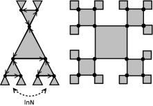
Figure 2. [32] Local structure of some $(\ell,c)$-regular Husimi graphs, with $\ell$ the cycle length and $c$ the cycle connectivity. Left: directed $(3,2)$-regular Husimi graph. Right: undirected $(4,2)$-regular Husimi graph. The Husimi graphs are infinite dimensional as different branches of a central node are separated by a distance of the order $\mathcal{O}(\ln N)$.

3. Spectral analysis of undirected graphs with cycles

In this section we show how to determine the spectral properties of undirected graphs with cycles. For regular graphs, our approach, briefly presented in [32], consists of four steps. First, we write the spectrum in statistical mechanics terms using a complex measure. Then we use the infinite-dimensional nature of the graphs to derive a closed expression in the submatrices of the resolvent. Next, we simplify the resolvent equations to the specific case of regular undirected Husimi graphs. Finally, we solve the resultant algebraic expressions to find analytical expressions for the spectra of regular Husimi graphs.

3.1. Statistical mechanics formulation of the spectrum

We define the resolvent of a real symmetric matrix $A$ as

(3.1) $$\mbox{\boldmath$G$}(z)\equiv\left(z\mbox{\boldmath$I$}_{N}-\mbox{\boldmath$A$}\right)^{-1},$$

where $\mbox{\boldmath$I$}_{N}$ is the $N\times N$ identity matrix and $z\in\mathbb{C}$, with $\rm{Re}(z)=\lambda$ and $\rm{Im}(z)<0$. From the resolvent we can determine the asymptotic density $\rho(\lambda)$ of the real eigenvalues $\lambda$ of an ensemble of symmetric matrices $A$ [4]:

(3.2) $$\rho(\lambda)=\lim_{\rm{Im}(z)\rightarrow 0^{-}}\lim_{N\rightarrow\infty}\frac{1}{\pi N}{\rm Im}\left[{\rm Tr}\mbox{\boldmath$G$}\right].$$

We have left out ensemble averages since we assume that the spectrum self-averages in the limit $N\rightarrow\infty$ to a deterministic value.

A common method in statistical physics is to write the resolvent elements and the spectrum as averages over a certain complex-valued measure $P(\mbox{\boldmath$x$};z)d{\mbox{\boldmath$x$}}$ [11]. Indeed, when defining the normalized Gaussian function

(3.3) $$P(\mbox{\boldmath$x$};z)\sim\exp\left(-\frac{i}{2}\mbox{\boldmath$x$}^{T}\mbox{\boldmath$G$}^{-1}(z)\mbox{\boldmath$x$}\right),$$

the diagonal elements $\left[\mbox{\boldmath$G$}\right]_{ii}=G_{i}$ are given by [36]

(3.4) $$G_{i}=i\langle x^{2}_{i}\rangle,$$

with $\langle\cdot\rangle$ the average with respect to $P(\mbox{\boldmath$x$};z)$. In this formalism the spectrum (3.2) is written as [12]

(3.5) $$\rho(\lambda)=-\lim_{\rm{Im}(z)\rightarrow 0^{-}}\lim_{N\rightarrow\infty}\frac{2}{\pi N}{\rm Im}\left[\frac{\partial}{\partial\lambda}\ln\mathcal{Z}\right]\,,$$

with

(3.6) $$\mathcal{Z}=\int d\mbox{\boldmath$x$}\exp\left(-\frac{i}{2}\mbox{\boldmath$x$}^{T}\mbox{\boldmath$G$}^{-1}(z)\mbox{\boldmath$x$}\right).$$

such that

(3.7) $$\rho(\lambda) = \lim_{\rm{Im}[z]\rightarrow 0^{-}}\frac{1}{\pi N}\sum^{N}_{i=1}{\rm{Im}}G_{i}\left(z\right),\quad{\rm where}\quad\ \lambda=\rm{Re}[z].$$

Hence, in the language of statistical mechanics the spectral density $\rho(\lambda)$ of eigenvalues directly related to the imaginary part of the derivative of the free energy density with respect to $\lambda$, as is seen explicitly in eq.(3.5).

3.2. The resolvent equations

We employ the cavity method to determine the spectral properties of locally tree-like graphs [13, 19]. We construct a matrix $\mbox{\boldmath$A$}^{(i)}$ (and its corresponding resolvent $\mbox{\boldmath$G$}^{(i)}$) through deletion of the $i$-th column and the $i$-th row in $A$. The graph $\mathcal{G}^{(i)}$ induced by the matrix $\mbox{\boldmath$A$}^{(i)}$ is usually referred to as the cavity graph [37]. On this graph we use the Bethe-Peierls tree approximation [37, 38] to arrive at the following set of resolvent equations:

(3.8) $$G^{(j)}_{i}=\frac{1}{z-\sum_{k\in\partial_{i}\setminus j}A^{2}_{ik}G^{(i)}_{k}},\,\,\,\,\,G_{i}=\frac{1}{z-\sum_{k\in\partial_{i}}A^{2}_{ik}G^{(i)}_{k}},$$

where $\partial_{i}$ is the set of vertices neighbouring $i$, and $\partial_{i}\setminus j$ denotes the set of all neighbours of $i$ except for node $j$. In appendix A.1 we report the essential steps in deriving these resolvent equations.

The resolvent equations (3.8) have appeared in the literature for the first time, as far as we know, in the study of electron localization [39]. Similar equations have been derived in the context of Lévy matrices [40] and in the more general context of sparse random graphs [13]. The resolvent equations (3.8) form a set of $2|E|$ equations in $2|E|$-unknowns.

We interpret the set of equations for $\{G_{i}^{(j)}\}$ as a message-passing algorithm along the induced graph $\mathcal{G}$, similar to belief propagation which is widely used in statistical inference and information theory [41]. Here the messages are the diagonal elements of the resolvent of the cavity graph [13].

Next, we extend the resolvent equations (3.8) to Husimi graphs with many short cycles. Although the Bethe-Peierls approximation is no longer valid on these graphs, they still contain an infinite-dimensional character allowing for an analogous approximation. In statistical mechanics this forms the basis for the Kikuchi approximation [42, 43]. For Husimi graphs the Kikuchi approximation gives us the resolvent equations:

(3.9) $$G^{(i)}_{\alpha}=\left(z\mbox{\boldmath$I$}_{\ell-1}-\mbox{\boldmath$D$}^{(i)}_{\alpha}-\mbox{\boldmath$L$}_{\alpha}-\mbox{\boldmath$L$}^{T}_{\alpha}\right)^{-1}\,,$$

with $\alpha\in\partial^{(\ell-1)}_{i}$ and with $\partial^{(\ell-1)}_{i}$ the set of all $(\ell-1)$-tuples $(j_{1},j_{2},\cdots,j_{\ell-1})$ which form a cycle of length $\ell$ with the node $i$. The elements of the $(\ell-1)$-dimensional matrix $\mbox{\boldmath$L$}_{\alpha}$ are $\left[\mbox{\boldmath$L$}_{\alpha}\right]_{nm}=\left[\mbox{\boldmath$L$}_{(j_{1},j_{2},\cdots,j_{\ell-1})}\right]_{nm}=\delta_{n(m+1)}A_{j_{n}j_{m}}$, with $n,m=1,...,(\ell-1)$. The quantity $\mbox{\boldmath$D$}^{(i)}_{\alpha}$ is a diagonal matrix with elements

$$\left[\mbox{\boldmath$D$}^{(i)}_{\alpha}\right]_{kk}=\sum_{\beta\in\partial^{(\ell-1)}_{j_{k}}\setminus(i,j_{1},\ldots,j_{k-1},j_{k+1},\ldots,j_{\ell-1})}\mbox{\boldmath$A$}^{T}_{j_{k},\beta}G^{(j_{k})}_{\beta}\mbox{\boldmath$A$}_{j_{k},\beta}\,,$$

with $\alpha=(j_{1},j_{2},\cdots,j_{\ell-1})$. We have also defined the $(\ell-1)$-dimensional vector $\mbox{\boldmath$A$}^{T}_{j_{k},\beta}=\mbox{\boldmath$A$}_{j_{k},(k_{1},k_{2},\cdots,k_{\ell-1})}=(A_{j_{k}k_{1}}\,\,\,0\,\,\dots\,\,0\,\,\,A_{j_{k}k_{\ell-1}})$. The diagonal elements of the resolvent are given by

(3.10) $$G_{i}=\frac{1}{z-\sum_{\alpha\in\partial^{(\ell-1)}_{i}}\mbox{\boldmath$A$}^{T}_{i,\alpha}G^{(i)}_{\alpha}\mbox{\boldmath$A$}_{i,\alpha}}.$$

In appendix A.2 we elaborate on the precise derivation of these equations.

The resolvent equations (3.9) determine the spectra of graphs with many short cycles of fixed length $\ell$. Note that they can be straightforwardly generalized to graphs with variable cycle lengths and, even more general, to graphs composed from arbitrary figures, by replacing $\mbox{\boldmath$L$}_{\alpha}$ by the corresponding adjacency matrix of the figure $\alpha$ in the absence of a node $i$, and $\mbox{\boldmath$A$}_{j_{k},\beta}$ by the submatrix of $A$ connecting the figure $\beta$ and the node $j_{k}$. In our case, the figures of the graph are the $(\ell-1)$-tuples $\alpha$. The set of resolvent equations (3.9)-(3.10) can also be seen as a message-passing algorithm between regions of the graph, which is similar to the generalized belief propagation algorithm in information theory [43]. Here the messages of the algorithm are the $(\ell-1)\times(\ell-1)$ matrices $\mbox{\boldmath$G$}^{(i)}_{\alpha}$ sent from the $(\ell-1)$-tuples $\alpha$ to a vertex $i$, with whom the tuple $\alpha$ forms a cycle of length $\ell$ in the graph.

We have verified the exactness of the resolvent equations (3.9)-(3.10) on irregular Husimi graphs with $\ell=3$ through a comparison with direct diagonalization results. This is presented in figure 3, where we also compare the spectrum of irregular Husimi graphs with mean cycle connectivity $c=3$ with the spectrum of Erdös-Rényi random graphs with the same mean vertex degree $c=6$. From these results it appears that the spectrum of Erdös-Rényi graphs converges faster to the Wigner semicircle for $c\rightarrow\infty$.

Finally, we point out that the ensemble definitions in section 2 are global by specifying $P(\mbox{\boldmath$A$})$. In the derivation of the resolvent equations (3.9)-(3.10) these global definitions are not explicitely used. Instead, our analysis uses the typical local neighbourhoods of the vertices in the graph. Therefore, our results are valid for all graphs which have a local neighbourhood similar to the one given by the resolvent equations. The connection between the global definitions and the resolvent equations can be made explicit through the distribution of local vertex neighbourhoods, see for instance [19]. This is how we have derived the results in figure 3.

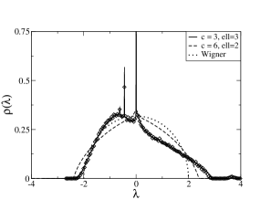
Figure 3. The density of eigenvalues $\lambda$ for an irregular triangular Husimi graph $(\ell=3)$ of mean connectivity $c=3$ with scaling $A_{ij}\rightarrow A_{ij}/\sqrt{2c-1}$ (solid lines) is compared with the eigenvalue density of an irregular Erdös-Rényi graph $(\ell=2)$ of mean connectivity $c=6$ with scaling $A_{ij}\rightarrow A_{ij}/\sqrt{c-1}$ (dashed lines). Both ensembles have the same mean vertex degree. Results from solving the equations (3.9-3.10) for $\ell=3$ with a regulator $\rm{Im}(z)=10^{-4}$ are compared with direct diagonalization results (markers). The dotted line is the Wigner semi-circle law.

In the next two sections we solve the resolvent equations for the case of undirected regular Husimi graphs for which they simplify considerably.

3.3. The resolvent equations for regular undirected graphs

In this section we consider graphs with a simple topology that allows to extract exact analytical solutions from the resolvent equations (3.9)-(3.10): regular Husimi graphs with cycles. For this ensemble of random graphs $\left|\partial^{(\ell-1)}_{i}\right|=c$ and $A_{ij}=1$ for all connected pairs $(i,j)$. In figure 2 the square undirected Husimi graph is illustrated.

Since there is no local disorder every node has the same local neighbourhood. For $N\rightarrow\infty$ the graph becomes transitive and we can set

(3.11) $$G_{\alpha}^{(i)}(z)=\mbox{\boldmath$C$}(z),\qquad G_{i}(z)=G(z)\,,$$

in the resolvent equations (3.9). We get the following closed equations in the $(\ell-1)$-dimensional matrices $C$:

(3.12) $$\mbox{\boldmath$C$}(z)=\left(\begin{array}[]{cccc}z-(c-1)\mathcal{A}^{T}\mbox{\boldmath$C$}(z)\mathcal{A}&-1&0&\cdots\\ -1&z-(c-1)\mathcal{A}^{T}\mbox{\boldmath$C$}(z)\mathcal{A}&-1&\cdots\\ 0&-1&\ddots&\\ \vdots&\vdots&&\ddots\end{array}\right)^{-1},$$

and the resolvent follows from

(3.13) $$G(z)=\frac{1}{z-c\>\mathcal{A}^{T}\mbox{\boldmath$C$}(z)\mathcal{A}\,,}$$

where $\mathcal{A}^{T}=(1\,\,\,0\,\,\dots\,\,0\,\,\,1)$. It is convenient to introduce the scalar variable $G_{s}(z)=\mathcal{A}^{T}\mbox{\boldmath$C$}(z)\mathcal{A}$ and rewrite (3.12) as

(3.14) $$G_{s}(z)=\mathcal{A}^{T}\left(\begin{array}[]{cccc}z-(c-1)G_{s}(z)&-1&0&\cdots\\ -1&z-(c-1)G_{s}(z)&-1&\cdots\\ 0&-1&\ddots&\\ \vdots&\vdots&&\ddots\end{array}\right)^{-1}\mathcal{A}\,.$$

The matrix in (3.14) has a simple structure. We have calculated the inverse analytically using specific methods for tridiagonal matrices [44]. This leads to our final formula for $G_{s}$ when $\ell>2$

(3.15) $$G_{s}=\frac{2n_{\ell-2}+2}{n_{\ell-1}}.$$

The coefficients $n_{2},\dots,n_{\ell-1}$ are complex numbers given by the recurrence relation

(3.16) $$n_{i}=n_{1}n_{i-1}-n_{i-2},\ \ i\geq 2$$

with initial values $n_{0}=1$ and $n_{1}=z-(c-1)G_{s}$. Equations (3.15) and (3.16) are a set of very simple equations that determine the resolvent elements of undirected regular Husimi graphs. It is one of the main results of our previous work [32].

From the expression of $G_{s}$ we find straightforwardly the Green function

(3.17) $$G(z)=\frac{1}{z-c\>G_{s}(z)},$$

and the spectrum, according to eq. (3.7) and (3.17),

(3.18) $$\rho(\lambda)=\frac{c}{\pi}\frac{{\rm Im}G_{s}}{\left(\lambda-c\>{\rm Re}G_{s}\right)^{2}+c^{2}\left({\rm Im}G_{s}\right)^{2}}.$$

3.4. Spectra of regular undirected graphs

We solve the algebraic equations (3.15)-(3.16) to find the spectrum of $(\ell,c)$-regular undirected Husimi graphs. Due to their simple linear structure, these recurrence relations can be solved excactly and allow to obtain the analytical form of the polynomials in the variable $G_{s}$ for any value of $\ell>2$:

• $\ell=3$ corresponds with a quadratic equation:

  $$G_{s}\left[z-(c-1)G_{s}\right]-G_{s}=2.$$

• $\ell=4$ gives a cubic equation:

  $$G_{s}=\frac{2\left[z-(c-1)G_{s}\right]}{\left[z-(c-1)G_{s}\right]^{2}-2}.$$

• $\ell=5$ is determined by a quintic equation:

  $$G_{s}=\frac{2\left[z-(c-1)G_{s}\right]^{3}-4\left[z-(c-1)G_{s}\right]+2}{\left[z-(c-1)G_{s}\right]^{4}-3\left[z-(c-1)G_{s}\right]^{2}+1}.$$

• $\ell=6$ follows from a quartic equation:

  $$G_{s}=\frac{2\left[z-(c-1)G_{s}\right]^{2}-4}{\left[z-(c-1)G_{s}\right]^{3}-3\left[z-(c-1)G_{s}\right]}.$$

• For $\ell>6$, the polynomials have a degree larger than four.

The root of these polynomial equations which gives the expression for the spectrum is a stable fixed point of eq. (3.14). In general, one finds the roots of polynomials in terms of radicals up to degree four. For larger degrees, algebraic solutions in terms of radicals no longer exist, apart from some particular situations [45]. The roots of general polynomials with degree larger than four are given in terms of elliptic functions [45].

We have solved the above equations for $\ell=3,4,6$ and have found the analytical expression for $\rho_{\ell}(\lambda)$, generalizing the Kesten-McKay law [33, 46] to regular graphs with cycles. For other values of $\ell$, eqs. (3.15)-(3.16) are solved numerically in a straightforward way, allowing to study the spectrum as a function of $\ell$ with high accuracy.

From the solution of the resolvent equations, we have found the expressions for the spectra $\rho_{\ell}(\lambda)$ of $(\ell,c)$-regular undirected Husimi graphs. We point out that for $\ell=2$ we recover a sparse regular graph without short cycles. In this case we have the Kesten-Mckay eigenvalue-density distribution [33, 46]

(3.19) $$\rho_{2}(\lambda) = \frac{c}{2\pi}\frac{\sqrt{4(c-1)-\lambda^{2}}}{c^{2}-\lambda^{2}},$$

for $\lambda\in[-2\sqrt{c-1},2\sqrt{c-1}]$, and $\rho_{2}(\lambda)=0$ otherwise. The expression (3.19) follows from solving eq. (3.14).

For $\ell=3$ we recover the spectra $\rho_{3}(\lambda)$ of triangular Husimi graphs [47]

$$\rho_{3}(\lambda) = \frac{2(c-1)}{\pi c}\frac{\sqrt{D_{3}(\lambda)}}{D_{3}(\lambda)+\left[\lambda\frac{2(c-1)}{c}+(1-\lambda)\right]^{2}}+\frac{1}{3}\delta_{c,2}\>\delta(\lambda;-2),$$

for $D_{3}(\lambda)=8(c-1)-(\lambda-1)^{2}>0$, and $\rho_{3}(\lambda)=0$ otherwise. Therefore, the support of $\rho_{3}(\lambda)$ is $\lambda\in[1-2\sqrt{2(c-1)},1+2\sqrt{2(c-1)}]$.

For $\ell=4$ we find the spectrum of a square Husimi graph [32]

$$\rho_{4}(\lambda)=\frac{6\sqrt{3}\,c\,(c-1)\,q_{-}(\lambda)}{\pi\Big{[}2(c-3)\lambda+c\,q_{+}(\lambda)\Big{]}^{2}+3\,\pi\,c^{2}\,q_{-}^{2}(\lambda),}$$

for $D_{4}(\lambda)>0$ and $\rho_{4}(\lambda)=0$ otherwise, where

$$q_{\pm}(\lambda)=s^{1/3}_{+}\pm s^{1/3}_{-},\,\,\,\,\,s_{\pm}(\lambda)=9\lambda(c+1)-\lambda^{3}\pm 9\sqrt{D_{4}(\lambda)},$$

and

$$D_{4}(\lambda)=-\frac{2}{3}\lambda^{4}-\frac{\lambda^{2}}{3}\left(c^{2}-22c+13\right)+\frac{8}{3}(c-2)^{3}.$$

The edges of $\rho_{4}(\lambda)$ are determined by finding the roots of $D_{4}(\lambda)=0$. For $c\rightarrow\infty$, $\rho_{4}(\lambda)$ converges to the Wigner semicircle law. For $c=2$, the spectrum contains a power-law divergence $\rho_{4}(\lambda)\sim|\lambda|^{-1/3}$ as $|\lambda|\rightarrow 0$.

We have also found the analytical expression for $\ell=6$:

$$\rho_{6}(\lambda)=\frac{4c\sqrt{R(\lambda)F(\lambda)}}{\pi R(\lambda)\left[\frac{(c-4)}{(c-1)}|\lambda|+2cR(\lambda)\right]^{2}+\pi c^{2}F(\lambda)},$$

for $D_{6}(\lambda)>0$ and $\rho_{6}(\lambda)=0$ otherwise, with

$$u_{R}(\lambda) = \left(r(\lambda)+\sqrt{D_{6}(\lambda)}\right)^{\frac{1}{3}}+\left(r(\lambda)-\sqrt{D_{6}(\lambda)}\right)^{\frac{1}{3}}+\frac{\left[2c-5+3\lambda^{2}\right]}{3(c-1)^{2}},$$

$$R(\lambda) = \sqrt{u_{R}(\lambda)-\frac{3\lambda^{2}}{4(c-1)^{2}}-\frac{(2c-5)}{(c-1)^{2}}},$$

$$F(\lambda) = -\frac{|\lambda|^{3}}{(c-1)^{3}}+\frac{4(2c+1)|\lambda|}{(c-1)^{3}}+4R(\lambda)\left[\frac{(2c-5)}{(c-1)^{2}}-\frac{3\lambda^{2}}{2(c-1)^{2}}+u_{R}(\lambda)\right],$$

and

$$D_{6}(\lambda) = q^{3}(\lambda)+r^{2}(\lambda),$$

$$q(\lambda)\>(c-1)^{4} = \frac{-9\lambda^{2}+48(c-1)-(2c-5)^{2}}{9},$$

$$r(\lambda)\>(c-1)^{5} = \left[\frac{(4c-7)^{2}-(4c-7)(2c-5)}{2(c-1)}+\frac{(2c-5)^{2}}{3(c-1)}+\frac{(34-16c)}{3}\right]\lambda^{2}$$

$$+\frac{16(2c-5)}{3}+\frac{(2c-5)^{3}}{27(c-1)}.$$

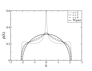
Figure 4. Spectra of $(4,c)$-regular undirected Husimi graphs of connectivity $c=2,3,4$ and with a scaling $A_{ij}\rightarrow A_{ij}/\sqrt{2c-1}$. The spectrum converges to the Wigner semi-circle law for $c\rightarrow\infty$.

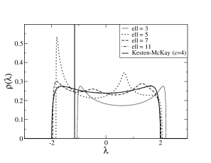
Figure 5. Spectra of $(\ell,2)$ regular undirected Husimi graphs with a scaling $A_{ij}\rightarrow A_{ij}/\sqrt{2c-1}$ and with cycle lengths $\ell=3,5,7,11$. The spectrum converges to the Kesten-McKay law for $\ell\rightarrow\infty$.

The function $D_{6}(\lambda)$ is the discriminant of the cubic polynomial associated to the quartic polynomial for $G_{s}$. The edges of $\rho_{6}(\lambda)$ are obtained from the roots of $D_{6}(\lambda)=0$. The spectrum converges to the Wigner semicircle law when $c\rightarrow\infty$.

For $\ell=5$ and $\ell\geq 7$ we obtain the spectrum by solving numerically the set of eqs. (3.15)-(3.16). One can show that $\rho_{\ell}(\lambda)$ converges to the Wigner law in the limit $c\rightarrow\infty$, and converges to the Kesten-Mckay law in the limit $\ell\rightarrow\infty$ (this limit corresponds to a graph without short cycles).

In figure 4 we present the evolution of the spectrum as a function of the connectivity $c$ for the case $\ell=4$. We notice indeed the fast convergence to the Wigner semi-circle law for $c\rightarrow\infty$. In figure 5 we present the evolution of the spectrum as a function of the cycle length $\ell$, for fixed $c=2$. We see how the spectrum converges rapidly to the Kesten-McKay law for $\ell\rightarrow\infty$.

4. Spectral analysis of directed graphs with cycles

In our study of spectral properties of regular directed graphs with cycles we follow again four steps. First, we write the spectrum in statistical mechanics terms [14]. This is done by mapping the resolvent calculation of a directed graph on a resolvent calculation of a related undirected graph, using the Hermitization procedure [48]. The resolvent of this undirected graph is then analyzed using the methodology presented in section 3. Thereby, the infinite-dimensional nature of the resultant graphs again allows to derive a closed expression in submatrices of the resolvent matrix. Thirdly, we show how this closed set of equations determines the spectrum of directed regular Husimi graphs and we derive their explicit form in this case. Finally, the resultant algebraic expressions are solved to arrive at explicit analytical expressions in the support of the spectra.

4.1. Statistical mechanics formulation of the spectrum

The eigenvalues $\lambda_{1},\dots,\lambda_{N}$ of the $N\times N$ adjacency matrix $A$ of directed Husimi graphs are distributed in the complex plane, contrary to the real eigenvalues for undirected Husimi graphs. By introducing $\partial^{*}=\frac{1}{2}\left(\frac{\partial}{\partial x}+i\frac{\partial}{\partial y}\right)$ and using the relation $\partial^{*}(x+iy)^{-1}=\pi\delta(x)\delta(y)$, the density of states $\rho(\lambda)=N^{-1}\sum_{\mu=1}^{N}\delta(x-{\rm Re}\lambda_{\mu})\delta(y-{\rm Im}\lambda_{\mu})$ at a certain point $\lambda=x+iy$ can be written formally as $\rho(\lambda)=\lim_{N\rightarrow\infty}(N\pi)^{-1}\partial^{*}{\rm Tr}\mbox{\boldmath$G$}(\lambda)$, where $\mbox{\boldmath$G$}(\lambda)$ is the resolvent $\mbox{\boldmath$G$}(\lambda)=(\lambda-\mbox{\boldmath$A$})^{-1}$. The operation $(\cdot)^{*}$ denotes complex conjugation. The $N\times N$ resolvent $\mbox{\boldmath$G$}(\lambda)$ is the central object of interest and its non-analytic behavior at the eigenvalues of $A$ poses difficulties in applying various techniques well-developed for Hermitian matrices [48]. An elegant way to avoid this problem is the Hermitization method. We define a $2N\times 2N$ block matrix

(4.1) $$\mbox{\boldmath$H$}_{\epsilon}(\lambda)=\left(\begin{array}[]{cc}\epsilon\mbox{\boldmath$I$}_{N}\hfill&-i(\lambda-\mbox{\boldmath$A$})\\ -i(\lambda^{*}-\mbox{\boldmath$A$}^{T})&\epsilon\mbox{\boldmath$I$}_{N}\hfill\end{array}\right)\,,$$

where $\epsilon>0$ is a regularizer and $\mbox{\boldmath$I$}_{N}$ is the $N$-dimensional identity matrix. The lower-left block of $\lim_{\epsilon\rightarrow 0^{+}}\mbox{\boldmath$H$}^{-1}_{\epsilon}(\lambda)$ is precisely the matrix $\mbox{\boldmath$G$}(\lambda)$. Thus, the problem reduces to calculating the diagonal matrix elements $\mathcal{G}_{j}(\lambda,\epsilon)=\left[\mbox{\boldmath$H$}^{-1}_{\epsilon}(\lambda)\right]_{j+N,j}$ ($j=1,\dots,N$), from which the spectrum is determined according to

(4.2) $$\rho(\lambda)=-\frac{i}{N\pi}\lim_{\epsilon\rightarrow 0^{+},N\rightarrow\infty}\sum_{j=1}^{N}\partial^{*}\mathcal{G}_{j}(\lambda,\epsilon)\,.$$

The form of the enlarged matrix $H$ depends on the problem at hand and different proposals have appeared in the literature [48, 49, 50, 51]. The form (4.1) is particularly convenient here, since its Hermitian part is a positive-definite matrix and one can represent $\mbox{\boldmath$H$}^{-1}$ as a Gaussian integral. For this purpose we introduce a set of two-dimensional column vectors $\{\mbox{\boldmath$\Phi$}_{i}\}_{i=1,\dots,N}$ with complex elements and the “Hamiltonian” function

(4.3) $$\mathcal{H}(\{\mbox{\boldmath$\Phi$}_{j},\mbox{\boldmath$\Phi$}_{j}^{\dagger}\};\lambda)=\sum_{i=1}^{N}\mbox{\boldmath$\Phi$}_{i}^{\dagger}.\mbox{\boldmath$S$}_{\epsilon}(\lambda)\mbox{\boldmath$\Phi$}_{i}+i\sum_{i,j=1}^{N}\mbox{\boldmath$\Phi$}_{i}^{\dagger}.\mathcal{J}_{ij}\mbox{\boldmath$\Phi$}_{j}\,,$$

where

(4.6) $$\mathcal{J}_{ij}=\left(\begin{array}[]{cc}0&A_{ij}\\ A_{ji}&0\end{array}\right),\,\,$$

and $\mbox{\boldmath$S$}_{\epsilon}(\lambda)=\left[\epsilon\mbox{\boldmath$I$}_{2}-i\left(x\sigma_{x}-y\sigma_{y}\right)\right]$, with ($\sigma_{x},\sigma_{y}$) denoting Pauli matrices.

A graphical representation using an induced graph is again useful in these calculations. For a non-Hermitian matrix with real entries the induced graph is directed, contrary to an undirected graph for real symmetric matrices. Graphically the matrix elements $A_{ij}$ correspond then with a directed edge from node $i$ to node $j$.

Combining the representation of $\left[\mbox{\boldmath$H$}^{-1}_{\epsilon}(\lambda)\right]_{ij}$ as a Gaussian integral with eq. (4.3), $\mathcal{G}_{k}(\lambda,\epsilon)$ reads

(4.7) $$\mathcal{G}_{k}(\lambda,\epsilon) = \frac{1}{2}\int\left[\prod_{j=1}^{N}d\mbox{\boldmath$\Phi$}_{j}d\mbox{\boldmath$\Phi$}^{\dagger}_{j}\right]\left[\mbox{\boldmath$\Phi$}^{\dagger}_{k}.(\sigma_{x}+i\sigma_{y})\mbox{\boldmath$\Phi$}_{k}\right]\mathcal{P}(\{\mbox{\boldmath$\Phi$}_{j},\mbox{\boldmath$\Phi$}^{\dagger}_{j};\lambda\})\,,$$

where we have introduced the complex-valued measure $\prod_{j=1}^{N}\mathcal{P}(\{\mbox{\boldmath$\Phi$}_{j},\mbox{\boldmath$\Phi$}^{\dagger}_{j}\};\lambda)d\mbox{\boldmath$\Phi$}_{j}d\mbox{\boldmath$\Phi$}^{\dagger}_{j}$

(4.8) $$\mathcal{P}(\{\mbox{\boldmath$\Phi$}_{i},\mbox{\boldmath$\Phi$}^{\dagger}_{i}\};\lambda)=\frac{\exp{\left[-\mathcal{H}(\{\mbox{\boldmath$\Phi$}_{i},\mbox{\boldmath$\Phi$}^{\dagger}_{i}\};\lambda)\right]}}{\int\left[\prod_{j=1}^{N}d\mbox{\boldmath$\Phi$}_{j}d\mbox{\boldmath$\Phi$}^{\dagger}_{j}\right]\exp{\left[-\mathcal{H}(\{\mbox{\boldmath$\Phi$}_{i},\mbox{\boldmath$\Phi$}^{\dagger}_{i}\};\lambda)\right]}}\,.$$

Equation (4.7) shows that the local marginals $\{\mathcal{P}(\mbox{\boldmath$\Phi$}_{k},\mbox{\boldmath$\Phi$}^{\dagger}_{k};\lambda)\}_{k=1,\dots,N}$ determine the functions $\{\mathcal{G}_{k}\}_{k=1,\dots,N}$, from which the spectrum follows through eq. (4.2).

4.2. The resolvent equations

We use again the infinite dimensional nature of Husimi graphs to derive an exact equation in the resolvent elements. Due to the sparse structure of $A$, the average number of nodes in a path connecting two randomly chosen cycles scales as $\ln N$ (see figure 8). This fundamental property allows to compute $\{\mathcal{P}(\mbox{\boldmath$\Phi$}_{k},\mbox{\boldmath$\Phi$}^{\dagger}_{k})\}_{k=1,\dots,N}$ using the cavity method, as demonstrated in appendix A.2. The main difference with the undirected case resides in the “state variables” describing the nodes of the graph and the corresponding “Hamiltonian”. While in the undirected case they are scalar real variables, here there is a two-dimensional complex-vector $\mbox{\boldmath$\Phi$}_{i}$ associated to each vertex and they mutually interact through $\mathcal{J}_{ij}$, see eq. (4.3). Hence the resolvent equations involve two-dimensional matrices.

Extending the cavity formulation [14] to directed graphs with cycles, see appendix A.2, we have derived the following equation

(4.9) $$\mathcal{G}_{i}(\lambda,\epsilon)=\left(\mbox{\boldmath$S$}_{\epsilon}(\lambda)+\sum_{\alpha\in\partial^{(\ell-1)}_{i}}\mathbb{A}^{T}_{i\alpha}\mathcal{D}_{\alpha}^{(i)}\mathbb{A}_{i\alpha}\right)^{-1}_{21}\,,$$

where $\partial^{(\ell-1)}_{i}$ is the set of all $(\ell-1)$ tuples $(j_{1},j_{2},\cdots,j_{\ell-1})$ which form a cycle of length $\ell$ with node $i$. The $2\times 2(\ell-1)$ block matrix $\mathbb{A}^{T}_{i\alpha}=(\mathcal{J}_{ij_{1}}\,\,\,\mbox{\boldmath$0$}\,\,\dots\,\,\mbox{\boldmath$0$}\,\,\,\mathcal{J}_{ij_{\ell-1}})$ encodes the interaction between $i$ and a given tuplet $\alpha=(j_{1},j_{2},\cdots,j_{\ell-1})$. The matrix $\mathrm{𝟎}$ is a two-dimensional matrix filled with zeros. The $2(\ell-1)\times 2(\ell-1)$ block matrices $\mathcal{D}_{\alpha}^{(i)}=\mathcal{D}_{(j_{1},j_{2},\cdots,j_{\ell-1})}^{(i)}$ fulfill the cavity equations

(4.10) $$\mathcal{D}_{\alpha}^{(i)}=\left(\mbox{\boldmath$S$}_{\epsilon}(\lambda)\otimes\mbox{\boldmath$I$}_{\ell-1}+\mathcal{B}_{\alpha}^{(i)}+i\mathbb{L}_{\alpha}+i\mathbb{L}_{\alpha}^{T}\right)^{-1},$$

where $i=1,\dots,N$ and $\alpha\in\partial^{(\ell-1)}_{i}$. The matrix $\mathbb{L}_{\alpha}$ is composed of $2\times 2$ block elements defined by $[\mathbb{L}_{\alpha}]_{nm}=[\mathbb{L}_{(j_{1},j_{2},\cdots,j_{\ell-1})}]_{nm}=\delta_{n,m+1}\,\mathcal{J}_{j_{n},j_{m}}$, where $n=2,\dots,\ell-1$. The matrix $\mathcal{B}_{\alpha}^{(i)}$ is a diagonal matrix formed by the following $2\times 2$ block elements

(4.11) $$[\mathcal{B}_{\alpha}^{(i)}]_{kk}=\sum_{\beta\in\partial^{(\ell-1)}_{j_{k}}\setminus(i,j_{1},\ldots,j_{k-1},j_{k+1},\ldots,j_{\ell-1})}\mathbb{A}^{T}_{j_{k}\beta}\mathcal{D}_{\beta}^{(j_{k})}\mathbb{A}_{j_{k}\beta},$$

with $k=1,\dots,\ell-1$ and $\alpha=(j_{1},j_{2},\cdots,j_{\ell-1})$.

Once eqs. (4.10) have been solved, the spectrum follows from eqs. (4.9) and (4.2). The cavity equations have an interpretation in terms of a message-passing algorithm: the matrix $\mathcal{D}_{\alpha}^{(i)}$ is seen as the message sent by the $(\ell-1)$ nodes of cycle $\alpha$ to node $i$ of the same cycle [43]. This completes the general solution of the problem.

4.3. The resolvent equations for regular directed graphs

We determine now the resolvent equations for the spectrum $\rho_{\ell}$ of infinitely large $(\ell,c)$-regular directed Husimi graphs. These graphs have $|\partial^{(\ell-1)}_{i}|=c$ for $i=1,\dots,N$, i.e., each vertex is incident to $c$ cycles of length $\ell$. We set $A_{ij}=1$ and $A_{ji}=0$ when there is a directed edge from node $i$ to $j$, such that the corresponding matrix $\mathcal{J}_{ij}$ assumes the form $\mathcal{J}=\frac{1}{2}(\sigma_{x}+i\sigma_{y})$. As a consequence, the matrices $\{\mathcal{D}_{\beta}^{(i)},\mathbb{A}_{i\beta},\mathbb{L}_{\beta}\}$ become independent of the indices ($i,\beta$). It is convenient to define the two-dimensional matrix $\mbox{\boldmath$G$}_{A}=\mathbb{A}^{T}\mathcal{D}\mathbb{A}$, where $\mathbb{A}^{T}=(\mathcal{J}\,\,\,\mbox{\boldmath$0$}\,\,\dots\,\,\mbox{\boldmath$0$}\,\,\,\mathcal{J}^{T})$. We write $\rho(\lambda)$ in terms of $\mbox{\boldmath$G$}_{A}$ as follows

(4.12) $$\rho_{\ell}(\lambda)=\frac{1}{i\pi}\lim_{\epsilon\rightarrow 0}\partial^{*}\left[\mbox{\boldmath$S$}_{\epsilon}(\lambda)+c\,\mbox{\boldmath$G$}_{A}\right]_{21}^{-1}\,.$$

From eqs. (4.10) and (4.11) one obtains that, for $\ell>2$, the two-dimensional matrix $\mbox{\boldmath$G$}_{A}$ solves the equation

(4.13) $$\mbox{\boldmath$G$}_{A}=\mathbb{A}^{T}\Big{[}\big{(}\mbox{\boldmath$S$}_{\epsilon}(\lambda)+(c-1)\mbox{\boldmath$G$}_{A}\big{)}\otimes\mbox{\boldmath$I$}_{l-1}+i\mathcal{J}\otimes\mbox{\boldmath$L$}_{\ell-1}+i\mathcal{J}^{T}\otimes\mbox{\boldmath$L$}_{\ell-1}^{T}\Big{]}^{-1}\mathbb{A}\,,$$

where $\mbox{\boldmath$L$}_{\ell-1}$ is a $(\ell-1)$-dimensional matrix with elements $[\mbox{\boldmath$L$}_{\ell-1}]_{ij}=\delta_{i,j+1}$. The derivative of eq. (4.13) yields an equation in $\partial^{*}\mbox{\boldmath$G$}_{A}$, which has to be solved together with (4.13) to find $\rho_{\ell}(\lambda)$ through eq. (4.12).

Equation (4.13) allows to derive accurate numerical results for the spectrum of directed Husimi graphs as a function of $\ell$. As an illustration, we present in figure 6 some cuts of $\rho_{3}(\lambda)$ and $\rho_{4}(\lambda)$ along the real direction for fixed values of $y$. These results correspond very well with direct diagonalization, confirming the exactness of (4.13). For a three-dimensional graph of $\rho_{3}(\lambda)$ we refer the reader to [32].

(a) $\ell=3$

(b) $\ell=4$

Figure 6. Three cuts of the spectrum $\rho_{\ell}(\lambda)$ of $(\ell,c)$-regular directed Husimi graphs along the real direction for $c=2$, $\ell=3$ [32] and $c=2$, $\ell=4$. These results (solid lines) are obtained from the numerical solution of eq. (4.13) and they are compared with direct diagonalization results (markers) for an ensemble of $3\times 10^{4}$ matrices of dimension $N=10^{3}$.

Analogously to undirected Husimi graphs, $\rho_{\ell}(\lambda)$ converges to the spectrum of a directed regular graph without short cycles for $\ell\rightarrow\infty$ [20, 31, 52]:

(4.14) $$\rho_{\infty}(\lambda)=\frac{c-1}{\pi}\left(\frac{c}{c^{2}-|\lambda|^{2}}\right)^{2}\,,$$

for $|\lambda|^{2}<c$, and $\rho_{\infty}(\lambda)=0$ otherwise. This convergence is shown numerically in [32]. By rescaling $A_{ij}\rightarrow A_{ij}/\sqrt{c-1}$, the solution of (4.13) leads to Girko’s law in the limit $c\rightarrow\infty$.

4.4. The spectral boundaries for regular directed graphs

In order to derive analytical equations for the support of $\rho_{\ell}(\lambda)$, we determine the inverse of the $2(\ell-1)\times 2(\ell-1)$ matrix present in eq. (4.13). Since this matrix has a tridiagonal block structure its inverse can be computed analytically using the method in [44]. Applying this scheme to the matrix in eq. (4.13), we have simplified (4.13) into an equation involving sums and products of only two-dimensional matrices. This equation forms the equivalent for directed regular graphs of the equation (3.15) for undirected regular graphs. The resultant equations in $\mbox{\boldmath$G$}_{A}$ can be solved using the following ansatz [14]

(4.15) $$\mbox{\boldmath$G$}_{A}=\left(\begin{array}[]{cc}a&ib\\ ib^{*}&d\end{array}\right)\,,$$

where $b$ is complex and $a$ and $d$ are both real variables. The Hermitian part of this matrix is positive-definite provided that $a$ and $d$ are positive. This condition ensures that the Gaussian integrals in the cavity method are convergent [14]. Solving numerically eq. (4.13) for a finite regularizer $\epsilon>0$, we find that $a>0$ and $d>0$. In the limit $\epsilon\rightarrow 0^{+}$, $a$ and $d$ vanish at the boundary of $\rho(\lambda)$. Therefore, setting $\epsilon\rightarrow 0^{+}$ and $a=d=0$ in eq. (4.13), and solving the resulting equations for $b$ leads to an analytical expression for the support of $\rho_{\ell}(\lambda)$. In this way we obtain the following equations for $b$ and $\lambda$ at the boundaries of the support:

• $\ell=3$:

  (4.16) $$b =\frac{\left[\lambda^{*}-(c-1)b^{*}\right]^{2}}{|\lambda-(c-1)b|^{4}},$$

  (4.17) $$|\lambda -(c-1)b|^{4}=(c-1)\left[1+|\lambda-(c-1)b|^{2}\right].$$

• $\ell=4$:

  (4.18) $$b =\frac{\left[\lambda^{*}-(c-1)b^{*}\right]^{2}}{|\lambda-(c-1)b|^{6}},$$

  (4.19) $$|\lambda -(c-1)b|^{6}=(c-1)\left[1+|\lambda-(c-1)b|^{2}+|\lambda-(c-1)b|^{4}\right].$$

The solutions of the polynomials (4.17) and (4.19) in the variable $s\equiv|\lambda-(c-1)b|$ are given by

• $\ell=3$:

  (4.20) $$s=\left[\frac{(c-1)}{2}\left(1+\sqrt{1+\frac{4}{(c-1)}}\right)\right]^{\frac{1}{2}}\,,$$

• $\ell=4$:

  (4.21) $$s=\left[[R_{+}(c)]^{\frac{1}{3}}+[R_{-}(c)]^{\frac{1}{3}}+\frac{1}{3}(c-1)\right]^{\frac{1}{2}}\,,$$

where we have defined

$$R_{\pm}(c) = \frac{1}{27}(c-1)^{3}+\frac{1}{3}(c-1)^{2}\left(\frac{1}{2}\pm F(c)\right)+\frac{1}{2}(c-1)\,,$$

$$F(c) = \left[\frac{1}{81}(c-1)^{2}+\frac{1}{9}(c-1)\kappa+\frac{1}{4}\kappa^{2}-\frac{1}{81}(c-1)^{2}\kappa^{3}\right]^{\frac{1}{2}}\,,$$

with $\kappa=1+\frac{3}{(c-1)}$. By parametrizing $\lambda-(c-1)b=s\exp{(it)}$, with $t\in[0,2\pi]$, and substituting this form in eqs. (4.16) and (4.18), we find the following expressions for the boundary of the support $\lambda_{\ell}(t)$ of triangular $(\ell=3)$ and square $(\ell=4)$ regular directed Husimi graphs:

• $\ell=3$:

  (4.22) $$\lambda_{3}(t)=s\exp{(it)}+\frac{(c-1)}{s^{2}}\exp{(-2it)}\,,$$

• $\ell=4$:

  (4.23) $$\lambda_{4}(t)=s\exp{(it)}+\frac{(c-1)}{s^{3}}\exp{(-3it)}\,.$$

These are the parametric equations which describe, for each corresponding $\ell$, an hypotrochoid in the complex plane. The parameter $s$ as a function of the cycle degree $c$ for $\ell=3$ and $\ell=4$ is given by, respectively, eqs. (4.20) and (4.21).

A hypotrochoid is a cyclic function in the complex plane which is drawn by rotating a small circle of radius $r$ in a larger circle of radius $R$ [53]. The support of triangular and square Husimi graphs is therefore given by hypotrochoids with, respectively, $R/r=3$ and $R/r=4$. These analytical results for the support of the spectra of directed Husimi graphs for $\ell=3$ and $\ell=4$ are shown in the lower graphs of figure 7. The agreement with direct diagonalization results for $c=2$ is excellent, confirming the exactness of our analytical results.

Figure 7. Analytical solutions for the boundary of the support of directed $(\ell,c)$-regular Husimi graphs for several values of the cycle length $\ell$ and the following values $c$ of the number of cycles incident to each vertex: $c=2$ (solid line), $c=3$ (dashed line), $c=4$ (dotted line) and $c=5$ (dot-dashed line). The hypotrochoids have a rotational symmetry by the angle $2\pi/\ell$, from which one obtains the value of the cycle length $\ell$. Direct diagonalization results (dots) for $N\times N$ matrices with $N=1000$ and $c=2$ are shown.

Based on the form of eqs. (4.16-4.19), we conjecture that, for a given $\ell$ and $c$, the following equations are fulfilled at the boundary of the support of $\rho_{\ell}(\lambda)$

(4.24) $$b = \frac{\left[\lambda^{*}-(c-1)b^{*}\right]^{\ell-1}}{s^{2(\ell-1)}}\,,$$

(4.25) $$s^{2(\ell-1)} = (c-1)\sum_{n=0}^{\ell-2}s^{2n}\,.$$

Substituting $\lambda-(c-1)b=s\exp{(it)}$ ($t\in[0,2\pi]$) in eq. (4.24) reads

(4.26) $$\lambda_{\ell}(t)=s\exp{(it)}+\frac{(c-1)}{s^{\ell-1}}\exp{\left[-i(\ell-1)t\right]}\,$$

for the boundary of the support of a $(\ell,c)$ directed regular Husimi graph. Remarkably, eq. (4.26) is a hypotrochoid with a fraction $R/r=\ell$. The parameter $s$ is determined from the roots of a polynomial of degree $\ell$ in the variable $s^{2}$, see eq. (4.25). Equation (4.25) can also be written as

(4.27) $$s^{2}=c-\frac{(c-1)}{s^{2(\ell-1)}}\,.$$

We have found an analytical expression for the roots for $\ell=3$ and $\ell=4$. For larger values of $\ell$, we have solved eq. (4.27) numerically and, by choosing the stable solution, we have derived accurate values for the parameters of the hypotrochoids. We present explicit results for $\ell=5$ and $\ell=6$ in the upper graphs of figure 7. Direct diagonalization results exhibit once more an excellent agreement with the theoretical results, strongly supporting our conjecture that the support of the spectrum of directed regular Husimi graphs for general $\ell$ is given by eqs. (4.26-4.27). The support of regular Husimi graphs converges to the circle $|\lambda|^{2}=c$ in the limit $l\rightarrow\infty$, corresponding with the expression (4.14) for a graph without short cycles.

5. Conclusion

In this work we have obtained the spectra of (un)directed Husimi graphs. The main result is a set of exact equations which determines a belief-propagation like algorithm in the resolvent elements of the matrix. For irregular graphs we have shown a very good correspondence between direct diagonalization results and our approach. For regular graphs we have derived several novel analytical expressions for the spectrum of undirected Husimi graphs and the boundaries of the spectrum of directed Husimi graphs. Remarkably, the boundaries of directed regular Husimi graphs consist of hypotrochoid functions in the complex plane.

Our results indicate that, at high connectivities, the spectrum of undirected random graphs converges to the Wigner semicircle law, while the spectrum of directed random graphs converges to Girko’s circular law. This convergence seems to be rather universal and independent of the specific graph topology. It would be interesting to better understand the conditions under which finitely connected graphs converge to these limiting laws [21, 24, 54, 55].

Finally, we point out that the eigenvalues of random unistochastic matrices are distributed over hypocycloids in the complex plane [56]. This close similarity with our results suggests an interesting connection between the spectra of $\ell\times\ell$ unistochastic matrices and regular directed Husimi graphs with cycles of length $\ell$.

Appendix A Cavity method applied to random matrices

We present the essential steps to determine the resolvent equations using the cavity method [37, 57]. This method is based on the introduction of cavities in a graph $\mathcal{G}$ forming subgraphs $\mathcal{G}^{(i)}$, where the node $i$ and all of its incident edges have been removed, see figure 8. In analogy one can also remove the i-th column and the i-th row from a matrix $A$ to obtain the submatrix $\mbox{\boldmath$A$}^{(i)}$.

A.1. Resolvent equations for locally tree-like graphs

The cavity method is based on the consideration that a probability distribution $P(\mbox{\boldmath$x$};z)$ defined on a locally tree-like graph has the factorization property:

(A.1) $$P^{(j)}_{\partial_{j}}(x_{\partial_{j}};z)=\prod_{k\in\partial_{j}}P^{(j)}_{k}(x_{k};z).$$

The quantity $P^{(j)}_{i}$ is the $i$-th marginal of $P^{(j)}(\mbox{\boldmath$x$};z)$ on the cavity subgraph $\mathcal{G}^{(j)}$ of $\mathcal{G}$, and $P^{(j)}_{\partial_{j}}$ is the marginal of $P^{(j)}(\mbox{\boldmath$x$};z)$ with respect to the set of variables $\partial_{j}$. In the language of spin models, the factorization property follows from the locally tree-like structure of a typical neighbourhood in the graph, see figure 8.

Following the derivation as presented in [13], we find a set of closed equations in the marginals $P^{(j)}_{i}$

$$P^{(j)}_{i}(x_{i};z)\sim\exp\left(-i\frac{zx_{i}^{2}}{2}\right)$$

$$\times\int\left(\prod_{k\in\partial i\setminus j}dx_{k}P^{(i)}_{k}\left(x_{k};z\right)\right)\exp\left(ix_{i}\sum_{k\in\partial_{i}\setminus j}A_{ik}x_{k}\right),$$

from which the marginals $P_{i}$ follow:

$$P_{i}(x_{i};z)\sim\exp\left(-i\frac{zx_{i}^{2}}{2}\right)$$

$$\times\int\left(\prod_{k\in\partial i}dx_{k}P^{(i)}_{k}\left(x_{k};z\right)\right)\exp\left(ix_{i}\sum_{k\in\partial_{i}}A_{ik}x_{k}\right).$$

Finally, we use the fact that the $P^{(j)}_{i}$ are Gaussian functions

(A.4) $$P^{(j)}_{i}(x_{i};z)=\sqrt{\frac{i}{2\pi G^{(j)}_{i}(z)}}\exp\left(-i\frac{x_{i}^{2}}{2G^{(j)}_{i}(z)}\right),$$

to recover the resolvent equations (3.8), after substitution of (A.4) in (LABEL:eq:marg) and (LABEL:eq:marg2).

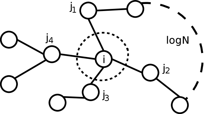
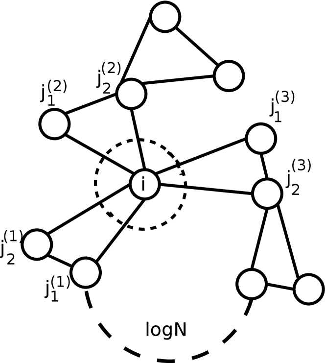
Figure 8. Left: a graph with a locally tree-like structure. Introducing a cavity at the vertex $i$ decouples neighbouring vertices (in the sense that their mutual distance scales with ${\rm log}(N)$). Right: a Husimi graph. After introducing a cavity at the vertex $i$ neighbouring pair of nodes become decouple.

A.2. Resolvent equations for Husimi graphs

We apply now a similar logic to graphs with many cycles which have an infinite-dimensional structure. In this case we use the factorization property

(A.5) $$P^{(i)}_{\partial^{(\ell-1)}_{i}}\left(x_{\partial^{(\ell-1)}_{i}};z\right)=\prod_{\alpha\in\partial^{(\ell-1)}_{i}}P^{(i)}_{\alpha}\left(x_{\alpha};z\right).$$

on the marginals of the distribution $P(\mbox{\boldmath$x$};z)$. The factorization property follows from the fact that the average distance between different branches connected to $i$ is of the order $\ln N$ after removal of $i$, see figure 8. Note that $P^{(i)}_{\alpha}$ is the marginal of $P(\mbox{\boldmath$x$};z)$ for a $(\ell-1)$ tuple $\alpha=(j_{1},\dots,j_{\ell-1})$ forming a cycle with the $i$-th vertex.

We have generalized the derivation for regular Husimi graphs presented in [32] to the case of arbitrary Husimi graphs. We find a set of closed equations in the marginals $P^{(i)}_{\alpha}$:

$$P^{(i)}_{\alpha}\left(x_{\alpha};z\right)\sim\exp\left(-\frac{iz}{2}\sum^{\ell-1}_{k=1}x^{2}_{j^{(\alpha)}_{k}}+i\sum^{\ell-2}_{k=1}A_{j^{(\alpha)}_{k}\>j^{(\alpha)}_{k+1}}\>\>x_{j^{(\alpha)}_{k}}x_{j^{(\alpha)}_{k+1}}\right)$$

$$\times\int\prod_{j\in\alpha}\left[\prod_{\beta\in\partial^{(\ell-1)}_{j}\setminus\alpha}dx_{\beta}P^{(j)}_{\beta}\left(x_{\beta};z\right)\right]$$

$$\times\prod_{j\in\alpha}\left[\prod_{\beta\in\partial^{(\ell-1)}_{j}\setminus\alpha}\exp\left(i\sum_{j\in\alpha}\sum_{\beta\in\partial^{(\ell)}_{j}\setminus\alpha}\left(A_{jj^{(\beta)}_{1}}\>\>x_{j^{(\beta)}_{1}}x_{j}+A_{j^{(\beta)}_{\ell-1}j}\>\>x_{j^{(\beta)}_{\ell-1}}x_{j}\right)\right)\right],$$

with the $(\ell-1)$-tuple $\alpha=\left(j^{(\alpha)}_{1},j^{(\alpha)}_{2},\cdots,j^{(\alpha)}_{\ell-1}\right)$. The marginals $P_{i}$ are given as a function of the marginals $P^{(i)}_{\alpha}$:

$$P_{i}\left(x_{i};z\right)\sim\exp\left(-i\frac{zx_{i}^{2}}{2}\right)$$

$$\times\int\prod_{\alpha\in\partial^{(\ell-1)}_{i}}dx_{\alpha}P^{(i)}_{\alpha}\left(x_{\alpha};z\right)\prod_{\alpha}\exp\left(i\>A_{ij^{(\alpha)}_{1}}\>\>x_{j^{(\alpha)}_{1}}\,x_{i}+i\>A_{j^{(\alpha)}_{\ell-1}i}\>\>x_{j^{(\alpha)}_{\ell-1}}\,x_{i}\right).$$

We now use the Gaussian ansatz for the marginals $P^{(i)}_{\alpha}\left(x_{\alpha};z\right)$:

(A.8) $$P^{(i)}_{\alpha}\left(x_{\alpha};z\right)\sim\exp\left(-\frac{i}{2}\mbox{\boldmath$x$}^{T}\left(\mbox{\boldmath$G$}^{(i)}_{\alpha}\right)^{-1}\mbox{\boldmath$x$}\right),$$

with $\mbox{\boldmath$G$}^{(i)}_{\alpha}$ the $(\ell-1)\times(\ell-1)$ submatrix of the resolvent $\mbox{\boldmath$G$}^{(i)}$ of the cavity matrix $\mbox{\boldmath$A$}^{(i)}$:

(A.13) $$\mbox{\boldmath$G$}^{(i)}_{\alpha}=\left(\begin{array}[]{cccc}G^{(i)}_{j^{(\alpha)}_{1}j^{(\alpha)}_{1}}&G^{(i)}_{j^{(\alpha)}_{1}j^{(\alpha)}_{2}}&\cdots&G^{(i)}_{j^{(\alpha)}_{1}j^{(\alpha)}_{\ell-1}}\\ G^{(i)}_{j^{(\alpha)}_{2}j^{(\alpha)}_{1}}&G^{(i)}_{j^{(\alpha)}_{2}j^{(\alpha)}_{2}}&\cdots&G^{(i)}_{j^{(\alpha)}_{2}j^{(\alpha)}_{\ell-1}}\\ \vdots&\vdots&\cdots&\vdots\\ G^{(i)}_{j^{(\alpha)}_{\ell-1}j^{(\alpha)}_{1}}&G^{(i)}_{j^{(\alpha)}_{\ell-1}j^{(\alpha)}_{2}}&\cdots&G^{(i)}_{j^{(\alpha)}_{\ell-1}j^{(\alpha)}_{\ell-1}}\end{array}\right).$$

We also use a Gaussian ansatz of the type (A.4) for the marginal $P_{i}$. Substitution of these ansätze in (LABEL:eq:marginalst) and (LABEL:eq:marginalsTT) gives the resolvent equations (3.9) and (3.10).

We remark that the resolvent equations can also be derived using methods from random matrix theory , i.e. by recursively applying the Schur-complement formula [19, 31].

References

- [1] B. Mohar, Some applications of Laplace eigenvalues of graphs, Graph Symmetry: Algebraic Methods and Applications, Vol. 497 Kluwer (1997), 227-275.
- [2] F. R. K. Chung, Spectral Graph Theory, American Mathematical Society (1997)
- [3] A. E. Brouwer, W. H. Haemers, Spectra of Graphs, Springer (2010).
- [4] B. Mohar, W. Woess, A survey on spectra of infinite graphs, Bull. London Math. Soc. 21 (1989), 209-234.
- [5] A. Barrat, M. Barthélemy, A. Vespignani, Dynamical processes on networks, Cambridge University Press (2008)
- [6] M. E. J. Newman, Networks, An Introduction, Oxford University Press (2010).
- [7] M. Baharona, L. M. Pecora, Synchronization in small-world systems, Phys. Rev. Lett. 89 (2002), 054101.
- [8] S. F. Edwards, D. R. Wilkinson, The surface statistics of granular aggregate, Proc. R. Soc. London, Ser. A 381, 17 (1982); B. Kozma, M. B. Hastings, G. Korniss, Roughness scaling for Edwards-Anderson relaxation in small-world networks, Phys. Rev. Lett. 92, 108701 (2004).
- [9] D. J. Klein, R. Randić, Resistance distance, J. Math. Chem. 12 (1993), 81-95.
- [10] S. Hoory, N. Linial, A. Wigderson, Expander graphs and their applications, Bull. Amer. Math. Soc. 43 (2006), 439-561
- [11] S. F. Edwards, R. C. Jones, The Eigenvalue Spectrum of a Large Symmetric Random Matrix, J. Phys. A 9 (1976), 1595-1603.
- [12] R. Kühn, Spectra of sparse random matrices, J. Phys. A: Math. Theor. 41 (2008), 295002.
- [13] T. Rogers, K. Takeda, I. P. Castillo and R. Kühn, Cavity approach to the spectral density of sparse symmetric random matrices, Phys. Rev. E. 78 (2008), 031116.
- [14] T. Rogers, I. P. Castillo, Cavity approach to the spectral density of non-hermitian sparse matrices, Phys. Rev. E 79 (2009), 012101.
- [15] Y. V. Fyodorov, A. D. Mirlin, On the Density of States of Sparse Random Matrices, J. Phys. A 24 (1991), 2219-2223.
- [16] T. Rogers, C. P. Vicente, K. Takeda, I. P. Castillo, Spectral density of random graphs with topological constraints, J. Phys. A: Math. Theor. 43 (2010), 195002.
- [17] R. Kühn, J. M. van Mourik, Spectra of modular and small-world matrices, J. Phys. A: Math. Theor., 44 (2011), 165205
- [18] Y. Kabashima, H. Takahashi, O. Watanabe, Cavity approach to the first eigenvalue problem in a family of symmetric random sparse matrices, J.Phys.: Conf. Ser. 233 (2010), 012001; Y. Kabashima, H. Takahashi, First eigenvalue/eigenvector in sparse random symmetric matrices: influences of degree fluctuation, J. Phys. A: Math. Theor. 45 (2012), 325001
- [19] C. Bordenave, M. Lelarge, Resolvent of large random graphs , Random Structures and Algorithms 37 (2010), 332.
- [20] C. Bordernave, D. Chafai, Around the circular law, Probability Surveys, 9 (2012), 1-89.
- [21] T. Tao, V. Vu., Random matrices: the circular law, Commun. Contemp. Math.,10, 261-307 (2008).
- [22] T. Tao, V. Vu, M. Krishnapur, Universality of ESDs and the circular law, Ann. Probab. 38, 2023- 2065 (2010).
- [23] F. Götze, A. Tikhomirov, The circular law for random matrices, Ann. Probab., 38, 1444- 1491 (2010).
- [24] P. M. Wood, Universality and the circular law for sparse random matrices, Ann. Appl. Probab. 22, 1266 (2012).
- [25] C. Bordenave, P. Caputo, D. Chafai, Spectrum of Markov generators on sparse random graphs, arXiv:1202.0644 (2012).
- [26] P. M. Gleiss, P. F. Stadler, A. Wagner, D. A. Fell, Small cycles in small worlds, arxiv:cond-mat/0009124 (2000).
- [27] G. Bianconi, G. Caldarelli, A. Capocci, Loops structure of the internet at the autonomous system level, Phys. Rev. E 71 (2005), 066116.
- [28] G. Bianconi, N. Gulbahce, A. E. Motter, Local structure of directed networks, Phys. Rev. Lett. 100 (2008), 118701.
- [29] K. Husimi, Note on Mayers’ theory of cluster integrals, J. Chem. Phys. 18 (1950), 682-684.
- [30] F. Harary, G. Uhlenbeck, On the number of Husimi trees I, Proc. Natl. Acad. Sci. U.S.A. 39 (1953), 315-322.
- [31] I. Neri, F. L. Metz, Spectra of sparse non-Hermitian random matrices: an analytical solution, Phys. Rev. Lett. 109 (2012), 030602
- [32] F. L. Metz, I. Neri, D. Bollé, Spectra of sparse regular graphs with loops, Phys. Rev. E 84 (2011), 055101(R).
- [33] B. D. McKay, The expected eigenvalue distribution of a large regular graph, Linear Algebra Appl. 40 (1981), 203-216.
- [34] O. Khorunzhy, M. Shcherbina, V. Vengerovsky, Eigenvalue distribution of large weighted random graphs, J. Math. Phys. 45 (2004), 1648-1672.
- [35] B. Bollobás, Random Graphs, Cambridge University Press (2001).
- [36] F. L. Metz, I. Neri, D. Bollé, Localization transition in symmetric random matrices, Phys. Rev. E 82 (2010), 03115.
- [37] M. Mézard, A. Montanari, Information, Physics and Computation, Oxford University Press (2009).
- [38] H. A. Bethe, Statistical theory of superlattices, Proc. Roy. Soc. London Ser A 150 (1935), 552-575.
- [39] R. Abou-Chacra, D. J. Thouless, P. W. Anderson, A selfconsistent theory of localization, J. Phys. C: Solid State Phys. 6 (1973), 1734
- [40] P. Cizeau, J. P. Bouchaud,Theory of Lévy matrices, Phys. Rev. E 50 (1994), 1810-1822.
- [41] P. Judea, Probabilistic Reasoning in Intelligent Systems: Networks of Plausible Inference, Morgan Kaufmann (1988), San Francisco, CA.
- [42] R. Kikuchi, A Theory of cooperative phenomena, Phys. Rev. 81 (1951), 988-1003
- [43] W. T. Yedidia, J. S. Freeman, Y. Weiss, Bethe free energy, kikuchi approximations, and belief propagation algorithms, Technical Report TR-2001-16, Mitsubishi Electric Reseach, 2001.
- [44] Y. Huang, W. F. McColl, Analytic inversion of general tridiagonal matrices, J. Phys. A: Math. Gen. 30 (1997), 7917.
- [45] R. B. King, Beyond the quartic equation, Birkhäuser Boston, 1996.
- [46] H. Kesten, Symmetric random walks on groups, Trans. Amer. Math. Soc. 92, (1959) 336354.
- [47] M. Eckstein, M. Kollar, K. Byczuk, D. Vollhardt, Hopping on the Bethe lattice: Exact results for density of states and dynamical mean-field theory, Phys. Rev. B 71, 235119 (2005); M. Galiceanu, A. Blumen, Spectra of Husimi cacti: exact results and applications, J. Chem. Phys.127, 134904 (2007).
- [48] J. Feinberg, A. Zee, Non-hermitian random matrix theory: Method of hermitian reduction, Nucl. Phys. B 504, 579 (1997).
- [49] J. T. Chalker, Z. J. Wang, Diffusion in a random velocity field: Spectral properties of a non-hermitian Fokker-Planck operator, Phys. Rev. Lett. 79, 1797 (1997).
- [50] J. T. Chalker, B. Mehlig, Eigenvector statistics in non-hermitian random matrix ensembles, Phys. Rev. Lett. 81, 3367 (1998).
- [51] R. A. Janik, W. Nörenberg, M. A. Nowak, G.Papp, I. Zahed, Correlation of eigenvectors for non-hermitian random matrix models, Phys. Rev. E 60, 2699 (1999).
- [52] T.Rogers, New results on the spectral density of random matrices, thesis (2010).
- [53] J. D. Lawrence, A Catalog of Special Plane Curves, New York: Dover, pp. 165-168, (1972).
- [54] I. Dumitriu, S. Pal, Sparse regular random graphs: spectral density and eigenvectors , arXiv:0910.5306.
- [55] L. Tran, V. Vu, K. Wang, Sparse random graphs: Eigenvalues and Eigenvectors, arXiv:1011.6646
- [56] K. Życzkowski, M. Kus, W. Słomczynski and H. -J. Sommers, Random unistochastic matrices, J. Phys A: Math. Gen. 36, 3425 (2003).
- [57] M. Mézard, G. Parisi, M.Virasoro, Spin Glass Theory and beyond, World Scientific (1986).