The PTF Orion Project: a Possible Planet Transiting a T-Tauri Star

Abstract

We report observations of a possible young transiting planet orbiting a previously known weak-lined T-Tauri star in the 7–$10\,{\rm Myr}$-old Orion-OB1a/25-Ori region. The candidate was found as part of the Palomar Transient Factory (PTF) Orion project. It has a photometric transit period of $0.448413\pm 0.000040$ days, and appears in both 2009 and 2010 PTF data. Follow-up low-precision radial velocity observations and adaptive-optics imaging suggest that the star is not an eclipsing binary, and that it is unlikely that a background source is blended with the target and mimicking the observed transit. Radial-velocity observations with the Hobby-Eberly and Keck telescopes yield a radial velocity that has the same period as the photometric event, but is offset in phase from the transit center by $\approx-0.22$ periods. The amplitude (half range) of the radial velocity variations is $2.4\,{\rm km}\,{\rm s}^{-1}$ and is comparable with the expected radial velocity amplitude that stellar spots could induce. The radial velocity curve is likely dominated by stellar spot modulation and provides an upper limit to the projected companion mass of $M_{\mathrm{p}}\sin i_{\mathrm{orb}}\lesssim 4.8\pm 1.2\,M_{\rm Jup}$; when combined with the orbital inclination, $i_{\mathrm{orb}}$, of the candidate planet from modeling of the transit lightcurve, we find an upper limit on the mass of the planetary candidate of $M_{\mathrm{p}}\lesssim 5.5\pm 1.4\,M_{\rm Jup}$. This limit implies that the planet is orbiting close to, if not inside, its Roche limiting orbital radius, so that it may be undergoing active mass loss and evaporating.

1 Introduction

The Palomar Transient Factory (PTF) Orion project is a study within the broader PTF survey aimed at searching for photometric variability in the young Orion region, with the primary goal of finding young extrasolar planets (van Eyken et al. 2011). The project is based on a set of intensive high-cadence ($\approx 70$–$90\,\mathrm{s}$) observations of a single $7.26\,\mathrm{deg}^{2}$ field centered on the known 25 Ori (catalog ) association, which lies in the Orion OB1a region and has an estimated age of 7–10$\,{\rm Myr}$ (Briceño et al. 2005, 2007).

Typical young circumstellar disk lifetimes are on the order of 5–$10\,{\rm Myr}$ (Hillenbrand 2008), and it is during this time that the bulk of the formation and migration of planets is expected to occur. The youngest exoplanets have been found via direct detection (Kraus & Ireland 2012, e.g., LkCa 15,; Marsh et al. 2010, the free-floating planetary-mass object in the $\rho$ Oph cloud,); however, little is known empirically about exoplanets during the first few millions of years of their lives, and the goal is to fill the observational gap and begin to provide constraints on theories of planet formation and evolution (see, e.g., Armitage 2009). The stars in the 25 Ori/OB1a region should be at or just beyond the point of disk dissipation, consistent with the high ratio of weak-lined to classical T-Tauri stars found there (Briceño et al. 2007). We can therefore look for planet transits at the time when they may first become observable without their signatures being swamped by the extreme variability characteristic of the younger classical T-Tauri stars. In so doing, we can begin to investigate the frequency of planets at these ages; the timescales for their evolution; the timescales of their migration with respect to the star’s evolution; and, through measurements of the transit depths, probe empirically their mean densities and the extent of their atmospheres, which are expected to be inflated at these early stages (Fortney & Nettelmann 2010, and references therein).

Several surveys have been undertaken to search for close-in young exoplanets, though many are radial-velocity searches (e.g., Esposito et al. 2006; Paulson & Yelda 2006; Setiawan et al. 2007, 2008; Huerta et al. 2008; Crockett et al. 2011; Nguyen et al. 2012). A transit search (e.g., Aigrain et al. 2007; Miller et al. 2008; Neuhäuser et al. 2011) has the advantage of being able to search many more stars simultaneously, down to fainter magnitudes and with a faster cadence. Combining transit photometry with spectroscopic information can provide a wealth of information that is unavailable with non-transiting planets, from masses and radii to constraints on atmospheric composition.

An outline of the PTF Orion project is given by van Eyken et al. (2011), along with some of the first results concerning binary stars and T-Tauri stars. The broader PTF survey is described in detail by Law et al. (2009) and Rau et al. (2009), with a summary of the first year’s performance by Law et al. (2010). Here we report a young planet candidate found orbiting a known M3 pre-main-sequence (PMS) weak-lined T-Tauri star (TTS) within the PTF Orion field. Our observations are outlined in Section 2; Section 3 discusses the photometric and spectroscopic results and some implications. The main conclusions are summarized in section 4.

2 Observations

2.1 PTF Photometry

PTF Orion data were obtained using the Palomar $48\arcsec$ Samuel Oschin telescope during the majority of the clear nights between 2009 December 1 and 2010 January 15, whenever the field was above an airmass of 2.0. All observations were in the $R$ band, and of the 40 nights dedicated, 14 yielded usable data, the remainder being lost primarily to poor weather. Light curves were obtained for $\sim 110,000$ sources within the field, the top $\sim 500$ most variable of which were inspected visually. The observations and the PTF Orion differential photometry pipeline and data reduction details are described fully in van Eyken et al. (2011). Specifics of the more general PTF data reduction pipeline are described by R. Laher et al. (2012, in preparation) and Ofek et al. (2012). Among the inspected sources, one, PTFO 8-8695 (catalog ) (2MASS J05250755+0134243 (catalog )), showed periodic shallow transit-like events with a shape and depth suggestive of a planetary companion, superposed on a larger-scale quasi-periodic variable light curve. The source has previously been identified as a weak-line T-Tauri star (WTTS) associated with the Orion OB1a region by Briceño et al. (CVSO 30 (catalog ), 2005), and Hernández et al. (2007). A summary of the main previously determined properties of the primary star is given in Table 1. In Figure 1 we show a color-magnitude diagram indicating PTFO 8-8695 in relation to the other T-Tauri stars in the OB1a region discovered by Briceño et al. (2005). Although classified as a WTTS, it lies at the younger end of the distribution. This is consistent with its its relatively strong $\mathrm{H}_{\alpha}$ emission, which in fact places it on the borderline with classical T-Tauri stars (CTTS) according to the classification scheme of Briceño et al. (2005).

Table 1: PTFO 8-8695 Stellar Properties

Property	Value
Alternative designations	CVSO 30 (catalog )
	2MASS J05250755+0134243 (catalog )
	PTF1 J052507.55+013424.3 (catalog )
$\alpha$ (J2000)	05$\fh$25$\fm$07$\fs$55
$\delta$ (J2000)	+01$\fdg$34$\farcm$24.3$\farcs$
$V$	16.26 mag
2MASS $J$	$12.232\pm 0.028\,{\rm mag}$
2MASS $H$	$11.559\pm 0.026\,{\rm mag}$
2MASS $K_{S}$	$11.357\pm 0.021\,{\rm mag}$
Median $R$	$15.19\,{\rm mag}$
$R$ range	$0.17\,{\rm mag}$ (min to max)
$\mathrm{H_{\alpha}}$ equiv. width	-11.40Å
LiI equiv. width	0.40 Å
Sp. Type	M3 (PMS weak-lined T-Tauri)
$T_{\mathrm{eff}}$	$3470\,{\rm K}\tablenotemark{a}$
$A_{V}$	$0.12\,{\rm mag}$
Luminosity	$0.25\,{L_{\odot}}$
Radius	$1.39\,{R_{\odot}}$
Mass (Baraffe/Siess)	$0.44\,M_{\odot}/0.34\,M_{\odot}$
Age (Baraffe/Siess)	$2.63\,{\rm Myr}/2.68\,{\rm Myr}$
Distance	$\sim 330\,{\rm pc}$ (mean dist. to OB1a/25 Ori assoc.)

Figure 1: Color-magnitude diagram following Briceño et al. (Figure 7, 2005), highlighting PTFO 8-8695 (CVSO 30) – the star symbol – in relation to the other T-Tauri stars discovered therein (see section 2.1). PTFO 8-8695 lies at the younger end of the distribution. Open circles indicate WTTS; filled circles indicate CTTS. Solid lines indicate, from the top, 1, 3, 10, and $30\,{\rm Myr}$ isochrones, and the zero-age main sequence, according to the models of Siess et al. (2000) at a distance of $330\,{\rm pc}$. Photometric measurements are reproduced from Briceño et al. (2005). Reddening and extinction are neglected.

The same field was again observed in the same way over seven clear nights between 2010 December 8–17. The transit events were again evident with the same period and depth. Owing to improvements in the PTF image processing software, better weather, and mitigation of the CCD fogging effect seen in the previous year’s data (see van Eyken et al. 2011; Ofek et al. 2012), the RMS noise floor for the brightest stars in the 2010 December data set improved from $\approx 4$ to $\approx 3\,{\rm mmag}$, with less evidence of systematic effects. Figures 2 and 3 show the light curves obtained in the first and second years of observations with PTF. The quasi-periodic stellar variability is evident, along with sporadic low-level flaring, consistent with the star’s young age and late spectral type. Visual inspection of the curves revealed the additional regular periodic transit-like signature, with a depth of $\approx 3$–4%, superposed on the stellar variability. We initially determined an approximate period ($\approx 0.45$ days) and transit duration ($\approx 2$ hours) by hand, in order to locate all the transit windows. A detailed discussion of the light curves and derived properties is given in Section 3.1. The regularity and planet-like characteristics of the transit events led us to obtain follow-up observations.

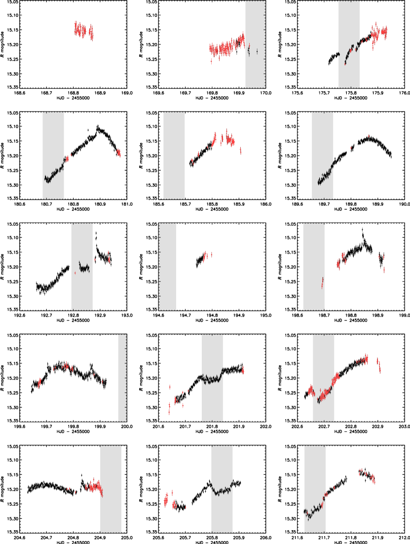
Figure 2: Photometric light curve for 2009 December 1–2010 January 15 (Sections 2.1 and 3.1.1). Gray regions indicate the transit windows, fixed at the measured transit period, width, and epoch of center-transit ($T_{0}$). Red points indicate data automatically flagged by the data reduction software as potentially non-optimal for various possible reasons (e.g., imperfect weather, evidence of contamination within the photometric aperture, etc.)

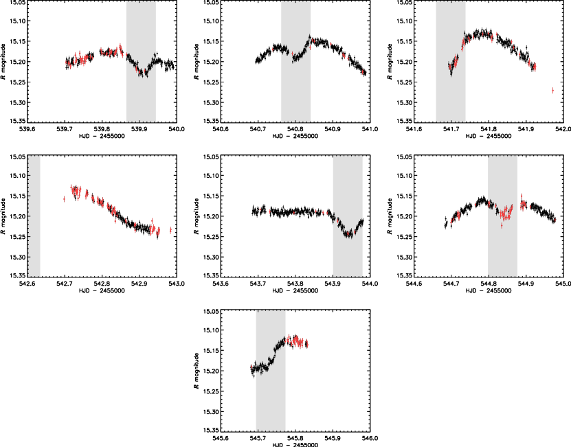
Figure 3: As for Figure 2, for 2010 December 8–17.

2.2 Keck Adaptive Optic Imaging

The PTF imaging instrument is seeing limited and has a point-spread function (PSF) with typical full-width-half-maximum (FWHM) of $2.0\arcsec$, or $660\,{\rm AU}$ at the estimated distance of the Orion OB1a and 25 Ori associations ($330\,{\rm pc}$, Briceño et al. 2005, 2007). We obtained adaptive optics (AO) images using the NIRC2 camera (PI K. Matthews) on the $10\,{\rm m}$ Keck II telescope in order to probe regions in the immediate vicinity of the star and to search for any sources (false positives) that could mimic the signal of a transiting planet, such as a nearby eclipsing binary. At $R=15.2\,{\rm mag}$, PTFO 8-8695 is sufficiently bright for natural guide star observations and does not require the use of a laser for atmospheric compensation. We locked the AO system control loops onto the target using a frame rate of 41 Hz. The airmass was 1.29. We used the NIRC2 narrow camera setting to provide fine spatial sampling ($10\,{\rm mas}\,{\rm pix}^{-1}$). Our observations consisted of 12 dithered H-band images (3 coadds per frame, $10\,\mathrm{s}$ per coadd), totaling 6 minutes of on-source integration time. Raw frames were processed by cleaning hot pixels, subtracting background noise from the sky and detector, and aligning and coadding the results.

Figure 4 shows the final reduced image using an effective field-of-view of $4.9\arcsec\times 4.9\arcsec$, which corresponds to $\approx 4.9$ PTF pixels on a side. The image shows no contaminants, except for one faint source to the south east, at a separation of $1.8\arcsec$ ($590\,{\rm AU}$ in the plane of the sky at the distance of Orion OB1a/25 Ori). Our diffraction-limited images (FWHM $\approx 80\,{\rm mas}$) rule out additional off-axis sources down to a level of $\Delta H=4.3$, 6.4, 8.9, and $9.1\,{\rm mag}$ ($3\sigma$) at angular separations of 0.25″, 0.5″, 1.0″, and $2.0\arcsec$ (83, 165, 330, and 660 pc) respectively. Assuming a color difference of $0\,{\rm mag}$, a faint, blended, 100% eclipsing binary would have to be within $\Delta H\approx 3.5$–$3.8\,{\rm mag}$ of the primary star, or brighter, to mimic the observed transit depth at $R$ of $\approx 3$–4%. At $6.96\,{\rm mag}$ (608 times) fainter than our target, the one imaged contaminant is too faint to be a blended eclipsing binary capable of mimicking the observed transits unless it is extremely blue ($R-H\lesssim-3.2$); in that event, however, it would be unlikely to be stellar in origin in any case. Any other such binary would have to lie within $0.25\arcsec$ of our target in order not to have been detected.

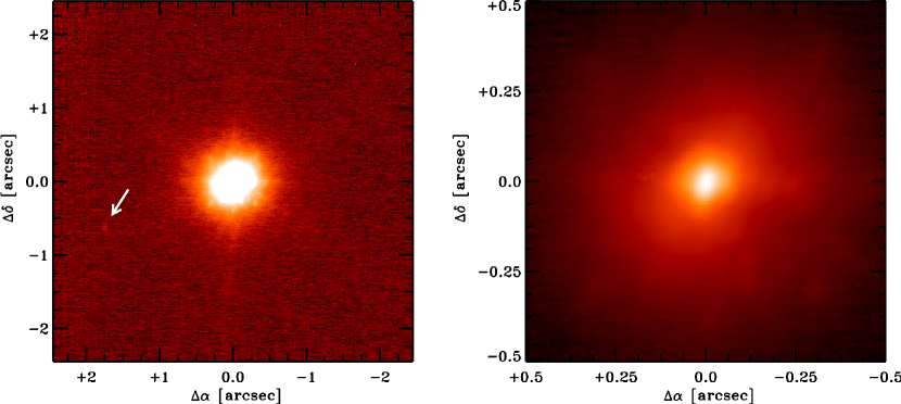
Figure 4: Adaptive optics imaging of PTFO 8-8695, showing the full image field (left), and detail around the central star (right), at two different logarithmic brightness stretches. A very faint source is detected to the south east of the central star at a separation of 1.8″, $6.96\,{\rm mag}$ fainter than the central source, and unlikely to be capable of mimicking the observed transits (indicated by the arrow, left panel); otherwise no contaminants are detected. (Section 2.2.)

2.3 LCOGT, KPNO 4 m, and Palomar 200″ Vetting

Photometric observations were obtained in 2011 February with the Las Cumbres Observatory Global Telescope Network (LCOGT), using the $2\,{\rm m}$ Faulkes North and South telescopes, and the $0.8\,{\rm m}$ Byrne Observatory telescope at Sedgwick Reserve (BOS). We were able to confirm complete transit detections on two separate nights with the BOS telescope with a clear filter (see Figure 5). Observations in SDSS $g^{\prime}$ and $i^{\prime}$ with the three telescopes were inconclusive, and largely hampered by poor observing conditions and sparse phase coverage. The LCOGT observations enabled us to confirm the transit event and its period independently of the PTF data, and, in combination with the PTF data, we were able to establish a more accurate and up-to-date transit ephemeris.

In addition we obtained low-precision followup radial velocity (RV) observations with the KPNO 4 m Mayall telescope and the Palomar $200\arcsec$ Hale telescope over 3 and 2 consecutive nights, respectively, to allow us to rule out a stellar-mass companion as the cause of the transits. The separate confirmation of the transit event and the lack of RV signature at the level of $\sim 10\,{\rm km}\,{\rm s}^{-1}$ suggested that we had indeed detected a sub-stellar object, and we pursued additional observations.

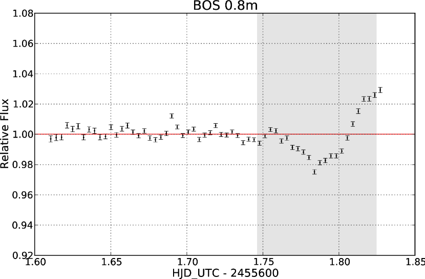
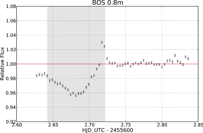
Figure 5: Transit observations obtained with the LCOGT BOS 0.8 m telescope (clear filter), on the nights of 2011 February 8 and 9 (Section 2.3). Gray regions again indicate the predicted transit windows using the period and $T_{0}$ obtained with the PTF data. The second night shows a possible small flare at the end of the transit. Note that in addition to stellar variability, some of the systematic trends may also be air-mass related.

2.4 HET and Keck Spectroscopy

Following the AO vetting and low-precision RV followup, we obtained Doppler radial velocity spectroscopy with both the High Resolution Spectrograph (HRS; Tull 1998) on the $9.2\,{\rm m}$ Hobby Eberly Telescope (HET; Ramsey et al. 1998), and the High Resolution Echelle Spectrometer (HIRES; Vogt et al. 1994) on the $10\,{\rm m}$ Keck I telescope. The goal was to detect or place an upper limit on any signal due to reflex stellar motion caused by the orbiting companion.

The queue-schedule operation mode of the HET (Shetrone et al. 2007) allowed us to obtain four spectroscopic radial velocity observations very quickly after analysis of the low-precision RV and LCOGT photometric vetting data. The observations were timed on the basis of prior knowledge of the transit ephemeris to best constrain any orbital signature.

Observations from the fiber-fed HRS spectrograph and calibrated using ThAr exposures provide radial velocity precision of better than $50\,{\rm m\,s^{-1}}$ over timescales of several weeks (Bender et al. 2012). Seeing-induced PSF changes are minimal due to the image scrambling properties of optical fibers (Heacox 1987) and the HRS temperature is kept stable to $\sim 0.01\,\mathrm{C}$. We used the 15k resolution mode of HRS, with the red cross-disperser setting (316g7940), giving a wavelength coverage of $6114$–$9861\,\text{\AA}$. The use of this lower resolution setting enhances the efficiency of HRS without significantly degrading the information content in the stellar spectrum (since the target absorption lines were already known to be rotationally broadened). Each observation was $1200\,\mathrm{s}$ in duration, except on UT 2011-02-21 which was $1600\,\mathrm{s}$, and ThAr calibration frames were taken immediately after each to track instrument drift. Data for the four nights were reduced in IDL with a custom optimal extraction pipeline that performs bias subtraction, flat fielding, order tracing and extraction, and wavelength calibration of the extracted one-dimensional spectra. A simultaneous sky-fiber was available with this spectrograph setting, but we chose to avoid the additional complexity inherent in performing sky subtraction with a fiber-fed spectrograph, and instead masked areas affected by sky lines so that they were not used in calculating the RVs. The achieved signal to noise in each spectrum was approximately 40–50 per resolution element, peaking in the I-band. We identified the strongest absorption lines in an M2-type high resolution Kurucz stellar model (Kurucz 2005), and used these to select lines for fitting in the measured spectra.

For the Keck data, we observed PTFO 8-8695 using the standard procedures (e.g., Howard et al. 2009) of the California Planet Search (CPS) for HIRES. The five observations over 10 days were each 500–$600\,\mathrm{s}$ in duration and achieved a signal to noise ratio of 10–20 per pixel (S/N = 20–40 per resolution element) in the V-band. We used the “C2” decker ($0.86\arcsec$ wide slit) for a spectral resolution of $\sim$60,000. The total wavelength coverage was $\approx 3650$–$7970\,\text{\AA}$.

Owing to the faintness of the target and the relatively relaxed precision requirements, we employed in both cases thorium-argon (ThAr) emission lamps as the fiducial reference. This avoids the light-throughput penalty incurred by the higher precision common-path iodine gas absorption cell, which is better suited to brighter targets.

Data reduction and analysis were performed independently at separate institutions for the two data sets, using independently written software, but following the same general principles. Visual inspection of the spectra readily revealed strong rotational line broadening ($v_{\mathrm{r}}\sin i_{*}=80.6\pm 8.1\,{\rm km}\,{\rm s}^{-1}$ – see section 3.2.2), to the extent that only the very strongest of the photospheric lines were evident above the noise level. The low signal-to-noise ration (S/N) and high stellar rotational velocity resulted in a very small number of lines from which to measure the radial velocity. Using a cross-correlation analysis on the HRS spectra to measure these broad, low S/N lines yielded a velocity uncertainty of $\sim 10$ – 14$\,{\rm km}\,{\rm s}^{-1}$. Such an analysis is very sensitive to bad pixels or faint sky lines, which were difficult to remove in the low S/N regime. In addition, a cross correlation strongly benefits by combining the information content of multiple lines with fixed relative spacings. In our data, viable lines tended to be spaced far apart: typically there were only one or two lines per spectral order, which negated much of the advantage of using a cross-correlation. Consequently, we adopted an alternative approach of fitting individual stellar lines with Gaussian functions, solving each line independently for its center, width, and depth. This fitting procedure was much less sensitive than cross-correlation to bad pixels or to the precise spectral window being analyzed. It also allowed us to mask out telluric absorption and strong, narrow night sky emission lines.

The faintness of the target and the small semi-major axis of the putative companion’s orbit meant that very high RV precision was neither anticipated nor required. Simple Gaussian+linear-term profiles provided an adequate fit (i.e., reduced $\chi^{2}\sim 1$) owing to the low S/N and heavy broadening (and probable blending) of the lines, where more sophisticated models would have added unnecessary and unconstrained extra parameters. A weighted average of the shifts in the fit centroids with respect to the rest wavelengths of the stellar lines provided the required Doppler shifts. Since substantially differing S/N in the various lines precluded a simple standard-deviation–based estimate of the measurement errors, errors were instead estimated by propagating the formal errors from the Gaussian fits to the lines. In the case of the Keck data, corrections were made for measured variation in the telluric lines to account for residual uncalibrated instrument drift, but these corrections were found to be negligible. A total of 14 absorption features spanning $\sim 5300$–$7700\,\text{\AA}$ were fit in the Keck data, and 14 spanning $\sim 6100$–$8700\,\text{\AA}$ in the HET data. The measured RVs are listed in table 2.

Table 2: Differential Radial Velocity Measurements

HJD	RV		Telescope
	$(\,{\rm km}\,{\rm s}^{-1})$
2455613.668022	1.81$\pm$	0.64	HET
2455615.649694	2.41$\pm$	0.64	HET
2455616.640274	-2.36$\pm$	0.64	HET
2455623.622875	0.55$\pm$	0.64	HET
2455663.744361	-1.53$\pm$	0.91	Keck
2455670.747785	-0.01$\pm$	0.96	Keck
2455671.755651	-1.38$\pm$	1.03	Keck
2455672.757479	0.10$\pm$	1.02	Keck
2455673.770857	2.83$\pm$	1.33	Keck

Note. — RV uncertainties listed are formal uncertainties, and do not account for systematic effects. The offset between the two data sets is arbitrary, and set by shifting each set so that its mean is zero, excluding one outlier data point – see Sections 2.4 and 3.2.1.

3 Discussion

3.1 Photometry

3.1.1 Light Curves and Periodicities

In order to model the transit events for a derivation of the transit and planetary candidate properties, the effects of the stellar variability in the light curves need to minimized – i.e., the light curves outside of transit needed to be whitened. After removing data points which are flagged or have large measurement errors, we fit a smooth cubic spline to all the PTF data which fall outside the transit windows (using the IDL imsl_cssmooth function), interpolating across the windows themselves. The fit is then subtracted (in magnitude space) from the entire light curve. Since most of the stellar variability occurs on longer timescales than the transits (with the exception of the occasional flares), this process yields the “whitened” light curve that has the majority of the stellar variability removed, leaving only the transits. Using a standalone version of the NASA Exoplanet Science Institute (NExScI) periodogram tool, we calculate the Plavchan periodogram (Plavchan et al. 2008) of the combined whitened data sets, to provide a more accurate formal transit period measurement. We find a clear peak at $0.448413\pm 0.000040\,{\rm d}$.

Figure 6 shows the whitened data for the nights where any in-transit data were obtained, folded on the measured period. Short-term stellar variability is not corrected, and is probably the most likely explanation for those transits (particularly those from JDs 2455175, 2455192, and 2455545) which deviate significantly in shape from the general form of the others. This may be caused by a combination of low-level flaring, residual disk occultation, and the companion transiting small-scale stellar surface features. JD 2455192 appears to show a flare immediately after the transit, and also likely the tail of a second flare mid-transit, though the gaps in the data prevent a clear interpretation. JD 2455545 appears to show an early transit egress; however, the mid-transit variation and the disparity in comparison to other transits in the same year are suggestive of the above mentioned variability effects, which may confuse and mask the true egress time.

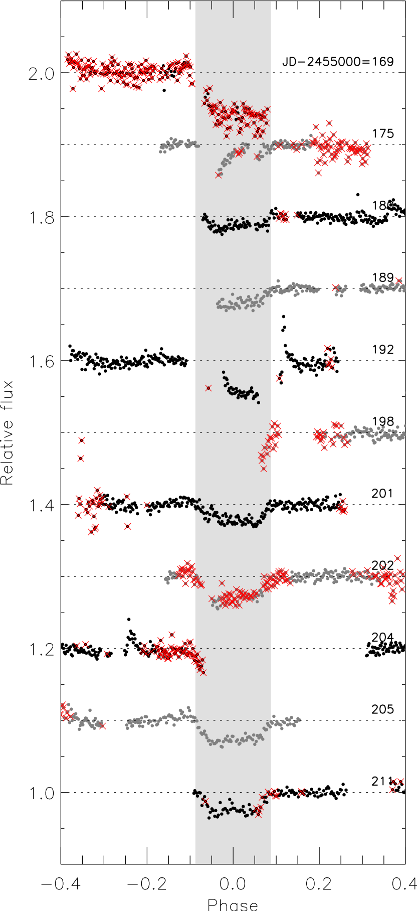
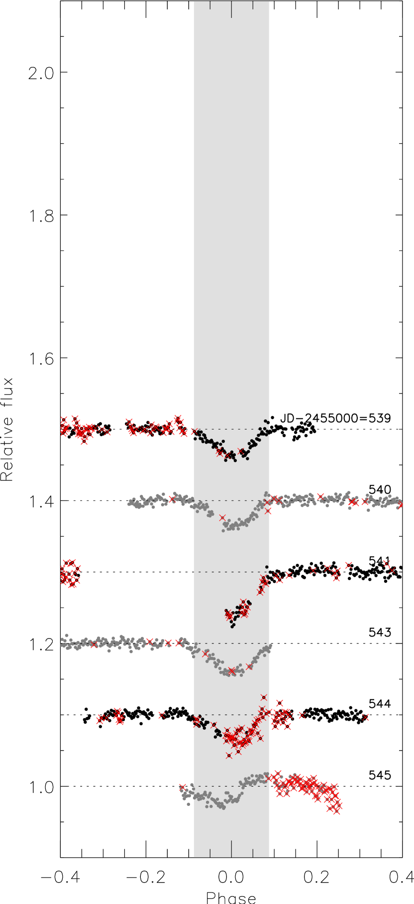
Figure 6: Whitened light curves for nights where in-transit data were obtained, folded on the transit period (Section 3.1.1; left and right panels show first and second year’s data respectively). Flux values are normalized to unity outside of eclipse, and nights are offset vertically in increments of 0.1 for clarity. Transits are further distinguished in alternating black and gray, and crosses (red in the online color version) indicate data flagged as potentially compromised. The Julian day on which each transit occurred is indicated for comparison with Figures 2 and 3. The light gray regions indicate the transit windows. Note that partially covered transits with little or no data on one or other side of the transit window are likely to suffer from poor stellar-variability correction and show significant systematic error.

The original “un-whitened” light curve is dominated by stellar variability (see Figures 2 and 3). If we assume that the large-scale variability is caused primarily by spot modulation, and that the relative effect of the transit events is negligible, we can use the un-whitened data to investigate the stellar rotation. Lomb-Scargle periodograms (Lomb 1976; Scargle 1982) of the two years’ data are shown in Figure 7. Where the Plavchan periodogram is designed for finding regular periodic features of arbitrary but constant shape (such as a transit), a Lomb-Scargle periodogram is better suited for finding periodic modes in a more complex signal such as the quasi-periodic stellar variation in our data: here, the signal appears not to repeat in an exact fashion and therefore does not fold well at any period (likely because of phase shifts due to changing spot features).

A strong peak is found at $0.4481\pm 0.0022\,{\rm d}$, in fact matching well with the transit period. Another peak is seen at $0.9985\pm 0.0061\,{\rm d}$, corresponding closely to the sidereal or solar Earth day, and therefore most likely an artifact resulting from the observing cadence. The other peaks all appear to be aliases of these two periods. To confirm this, we modeled the data by creating an artificial light curve from two summed sinusoids with the same two periods, providing power at the frequencies of these two peaks. We superimposed artificial transits modeled as a simple inverted top-hat function, with the same depth, width, and ephemeris as the real transits. Allowing the phases and relative amplitude of the $0.4481\,{\rm d}$ and $0.9985\,{\rm d}$ signals to vary as free parameters, and requiring that the total amplitude of the light curve remain approximately the same as that of the actual data, we performed a least-squares fit to the real periodogram to assess how well its structure could be reproduced. Figure 7 shows the results, with a good match between model and data. Repeating the test with the $0.4481\,{\rm d}$ sinusoid omitted (i.e., summing only the one-day signal and the transits) gave a poor fit, implying that the form of the periodogram cannot be explained by the transits alone. Since there is clearly strong correlated out-of-transit variability associated with the star, and there are no other fundamental periods evident in the periodogram, the $0.4481\,{\rm d}$ signal appears to be the only likely period for the star.

There are three other notable aliases of the presumed stellar rotation period, $P_{*}$, at $0.3092\pm 0.0010\,{\rm d}$, $0.8126\pm 0.0070\,{\rm d}$, and $4.43\pm 0.31\,{\rm d}$ (identified in the figure). The larger of these is substantially above the upper period limit implied by the measured $v_{\mathrm{r}}\sin i_{*}$ of the star (Section 3.2.2), $P_{*}<2\pi R_{*}/(v_{\mathrm{r}}\sin i_{*})=0.671\pm 0.092\,{\rm d}$. Though it is unlikely that the star would be coincidentally rotating at an alias of the transit period with the Earth’s rotation, we repeated the modeling experiment with the model stellar rotation modified to match the remaining two aliases to ensure that none could in fact be the true fundamental stellar period (see Dawson & Fabrycky 2010). Similar periodograms were obtained, with peaks at similar locations but with differing strength ratios; none were as good a fit to the periodograms based on the real data. We therefore conclude that the star is co-rotating or near co-rotating with the companion orbit.

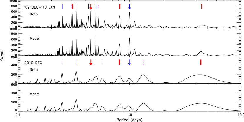
Figure 7: Lomb-Scargle periodogram of the non-whitened light curves from the two years of PTF Orion observations, compared to simple synthetic models (Section 3.1.1). The presumed stellar rotation period is marked with a thick arrow (red in the online color version); a second distinct one-day period, which we attribute to the observing cadence, is marked with a thin (blue) arrow. The more prominent aliases of these periods are indicated with vertical lines: thick (red) marks indicate peaks which are predominantly produced by aliases of the presumed stellar rotation period; thin (blue) marks indicate peaks predominantly produced by aliases of the one-day period. Dotted (magenta) lines indicate peaks produced by a combination of the two.

We note that it is difficult to model the observed transit events with star spots alone, particularly in the 2009 December/2010 January data: the short transit duration relative to the period, the flat bottom of the transits, and the sharp ingress and egress, are all more characteristic of a transiting object, whereas spots tend to cause smoother, more sinusoidal features as their projected area changes as they rotate across the stellar disk. It is more likely that we are seeing in the total lightcurve the effects of both star spots and a transiting object.

3.1.2 Transit Fitting

We fit transit models to the whitened light curves using the IDL-based Transit Analysis Package (TAP; Gazak et al. 2012). TAP employs Bayesian Markov Chain Monte Carlo (MCMC) techniques to explore the fitting parameter space based on the analytic transit light curve models of Mandel & Agol (2002). The package incorporates white- and red-noise parameterization (Carter & Winn 2009), allowing for robust estimates of parameter uncertainty distributions. We fit only the transits from nights where a complete transit was observed with adequate coverage both before and after the transit window, since on these nights the spline fit to remove the stellar variability is reasonably constrained on both sides of the transit; on nights where there is partial transit coverage, the spline fit tends to diverge during transit time. We also reject the transits mentioned in section 3.1 where stellar variability appears to strongly affect the shape of the transit, and in addition, the transit from JD 2455544, where the spline subtraction was particularly uncertain and rather sensitive to the tightness of the spline fit. Thus we fit four of the transits from the first year’s data (JDs 2455201, 2455202, 2455205, and 2455211), and three from the second year (JDs 2455539, 2455540, and 2455543). The folded data are shown in Figure 8.

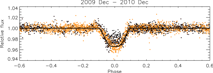
Figure 8: Folded light curve for the two years of observations combined, after removing stellar variability (Section 3.1.1). The first year’s data (2009 December – 2010 January) are plotted in black; the second year’s (2010 December) are plotted in orange. A change in transit shape between the two years is evident. The best transit fit to both years combined is over-plotted on the assumption that $R_{p}<R_{*}$ (Section 3.1.2). Limb darkening is neglected, and error bars are omitted for clarity; the median photometric error is 0.0046, with an out-of-eclipse standard deviation of 0.0056.

For the transit fitting, we hold the orbital period, $P$, fixed to the transit period determined above. The eccentricity, $e$, is fixed at zero, since it is difficult to constrain in the absence of a secondary eclipse. White and red noise levels are allowed to float separately for each individual transit, as are linear airmass trends. The remaining parameters are allowed to float, but are tied across all transits. They include: the epoch of transit center, $T_{0}$ (we assume there are no transit timing drifts between the two years); the orbital inclination, $i_{\mathrm{orb}}$; $a/R_{*}$, where $a$ is the orbital semi-major axis, and $R_{*}$ is the radius of the primary; $R_{\mathrm{p}}/R_{*}$, where $R_{\mathrm{p}}$ is the companion radius; and the linear and quadratic limb-darkening coefficients for the primary star. In addition, we constrain the fitting such that $R_{\mathrm{p}}/R_{*}<1$, and white and red noise components are less than 4% (the depth of the transit). Parameters are calculated by fitting Gaussians to the dominant peak in the probability density distributions for each parameter resulting from the MCMC analysis. The center location of the Gaussian is taken as the parameter value, and measurement errors are estimated as the dispersion of the fit. We find that the limb-darkening coefficients are largely unconstrained by the data. The fit is shown overlaid on the folded data in Figure 8; the corresponding parameters are listed in Table 3.

Table 3: System Parameters

Parameter	Value
Measured
$P$	$0.448413\pm 0.000040\,{\rm d}$
$i_{\mathrm{orb}}$	$61.8\pm 3.7\arcdeg$
$a/R_{*}$	$1.685\pm 0.064$
$R_{\mathrm{p}}/R_{*}$	$0.1838\pm 0.0097$
$T_{0}$ (HJD)	$2455543.9402\pm 0.0008$
$v_{\mathrm{r}}\sin i_{*}$	$80.6\pm 8.1\,{\rm km}\,{\rm s}^{-1}$
Derived
$a$	$0.00838\pm 0.00072\,{\rm AU}$
	$=1.80\pm 0.15\,{R_{\odot}}$
$R_{*}$	$1.07\pm 0.10\,{R_{\odot}}$
$R_{\mathrm{p}}$	$1.91\pm 0.21\,{R_{\mathrm{Jup}}}$
$M_{\mathrm{p}}\sin i_{\mathrm{orb}}$	$\leq 4.8\pm 1.2\,M_{\rm Jup}$
$M_{\mathrm{p}}$	$\leq 5.5\pm 1.4\,M_{\rm Jup}$

Note. — Summary of parameters determined in this paper for the PTFO 8-8695 system. Quantities are $P$ – orbital period; $i_{\mathrm{orb}}$ – orbital inclination; $i_{*}$ – inclination of stellar rotation axis; $a$ – orbital semi-major axis; $R_{*}$ – stellar radius; $R_{p}$ – planet radius; $T_{0}$ – epoch of transit center; $v_{\mathrm{r}}$ – stellar equatorial rotational velocity; $M_{\mathrm{p}}$ – planet mass.

There is significant variation in the light curve from transit to transit, as can be seen in Figure 6. This can reasonably be attributed to the companion passing across varying surface features – cold or hot spots, or perhaps flares – on the stellar photosphere. Such variations are a result of the planet tracing the stellar surface brightness profile as it traverses the stellar disk, and cannot be removed by the whitening process, which is only sensitive to the integrated brightness of the disk. Since PTFO 8-8695 is expected to be active and spotted, such variation in the transits is further suggestive of a genuine transit, rather than a background blend.

It can also clearly be seen from Figures 6 and 8, however, that there is an overall change in the transit shape between the two years’ data sets. Explanations for this remain speculative. Re-running the fitting process and allowing a change in both $R_{*}$ and $R_{\mathrm{p}}$ between the two years yields a decrease in stellar radius of $\approx 10$% $(2.1\sigma)$ from one year to the next (with no measurable change in companion radius). Such a large change in the stellar radius in such a short time period is unlikely, and would likely manifest itself in observable rotation rate changes not seen in the data. A change in transit shape could also arise in principle from a change in orbital geometry. For example, the host star is rotating quickly enough to exhibit significant oblateness, which may induce precession of the orbital plane and, therefore, changes in $i_{\mathrm{orb}}$ if the orbital and stellar rotational axes are misaligned. An additional planet in a different orbit could also produce a similar effect (Miralda-Escudé 2002). It is difficult, however, to explain how an inclination change can yield a transit that becomes both more grazing (longer ingress/egress) and deeper at the same time. Another explanation may be variation in star spot coverage (or limb-darkening, though with heavy spot coverage, the two effects become somewhat confused). In addition to short-term spot variations, there may be surface features which survive for much longer periods (see, e.g., Mahmud et al. 2011). Given the activity of the star and the extreme proximity of the companion, such features may be compounded by magnetic or tidal star/planet interactions that could give rise to varying hot or cold spots near the sub-planetary point on the stellar photosphere. This could affect the apparent shape of the transit in a systematic way. The planet’s apparent proximity to the tidal disruption limit (see section 3.3) may also be a factor: a tidally distorted shape, or transient rings or a tidal tail of evaporating material could all yield unexpected and possibly varying transit shape (and also cause the slight transit asymmetry seen in the second year’s data). For the sake of simplicity, and given the lack of data to disentangle all of these possibilities, we here adopt the single combined fit to both years’ data sets, although with the caveat that the variability may cause some systematic error in the measurements.

We note that our fit yields a somewhat smaller stellar radius, $R_{*}\approx 1.07\,{R_{\odot}}$, than that previously reported by Briceño et al. (2005) ($1.39\,{R_{\odot}}$). Assuming their estimate of $T_{\mathrm{eff}}=3470\,{\rm K}$ is correct, interpolating Siess models (Siess et al. 2000) with this updated radius gives a slightly older age estimate for the star, $\approx 3.7\,{\rm Myr}$ vs. $2.7\,{\rm Myr}$. Given the distance uncertainties in the Briceño et al. (2005) results, however, and the possibility of uncertainty in $T_{\mathrm{eff}}$ arising from heavy spotting in the stellar photosphere, the two radius estimates are probably not inconsistent.

3.2 Spectroscopy

3.2.1 Radial Velocities

Since the RV analysis is differential in nature, the RV offset between the HET and Keck data sets is arbitrary. We place them on the same approximate scale by shifting the RV zero points to the mean of the data for each data set. There are too few data points to create a periodogram to measure any periodicities in the data, but we can look for consistency with the previously determined transit period by folding the data on that period and looking for a coherent alignment of the data points. The result is shown in Figure 9: indeed, the data appear to phase well, showing a smooth and apparently sinusoidal variation, with the exception of one outlying data point at orbital phase $\phi=-0.082$ (Heliocentric Julian date (HJD) 2455615.64969), which is discussed further below. This outlier is excluded in calculating the offset between the data sets.

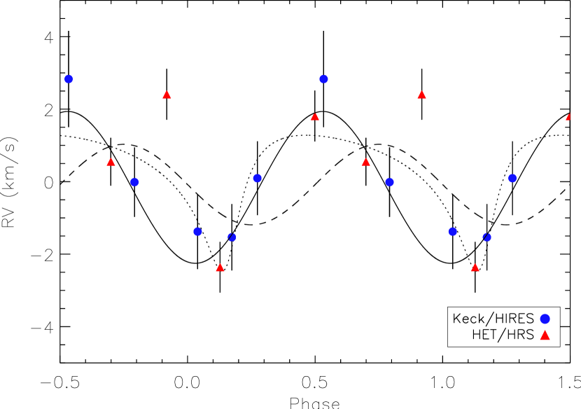
Figure 9: Differential radial velocity measurements obtained with Keck/HIRES and HET/HRS (Section 3.2.1). Zero phase is chosen to correspond to the photometric center-of-transit time. The offset between the two datasets is chosen to match the mean RV of each. The lines indicate best Keplerian fits (excluding the outlier): dashed line – circular orbit, transit-center time, $T_{0}$, fixed to photometry ($\chi^{2}_{\rm red}=4.0$); dotted line – eccentric orbit, transit-center time fixed to photometry ($\chi^{2}_{\rm red}=1.1$); solid line – a sinusoidal fit (equivalent to a circular orbit) at the same period, with phase free to float ($\chi^{2}_{\rm red}=0.42$). The eccentric fit is better than the fixed-$T_{0}$ fit, but brings the companion to the surface of the star at periastron. The floating-phase sinusoidal fit gives the best result, suggesting that star spots either modify or dominate the Doppler RV signal. The outlier point may represent Rossiter McLaughlin effect due to the transiting companion.

To constrain the mass of the companion, we fit a Keplerian orbit model to the data using the RVLIN package by Wright & Howard (2009). The model includes six parameters: the period, $P$; the RV semi-amplitude, $K$; the eccentricity, $e$; the argument of periastron, $\omega$; the time of periastron passage, $T_{\mathrm{p}}$; and the systemic velocity, $\gamma$. We fixed $P$ and $T_{\mathrm{p}}$ to the values measured from the transit photometry. Since the $\chi^{2}$ surface has multiple minima, we explore the fitting parameter space by running 10000 trial Keplerian fits (neglecting the apparent outlier point), with initial parameter estimates drawn at random from reasonable starting distributions, and selecting the fit with the lowest reduced $\chi^{2}$ ($\chi^{2}_{\rm red}$).

We find that the constraints from the transit ephemeris make it difficult to obtain a reasonable Keplerian fit. A good circular-orbit fit, with the eccentricity, $e$, fixed to zero, is prohibited by the constraint on $T_{0}$ provided by the photometry. Such a fit must cross its central velocity at phases 0 and 0.5, with minima and maxima at 0.25 and 0.75 (the quadrature points), and as a result appears significantly out of phase with the data ($\chi^{2}_{\rm red}=4.0$; dashed line, Figure 9).

An eccentric fit goes some way to resolving the mismatch ($\chi^{2}_{\rm red}=1.1$), but yields an eccentricity of $e\approx 0.492$ (dotted line, Figure 9). This places the fractional periastron distance at $r_{\mathrm{peri}}/a\equiv 1-e\approx 0.51$, bringing the companion to the point of contact with the surface of the star as determined from the photometric transit fits ($R_{*}/a\approx 0.51$). Such a solution may be improbable, given that in section 3.3 we note that the orbital semi-major axis appears to be close to the Roche limit.

A better fit is in fact obtained by fitting a circular orbit model and removing the constraint on $T_{0}$, allowing the phase to float. This fit is over-plotted in Figure 9, showing the fit is good ($\chi^{2}_{\rm red}=0.42$), but offset in phase from the transit ephemeris by $-0.22\pm 0.04$ periods.

We favor this better fit to the RV signal, which most likely arises because of spot effects modulated by the stellar rotation, where the amplitude of the spot effect is at least comparable to – if not much greater than – any true reflex Doppler signal from the companion. Similar spot-induced RV amplitudes have already been observed for other T-Tauri stars in the optical (e.g., Mahmud et al. 2011; Huerta et al. 2008; Prato et al. 2008). Since the star appears to be co-rotating with the planet orbit, the period of such a spot-dominated RV signal would match the orbital period, but the phase would be arbitrary, depending on the longitudinal spot placement. Alternatively, spot and companion RV signals may both be significant and the two effects may compete (see Section 3.3).

Regardless of the astrophysical cause behind the measured RV signal, we can place an upper limit on the companion mass, and because of the good orbital phase coverage we can be reasonably assured that possible aliasing effects are not a concern. We assume that any companion-induced Doppler motion must be smaller than the amplitude of the measured variations, that $M_{p}\ll M_{*}$, and that $M_{*}=0.39\pm 0.10\,M_{\odot}$ (Briceño et al. 2005), and hence estimate $M_{\mathrm{p}}\sin i_{\mathrm{orb}}\leq 4.8\pm 1.2\,M_{\rm Jup}$ (see, e.g., formula 3, Gaudi & Winn 2007). Taking our derived value of $i_{\mathrm{orb}}$ we can directly estimate $M_{\mathrm{p}}\leq 5.5\pm 1.4\,M_{\rm Jup}$, comfortably within the planetary mass regime. The semi-amplitude (half peak-to-peak) of the combined measured RV variations is $\approx 2.4\,{\rm km}\,{\rm s}^{-1}$. This is separately confirmed by the two individual datasets, which both have good phase coverage and show similar amplitudes independent of the RV offset (as can be seen in Figure 9). By comparison, since Doppler-induced RV semi-amplitude scales directly with $M_{\mathrm{p}}$, a $25\,M_{\rm Jup}$ object on the planet/brown-dwarf boundary suggested by Schneider et al. (2011) would induce an $11\,{\rm km}\,{\rm s}^{-1}$ signal; an object on the deuterium-burning limit ($\approx 13\,M_{\rm Jup}$) would induce a $5.7\,{\rm km}\,{\rm s}^{-1}$ signal. It is unlikely, therefore, that the object is of more than planetary mass, and still less in the stellar mass range. Since the spot distribution is likely to change with time, further observations to look for changes in the phase of the RV signal with respect to the transit ephemeris may provide more insight into the exact nature of the RV signal. RV observations in the infra red are also likely to suffer less from spot-induced noise, and so could also provide valuable further information.

We were unable to find any abnormalities in the observations regarding the outlying RV data point, and, thus, have no reason to reject it as a bad measurement. However, falling at an orbital phase $\phi=-0.082$, it lies within the transit window (c.f. Figure 8), and its anomalous velocity could reasonably be explained as arising from the Rossiter-McLaughlin (RM) effect (Rossiter 1924; McLaughlin 1924). The RM effect would appear regardless of whether the main RV signal is caused by spot modulation or stellar reflex motion, since it is a result of an asymmetric distortion of the stellar absorption lines as an obscuration transits the unresolved stellar disk, blocking off regions with successively different rotational red-shifts. Indeed, given the rapid stellar rotation, the RM effect should be expected to appear during the transit window. From equation 6 of Gaudi & Winn (2007) we can estimate the expected maximum amplitude of the effect, $K_{R}$, given $v_{\mathrm{r}}\sin i_{*}$, $R_{p}$, and $R_{*}$. We find $K_{R}\approx 3\,{\rm km}\,{\rm s}^{-1}$, in good agreement with the offset of the outlier. The RM maximum also lies typically around $\sim 1/5$–1/3 of the way between transit-ingress and transit-center for gas-giant planets, which is coincidentally where the outlier point is located. The sign of the offset of the outlier data point, falling prior to the transit center time, is in agreement with a prograde orbit, as we would expect if the star is in synchronous (or quasi-synchronous) rotation. It should be noted that the RV data point at $\phi=+0.039$ (HJD 2455671.755651) also lies within the transit window but, in contrast, does not appear to be an outlier. Lying closer to the transit center time, one would expect the RV offset to be smaller here; however, the exact form of the RM effect depends on the precise orbital geometry, and may be partially masked by the choice of offset between the two data sets. Further complication may also arise from the companion transiting photospheric surface features. Dedicated RV measurements during transit could provide valuable confirmation of the RM effect hinted at by the data, and help independently confirm the validity of the transiting planet candidate.

3.2.2 Stellar Rotation

The stellar rotation velocity, $v_{\mathrm{r}}$, measured from the spectroscopy provides an independent consistency check on the stellar rotation period. In order to estimate the projected rotation velocity, $v_{\mathrm{r}}\sin i_{*}$, we degrade the Kurucz synthetic model spectrum (see Section 2.4) to the resolution and sampling of the HRS, and rotationally broaden it using a non-linear limb-darkening model (Claret 2000; Gray 1992) over the range of $v_{\mathrm{r}}\sin i_{*}=10$ – $150\,{\rm km}\,{\rm s}^{-1}$. We then Doppler shift the broadened models, line by line, by cross-correlating against lines in our target spectrum. Subtracting a Doppler shifted model from the observed spectrum gives an RMS residual for that rotational velocity. Minimizing this residual gives the optimal rotational velocity measured for an individual line. We applied this analysis to 12 lines that were sufficiently deep to be visible above the noise for our full range of $v_{\mathrm{r}}\sin i_{*}$ models. Weak lines could not be used because at large $v_{\mathrm{r}}\sin i_{*}$ the line profiles became buried in the noise. The weighted average of $v_{\mathrm{r}}\sin i_{*}$ measured for these lines, across all four HRS observations, was $80.6\pm 8.1\,{\rm km}\,{\rm s}^{-1}$.

The assumed rotational period of the star and the radius measured from photometric transit fitting (neglecting oblateness effects) independently imply an expected value for the unprojected rotational velocity of $v_{\mathrm{r}}=2\pi R_{*}/P_{*}\approx 120\pm 11\,{\rm km}\,{\rm s}^{-1}$. Taken together, the measured $v_{\mathrm{r}}\sin i_{*}$ and the photometrically derived $v_{\mathrm{r}}$ give an estimated inclination of the stellar rotation axis, $i_{*}=42\pm 7\arcdeg$. Comparing this with the measured orbital inclination, $i_{\mathrm{orb}}=61.8\pm 3.7\arcdeg$, we see that there is weak evidence for a possible misalignment between the orbital and stellar rotation axes (consistent with the possibility of detecting changes in the orbital inclination on relatively short timescales, as mentioned in Section 3.1.2).

3.3 Implications

In Figure 10 we show the radius and mass of the companion in relation to the currently known transiting exoplanets listed in the NASA Exoplanet Archive, where we have indicated the mass of the candidate as an upper limit only. It clearly lies at the upper end of the gas-giant radius distribution, although not unprecedentedly so. A significantly inflated atmosphere is to be expected owing both to the system’s very young age, and to stellar irradiation at the companion’s exceptionally small orbital radius. Planetary atmosphere models are currently not well constrained in this regime due to the lack of known exoplanets that are both young and close-in. Marley et al. (2007) and Fortney et al. (2007) caution that evolutionary models should be treated with care at ages up to $10\,{\rm Myr}$ or more, being highly dependent on initial conditions and the formation mechanism assumed. Indeed, Spiegel & Burrows (2012) suggest that comparison of atmospheric models with observations of exoplanets at such young ages may be a good way of distinguishing between different formation scenarios. Both Spiegel & Burrows (2012) and Marley et al. (2007) predict radii of around $1.6\,{R_{\mathrm{Jup}}}$ for a $5\,M_{\rm Jup}$ planet at $3\,{\rm Myr}$, for non-irradiated ‘hot-start’ (gravitational collapse) model atmospheres; our error bars place our measured radius ($1.9\pm 0.2\,{R_{\odot}}$) just above this value. Our radius lies substantially further above the post-formation cold-start (core collapse) isochrones, though comparison with the latter models is confused by uncertainty in the formation timescale, which is likely comparable to the age of the star. Accounting for stellar irradiation could increase the theoretical radius further. Increases of $\sim 10\%$ or more are typical at $\sim 0.02\,{\rm AU}$ from a solar like star (Baraffe et al. 2010; Chabrier et al. 2004), where the incident flux is similar to that on our planet candidate (which is closer in, but orbiting a lower-mass star). The companion’s proximity to the Roche limit may also weaken the gravitational binding of the object, further increasing its expected radius. Various other explanations are also proposed to explain the excess “radius anomaly” that is increasingly found in other gas-giant exoplanets (e.g., Baraffe et al. 2010; Chabrier et al. 2011). Our estimated radius is therefore not unreasonable, but due to both the model and observation uncertainties, a robust comparison with theory is difficult.

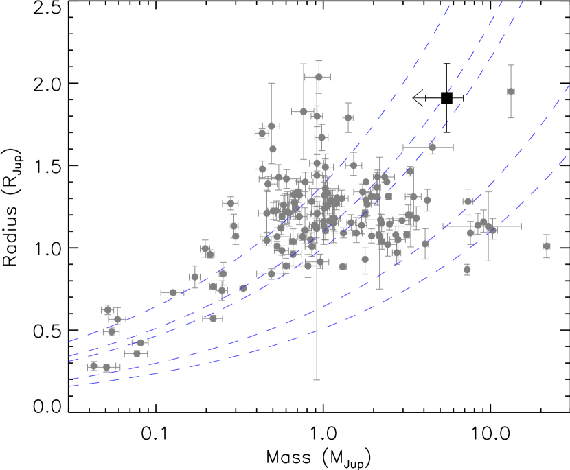
Figure 10: Radius vs. mass for the known transiting planets (Section 3.3; data taken from the NASA Exoplanet Archive). PTFO 8-8695b is marked as an upper mass limit, highlighted by the large square. Iso-density contours are marked at 0.5, 1, 1.33 (Jupiter density), 5, and $10\mathrm{\,g\,cm^{-3}}$.

The apparent companion to PTFO 8-8695 also orbits close enough to its parent star that the consequent small size of its Roche lobe may be relevant. Below a certain mass threshold, it may not have sufficient self-gravity to hold itself together, and thus may begin to lose mass. Following Faber et al. (2005) and Ford & Rasio (2006), the Roche radius, $R_{\mathrm{Roche}}$, according to Paczyński (1971), is given by

$$R_{\mathrm{Roche}}\;=\;0.462(M_{\mathrm{p}}/M_{*})^{1/3}a\;\leq\;0.462(M_{\mathrm{p,max}}/M_{*})^{1/3}a\;\approx\;1.92\pm 0.16,$$ (1)

where $M_{\mathrm{p,max}}$ is our previously estimated maximum mass for the companion. Comparing with the measured companion radius gives $R_{\mathrm{p}}/R_{\mathrm{Roche}}\gtrsim 0.994\pm 0.094$. Framing the argument another way, we can rewrite the Roche formula to estimate the Roche limiting orbital radius, $R_{\mathrm{Roche}}$, in terms of the measured companion radius to find $a/a_{\mathrm{Roche}}\lesssim 1.008\pm 0.095$ at the most – consistent with being at or within the Roche limit, within the errors. The planet may be sufficiently inflated that it fills its Roche lobe, and consequently may have lost mass in the past, or be in the process of losing mass (thus maintaining itself at the Roche limit).

4 Conclusions

We have detected transits from a candidate young planet orbiting a previously-identified co-rotating or near-co-rotating $\approx 2.7\,{\rm Myr}$-old M3 weak-line T-Tauri star. Although we cannot completely rule out a false positive due to source blends, we are able to rule out confusion at the level of $\Delta H\approx 4.3\,{\rm mag}$ beyond a separation of 0.25″, and argue qualitatively that a false detection due to a blended eclipsing binary is unlikely. The companion is in an exceptionally rapid $0.448413\,{\rm d}$ orbit, placing it among the shortest of the currently known exoplanet periods (cf. Demory et al. 2011; Charpinet et al. 2011; Muirhead et al. 2012; Rappaport et al. 2012). With an orbital radius only around twice the stellar radius, it appears to be at or within its Roche limiting orbit, with $a/a_{\mathrm{Roche}}\lesssim 1.01\pm 0.10$, raising the possibility of past or ongoing evaporation and mass loss. Perhaps the companion has been migrating, and losing any mass beyond its Roche lobe as it does so; or perhaps it is continually being inflated to fill its Roche lobe, with any material which overflows being stripped away.

Although the transit photometry and the RV data both phase-fold on the same periods, there is an apparent offset in phase between them. The most likely explanation is that the RV signal is shifted or dominated by the effect of star spots; we therefore suggest an upper limit on the (inclination independent) companion mass of $\approx 5\,M_{\rm Jup}$ based on the amplitude of the RV modulation. If it can be assumed that the object has had time to reach a stable (or quasi-stable) state – i.e., that mass loss rates are not too rapid, and that there have been no recent dramatic changes in the orbital geometry – then Roche limit considerations would imply a lower limit of a similar order, since anything much less would be unable to gravitationally bind the material within the measured companion radius.

The data are complex enough that we cannot yet be certain of a planet detection. In favor of the planetary interpretation, however, we note that: (1) the photometric transit shape appears to be flat bottomed with sharp ingress and egress slopes, and is difficult to explain with a star-spot model alone; (2) the transits appear highly consistent and periodic over a period of $\gtrsim 1\,\mathrm{yr}$, which would be unusual for spots; (3) the RV signal places an upper mass limit well within the planetary regime; (4) a false positive due to a faint blended eclipsing binary is argued against by two observations which are suggestive of a transiting object associated with the primary T-Tauri star observed: the stellar rotation rate appears very close to the transit period, suggesting co-rotation; and the photometric variation from transit to transit is consistent with the notion of a planet transiting a heavily spotted T-Tauri star.

Further spectroscopic and photometric observations are needed to provide a clearer picture. Since the star is such a fast rotator, the expected RM effect (hinted at in the data) may provide a valuable opportunity for confirmation of the candidate. Most RV noise sources will be constant in the timescale of one transit, so further RV observations during the transit window could potentially provide full sampling of the effect. This would help confirm the planetary interpretation of the data, and could provide further useful information on the system geometry. Revisiting the target to make further measurements of the RV phase with respect to the transit ephemeris would help confirm the spot-interference interpretation: if spots are significant, the phase offset is likely to change with time as the spots change. Infra-red RV observations, which are less sensitive to spot-induced noise, would also provide valuable further information, perhaps allowing for an unambiguous determination of the companion mass.

Given the young age of the system, the planet candidate is likely hot, and so a secondary transit may also be detectable with more precise photometry, allowing constraints to be placed on the companion temperature. Finally, simultaneous multi-band photometry and spectroscopy (particularly in the infra-red, where spot-effects should be lessened) could further help disentangle the signatures of star spots and companion. This would also help to establish the cause of the apparent overall change in transit shape between the two years’ observing runs, which could result either from changes in the spot distribution or possibly, given the exceptionally short orbital timescale, changes in the orbital geometry.

If our interpretation of the data is correct, the putative planet’s youth and its unique proximity to its host star will make it a valuable object for helping inform our understanding of exoplanet formation. Its young age could have important implications for the mechanism by which it formed: conventional core-accretion formation models (Pollack et al. 1996) occur on timescales of $\sim 1$–$10\,{\rm Myr}$, comparable with or longer than the age of the system; the much more rapid gravitational-instability mechanism (Boss 1997, 2000) occurs on timescales orders of magnitudes shorter, and may thus perhaps be favored (see Baraffe et al. 2010, for a brief overview and comparison of the two mechanisms). The companion’s inflated atmosphere appears indicative of the “hot start” models of Marley et al. (2007) and Spiegel & Burrows (2012), which are associated with gravitational instability. At the same time, we cannot rule out that formation may yet be incomplete given the young age of the system. Neither can we rule out that the companion may be on the verge of evaporation and may not survive the lifetime of the star. Indeed, very few large planets are known to orbit small stars, and this object may well be transient. Much ambiguity remains at these young ages, and more observation and analysis of the system is needed. If the planetary nature of the proposed companion is confirmed, the system could provide a wealth of new information for constraining dynamical and atmospheric evolution models for exoplanets. We therefore propose PTFO 8-8695 as an object worthy of further careful study by the community.

References

- Agüeros et al. (2011) Agüeros, M. A., Covey, K. R., Lemonias, J. J., Law, N. M., Kraus, A., Batalha, N., Bloom, J. S., Cenko, S. B., Kasliwal, M. M., Kulkarni, S. R., Nugent, P. E., Ofek, E. O., Poznanski, D., & Quimby, R. M. 2011, ApJ, 740, 110
- Aigrain et al. (2007) Aigrain, S., Hodgkin, S., Irwin, J., Hebb, L., Irwin, M., Favata, F., Moraux, E., & Pont, F. 2007, MNRAS, 375, 29
- Armitage (2009) Armitage, P. J. 2009, in American Institute of Physics Conference Series, Vol. 1192, American Institute of Physics Conference Series, ed. F. Roig, D. Lopes, R. de La Reza, & V. Ortega, 3–42
- Baraffe et al. (1998) Baraffe, I., Chabrier, G., Allard, F., & Hauschildt, P. H. 1998, A&A, 337, 403
- Baraffe et al. (2010) Baraffe, I., Chabrier, G., & Barman, T. 2010, Reports on Progress in Physics, 73, 016901
- Bender et al. (2012) Bender, C. F., Mahadevan, S., Deshpande, R., Wright, J. T., Roy, A., Terrien, R. C., Sigurdsson, S., Ramsey, L. W., Schneider, D. P., & Fleming, S. W. 2012, ApJ, 751, L31
- Boss (1997) Boss, A. P. 1997, Science, 276, 1836
- Boss (2000) —. 2000, ApJ, 536, L101
- Briceño et al. (2005) Briceño, C., Calvet, N., Hernández, J., Vivas, A. K., Hartmann, L., Downes, J. J., & Berlind, P. 2005, AJ, 129, 907
- Briceño et al. (2007) Briceño, C., Hartmann, L., Hernández, J., Calvet, N., Vivas, A. K., Furesz, G., & Szentgyorgyi, A. 2007, ApJ, 661, 1119
- Carter & Winn (2009) Carter, J. A. & Winn, J. N. 2009, ApJ, 704, 51
- Chabrier et al. (2004) Chabrier, G., Barman, T., Baraffe, I., Allard, F., & Hauschildt, P. H. 2004, ApJ, 603, L53
- Chabrier et al. (2011) Chabrier, G., Leconte, J., & Baraffe, I. 2011, in IAU Symposium, Vol. 276, IAU Symposium, ed. A. Sozzetti, M. G. Lattanzi, & A. P. Boss, 171–180
- Charpinet et al. (2011) Charpinet, S., Fontaine, G., Brassard, P., Green, E. M., van Grootel, V., Randall, S. K., Silvotti, R., Baran, A. S., Østensen, R. H., Kawaler, S. D., & Telting, J. H. 2011, Nature, 480, 496
- Claret (2000) Claret, A. 2000, A&A, 363, 1081
- Crockett et al. (2011) Crockett, C. J., Mahmud, N. I., Prato, L., Johns-Krull, C. M., Jaffe, D. T., & Beichman, C. A. 2011, ApJ, 735, 78
- Dawson & Fabrycky (2010) Dawson, R. I. & Fabrycky, D. C. 2010, ApJ, 722, 937
- Demory et al. (2011) Demory, B.-O., Gillon, M., Deming, D., Valencia, D., Seager, S., Benneke, B., Lovis, C., Cubillos, P., Harrington, J., Stevenson, K. B., Mayor, M., Pepe, F., Queloz, D., Ségransan, D., & Udry, S. 2011, A&A, 533, A114
- Esposito et al. (2006) Esposito, M., Guenther, E., Hatzes, A. P., & Hartmann, M. 2006, in Tenth Anniversary of 51 Peg-b: Status of and prospects for hot Jupiter studies, ed. L. Arnold, F. Bouchy, & C. Moutou, 127–134
- Faber et al. (2005) Faber, J. A., Rasio, F. A., & Willems, B. 2005, Icarus, 175, 248
- Ford & Rasio (2006) Ford, E. B. & Rasio, F. A. 2006, ApJ, 638, L45
- Fortney et al. (2007) Fortney, J. J., Marley, M. S., & Barnes, J. W. 2007, ApJ, 659, 1661
- Fortney & Nettelmann (2010) Fortney, J. J. & Nettelmann, N. 2010, Space Sci. Rev., 152, 423
- Gaudi & Winn (2007) Gaudi, B. S. & Winn, J. N. 2007, ApJ, 655, 550
- Gazak et al. (2012) Gazak, J. Z., Johnson, J. A., Tonry, J., Dragomir, D., Eastman, J., Mann, A. W., & Agol, E. 2012, Advances in Astronomy, 2012, 697967
- Gray (1992) Gray, D. F. 1992, The Observation and Analysis of Stellar Photospheres, 2nd edn. (Cambridge; New York: Cambridge University Press)
- Heacox (1987) Heacox, W. D. 1987, Journal of the Optical Society of America A, 4, 488
- Hernández et al. (2007) Hernández, J., Calvet, N., Briceño, C., Hartmann, L., Vivas, A. K., Muzerolle, J., Downes, J., Allen, L., & Gutermuth, R. 2007, ApJ, 671, 1784
- Hillenbrand (2008) Hillenbrand, L. A. 2008, Physica Scripta Volume T, 130, 014024
- Howard et al. (2009) Howard, A. W., Johnson, J. A., Marcy, G. W., Fischer, D. A., Wright, J. T., Henry, G. W., Giguere, M. J., Isaacson, H., Valenti, J. A., Anderson, J., & Piskunov, N. E. 2009, ApJ, 696, 75
- Huerta et al. (2008) Huerta, M., Johns-Krull, C. M., Prato, L., Hartigan, P., & Jaffe, D. T. 2008, ApJ, 678, 472
- Kraus & Ireland (2012) Kraus, A. L. & Ireland, M. J. 2012, ApJ, 745, 5
- Kurucz (2005) Kurucz, R. L. 2005, Memorie della Societa Astronomica Italiana Supplementi, 8, 14
- Law et al. (2010) Law, N. M., Dekany, R. G., Rahmer, G., Hale, D., Smith, R., Quimby, R., Ofek, E. O., Kasliwal, M., Zolkower, J., Velur, V., Henning, J., Bui, K., McKenna, D., Nugent, P., Jacobsen, J., Walters, R., Bloom, J., Surace, J., Grillmair, C., Laher, R., Mattingly, S., & Kulkarni, S. 2010, in Society of Photo-Optical Instrumentation Engineers (SPIE) Conference Series, Vol. 7735, Society of Photo-Optical Instrumentation Engineers (SPIE) Conference Series, 77353M
- Law et al. (2009) Law, N. M., Kulkarni, S. R., Dekany, R. G., Ofek, E. O., Quimby, R. M., Nugent, P. E., Surace, J., Grillmair, C. C., Bloom, J. S., Kasliwal, M. M., Bildsten, L., Brown, T., Cenko, S. B., Ciardi, D., Croner, E., Djorgovski, S. G., van Eyken, J., Filippenko, A. V., Fox, D. B., Gal-Yam, A., Hale, D., Hamam, N., Helou, G., Henning, J., Howell, D. A., Jacobsen, J., Laher, R., Mattingly, S., McKenna, D., Pickles, A., Poznanski, D., Rahmer, G., Rau, A., Rosing, W., Shara, M., Smith, R., Starr, D., Sullivan, M., Velur, V., Walters, R., & Zolkower, J. 2009, PASP, 121, 1395
- Levitan et al. (2011) Levitan, D., Fulton, B. J., Groot, P. J., Kulkarni, S. R., Ofek, E. O., Prince, T. A., Shporer, A., Bloom, J. S., Cenko, S. B., Kasliwal, M. M., Law, N. M., Nugent, P. E., Poznanski, D., Quimby, R. M., Horesh, A., Sesar, B., & Sternberg, A. 2011, ApJ, 739, 68
- Lomb (1976) Lomb, N. R. 1976, Ap&SS, 39, 447
- Mahmud et al. (2011) Mahmud, N. I., Crockett, C. J., Johns-Krull, C. M., Prato, L., Hartigan, P. M., Jaffe, D. T., & Beichman, C. A. 2011, ApJ, 736, 123
- Mandel & Agol (2002) Mandel, K. & Agol, E. 2002, ApJ, 580, L171
- Marley et al. (2007) Marley, M. S., Fortney, J. J., Hubickyj, O., Bodenheimer, P., & Lissauer, J. J. 2007, ApJ, 655, 541
- Marsh et al. (2010) Marsh, K. A., Kirkpatrick, J. D., & Plavchan, P. 2010, ApJ, 709, L158
- McLaughlin (1924) McLaughlin, D. B. 1924, ApJ, 60, 22
- Miller et al. (2008) Miller, A. A., Irwin, J., Aigrain, S., Hodgkin, S., & Hebb, L. 2008, MNRAS, 387, 349
- Miralda-Escudé (2002) Miralda-Escudé, J. 2002, ApJ, 564, 1019
- Muirhead et al. (2012) Muirhead, P. S., Johnson, J. A., Apps, K., Carter, J. A., Morton, T. D., Fabrycky, D. C., Pineda, J. S., Bottom, M., Rojas-Ayala, B., Schlawin, E., Hamren, K., Covey, K. R., Crepp, J. R., Stassun, K. G., Pepper, J., Hebb, L., Kirby, E. N., Howard, A. W., Isaacson, H. T., Marcy, G. W., Levitan, D., Diaz-Santos, T., Armus, L., & Lloyd, J. P. 2012, ApJ, 747, 144
- Neuhäuser et al. (2011) Neuhäuser, R., Errmann, R., Berndt, A., Maciejewski, G., Takahashi, H., Chen, W. P., Dimitrov, D. P., Pribulla, T., Nikogossian, E. H., Jensen, E. L. N., Marschall, L., Wu, Z.-Y., Kellerer, A., Walter, F. M., Briceño, C., Chini, R., Fernandez, M., Raetz, S., Torres, G., Latham, D. W., Quinn, S. N., Niedzielski, A., Bukowiecki, Ł., Nowak, G., Tomov, T., Tachihara, K., Hu, S. C.-L., Hung, L. W., Kjurkchieva, D. P., Radeva, V. S., Mihov, B. M., Slavcheva-Mihova, L., Bozhinova, I. N., Budaj, J., Vaňko, M., Kundra, E., Hambálek, Ľ., Krushevska, V., Movsessian, T., Harutyunyan, H., Downes, J. J., Hernandez, J., Hoffmeister, V. H., Cohen, D. H., Abel, I., Ahmad, R., Chapman, S., Eckert, S., Goodman, J., Guerard, A., Kim, H. M., Koontharana, A., Sokol, J., Trinh, J., Wang, Y., Zhou, X., Redmer, R., Kramm, U., Nettelmann, N., Mugrauer, M., Schmidt, J., Moualla, M., Ginski, C., Marka, C., Adam, C., Seeliger, M., Baar, S., Roell, T., Schmidt, T. O. B., Trepl, L., Eisenbeiß, T., Fiedler, S., Tetzlaff, N., Schmidt, E., Hohle, M. M., Kitze, M., Chakrova, N., Gräfe, C., Schreyer, K., Hambaryan, V. V., Broeg, C. H., Koppenhoefer, J., & Pandey, A. K. 2011, Astronomische Nachrichten, 332, 547
- Nguyen et al. (2012) Nguyen, D. C., Brandeker, A., van Kerkwijk, M. H., & Jayawardhana, R. 2012, ApJ, 745, 119
- Ofek et al. (2012) Ofek, E. O., Laher, R., Law, N., Surace, J., Levitan, D., Sesar, B., Horesh, A., Poznanski, D., van Eyken, J. C., Kulkarni, S. R., Nugent, P., Zolkower, J., Walters, R., Sullivan, M., Agüeros, M., Bildsten, L., Bloom, J., Cenko, S. B., Gal-Yam, A., Grillmair, C., Helou, G., Kasliwal, M. M., & Quimby, R. 2012, PASP, 124, 62
- Paczyński (1971) Paczyński, B. 1971, ARA&A, 9, 183
- Paulson & Yelda (2006) Paulson, D. B. & Yelda, S. 2006, PASP, 118, 706
- Plavchan et al. (2008) Plavchan, P., Jura, M., Kirkpatrick, J. D., Cutri, R. M., & Gallagher, S. C. 2008, ApJS, 175, 191
- Pollack et al. (1996) Pollack, J. B., Hubickyj, O., Bodenheimer, P., Lissauer, J. J., Podolak, M., & Greenzweig, Y. 1996, Icarus, 124, 62
- Prato et al. (2008) Prato, L., Huerta, M., Johns-Krull, C. M., Mahmud, N., Jaffe, D. T., & Hartigan, P. 2008, ApJ, 687, L103
- Ramsey et al. (1998) Ramsey, L. W., Adams, M. T., Barnes, T. G., Booth, J. A., Cornell, M. E., Fowler, J. R., Gaffney, N. I., Glaspey, J. W., Good, J. M., Hill, G. J., Kelton, P. W., Krabbendam, V. L., Long, L., MacQueen, P. J., Ray, F. B., Ricklefs, R. L., Sage, J., Sebring, T. A., Spiesman, W. J., & Steiner, M. 1998, in Society of Photo-Optical Instrumentation Engineers (SPIE) Conference Series, Vol. 3352, Society of Photo-Optical Instrumentation Engineers (SPIE) Conference Series, ed. L. M. Stepp, 34–42
- Rappaport et al. (2012) Rappaport, S., Levine, A., Chiang, E., El Mellah, I., Jenkins, J., Kalomeni, B., Kite, E. S., Kotson, M., Nelson, L., Rousseau-Nepton, L., & Tran, K. 2012, ApJ, 752, 1
- Rau et al. (2009) Rau, A., Kulkarni, S. R., Law, N. M., Bloom, J. S., Ciardi, D., Djorgovski, G. S., Fox, D. B., Gal-Yam, A., Grillmair, C. C., Kasliwal, M. M., Nugent, P. E., Ofek, E. O., Quimby, R. M., Reach, W. T., Shara, M., Bildsten, L., Cenko, S. B., Drake, A. J., Filippenko, A. V., Helfand, D. J., Helou, G., Howell, D. A., Poznanski, D., & Sullivan, M. 2009, PASP, 121, 1334
- Rossiter (1924) Rossiter, R. A. 1924, ApJ, 60, 15
- Scargle (1982) Scargle, J. D. 1982, ApJ, 263, 835
- Schneider et al. (2011) Schneider, J., Dedieu, C., Le Sidaner, P., Savalle, R., & Zolotukhin, I. 2011, A&A, 532, A79
- Setiawan et al. (2008) Setiawan, J., Henning, T., Launhardt, R., Müller, A., Weise, P., & Kürster, M. 2008, Nature, 451, 38
- Setiawan et al. (2007) Setiawan, J., Weise, P., Henning, T., Launhardt, R., Müller, A., & Rodmann, J. 2007, ApJ, 660, L145
- Shetrone et al. (2007) Shetrone, M., Cornell, M. E., Fowler, J. R., Gaffney, N., Laws, B., Mader, J., Mason, C., Odewahn, S., Roman, B., Rostopchin, S., Schneider, D. P., Umbarger, J., & Westfall, A. 2007, PASP, 119, 556
- Siess et al. (2000) Siess, L., Dufour, E., & Forestini, M. 2000, A&A, 358, 593
- Skrutskie et al. (2006) Skrutskie, M. F., Cutri, R. M., Stiening, R., Weinberg, M. D., Schneider, S., Carpenter, J. M., Beichman, C., Capps, R., Chester, T., Elias, J., Huchra, J., Liebert, J., Lonsdale, C., Monet, D. G., Price, S., Seitzer, P., Jarrett, T., Kirkpatrick, J. D., Gizis, J. E., Howard, E., Evans, T., Fowler, J., Fullmer, L., Hurt, R., Light, R., Kopan, E. L., Marsh, K. A., McCallon, H. L., Tam, R., Van Dyk, S., & Wheelock, S. 2006, AJ, 131, 1163
- Spiegel & Burrows (2012) Spiegel, D. S. & Burrows, A. 2012, ApJ, 745, 174
- Tull (1998) Tull, R. G. 1998, in Society of Photo-Optical Instrumentation Engineers (SPIE) Conference Series, Vol. 3355, Society of Photo-Optical Instrumentation Engineers (SPIE) Conference Series, ed. S. D’Odorico, 387–398
- van Eyken et al. (2011) van Eyken, J. C., Ciardi, D. R., Rebull, L. M., Stauffer, J. R., Akeson, R. L., Beichman, C. A., Boden, A. F., von Braun, K., Gelino, D. M., Hoard, D. W., Howell, S. B., Kane, S. R., Plavchan, P., Ramírez, S. V., Bloom, J. S., Cenko, S. B., Kasliwal, M. M., Kulkarni, S. R., Law, N. M., Nugent, P. E., Ofek, E. O., Poznanski, D., Quimby, R. M., Grillmair, C. J., Laher, R., Levitan, D., Mattingly, S., & Surace, J. A. 2011, AJ, 142, 60
- Vogt et al. (1994) Vogt, S. S., Allen, S. L., Bigelow, B. C., Bresee, L., Brown, B., Cantrall, T., Conrad, A., Couture, M., Delaney, C., Epps, H. W., Hilyard, D., Hilyard, D. F., Horn, E., Jern, N., Kanto, D., Keane, M. J., Kibrick, R. I., Lewis, J. W., Osborne, J., Pardeilhan, G. H., Pfister, T., Ricketts, T., Robinson, L. B., Stover, R. J., Tucker, D., Ward, J., & Wei, M. Z. 1994, in Society of Photo-Optical Instrumentation Engineers (SPIE) Conference Series, Vol. 2198, Society of Photo-Optical Instrumentation Engineers (SPIE) Conference Series, ed. D. L. Crawford & E. R. Craine, 362
- Wright & Howard (2009) Wright, J. T. & Howard, A. W. 2009, ApJS, 182, 205