Preliminary remarks on
option pricing and dynamic hedging

Abstract

An elementary arbitrage principle and the existence of trends in financial time series, which is based on a theorem published in 1995 by P. Cartier and Y. Perrin, lead to a new understanding of option pricing and dynamic hedging. Intricate problems related to violent behaviors of the underlying, like the existence of jumps, become then quite straightforward by incorporating them into the trends. Several convincing computer experiments are reported.
 
    Keywords— Quantitative finance, option pricing, European option, dynamic hedging, replication, arbitrage, time series, trends, volatility, abrupt changes, model-free control, nonstandard analysis.

I Introduction

Option pricing intends like many other financial techniques to tame as much as possible market risks. The Black-Scholes-Merton (BSM) approach ([7, 39]), which is forty years old, is still by far the most popular setting, although some of its drawbacks and pitfalls were known shortly after its publication. It had an enormous impact on the huge development of modern quantitative finance. Its heavy use of advanced mathematical tools, like stochastic differential equations and partial differential equations, explains to a large part the features of today’s mathematical finance, which is enjoying a great popularity not only among academics but also among practitioners. Many textbooks (see, e.g., [12, 13, 16, 26, 30, 34, 42, 50]) provide an excellent overview of this lively and fascinating field.

Let us add in the context of this conference that a growing number of references exploits the connections of the BSM setting with methods stemming from various engineering fields. We mention here:

• learning techniques (see, e.g., [27, 31]),

• control theory (see, e.g., [2, 4, 10, 14, 37, 41, 43, 49]).

In 1997, Scholes and Merton won the Nobel Prize in economics – Black died in 1995 – not for the discovery of the pricing formulas which were already known ([8, 44, 45, 48]), but for the methods they introduced for deriving them. The most elegant concepts of replication and dynamic delta hedging, which are now central both in theory and practice, have nevertheless been the subject of severe criticisms for their lack of realism (see, e.g., [15]). Dynamic delta hedging moreover cannot be extended to more general stochastic processes exhibiting jumps for instance ([40]).

Pricing formulas are derived here via an elementary arbitrage principle which employs the expected return of the underlying and goes back at least to [1] and [9]. Combined with the utilization of trends ([19]) it permits to

1. alleviate one of the most annoying paradoxes in modern approaches that concerns the uselessness of the expected return of the underlying (see, e.g., [6]),

2. deal quite simply with more subtle behaviors of the underlying, which may exhibit jumps, by incorporating those behaviors in the trends,

3. define a new more realistic dynamic hedging.

Our paper is organized as follows. Section II summarizes and sometimes improves some facts already presented earlier (see [22] and the references therein). Section III recalls how pricing formulas may be derived via an elementary arbitrage principle, i.e., without replication. Section IV slightly modifies those formulas by taking trends into account. A new dynamic hedging, which employs both the pricing formulas and the trend of the underlying, is proposed in Section V. Due to an obvious lack of space, the convincing computer illustrations, which are displayed in Section VI, are limited to a quite violent behavior of the underlying. Section VII further analyzes the change of paradigm which might arise from this new setting.

II The Cartier-Perrin theorem and some of its consequences: A short review

II-A Trend

The theorem due to Cartier and Perrin [11] is expressed in the language of nonstandard analysis. It depends on a time sampling $\mathfrak{TS}$ where the difference $t_{\nu+1}-t_{\nu}$ is infinitesimal, i.e., “very small”. Then, under a mild integrability condition, the price $S(t)$ of the financial quantity may be decomposed ([19]) in the following way

$$\boxed{S(t)=S_{\tiny{{\mathfrak{TS}},{\rm trend}}}(t)+S_{\tiny{{\mathfrak{TS}},{\rm fluct}}}(t)}$$

where

• $S_{\tiny{{\mathfrak{TS}},{\rm trend}}}$ is the trend, or the mean, or the average, of $S$;

• $S_{\tiny{{\mathfrak{TS}},{\rm fluct}}}$ is a quickly fluctuating function around $0$, i.e., $\int_{\tau_{0}}^{\tau_{1}}S_{\tiny{{\mathfrak{TS}},{\rm fluct}}}(\tau)d\tau$ is infinitesimal for any finite interval $[\tau_{0},\tau_{1}]$,

• $S_{\tiny{{\mathfrak{TS}},{\rm trend}}}$ and $S_{\tiny{{\mathfrak{TS}},{\rm fluct}}}$ are unique up to an additive infinitesimal quantity.

Remark II.1

$S_{\tiny{{\mathfrak{TS}},{\rm trend}}}(t)$, which is “smoother” than $S(t)$, provides a mathematical justification ([19]) of the trends in technical analysis (see, e.g., [3, 32]).

Remark II.2

Note that $S_{\tiny{{\mathfrak{TS}},{\rm fluct}}}(t)$ is analogous to “noises” in engineering according to the analysis of [17]. See [25] and [36] for the estimation of $S_{\tiny{\rm trend}}(t)$ and of its derivatives. See [22], and the references therein, for convincing numerical experiments including forecasting results which are deduced from the trends.

II-B Return

If $S_{\tiny{{\mathfrak{TS}},{\rm trend}}}$ is differentiable at $t$, then its logarithmic derivative

$${\mathbf{r}}_{{\tiny{{\mathfrak{TS}}}}{,{\rm trend}}}(t)=\frac{\dot{S}_{\tiny{{\mathfrak{TS}},{\rm trend}}}(t)}{S_{\tiny{{\mathfrak{TS}},{\rm trend}}}(t)}$$ (1)

is called the trend-return of $S$ at $t$.

Remark II.3

See [21, 22] for other definitions of returns.

II-C Volatility

Take two integrable time series $S_{1}(t)$, $S_{2}(t)$, such that their squares and the squares of $S_{1,\tiny{\rm trend}}(t)$ and $S_{2,\tiny{\rm trend}}(t)$ are also integrable. It leads us to the following definitions, which are borrowed from [21, 22]:

1. The covariance of two time series $S_{1}(t)$ and $S_{2}(t)$ is the time series

   $$\mbox{\rm cov}(S_{1}S_{2})(t) = {\mathrm{Tr}}\left((S_{1}-{\mathrm{Tr}}(S_{1}))(S_{2}-{\mathrm{Tr}}(S_{2}))\right)(t)$$

   $$\simeq {\mathrm{Tr}}(S_{1}S_{2})(t)-{\mathrm{Tr}}(S_{1})(t)\times{\mathrm{Tr}}(S_{2})(t)$$

   where ${\mathrm{Tr}}(\bullet)$ denotes the trend with respect to the time sampling $\mathfrak{TS}$.

2. The variance of the time series $S_{1}(t)$ is

   $$\mbox{\rm var}(S_{1})(t) = {\mathrm{Tr}}\left((S_{1}-{\mathrm{Tr}}(S_{1}))^{2}\right)(t)$$

   $$\simeq {\mathrm{Tr}}(S_{1}^{2})(t)-\left({\mathrm{Tr}}(S_{1})(t)\right)^{2}$$

3. The volatility of $S_{1}(t)$ is the corresponding standard deviation

   $$\mbox{\rm vol}(S_{1})(t)=\sqrt{\mbox{\rm var}(S_{1})(t)}$$ (2)

III Pricing without trends

We limit ourselves for simplicity’s sake to European call options, which are options for the right to buy a stock or an index at a certain price at a certain maturity date.

III-A Arbitrage

Let $r(t)$ be the risk-free rate. The expected price at maturity $T$ should be equal to

$$S(0)\exp\left(\int_{0}^{T}r(\tau)d\tau\right)$$ (3)

A heuristic justification goes like this: Assume, for simplicity’s sake and like in today’s academic literature, that

• $r(t)$ is a constant $r$,

• $S(t)$ follows a geometric Brownian motion

  $$S(t)=S(0)\exp\left[\left(\mu-\frac{\sigma^{2}}{2}\right)t+\sigma W(t)\right]$$ (4)

  where

  • $W(t)$ is a standard Brownian motion,

  • $\mu$ and $\sigma$ are constant.

Providing a theoretical estimation of $\mu$ and $\sigma$ from historical data is classic and straightforward. We thus know the mean $S(0)e^{\mu t}$ of $S(t)$. If $\mu>r$ (resp. $\mu<r$), it might be profitable for the arbitrageur to borrow money (resp. selling the underlying) for buying the underlying $S$ (resp. for investing the corresponding amount of money) at time $0$, and selling it (resp. buying the underlying) later, at time $T$ for instance.

III-B Formulas

Assume that

• the underlying follows the geometric Brownian motion (4),

• the expected final price satisfies the condition (3), i.e., is equal to

  $$S(0)e^{rT}$$

Krouglov [33] shows, by exploiting properties of log-normal distributions, that the usual BSM formulas may be recovered. Write down here the value of a European call option:

$$C(S,t)=S(t)N(d_{1})-KN(d_{2})e^{-r(T-t)}$$ (5)

where

• $N$ is the standard normal cumulative distribution function, i.e.,

  $$N(x)=\frac{1}{\sqrt{2\pi}}\int_{-\infty}^{x}\exp\left(-\frac{z^{2}}{2}\right)dz$$

• $K$ is the strike price,

• $d_{1}=\frac{\lg\left(\frac{S}{K}\right)+\left(r+\frac{\sigma^{2}}{2}\right)(T-t)}{\sigma\sqrt{T-t}}$,

• $d_{2}=d_{1}-\sigma\sqrt{T-t}$.

IV Pricing with trends

IV-A Arbitrage

Assume again that the risk-free rate $r(t)$ is a constant $r$. A natural extension of Section III states that the expected final price at maturity $T$ of the underlying is

$$S_{\tiny{\mathfrak{TS}},{\rm trend}}(0)e^{rT}$$

It means the following:

• $S_{\tiny{\mathfrak{TS}},{\rm trend}}(0)$ replaces $S(0)$ in order to avoid the quick fluctuations.

• The trend $S_{\tiny{\mathfrak{TS}},{\rm trend}}(t)$ is “close” around maturity $T$ to $S_{\tiny{\mathfrak{TS}},{\rm trend}}(0)e^{rt}$.

• The trend $S_{\tiny{\mathfrak{TS}},{\rm trend}}(t)$ is differentiable around $T$ and the corresponding trend-return ${\mathbf{r}}_{{\tiny{{\mathfrak{TS}}}}{,{\rm trend}}}(t)$ of Equation (1) is “close” to $r$.

IV-B Formulas

Assume that the quick fluctuations around the trend may be described at a time $t$ around $T$ by a lognormal distribution of mean $S_{\tiny{\mathfrak{TS}},{\rm trend}}(t)$ and variance $\sigma$. It yields, as in Section III, the BSM-like formulas where the value of a European call option is given by

$$\boxed{C(S,t)=S_{\tiny{\mathfrak{TS}},{\rm trend}}(t)N(d_{1})-KN(d_{2})e^{-r(T-t)}}$$ (6)

When compared to Equation (5), notice that $S(t)$ is replaced by $S_{\tiny{\mathfrak{TS}},{\rm trend}}(t)$.

Remark IV.1

If we suppose that the quick fluctuations may be properly described by a normal distribution, we would arrive at pricing formulas quite analogous to those of [1] and [9]. If we assume that we only forecast the volatility (2), then the choice of the corresponding normal distribution might be quite appropriate.

V Dynamic Hedging

V-A General principles

Let $\Pi$ be the value of an elementary portfolio of one long option position $V$ and one short position in quantity $\Delta$ of some underlying $S$:

$$\Pi(t)=V(t)-\Delta S(t)$$ (7)

Note that $\Delta$ is the control variable: the underlying is sold or bought. The portfolio is riskless if its value obeys the equation $d\Pi=r\Pi dt$, where $r$ is the constant risk-free rate. It yields

$$\Pi(t)=\Pi(0)e^{rt}$$ (8)

Replace

• Equation (7) by

  $$\Pi_{\tiny{\mathfrak{TS}},{\rm trend}}(t)=V(t)-\Delta S_{\tiny{\mathfrak{TS}},{\rm trend}}(t)$$ (9)

  where $V$ is computed at time $t$ via Section IV-B.

• Equation (8) by

  $$\Pi_{\tiny{\mathfrak{TS}},{\rm trend}}(t)=\Pi_{\tiny{\mathfrak{TS}},{\rm trend}}(0)e^{rt}$$ (10)

Combining Equations (9) and (10) leads to the tracking control strategy

$$\boxed{\Delta=\frac{V(t)-\Pi_{\tiny{\mathfrak{TS}},{\rm trend}}(0)e^{rt}}{S_{\tiny{\mathfrak{TS}},{\rm trend}}(t)}}$$ (11)

We might again call delta hedging this strategy, although it is only an approximate dynamic hedging via the utilization of trends and of the corresponding time sampling ${\mathfrak{TS}}$.

In order to implement correctly Equation (11), the initial value $\Delta(0)$ of $\Delta$ has to be known. If $S_{\tiny{\mathfrak{TS}},{\rm trend}}$ and $V$ are differentiable, this is achieved by equating the logarithmic derivatives at $t=0$ of the right handsides of Equations (9) and (10):

$$\boxed{\Delta(0)=\frac{\dot{V}(0)-rV(0)}{\dot{S}_{\tiny{\mathfrak{TS}},{\rm trend}}(0)-rS_{\tiny{\mathfrak{TS}},{\rm trend}}(0)}}$$ (12)

Remark V.1

Our approach to dynamic hedging may be connected to model-free control ([18, 24]) which already found many concrete applications. Remember that one of the main difficulty related to dynamic replication is the necessity to have a “good” probabilistic model of the behavior of the underlying.

VI Some computer illustrations

The underlying is the S&P 500, which is one of the most commonly followed equity indices.

VI-A Preliminary calculations

The preliminary calculations below are necessary for our dynamic hedging in Section VI-B.

VI-A1 Data and trends

Figure 1 displays the daily S&P 500, from 3 January 2000 until 2 December 2012. A turbulent 200 days period from 9 May 2008 until 24 February 2009 is extracted in Figure 2. The excellent quality of our trend estimation (see Remark II.2) is highlighted by those two Figures, especially when compared to a classic moving average techniques using the same number of points, here 30. Let us emphasize moreover that the unavoidable delay associated to any estimation technique is quite reduced thanks to our theoretical viewpoint.

VI-A2 Volatility

Figure 3 and 4 display the corresponding logarithmic return

$$R(t)=\ln\left(\frac{S(t)}{S(t-1)}\right)$$

where $S(t)$ denotes the daily value of the S&P 500 and $t>1$. The corresponding annualized volatility is

$$\sigma(t)=\text{STD}(R(t))\times\sqrt{255}$$

where, for determining the standard deviation STD,

• a 10 days sliding window is used,

• the mean may be deduced from Equation (1).

This type of calculations is much too sensitive to the return fluctuations. Figure 6 exhibits this annoying feature as well as the results obtained via the two following procedures which are utilized in order to bypass this difficulty:

1. A classic low-pass filter permits to alleviate those fluctuations.

2. The results for the on-line detection methods in [23] of change-points are depicted in Figure 5. The sensitivity of the algorithm, which may be easily modified, is adapted here to quite violent abrupt changes. If such a change is detected its effect is reduced via an averaging where the size of the sliding window is augmented. It corresponds to the time-scaled volatility in Figures 6, 7 and 8.

The second method, which provides a most efficient smoothing when a change point is detected, seems to work better.

VI-A3 Option pricing

Introduce now the European call option during the hectic period of 200 days shown in Figure 2. Write $T=200$ the maturity time. Set $r=1\%$ for the risk-free rate. The strike price $K$ is given by

$$K=S_{\tiny{\mathfrak{TS}},{\rm trend}}(0)(k/100+1)^{(T/255)}$$

where $k=10\%$. At any time $t$, $0<t<T$, computing the numerical value of the call, as shown in Figure 7, uses

• Formula (6),

• the estimated volatilities in Section VI-A2.

VI-B Dynamic hedging

Thanks to the numerical results of Section VI-A, Formula (11) yields dynamic hedging performances which are reported in Figure 8. Note that a proper choice of the volatility calculation ensures in the same time and in spite of an only rough replication

• small oscillations of the control variable $\Delta$,

• a good hedging.

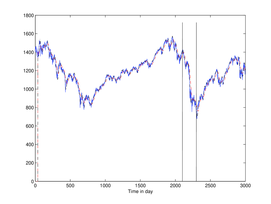
Figure 1: S&P 500 value (blue, –), its moving average (red, - -) and the proposed trend (black, .-)

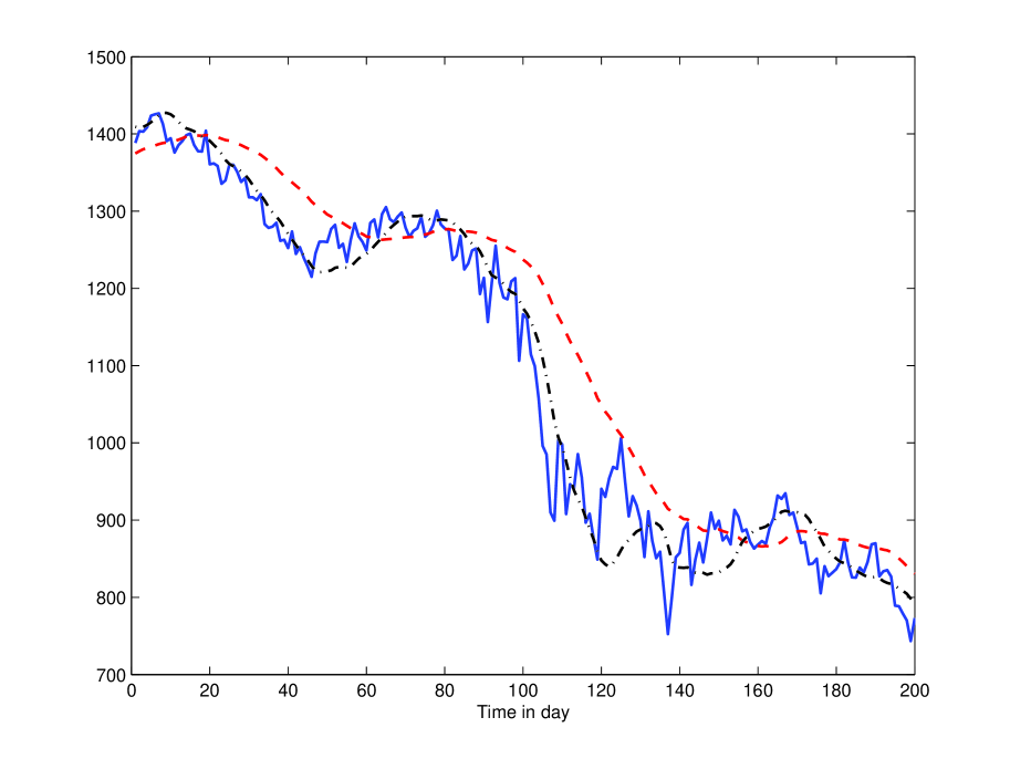
Figure 2: Zoom of Figure 1

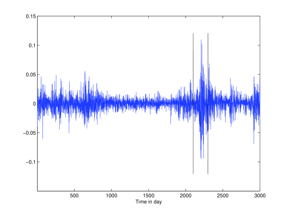
Figure 3: Log return

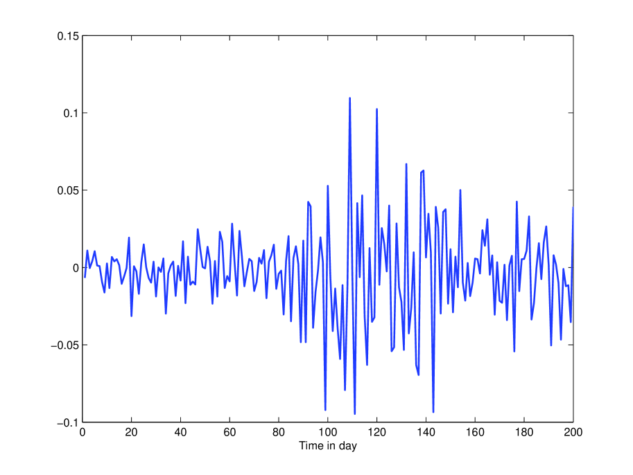
Figure 4: Zoom of Figure 3

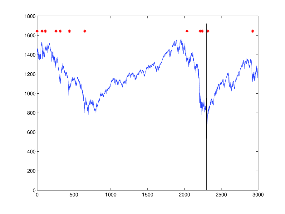
Figure 5: Abrupt change detection (red,$*$) on S&P 500

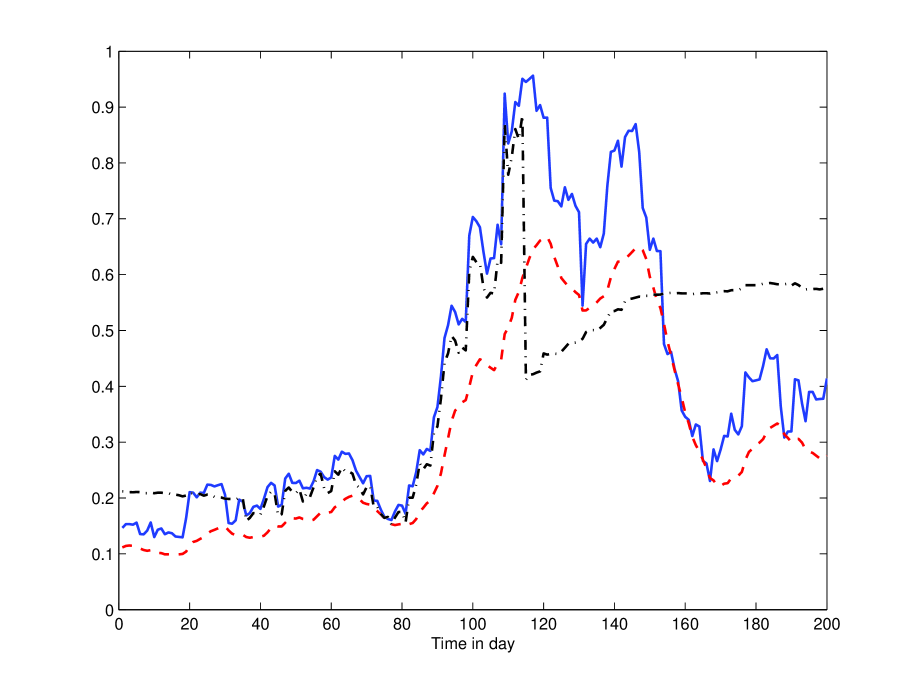
Figure 6: Usual volatility (blue, –), filtered volatility (red, - -), and time-scaled volatility (black, . -)

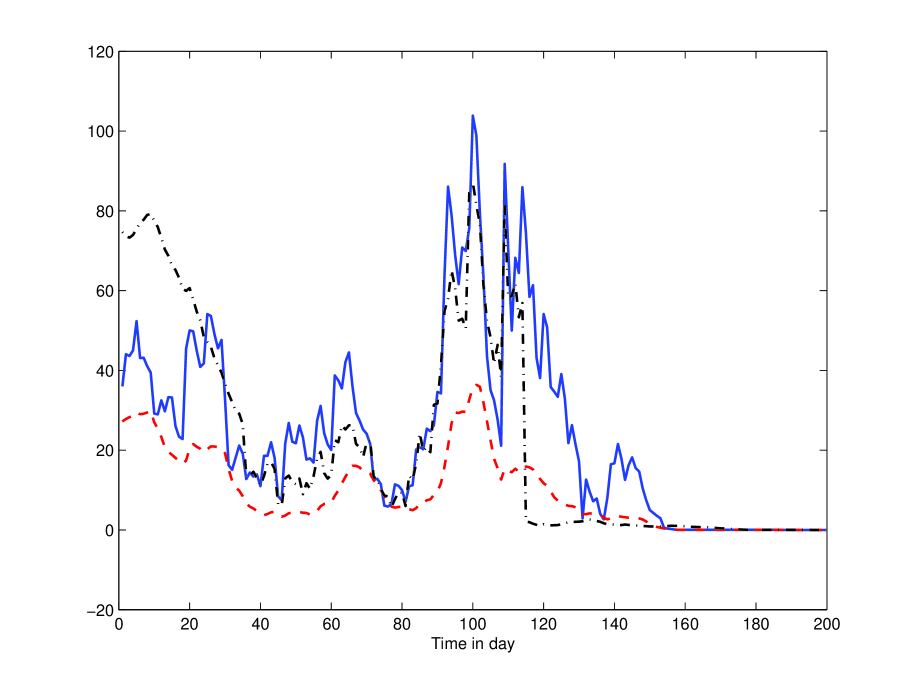
Figure 7: Call (blue, –), call with filtered volatility (red, - -) and call with time-scaled volatility (black, . -)

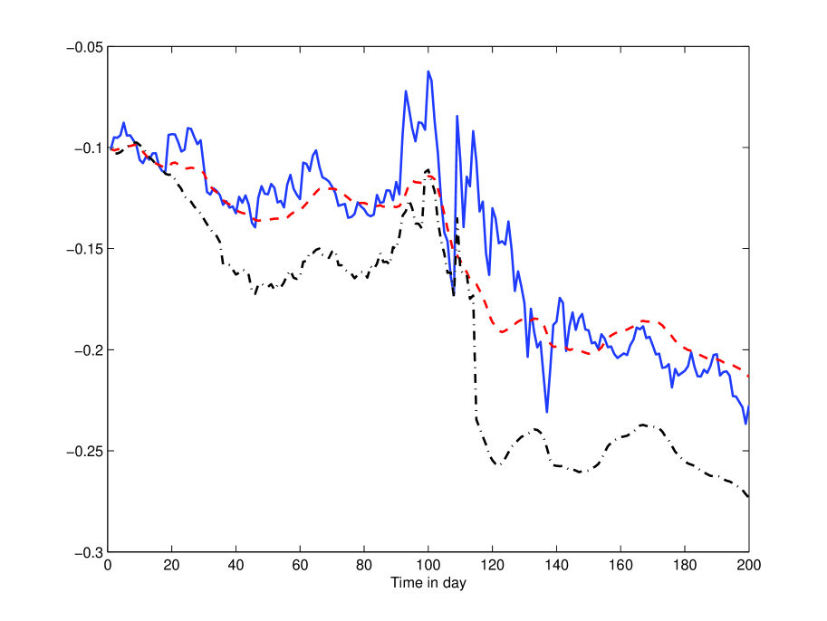
Figure 8: Hedging (blue, –), hedging with filtered volatility (red, - -), and hedging with time-scaled volatility (black, . -)

VII Conclusion

If further studies confirm our viewpoint on option pricing and dynamic hedging, it will open radically different roads which should bypass some of the most important difficulties encountered with today’s approaches. Let us emphasize as above and once again ([19, 22]) that a consequence of our setting might the obsolescence of the need of complex stochastic processes for modeling the underlying’s behavior. Taking into account

• the trends, which carry the information about jumps and other “violent” behaviors,

• their forecasting,

• not only the variance around the trend but also the skewness and the kurtosis,

should lead to new option pricing formulas, where the (geometric) Brownian motion will loose its preeminence.

American and other exotic options will be considered elsewhere.

References

- [1] L. Bachelier, “Théorie de la spéculation,” Ann. Sci. Éc. Norm. Sup., 3e série, vol. 17, pp. 21–86, 1900. English translation: “Theory of speculation,” in P. Cootner (Ed.): The Random Character of Stock Market Prices, pp. 17–78, MIT Press, 1964.
- [2] E.N. Barron, R. Jensen, “A stochastic control approach to the pricing of options,” Math. Operations Research, vol. 15, pp. 49–79, 1990.
- [3] T. Béchu, E. Bertrand, J. Nebenzahl, L’analyse technique ( éd.), Economica, 2008.
- [4] P. Bernhard, N. Farouq, S. Thiery, “Robust control approach to option pricing: a representation theorem and fast algorithm,” SIAM J. Control Optimiz., vol. 46, pp. 2280–2302, 2007.
- [5] F. Black, “Noise,” J. Finance, vol. 41, pp. 529–543, 1986
- [6] F. Black, “How we came up with the option formula,” J. Portfolio Management, vol. 15, pp. 4–8, 1989.
- [7] F. Black, M. Scholes, “The pricing of options and corporate liabilities,” J. Political Economy, vol. 81, pp. 637–654, 1973.
- [8] A.J. Boness, “Elements of a theory of stock-option values,” J. Political Economy, vol. 72, pp. 163–175, 1964.
- [9] F. Bronzin, Theorie der Prämiengeschäfte, Franz Deticke Verlag, 1908. Reprint: in W. Hafner, H. Zimmerman (Eds): Vinzenz Bronzin’s Option Pricing Models, pp. 23–111, Springer, 2009. English translation: “Theory of Premium Contracts,” in W. Hafner, H. Zimmerman (Eds): Vinzenz Bronzin’s Option Pricing Models, pp. 113–200, Springer, 2009.
- [10] R. Caldentey, M. Haugh, “Optimal control and hedging of operations in the presence of financial markets,” Math. Operations Research, vol. 31, pp. 285–304, 2006.
- [11] P. Cartier, Y. Perrin, “Integration over finite sets,” in F. & M. Diener (Eds): Nonstandard Analysis in Practice, pp. 195–204, Springer, 1995.
- [12] P. Chauveau, Évaluation par arbitrage des actifs financiers, Hermes – Lavoisier, 2010.
- [13] R.-A. Dana, M. Jeanblanc, Marchés financiers en temps continu, Economica, 1998. English translation: Financial Markets in Continuous Time, Springer, 2003.
- [14] M.H.A. Davis, V.G. Panas, T. Zariphopoulou, “European option pricing with transaction costs,” SIAM J. Control Optimiz., vol. 31, pp. 470–493, 1993.
- [15] E. Derman, N.N. Taleb, “The illusions of dynamic replication,” Quantit. Finance, vol. 5, pp. 323–326, 2005.
- [16] N. El Karoui, E. Gobet, Les outils stochastiques des marchés financiers, Éditions École Polytechnique, 2011.
- [17] M. Fliess, “Analyse non standard du bruit,” C.R. Acad. Sci. Paris Ser. I, vol. 342, pp. 797–802, 2006.
-
[18]
M. Fliess, C. Join, “Commande sans modèle et commande à modèle
restreint,” e-STA, vol. 5 (n∘ 4), pp. 1–23, 2008.
Available at:
http://hal.archives-ouvertes.fr/inria-00288107/en/ -
[19]
M. Fliess, C. Join, “A mathematical proof of the existence of
trends in financial time series,” in A. El Jai, L. Afifi, E. Zerrik
(Eds): Systems Theory: Modeling, Analysis and Control, pp.
43–62, Presses Universitaires de Perpignan, 2009. Available at:
http://hal.archives-ouvertes.fr/inria-00352834/en/ -
[20]
M. Fliess, C. Join, “Delta hedging in financial engineering:
towards a model-free setting,” in 18th Medit, Conf.
Control Automat., Marrakech, 2010. Available at:
http://hal.archives-ouvertes.fr/inria-00479824/en/ -
[21]
M. Fliess, C. Join, F. Hatt, “Volatility made observable at last,”
in 3es Journées Identif. Modélisation Expérimentale,
Douai, 2011. Available at:
http://hal.archives-ouvertes.fr/hal-00562488/ -
[22]
M. Fliess, C. Join, F. Hatt, “A-t-on vraiment besoin d’une approche
probabiliste en ingénierie financière?,” in Conf. Médit.
Ingénierie Sûre Systèmes Complexes, Agadir, 2011. Available at:
http://hal.archives-ouvertes.fr/hal-00585152/en/ - [23] M. Fliess, C. Join, M. Mboup, “Algebraic change-point detection,” Applicable Algebra Engin. Communic. Comput., vol. 21, pp. 131–143, 2010.
-
[24]
M. Fliess, C. Join, S. Riachy, “Rien de plus utile qu’une bonne
théorie: la commande sans modèle,” in JN-JD-MACS,
Marseille, 2011. Available at:
http://hal.archives-ouvertes.fr/hal-00581109/en/ -
[25]
M. Fliess, C. Join, H. Sira-Ramírez, “Non-linear estimation is
easy,” Int. J. Model. Identif. Control, vol. 4, pp.
12–27, 2008. Available at:
http://hal.archives-ouvertes.fr/inria-00158855/en/ - [26] J. Franke, W.K. Härdle, C.M. Hafner, Statistics of Financial Markets (3rd ed.). Springer, 2011.
- [27] N. Gradojevic, R. Gencay D. Kukolj, “Option pricing with modular neural networks,” IEEE Trans. Neural Networks, vol. 20, pp. 626-637, 2009.
- [28] E.G. Haug, “The history of option pricing and hedging,” in W. Hafner, H. Zimmerman (Eds): Vinzenz Bronzin’s Option Pricing Models, pp. 471–486, Springer, 2009.
- [29] E.G. Haug, N.N. Taleb, “Option traders use (very) sophisticated heuristics, never the Black-Scholes-Merton formula,” J. Econom. Behavior Organiz., vol. 77, pp. 97–106, 2011.
- [30] J.C. Hull, Options, Futures, and Other Derivatives (7th ed.), Prentice Hall, 2008.
- [31] J.M. Hutchinson, A.W. Lo, T. Poggio, “A nonparametric approach to pricing and hedging derivative securities via learning networks,” J. Finance, vol. 59, pp. 851–889, 1994.
- [32] C.D. Kirkpatrick, J.R. Dahlquist, Technical Analysis: The Complete Resource for Financial Market Technicians (2nd ed.), FT Press, 2010.
- [33] A. Krouglov, “Intuitive proof of Black-Scholes formula based on arbitrage and properties of lognormal distribution,” Manuscript, 2006. Available at http://arxiv.org/abs/physics/0612022
- [34] D. Lamberton, B. Lapeyre, Introduction au calcul stochastique appliqué à la finance (3e éd.), Ellipses, 2012. English translation: Introduction to Stochastic Calculus Applied to Finance, Chapman & Hall, 1996.
- [35] D. MacKenzie, “Constructing a market, performing theory: The historical sociology of a financial derivatives exchange,” Amer. J. Sociology, vol. 103, pp. 107–145, 2003.
- [36] M. Mboup, C. Joinn M. Fliess, “Numerical differentiation with annihilators in noisy environment,” Numer. Algor., vol. 50, pp. 439–467, 2009.
- [37] W.M. McEneaney, “A robust control framework for option pricing,” Math. Operations Research, vol. 22, pp. 202–221, 1997.
- [38] P. Mehrling, Fischer Black and the Revolutionary Idea of Finance, Wiley, 1985.
- [39] R.C. Merton, “Theory of rational option pricing,” Bell. J. Economics Management, vol. 4, pp. 141–183, 1973.
- [40] R.C. Merton, “Option pricing when underlying stock returns are discontinuous,” J. Financial Economics, vol. 3, pp. 125–144, 1976.
- [41] H. Pham, Optimisation et contrôle stochastique appliqués à la finance, Springer, 2007. English translation: Continuous-time Stochastic Control and Optimization with Financial Applications, Springer, 2009.
- [42] R. Portet, P. Poncet, Finance de marché (3e éd.), Dalloz, 2012.
- [43] J.A. Primbs, “Dynamic hedging of basket options under proportional transaction costs using receding horizon control,” Int. J. Control, vol. 82, pp. 1841–1855, 2009.
- [44] P.A. Samuelson, “Rational theory of warrant pricing,” Indust. Manag. Rev., vol. 6, pp. 13–31, 1965.
- [45] P.A. Samuelson, R.C. Merton, “A complete model of asset prices that maximizes utility,” Ind. Manag. Rev., vol. 10, pp. 17–46, 1969.
- [46] W. Schachermayer, J. Teichmann, “How close are the option pricing formulas of Bachelier and Black-Merton-Scholes?,” Math. Finance, vol. 18, pp. 55–76, 2008.
- [47] C.W. Smith Jr., “Option pricing,” J. Financial Economics, vol. 3, pp. 3–51, 1976.
- [48] C. Sprenkle, “Warrant prices as indicators of expectations and performances,” Yale Economic Essays I, pp. 178–231, 1961.
- [49] A. Vollert, A Stochastic Control Framework for Real Options in Strategic Valuation, Birkhäuser, 2003.
- [50] P. Wilmott, Paul Wilmott on Quantitative Finance, 3 vol. (2nd ed.), Wiley, 2006.
- [51] H. Zimmermann, “A review and evaluation of Bronzin’s contribution from a financial economics perspective,” in W. Hafner, H. Zimmerman (Eds): Vinzenz Bronzin’s Option Pricing Models, pp. 207–291, Springer, 2009.