Pattern formation by kicked solitons in the two-dimensional Ginzburg-Landau medium with a transverse grating

Abstract

We consider the kick (tilt)-induced mobility of two-dimensional (2D) fundamental dissipative solitons in models of bulk lasing media based on the 2D complex Ginzburg-Landau (CGL) equation including a spatially periodic potential (transverse grating). The depinning threshold, which depends on the orientation of the kick, is identified by means of systematic simulations, and estimated by means of an analytical approximation. Various pattern-formation scenarios are found above the threshold. Most typically, the soliton, hopping between potential cells, leaves arrayed patterns of different sizes in its wake. In the single-pass-amplifier setup, this effect may be used as a mechanism for the selective pattern formation controlled by the tilt of the input beam. Freely moving solitons feature two distinct values of the established velocity. Elastic and inelastic collisions between free solitons and pinned arrayed patterns are studied too.

I Introduction

A well-known fact is that the formation of stable dissipative solitons—most typically, in lasing media Rosa ; lasers and plasmonic cavities plasmonics —relies upon the simultaneous balance of competing conservative and dissipative effects in the system, i.e., respectively, the diffraction and self-focusing nonlinearity, and linear and nonlinear loss and gain DS . The generic model describing media where stable dissipative solitons emerge via this mechanism is based on the complex Ginzburg-Landau (CGL) equations with the cubic-quintic (CQ) combination of gain and loss terms, which act on top of the linear loss lasers . In addition to modeling the laser-physics and plasmonic settings, the CGL equations, including their CQ variety, serve as relevant models in many other areas, well-known examples being Bose-Einstein condensates in open systems (such as condensates of quasi-particles in solid-state media) BEC , reaction-diffusion systems MCCROSS , and superconductivity supercond . Thus, the CGL equations constitute a class of universal models for the description of nonlinear waves and pattern formation in dissipative media AK .

The CGL equation with the CQ nonlinearity was originally postulated by Petviashvili and Sergeev Petv as a model admitting stable localized two-dimensional (2D) patterns. Subsequently, systems of this type were derived or introduced phenomenologically in many physical settings, and a great deal of 1D and 2D localized solutions, i.e., dissipative solitons, have been studied in detail in them Boris -Vladimir .

A 2D model of laser cavities with an internal transverse grating, based on the CQ-CGL equation supplemented by a spatially periodic (lattice) potential, which represents the grating, was introduced in Ref. leblond1 . Note that the currently available laser-writing technology makes it possible to fabricate permanent gratings in bulk media Jena . In addition, in photorefractive crystals virtual photonic lattices may be induced by pairs of pump laser beams with the ordinary polarization, which illuminate the sample in the directions of $x$ and $y$, while the probe beam with the extraordinary polarization is launched along axis $z$ Moti-general . In fact, the laser cavity equipped with the grating may be considered as a photonic crystal built in the active medium. Periodic potentials are also known in passive optical systems, driven by external laser beams and operating in the temporal domain, unlike the spatial-domain dynamics of the active systems. In such systems, effective lattices may be induced by spatial modulation of the pump beam Firth ; advances .

A notable fact reported in Ref. leblond1 is that localized vortices, built as sets of four peaks pinned to the periodic potential, may be stable without the presence of the diffusion term in the CGL laser model,which is necessary for the stabilization of dissipative vortex solitons in uniform media, see, e.g., Ref. Mihalache , but is unphysical for waveguiding models (the diffusion term is relevant in models describing light trapped in a cavity, where the evolutional variable is time, rather than the propagation distance Fedorov ). In subsequent works, stable fundamental and vortical solitons in 2D trapping_potentials_2D and 3D trapping_potentials_3D CGL models with trapping potentials were studied in detail. Spatiotemporal dissipative solitons in the CQ-CGL model of 3D laser cavities including the transverse grating were investigated too trapping_potentials_3D . Both fundamental and vortical solitons were found in a numerical form as attractors in the latter model, and their stability against strong random perturbations was tested by direct simulations.

While the stability of various 2D localized patterns has been studied thoroughly in the framework of the CQ-CGL equations with the transverse lattice potential used as the stabilizing factor, a challenging problem is mobility of such 2D dissipative solitons under the action of a kick applied across the underlying lattice.

Actually, the action of the kick in this context implies the application of a tilt to the beam. It should be noted that the CGL equation models single-pass optical amplifiers, as well as laser cavities. In the latter case the evolution is considered in the temporal domain, while in the former the evolution variable is the propagation distance. In order to build the required initial data in a laser cavity, the tilt should be applied very quickly. This may be achieved by means of an optically induced grating or mirrors, using some fast device. On the other hand, in the single-pass amplifier the input is an incident beam, the tilt being a mere misalignment between the beam and the amplifier’s axis. Below, we present the analysis in terms of the amplifier’s setup, which is more straightforward for the experimental implementation.

Thus, we assume that an external source produces a beam, which is shaped into the fundamental-soliton mode of the amplifier by means of an adequate setup. Then, the direction of this input beam is slightly tilted with respect to the amplifier’s axis, allowing the transverse part of the beam’s momentum to acts as the kick applied to the fundamental spatial soliton.

Furthermore, we demonstrate that the effective hopping motion of the kicked soliton through cells of the periodic potential can be used for controlled creation of various patterns filling these cells (or a part of them).

Thus, the main objective of this work is to study the mobility of the 2D fundamental solitons, and scenarios of the pattern formation by kicked ones, in the framework of the CQ-CGL models with the lattice potential. The model is formulated in Section II, which also presents an analytical approximation, that, using the concept of the Peierls-Nabarro (PN) barrier, makes it possible to predict, with a reasonable accuracy, the minimum (threshold) strength of the kick necessary for depinning of the quiescent soliton trapped by the lattice. The main numerical results for the mobility of the kicked soliton, and various scenarios of the pattern creation in the wake of the soliton hopping between cells of the potential lattice, are reported in Section III, while Section IV deals with collisions between a freely moving soliton and a standing structure created and left by it, in the case of periodic boundary conditions (which correspond to a pipe-shaped amplifier, i.e., one in the form of a hollow cylinder). In particular, elastic collisions provide for an example of a soliton Newton’s cradle. The paper is concluded by Section V.

II The model and analytical approximations

II.1 The Ginzburg-Landau equation

Following Refs. leblond1 and trapping_potentials_2D , the scaled CQ-CGL equation for the evolution of the amplitude of the electromagnetic field, $u(X,Y,Z)$, in two dimensions with transverse coordinates $\mathbf{R}=(X,Y)$, along the propagation direction, $Z$, is written as

$$\frac{\partial u}{\partial Z}=\left[-\delta+iV(X,Y)+\frac{i}{2}\nabla_{\perp}^{2}+(i+\epsilon)|u|^{2}-(i\nu+\mu)|u|^{4}\right]u,$$ (1)

where the paraxial diffraction is represented by $\nabla_{\perp}^{2}=\partial^{2}/\partial X^{2}+\partial^{2}/\partial Y^{2}$ , real coefficients $\delta$, $\epsilon$, and $\mu$ account for the linear loss, cubic gain, and quintic loss, respectively, and coefficient $\nu>0$ accounts for the saturation of the Kerr nonlinearity. The transverse grating is represented by the periodic potential,

$$V(X,Y)=-V_{0}\left[\cos(2X)+\cos(2Y)\right],$$ (2)

of depth $2V_{0}$, with the period scaled to be $\pi$. Localized modes produced by Eq. (1), which physically correspond to light beams self-trapped in the $\left(X,Y\right)$ plane, are characterized by the total power,

$$P=\int\int|u(X,Y,Z)|^{2}dXdY.$$ (3)

In the simulations, Eq. (1) was solved by means of the standard fourth-order Runge-Kutta scheme in the $Z$-direction, and five-point finite-difference approximation for the transverse Laplacian. As specified below, we used periodic boundary conditions. The integration domain correspond to an $(X,Y)$ matrix of $256\times 256$ grid points covering the area of $\left|X\right|,\left|Y\right|\leq 22$. Generic results for the mobility of fundamental dissipative solitons can be adequately represented by fixing the following set of parameters:

$$\delta=0.4,\epsilon=1.85,\mu=1,\nu=0.1,V_{0}=1,$$ (4)

for which the quiescent fundamental soliton is stable.

II.2 The description of tilted beams

In simulations of Eq. (1), the kick (i.e., tilt) was applied to the self-trapped beam, as usual, by multiplying the respective steady state, $u_{0}$, by $\exp\left(i\mathbf{k}_{0}\mathbf{R}\right)$, with the vectorial strength of the kick defined as

$$\mathbf{k}_{0}=\left(k_{0}\cos\theta,k_{0}\sin\theta\right),$$ (5)

where the square-lattice symmetry of potential (2) makes it sufficient to confine the orientation angle, $\theta$, to interval $0\leq\theta\leq\pi/4$. In terms of the amplifier setup, a small angle $\varphi$ between the carrier wave vector $\mathbf{K}_{0}=(K_{x},K_{y},K_{z})$ of the beam (in physical units) and the $Z$-axis, gives rise to the transverse component $\mathbf{k}_{0}$ which corresponds to the kick. The paraxial approximation implies that

$$\varphi\approx\sqrt{K_{x}^{2}+K_{y}^{2}}/K_{z}~{}\ll 1,$$ (6)

Before studying effects induced by the kick, it is relevant to explain the corresponding physical setting in more detail, making it sure that the tilted beams remain within the confines of the paraxial description.

Equation (1) can be derived from the underlying wave equation by means of the standard slowly varying envelope approximation (SVEA) Rosa . For this purpose, electric field $E$ (in its scalar form) is split into a slowly varying amplitude and the rapidly oscillating carrier either as

$$E=\mathcal{A}(x,y,z-vt)e^{i\left(K_{x}x+K_{y}y+K_{z}z-\omega t\right)}+\mathrm{c.c.},$$ (7)

where $(x,y,z,t)$ are the coordinates and time in physical units, $v$ is the group velocity, and $\mathrm{c.c.}$ stands the complex conjugate, or, alternatively, as

$$E=A(x,y,z-vt)e^{i\left(K_{z}z-\omega t\right)}+\mathrm{c.c.}$$ (8)

The difference is that that carrier wave is oblique in Eq. (7), while in Eq. (8) it is always defined as the straight one. Obviously, $A(x,y,z-vt)=\mathcal{A}(x,y,z-vt)e^{i\left(K_{x}x+K_{y}y\right)}$, and the two forms are fully equivalent within the framework of the SVEA if the oscillations due to the term $e^{i\left(K_{x}x+K_{y}y\right)}$ are not essentially faster than the transverse variations of the beam described by amplitude $\mathcal{A}(x,y,z-vt)$. Thus, the SVEA can be fixed in the form of Eq. (8), with $K_{z}=2\pi n/\lambda$, where $n$ the linear index of the medium.

Further, to proceed to normalized equation (1), we set $\left\{X,Y\right\}\equiv w^{-1}\left\{x,y\right\}$, where $w$ is a characteristic scale of the beam’s width—say, $w\sim 10$ $\mathrm{\mu}$m for narrow beams, if the underlying wavelength (in vacuum) is $\lambda\sim 1$ $\mathrm{\mu}$m. Accordingly, the period of grating (2) is $\pi w$ in the physical units. Note that $w\sim 10$ $\mathrm{\mu}$m corresponds to the period $\pi w\sim 30$ $\mathrm{\mu}$m, which is relevant estimate (gratings with the period on this order of magnitude can be readily manufactured). Then, the scaled propagation distance is $Z=z/(K_{z}w)\equiv\left(\lambda/2\pi nw\right)z$, and the scale wave amplitude is

$$u=\sqrt{\frac{1}{2}\mathrm{Re}\left(\chi^{(3)}\right)}\frac{\omega w}{c}A,$$

where $\chi^{(3)}$ is the third-order nonlinear susceptibility. Further, the respective rescaling of the wave vector components is given by $\left\{k_{x},k_{y}\right\}=w\left\{K_{x},K_{y}\right\}$. Thus, the deviation angle can be estimated as $\tan\varphi=\sqrt{K_{x}^{2}+K_{y}^{2}}/K_{z}\equiv\left(\lambda/2\pi nw\right)\sqrt{k_{x}^{2}+k_{y}^{2}}$, and, for generic tilted modes, with $\sqrt{k_{x}^{2}+k_{y}^{2}}\sim 1$ in the scaled notation, condition (6) for the validity of the paraxial approximation amounts to $\lambda\ll 2\pi nw$, which is nothing but the standard paraxial assumption.

With the above-mentioned typical values, $\lambda\sim 1$ $\mathrm{\mu}$m and $w\sim 10$ $\mathrm{\mu}$m, along with $n\approx 1.5$, the above estimate yields $\varphi\sim 0.01$ (in radians). Then, the minimum propagation distance relevant to the experiment, $z\sim 1$ cm, corresponds to the transverse deviation of the tilted beam $\Delta x\sim 100$ $\mathrm{\mu}$m, which can be easily detected and employed in applications.

II.3 Analytical estimates

The first characteristic of kink-induced effects is the threshold value, $\left(k_{0}\right)_{\mathrm{thr}}$, such that the soliton remains pinned at $k_{0}<\left(k_{0}\right)_{\mathrm{thr}}$ and escapes at $k_{0}>\left(k_{0}\right)_{\mathrm{thr}}$.To develop an analytical approximation which aims to predict the threshold, one can, at the lowest order, drop the loss and gain terms, as well as the lattice potential, in Eq. (1). The corresponding 2D nonlinear Schrödinger equation gives rise to the commonly known family of Townes soliton, which share a single value of the total power, $P_{\mathrm{T}}\approx 5.85$ Berge' . The family may be approximated by the isotropic Gaussian ansatz with arbitrary amplitude $A$,

$$u\left(Z,R\equiv\sqrt{X^{2}+Y^{2}}\right)=A\exp\left(ibZ-\frac{\pi A^{2}}{2P_{\mathrm{T}}}R^{2}\right),$$ (9)

and propagation constant $b=A^{2}/4$ Anderson . Then, taking into regard the loss and gain terms as perturbations, one can predict the equilibrium value of the amplitude from the power-balance equation,

$$\delta\cdot P+\mu\int\int\left|u\left(X,Y\right)\right|^{6}dXdY=\epsilon\int\int\left|u\left(X,Y\right)\right|^{4}dXdY.$$ (10)

The substitution of approximation (9) into Eq. (10) leads to a quadratic equation for $A^{2}$, with roots

$$A^{2}=\frac{3\epsilon\pm\sqrt{3\left(3\epsilon^{2}-16\mu\delta\right)}}{4\mu},$$ (11)

the larger one corresponding to a stable dissipative soliton (cf. a similar analysis for the CQ-CGL model in 1D PhysicaD ).

Proceeding to the kicked soliton, the threshold magnitude of the kick for the depinning, $\left(k_{0}\right)_{\mathrm{thr}}$, can be estimated from the comparison of the PN potential barrier, $U_{\mathrm{PN}}$, and the kinetic energy of the kicked soliton, $E_{\mathrm{kin}}$. The Galilean invariance of Eq. (1) HS (in the absence of the lattice potential) implies that kick (5) gives rise to “velocity” $\mathbf{k}_{0}$, so that the solution will become a function of $\mathbf{R}-\mathbf{k}_{0}Z\equiv\mathbf{R-}\mathbf{\Upsilon}$, instead of $\mathbf{R}$, the corresponding kinetic energy being

$$E_{\mathrm{kin}}=(1/2)Pk_{0}^{2}$$ (12)

($P$ plays the role of the effective mass of the soliton). Further, assuming that the kicked soliton moves in the direction of $\theta$ [see Eq. (5)], the effective energy of the interaction of the soliton, taken as per approximation (9), with lattice potential (2), treated as another perturbation, is

$$E_{\mathrm{pot}}(\Upsilon) = -V_{0}\int\int\left[\cos(2X)+\cos(2Y)\right]\left|u\left(X-\Upsilon\cos\theta,Y-\Upsilon\sin\theta\right)\right|^{2}dXdY$$ (13)

$$= -V_{0}P\exp\left(-\frac{P_{\mathrm{T}}}{\pi A^{2}}\right)\left[\cos\left(2\Upsilon\cos\theta\right)+\cos\left(2\Upsilon\sin\theta\right)\right],$$

where $\Upsilon$ is the shift of the soliton from $X=Y=0$ in the direction of $\theta$. As follows from this expression, the PN barrier, i.e., the difference between the largest and smallest values of the potential energy, is estimated as

$$E_{\mathrm{PN}}=V_{0}P\exp\left(-\frac{P_{\mathrm{T}}}{\pi A^{2}}\right)\Delta(\theta),$$ (14)

where $\Delta(\theta)$ is the difference between the maximum and minimum of function $\cos\left(2\Upsilon\cos\theta\right)+\cos\left(2\Upsilon\sin\theta\right)$. Obviously, $\Delta(0)=2$ and $\Delta\left(\pi/4\right)=4$. For intermediate values of $\theta$, it may be approximated by the difference of the values of the function between points $\Upsilon=0$ and $\Upsilon=\pi/\left(2\cos\theta\right)$, i.e.,

$$\Delta(\theta)\approx 3-\cos\left(\pi\tan\theta\right).$$ (15)

Finally, the threshold value of the kick is determined by the depinning condition, $E_{\mathrm{kin}}=E_{\mathrm{PN}}$, i.e.,

$$\left(k_{0}\right)_{\mathrm{thr}}=\sqrt{2V_{0}\left[3-\cos\left(\pi\tan\theta\right)\right]}\exp\left(-\frac{P_{\mathrm{T}}}{2\pi A^{2}}\right).$$ (16)

This prediction is compared with numerical results below.

III Numerical results: The mobility and pattern formation

The stable fundamental soliton constructed in the model based on Eqs. (1) and (2) at parameter values (4) is shown in Fig. 1. For these parameters, analytical prediction (11) yields the amplitude of the stable soliton $A\approx$ $\allowbreak 1.496\,$, which is quite close to the amplitude of the numerically found solution in Fig. 1: $A\approx$ $\allowbreak 1.479\,$, which implies that the isotropic Gaussian (9) is quite appropriate as the ansatz for the description of static properties of the solitons.

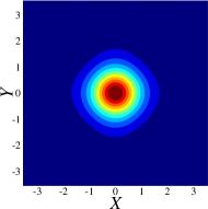
(a) Amplitude

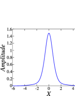
(b) Profile

Figure 1: (Color online) The stable fundamental soliton: (a) the contour plot of the local amplitude, $|u\left(X,Y\right)|$; (b) the cross-section profile of $|u(X)|$ at $Y=0$. The soliton emphasizes the potential : $V(X,Y)=-\left[\cos\left(2X\right)+\sin\left(2X\right)\right]$

III.1 The formation of arrayed soliton patterns

First we consider the solitons kicked with $\theta=0$, i.e., along bonds of the lattice, see Eq. (5). Below the threshold value of the kick’s strength, whose numerically found value is

$$\left(k_{0}\right)_{\mathrm{thr}}(\theta=0)\approx 1.6865,$$ (17)

the kicked soliton exhibits damped oscillations, remaining trapped near a local minimum of the lattice potential, as shown in Fig. 2. Originally (at $0<z<8$ in Fig. 2), the total power (3) increases, and then it drops to the initial value, $P\approx 3.2$. As a result of the kick, a portion of the wave field passes the potential barrier and penetrates into the adjacent lattice cell, but, at $k_{0}<\left(k_{0}\right)_{\mathrm{thr}}$, the power carried by the penetrating field is not sufficient to create a new soliton, and is eventually absorbed by the medium.

On the other hand, analytical prediction (16) yields $\left(k_{0}\right)_{\mathrm{thr}}(\theta=0)\approx 1.32$. A relative discrepancy $\simeq 20\%$ with numerical value (17) is explained by the fact that, near the depinning threshold, the moving soliton suffers appreciable deformation, while the analytical approach assumed the fixed shape (9), and it did not take into account energy losses (the latter factor makes the actual threshold somewhat higher). In other cases considered below, see Eqs. (18) and (19), the analytical predictions for $\left(k_{0}\right)_{\mathrm{thr}}$ is also $\simeq 20\%$ smaller than their numerically found counterparts

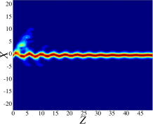
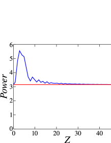
Figure 2: (Color online) (a): The evolution of the local amplitude, $|u(X,Z)|$, in the cross section, $Y=0$, of the fundamental soliton kicked with the under-threshold strength, $k_{0}=1.61$ at $\theta=0$. (b) The evolution of the total power in this case. The horizontal line designates the power of the quiescent fundamental soliton.

If the kick is sufficiently strong, $k_{0}>\left(k_{0}\right)_{\mathrm{thr}}$, the portion of the wave field passing the potential barrier has enough power to create a new dissipative soliton in the adjacent cell. The emerging secondary soliton may either stay in its cell, or keep moving through the lattice.

(a) $Z=2.65$

(b) $Z=4.70$

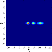
(c) $Z=8.51$

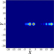
(d) $Z=14.00$

Figure 3: (Color online) The evolution of the local field amplitude, $|u(X,Y)|$, corresponding to the kicked soliton, for $k_{0}=1.6878$ and $\theta=0$. The field distributions are displayed at different values of propagation distance $Z$.

Figure 3 demonstrates the creation of two new solitons at $k_{0}=1.6878$, which slightly exceeds the threshold value (17). This figure represents a generic dynamical scenario, that can be summarized as follows:

• the initial soliton (or a part of it) passes the potential barrier and gets into the adjacent (second) cell;

• it then stays for some time in that cell;

• if the initial kick is not strong enough, the secondary soliton permanently stays at this location;

• if the kick is harder, the soliton again passes the potential barrier, getting into the third cell, and may continue to move through the grating;

• a portion of the wave field of the secondary soliton stays in the second cell and grows into a full soliton in this cell;

• if the kick is not sufficient to continue the filling of farther cells, oscillations of all the persistent solitons relax.

The present case is further illustrated in Fig. 4 by the plot for the evolution of the total power, which shows that $P$ attains the first maximum at $Z=15.89$, and then oscillates. Every minimum correspond to the collision between the two solitons. For the sake of comparison, four horizontal lines in the figure mark the powers corresponding to the single stable soliton ($P_{\mathrm{sol}}\approx 3.15$), multiplied, respectively, by $\ 1$, $2$, $3$, or $4$.

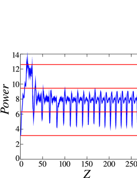
Figure 4: (Color online) The evolution of the total power of the pattern in the case displayed in Fig. 3, with $k_{0}=1.6878$ and $\theta=0$. The horizontal lines show the powers for the sets of 1, 2, 3 and 4 quiescent fundamental solitons.

It has been found that solitons can duplicate several times, thus forming extended patterns in the form of soliton arrays. The increase of the kick’s magnitude leads to the decrease of the number of the solitons forming this pattern, as the soliton moves faster and does not spend enough time in each cell to create a new soliton trapped in it. In particular, Fig. 5 demonstrates that only one additional soliton is generated at $k_{0}=1.6872$, both solitons remaining pinned (note that this value is smaller than $k_{0}=1.6878$ appertaining to Fig. 3). Further, at $k_{0}=2.082$ the soliton performs unhindered motion, without leaving any stable pattern in its wake (not shown here in detail).

(a) $Z=2.65$

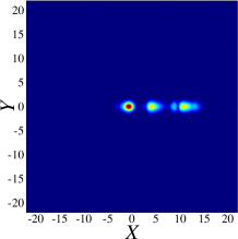
(b) $Z=8.51$

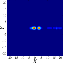
(c) $Z=13.28$

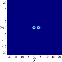
(d) $Z=21.43$

Figure 5: (Color online) The same as in Fig. 3, but for $k_{0}=1.6872$ and $\theta=0$.

On the other hand, the smaller kick can initiate the creation of an arrayed pattern. This outcome of the evolution is shown in Fig. 6, where the array of five solitons is created, starting with the soliton initially kicked by $k_{0}=1.694$, in addition to which a free soliton keeps moving as a quasi-particle (cf. Ref. Kominis ), until it collides with the array from the opposite direction, due to the periodic boundary conditions along $X$, and is subsequently absorbed by the array (the collision is displayed in panel 6(f), where an additional soliton is observed at $X<0$). This dynamical scenario is additionally illustrated below by Fig. 11.

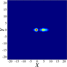
(a) $Z=2.63$

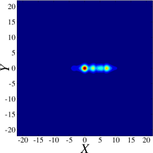
(b) $Z=4.68$

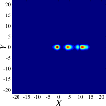
(c) $Z=8.48$

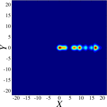
(d) $Z=12.05$

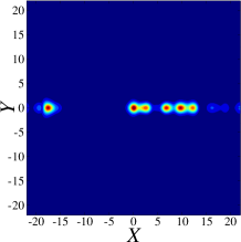
(e) $Z=17.67$

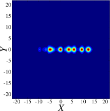
(f) $Z=24.12$

Figure 6: (Color online) The same as in Figs. 3 and 5, but for $k_{0}=1.694$. In this case, the kicked soliton eventually creates an arrayed set of five solitons (in panel (f), the additional freely moving (sixth) soliton hits the array from the opposite direction, completing its round trip in the system).

The emerging array remains in an excited state, featuring localized density waves running across it, as shown, on a much longer scale of $Z$, by means of the cross-section picture in Fig. 7). It is worthy to note that the wave is reflected from the last pinned soliton. Such localized density perturbations propagating through a chain of pinned solitons are similar to the so-called “ super-fluxons”, which were investigated experimentally and theoretically in arrays of fluxons (topological solitons, representing magnetic-flux quanta) pinned in a long Josephson junction with a periodic lattice of local defects super , as well as in an array of mutually repelling solitons forming a Newton’s cradle in a two-component model of binary Bose-Einstein condensates cradle .

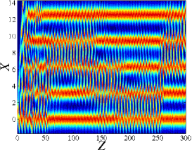
Figure 7: (Color online) Evolution of the local amplitude, $|u(X,Z)|$, in the cross-section plane, $Y=0$, in the same case as in Fig. 6 ($k_{0}=1.694$ and $\theta=0$).

III.2 The dependence of the outcome of the evolution on the strength of the initial kick

Results of the systematic analysis of the model are summarized in Fig. 8, where the number of solitons in the stable arrayed patterns established by the end of the simulation, is plotted versus the initial kick $k_{0}$ for $\theta=0$,where intervals of the values of $k_{0}$ corresponding to constant numbers of the solitons are adduced.

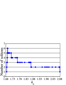
Figure 8: (Color online)The number of solitons in the established pattern versus the kick’s strength, $k_{0}$, at $\theta=0$. In narrow gaps between intervals presented in the graphic, the number cannot be defined exactly, as it changes there by $1$

In case the free soliton collides with the quiescent array after performing the round trip in the system with the periodic boundary conditions, see the example above in Fig. 6, and an additional one (for four solitons) in Figs. 9 and 10, the number of solitons was counted just before the first such collision. Otherwise, the number was recorded after any motion in the system would cease.

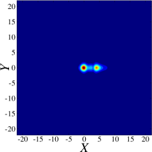
(a) $Z=2.60$

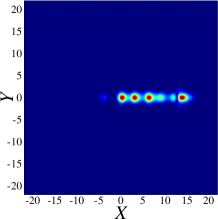
(b) $Z=12.47$

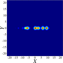
(c) $Z=23.09$

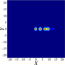
(d) $Z=299.68$

Figure 9: (Color online) The same as in Fig. 6, but for $k_{0}=1.705$. In this case, a free soliton splits away from the quiescent array, then hits it from the other side, and gets absorbed by it.

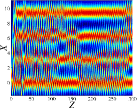
Figure 10: (Color online) The top view of the same dynamical picture as in Fig. 9.

The results demonstrate that the number of solitons in the established patterns rapidly increases from 1 at $k_{0}\leq(k_{0})_{\mathrm{thr}}\approx 1.6865$ [see Eq. (17)] to a maximum of five solitons, plus a sixth freely moving one, at $k_{0}=1.6927$. New solitons add to the established pattern according to the scenario outlined by means of the bullet items in the previous subsection. At $k_{0}>1.6927$, the soliton number decreases by steps with an increasing length of the corresponding intervals of the kick’s strength, see Fig. 8.

As mentioned above, the largest number of six solitons is attained at $1.6927<k_{0}<1.6942$. In addition to Figs. 6 and 7, this situation is illustrated by Fig. 11), where the averaged total power is $P=23$, see panel 11(b). The horizontal reference lines in this figure show the power levels corresponding to a single quiescent soliton (recall $P_{\mathrm{sol}}\approx 3.15$), multiplied by factors from $1$ to $7$, which demonstrates that the total power of the six-soliton complex exceeds the seven-fold power of the single soliton. This is due to the fact that the energy of the moving soliton is roughly twice that of a soliton at rest.

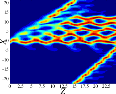
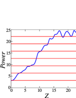
Figure 11: (Color online) (a): The field amplitude, $\left|u\left(X,Z\right)\right|$, in the cross section $Y=0$, and (b) the evolution of the total power, for the kick’s strength $k_{0}=1.693$ at $\theta=0$, which leads to the establishment of the six-soliton pattern.

At $k_{0}\geq 2.082$, the kicked soliton moves freely across the simulation domain, see Fig. 12. In this case, the figure demonstrates that the soliton’s velocity increases, approaching a certain limit value. The computation of the velocity was performed by means of the Lagrange’s interpolation of the numerical data to accurately identify the soliton’s center. To display the results, small-scale oscillations of the velocity of the soliton passing the periodic potential (obviously, the velocity is largest and smallest when the solitons traverses the bottom and top points of the potential, respectively) have been smoothed down by averaging the dependence over about fifteen periods.

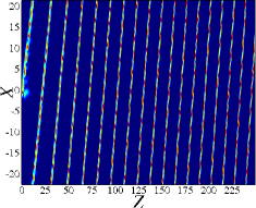
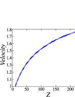
Figure 12: (Color online) (a) The distribution of the field amplitude, $\left|u\left(X,Z\right)\right|$ in cross section $Y=0$, and (b) the evolution of the velocity of the fundamental soliton kicked by $k_{0}=2.1$ at $\theta=0$.

III.3 The evolution initiated by an oblique kick

The application of the kick under an angle to the lattice, i.e., with $\theta\neq 0$ [see Eq. (5)], was considered too. The results are summarized in Table 1 for $\theta=\pi/4$ (the kick oriented along the diagonal), and, below, in Table 2 for $\theta=\pi/8$.

Number of solitons	Range of $k_{0}$
$1$	$k_{0}\in[0,2.355]$
$0$	$k_{0}\in[2.36,4.337]$
$1$	$k_{0}\in[4.563,10]$

Table 1: The number of solitons in the established pattern versus the kick’s strength, $k_{0}$, at $\theta=\pi/4$.

For $\theta=\pi/4$, the initial soliton remains pinned at

$$k_{0}\leq\left(k_{0}\right)_{\mathrm{thr}}\left(\theta=\pi/4\right)=2.166,$$ (18)

and it is destroyed at $2.25<k_{0}<4.337$. At $k_{0}>4.337$, the single soliton survives, moving freely along the diagonal direction. Thus, the final number of the solitons in this case is $1$ or $0$ (see Table 1), and no new solitons are generated. As concerns the comparison with the analytical prediction (16), it yields $\left(k_{0}\right)_{\mathrm{thr}}\left(\theta=\pi/4\right)\approx 1.87$, which, as well as in the case of $\theta=0$, is somewhat lower than its numerical counterpart.

The kick with much larger values of $k_{0}$ (one or two orders of magnitude higher than in Table 1) causes the generation of dark-soliton structures, supported by a nonzero background filling the entire domain (the total power may then exceed that of the single soliton by a factor $\sim 1000$). Inspection of Fig. 13 reveals stable holes in the continuous background, whose centers coincide with phase singularities (see Fig. 13). These holes represent vortices supported by the finite background.

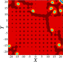
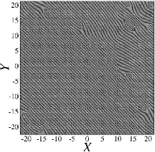
Figure 13: (Color online) The distribution of the field amplitude, $\left|u\left(X,Y\right)\right|$ (a) and phase (b) in the pattern produced by kicking the fundamental soliton in the diagonal direction ($\theta=\pi/4$) very hard, with $k_{0}=100$. The picture corresponds to evolution distance $Z=49.98$.

The creation of new solitons is possible in the case of the oblique kick with $\theta=\pi/8$. In this case, the new solitons may be oriented along either axis, $X$ or $Y$, as indicated in Table 2 (the total count includes the obliquely moving originally kicked soliton).

Number of solitons			Range of $k_{0}$
Total	Along $X$	Along $Y$
$1$	$0$	$0$	$k_{0}\in[0,1.816]$
$3$	$2$	$0$	$k_{0}=1.974$
$2$	$1$	$0$	$k_{0}=2.1$
$1$	$0$	$0$	$k_{0}\in[2.224,4.569]$
$0$	$0$	$0$	$k_{0}\in[4.816,5.804]$
$1$	$0$	$0$	$k_{0}\in[6.05,\infty)$

Table 2: The same as in Table 1, but for the oblique kick oriented under angle $\theta=\pi/8$.

Further, for the kick applied at angle $\theta=\pi/8$, the simulations demonstrate that the kicked soliton remains pinned at

$$k_{0}\leq\left(k_{0}\right)_{\mathrm{thr}}\left(\theta=\pi/8\right)=1.816,$$ (19)

while analytical approximation (16) for the same case predicts $\left(k_{0}\right)_{\mathrm{thr}}\left(\theta=\pi/8\right)\approx 1.54$. The creation of new solitons occurs above the threshold, similar to the case of $\theta=0$ and in contrast with $\theta=\pi/4$. The largest three-soliton pattern is created at $k_{0}=1.974$. It is composed of two oscillating pinned solitons and a freely moving one, as shown in Fig. 14. At $k_{0}=2.1$, the dynamics again amounts to the motion of a single soliton. Further, the simulations demonstrate that, in all the cases of the free motion of the single soliton, it runs strictly along the $X$-axis, despite the fact that the initial kick was oblique.

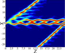
Figure 14: (Color online) The local field amplitude, $\left|u\left(X,Z\right)\right|$, in the cross section $Y=0$, for $k_{0}=1.9743$ and $\theta=\pi/8$.

A harder kick,

$$4.816<k_{0}<5.804,$$ (20)

destroys the soliton (its power at first increases, as it moves across the first PN barrier, and then decays to zero). At still higher $k_{0}$, the soliton survives the kick, but in this case its trajectory is curvilinear in the plane of $\left(X,Y\right)$as shown in Fig. 15.

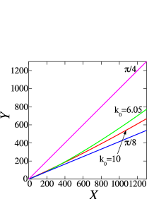
Figure 15: (Color online) Examples of curvilinear trajectories of the soliton for $\theta=\pi/8$ and two large values of the kick, $k_{0}=6.05$ and $10$. For the references, straight lines with sloped $\theta={\pi}/{8}$ and $\theta={\pi}/{4}$ are displayed too.

It is relevant to compare the number of solitons in the patterns generated by the simulations for $\theta=0$ and $\theta={\pi}/{8}$. For both cases, these numbers are presented, as functions of projection $k_{0x}\equiv k_{0}\cos\theta$ of the kick vector onto the $X$-axis, in Table 3. It is seen that the dependences of the soliton number on $k_{0x}$ are quite similar for $\theta=0$ and $\theta=\pi/8$, barring the case of the destruction of the soliton ($0$ in the table), which occurs at $\theta=\pi/8$, but does not happen for $\theta=0$.

Range of $k_{0}$	Range of the	Number of solitons	Number of solitons
	projection $k_{0x}$	$\theta=0$	$\theta={\pi}/{8}$
$[0,1.816]$	$[0,1.6778]$	1	1
$1.974$	$1.8237$	3	3
$2.1$	$1.9401$	2	2
$[2.224,4.569]$	$[2.0547,4.2212]$	1	1
$[4.816,5.804]$	$[4.4494,5.3622]$	1	0

Table 3: The number of solitons versus the $k_{0x}$ component of the kick vector, for orientations $\theta=0$ and $\pi/8$.

Further, the evolution of the soliton’s velocity for different strengths of the kick is shown in Fig. 16. Recall that, for $\theta={\pi}/{8}$, there are two domains of values of $k_{0}$ in which the kicked soliton moves, separated by interval (20) where the soliton is destroyed by the kick. It is observed that the solitons accelerate and decelerate below and above the nonexistence interval (20), respectively, but eventually the velocity approaches a constant value. Moreover, the picture suggests that, as a result of the long evolution, the velocity is pulled to either of the two discrete values, $\approx 2$ or $\approx 3$. As said above, these velocities (in other words, the values of $k_{0}$ which can directly produce such velocities, see straight horizontal lines in Fig. 16) correspond to the single soliton moving along the $X$ axis, rather than under an angle to it. The conclusion that the system relaxes to discrete values of the velocity is natural, as the dissipative system should give rise to a single or several isolated attractors, rather than a continuous family of states with an arbitrary velocity.

A similar behavior is observed for other orientations of the kick, $\theta=\pi/4$ and $\theta=0$, see the curves labeled by these values of $\theta$ in Fig. 16, and also Fig. 12. Again, the velocity asymptotically approaches the same discrete values, close to $2$ and $3$, with the acceleration or deceleration below and above these values, respectively. In the case of $\theta=\pi/4$, in the established regime the free soliton moves in the diagonal direction.

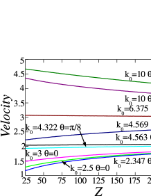
Figure 16: (Color online) The soliton’s velocity as a function of $Z$ at various values of $k_{0}$ and $\theta$.

IV Collisions between moving solitons and standing patterns

One of generic dynamical patters identified above features a standing multi-soliton structure and a freely moving soliton, which, due to the periodic boundary conditions, hits the standing structure from the opposite side, see Figs. 6, 9, 11, and 14. Two distinct scenarios of the ensuing interaction have been identified in this case, namely, the elastic collision, with the incident soliton effectively passing the quiescent structure (via a mechanism resembling the Newton’s cradle, cf. Ref. cradle ) and reappearing with the original direction and velocity of the motion, and absorption of the free soliton by the structure, see Figs. 17 and 17, respectively.

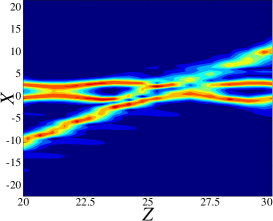
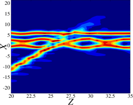
Figure 17: (Color online) Basic types of interactions between the moving soliton and the quiescent multi-soliton structure: (a) An elastic collision, at $k_{0}=1.8$ and $\theta=0$; (b) the absorption of the incident soliton, at $k_{0}=1.765$ and $\theta=0$.

More complex interaction scenarios were observed too, with several elastic or quasi-elastic collisions that end up with the eventual absorption of the free soliton. Outcomes of the collisions are summarized in Table 4 (the range of $k_{0}>2.081$ is not shown in the table, as only the single soliton exists in that case). At $1.766<k_{0}<1.86$, several elastic collisions, from $1$ to $5$, the number of which alternates in an apparently random fashion, are observed before the absorption is registered. This scenario is labeled “ Newton’s cradle with damping” in Table 4. At $k_{0}>1.86$, the collision is elastic and persists to occur periodically, as in the case of the ordinary Newton’s cradle (so named too in Table 4), see Fig. 18.

Collision type	Range of $k_{0}$
absorption	$k_{0}=1.6879$
Newton’s cradle with damping	$k_{0}=1.6909$
absorption	$k_{0}=1.692$
complex	$k_{0}=1.693$
absorption	$k_{0}\in[1.695,1.765]$
Newton’s cradle with damping	$k_{0}\in[1.766,1.86]$
Newton’s cradle	$k_{0}\in[1.866,2.081]$

Table 4: Collision types versus the magnitude of the initial kick, $k_{0}$.

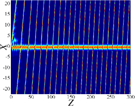
Figure 18: (Color online) An example of periodic elastic collisions according to the Newton’s-cradle scenario, at $k_{0}=1.867$ and $\theta=0$.

A special case is the one corresponding to the creation of the largest number of solitons at $k_{0}=1.693$, as shown above. The collision pattern is quite complex in this case, as shown in Fig. 19. Both elastic collisions (at $Z\simeq 50$ and $100$) and absorptions (at $Z\simeq 238$) are observed. An unexpected feature of the process is the reversal of the direction of motion of two solitons around $Z\simeq 150$. The whole patterns eventually relaxes into an array built of six solitons, which is confirmed by the power-evolution plot in Fig. 19.

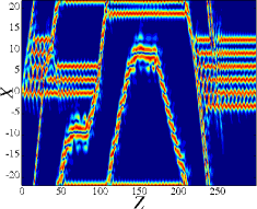
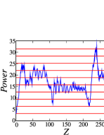
Figure 19: (Color online) (a): An example of the complex interaction of the free soliton with the standing structure at $k_{0}=1.693$ and $\theta=0$. (a) The distribution of the field, $\left|u\left(X,Z\right)\right|$, in the cross section $Y=0$; (b) the total power versus $Z$. In panel (b), horizontal lines show the multiple powers of the quiescent fundamental soliton.

In the case of elastic collisions between two solitons recurring indefinitely long, we have checked if the velocity of the transmitted soliton is the same as that of the incident one. To this end, it is relevant to consider the case of $k_{0}=1.974$ and $\theta=0$. After the first round trip of the emitted soliton, the one original is quiescent while the emitted one is running into it. It is seen in Fig. 20 that each collision leads to the exchange of velocities between the two solitons, as for colliding hard particles. In addition, we identified the velocity of the center of mass of the two-solitons set. Figure 20 shows that the latter velocity gradually increases within the sequence of collisions, approaching one of the above-mentioned discrete values characteristic to the established motion of single solitons. In the present case, the asymptotic velocity is close to $1$.

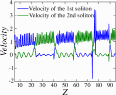
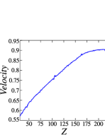
Figure 20: (Color online) Velocities of each soliton (a) and center of mass (b) versus $Z$ for the pair of periodically colliding fundamental solitons. Here $k_{0}=1.974$ and $\theta=0$.

V Conclusions

The subject of this work is the mobility of 2D dissipative solitons in the CGL (complex Ginzburg-Landau) equation which includes the spatially periodic potential. This equation models bulk lasing media with built-in transverse gratings. The soliton was set in motion by the application of the kick, which corresponds to a tilt of the seed beam Vladimirov . The mobility implies the possibility to generate oblique laser beams in the medium. Further, the advancement of the kicked soliton may be used for the controllable creation of various arrayed patterns in the wake of the soliton hopping between the potential cells. The depinning threshold, i.e., the smallest strength of the kick which sets the quiescent soliton into motion, was found by means of simulations, and also with the help of the analytical approximation, based on the estimate of the condition for the passage of the kicked object across the PN (Peierls-Nabarro) potential. The dependence of the threshold on the orientation of the kick with respect to the underlying lattice potential was studied too. Various pattern-formation scenarios have been identified above the threshold, with the number of solitons in stationary arrayed patterns varying from one to six. Freely moving solitons may eventually assume two distinct values of the velocity, which represent coexisting attractors in this dissipative system. Also studied were elastic and inelastic collisions between the free soliton and stationary multi-soliton structures, with two generic outcomes: the quasi-elastic passage, like in the case of the Newton’s cradle, and absorption of the free soliton by the quiescent structure (sometimes, after several passages). A natural extension of the present work may deal with the dynamics initiated by the application of the kick to vortices pinned by the underlying grating.

References

- (1) N. N. Rosanov, VarioSpatial Hysteresis and Optical Patterns (Springer, Berlin, 2002).
- (2) S. Barland, J. R. Tredicce, M. Brambilla, L. A. Lugiato, S. Balle, M. Giudici, T. Maggipinto, L. Spinelli, G. Tissoni, T. Knödl, M. Miller, and R. Jäger, Nature (London) 419, 699 (2002); Z. Bakonyi, D. Michaelis, U. Peschel, G. Onishchukov, and F. Lederer, J. Opt. Soc. Am. B 19, 487 (2002); E. A. Ultanir, G. I. Stegeman, D. Michaelis, C. H. Lange, and F. Lederer, Phys. Rev. Lett. 90, 253903 (2003); P. Mandel and M. Tlidi, J. Opt. B: Quantum Semiclass. Opt. 6, R60 (2004); N. N. Rosanov, S. V. Fedorov, and A. N. Shatsev, Appl. Phys. B 81, 937 (2005); C. O. Weiss and Ye. Larionova, Rep. Progr. Phys. 70, 255 (2007); N. Veretenov and M. Tlidi, Phys. Rev. A 80, 023822 (2009); P. Genevet, S. Barland, M. Giudici, and J. R. Tredicce, Phys. Rev. Lett. 104, 223902 (2010).
- (3) N. Lazarides and G. P. Tsironis, Phys. Rev. E 71, 036614 (2005); Y. M. Liu, G. Bartal, D. A. Genov, and X. Zhang, Phys. Rev. Lett. 99, 153901 (2007); E. Feigenbaum and M. Orenstein, Opt. Lett. 32, 674 (2007); I. R. Gabitov, A. O. Korotkevich, A. I. Maimistov, and J. B. Mcmahon, Appl. Phys. A 89, 277 (2007); A. R. Davoyan, I. V. Shadrivov, and Y. S. Kivshar, Opt. Exp. 17, 21732 (2009); K. Y. Bliokh, Y. P. Bliokh, and A. Ferrando, Phys. Rev. A 79, 041803 (2009); E. V. Kazantseva and A. I. Maimistov, ibid. 79, 033812 (2009); Y.-Y. Lin, R.-K. Lee, and Y. S. Kivshar, Opt. Lett. 34, 2982 (2009); A. Marini and D. V. Skryabin, ibid. 81, 033850 (2010); A. Marini, D. V. Skryabin, and B. A. Malomed, Opt. Exp. 19, 6616 (2011).
- (4) N. Akhmediev and A. Ankiewicz (Eds.), Dissipative Solitons, Lect. Notes Phys. 661, Springer, Berlin, 2005; N. Akhmediev and A. Ankiewicz (Eds.), Dissipative Solitons: From Optics to Biology and Medicine, Lect. Notes Phys. 751, Springer, Berlin, 2008.
- (5) J. Anglin, Phys. Rev. Lett. 79, 6 (1997); F. T. Arecchi, J. Bragard, and L. M. Castellano, Opt. Commun. 179, 149 (2000); J. Keeling and N. G. Berloff, Phys. Rev. Lett. 100, 250401 (2008); B. A. Malomed, O. Dzyapko, V. E. Demidov, and S. O. Demokritov, Phys. Rev. B 81, 024418 (2010); H. Deng, H. Haug, and Y. Yamamoto, Rev. Mod. Phys. 82, 1489 (2010); B. Deveaud-Plédran, J. Opt. Soc. Am. B 29, A138 (2012).
- (6) M. C. Cross and P. C. Hohenberg, Rev. Mod. Phys. 65, 851 (1993).
- (7) K.-H. Hoffmann and Q. Tang, Ginzburg-Landau Phase Transition Theory and Superconductivity (Birkhauser Verlag: Basel, 2001).
- (8) I. S. Aranson and L. Kramer, Rev. Mod. Phys. 74, 99 (2002); B. A. Malomed, in Encyclopedia of Nonlinear Science, p. 157. A. Scott (Ed.), Routledge, New York, 2005.
- (9) V. I. Petviashvili and A. M. Sergeev, Dokl. AN SSSR 276, 1380 (1984) [Sov. Phys. Doklady 29, 493 (1984)].
- (10) O. Thual and S. Fauve, J. Phys. (Paris) 49, 1829 (1988); S. Fauve and O. Thual, Phys. Rev. Lett. 64, 282 (1990); W. van Saarloos and P. C. Hohenberg, Phys. Rev. Lett. 64, 749 (1990); V. Hakim, P. Jakobsen, and Y. Pomeau, Europhys. Lett. 11, 19 (1990); B. A. Malomed and A. A. Nepomnyashchy, Phys. Rev. A 42, 6009 (1990); P. Marcq, H. Chaté, R. Conte, Physica D 73, 305 (1994); N. Akhmediev and V. V. Afanasjev, Phys. Rev. Lett. 75, 2320 (1995); H. R. Brand and R. J. Deissler, Phys. Rev. Lett. 63, 2801 (1989); V. V. Afanasjev, N. Akhmediev, and J. M. Soto-Crespo, Phys. Rev. E 53, 1931 (1996); J. M. Soto-Crespo, N. Akhmediev, and A. Ankiewicz, Phys. Rev. Lett. 85 , 2937 (2000); H. Leblond, A. Komarov, M. Salhi, A. Haboucha, and F. Sanchez, J. Opt. A: Pure Appl. Opt. 8, 319 (2006); W. H. Renninger, A. Chong, and F. W. Wise, Phys. Rev. A 77, 023814 (2008); J. M. Soto-Crespo, N. Akhmediev, C. Mejia-Cortes, and N. Devine, Opt. Express 17, 4236 (2009); D. Mihalache, Proc. Romanian Acad. A 11, 142 (2010); Y. J. He, B. A. Malomed, D. Mihalache, F. W. Ye, and B. B. Hu, J. Opt. Soc. Am. B 27, 1266 (2010); D. Mihalache, Rom. Rep. Phys. 63, 325 (2011); C. Mejia-Cortes, J. M. Soto-Crespo, R. A. Vicencio, and M. I. Molina, Phys. Rev. A 83, 043837 (2011); D. Mihalache, Rom. J. Phys. 57, 352 (2012). O. V. Borovkova, V. E. Lobanov, Y. V. Kartashov, and L. Torner, Phys. Rev. A 85, 023814 (2012).
- (11) L.-C. Crasovan, B. A. Malomed, and D. Mihalache, Phys. Rev. E 63, 016605 (2001); Phys. Lett. A 289, 59 (2001); D. Mihalache, D. Mazilu, F. Lederer, Y. V. Kartashov, L.-C. Crasovan, L. Torner, and B. A. Malomed, Phys. Rev. Lett. 97, 073904 (2006); D. Mihalache, D. Mazilu, F. Lederer, H. Leblond, and B. A. Malomed, Phys. Rev. A 76, 045803 (2007); ibid. 75, 033811 (2007); D. Mihalache and D. Mazilu, Rom. Rep. Phys. 60, 749 (2008).
- (12) M. Tlidi, M. Haelterman, and P. Mandel, Europhys. Lett. 42, 505 (1998); M. Tlidi and P. Mandel, Phys. Rev. Lett. 83, 4995 (1999); M. Tlidi, J. Opt. B: Quantum Semiclass. Opt. 2, 438 (2000).
- (13) V. Skarka and N. B. Aleksić, Phys. Rev. Lett. 96, 013903 (2006); N. B. Aleksić, V. Skarka, D. V. Timotijević, and D. Gauthier, Phys. Rev. A 75, 061802 (2007); V. Skarka, D. V. Timotijević, and N. B. Aleksić, J. Opt. A: Pure Appl. Opt. 10, 075102 (2008); V. Skarka, N. B. Aleksić, H. Leblond, B. A. Malomed, and D. Mihalache, Phys. Rev. Lett. 105, 213901 (2010).
- (14) H. Leblond, B. A. Malomed, and D. Mihalache, Phys. Rev. A 80, 033835 (2009).
- (15) A. Szameit, J. Burghoff, T. Pertsch, S. Nolte, and A. Tünnermann, Opt. Exp. 14, 6055 (2006).
- (16) J. W. Fleischer, M. Segev, N. K. Efremidis, and D. N. Christodoulides, Nature 422, 147 (2003).
- (17) W. J. Firth and A. Scroggie, Phys. Rev. Lett. 76, 1623 (1996).
- (18) M. Brambilla, A. Gatti and L. A. Lugiato, Adv. At. Molec. Opt. Phys. 40 , 229 (1998).
- (19) S. V. Fedorov, A. G. Vladimirov, G. V. Khodova, N. N. Rosanov, Phys. Rev. E 61, 5814 (2000).
- (20) D. Mihalache, D. Mazilu, V. Skarka, B. A. Malomed, H. Leblond, N. B. Aleksić, and F. Lederer, Phys. Rev. A 82, 023813 (2010).
- (21) D. Mihalache, D. Mazilu, F. Lederer, H. Leblond, and B. A. Malomed, Phys. Rev. A 81, 025801 (2010).
- (22) L. Bergé, Phys. Rep. 303, 260 (1998).
- (23) M. Desaix, D. Anderson, and M. Lisak, J. Opt. Soc. Am. B 8, 2082 (1991).
- (24) B. A. Malomed, Physica D 29, 155 (1987).
- (25) H. Sakaguchi, Physica D 210, 138 (2005).
- (26) Y. Kominis, S. Droulias, P. Papagiannis, and K. Hizanidis, Phys. Rev. A 85, 063801 (2012).
- (27) A. V. Ustinov, Phys. Lett. A 136, 155 (1989); B. A. Malomed, Phys. Rev. B 41, 26166 (1990); A. Shnirman, Z. Hermon, A. V. Ustinov, B. A. Malomed, and E. Ben-Jacob, ibid. B 50, 12793 (1994).
- (28) D. Novoa, B. A. Malomed, H. Michinel, and V. M. Pérez-García, Phys. Rev. Lett. 101, 144101 (2008)
- (29) A. G. Vladimirov, D. V. Skryabin, G. Kozyreff, P. Mandel, and M. Tlidi, Opt. Exp. 14, 1 (2006).