Symmetric discrete coherent states for $n$ qubits

Abstract

We put forward a method of constructing discrete coherent states for $n$ qubits. After establishing appropriate displacement operators, the coherent states appear as displaced versions of a fiducial vector that is fixed by imposing a number of natural symmetry requirements on its $Q$ function. Using these coherent states we establish a partial order in the discrete phase space, which allows us to picture some $n$-qubit states as apparent distributions. We also analyze correlations in terms of sums of squared $Q$ functions.

1 Introduction

Coherent states (CS), first introduced by Schrödinger [1], are of paramount significance for modern physical theories, as they are quantum states that follow classical trajectories. In quantum optics, CS were popularized by Glauber [2, 3] for the description of correlation properties of a single-mode radiation field, where the Weyl-Heisenberg group emerges as a hallmark of noncommutativity [4].

Although generalizations along several directions have been considered (see references  [5, 6, 7] for reviews), nowadays it seems indisputable that the pioneer work of Perelomov [8] paved the way to extend the notion of CS to quantum systems with dynamical symmetry group $G$. In this approach, CS appear as orbits of a certain fiducial state under a unitary irreducible representation of $G$ acting in the corresponding Hilbert space.

This fiducial state is chosen to have maximal isotropy subgroup $H$, which ultimately leads to “maximal classicality”. Under these circumstances, the displacement operators, transforming CS among themselves, are labeled by points in the manifold $M=G/H$. For many physical models, $M$ can be equipped with an irreducible symplectic structure [9, 10, 11, 12], so it can be considered as the phase space of a classical dynamical system. In other words, there is a one-to-one correspondence between CS and points of the classical phase space.

The crucial point of this construction is that the Hilbert space is irreducible under the action of $G$. This is especially clear for the symmetric representations of the unitary groups $SU(n)$, when the classical phase space is a $(2n-2)$-dimensional sphere [13]. For the discrete counterparts, even in the physically (but not mathematically!) simple $n$-qubit case, the symmetric subspace is only a very small portion of the whole $2^{n}$-dimensional Hilbert space. Nonetheless, one can define a natural set of CS, constructed in a similar way as in the continuous case: acting on a fiducial state with discrete displacements; i.e., unitary operators labeled by elements of two discrete sets [14]. These two sets can be organized in a discrete $2^{n}\times 2^{n}$ grid, on which a specific discrete geometry (including symplectic operations) can be introduced, so that such a grid turns out to be a bona fide discrete phase space [15, 16, 17, 18, 19, 20, 21, 22, 23].

Although the points of the discrete phase space label again CS, there is still an essential difference with the continuous case: the choice of the fiducial state. For continuous symmetry groups, the standard choice corresponds to an extreme state of the representation, such as the vacuum or the lowest/highest weight state. In the discrete case, the nature of the unitary displacements prevents such a simple notion and different possibilities have been discussed so far [24, 25].

In this paper, we take the fiducial state as a spin CS and impose that its associated $Q$ function fulfills reasonable symmetry conditions. This not only solves the problem, but allows us to use the system of CS to impose a partial order in phase space, which helps to recognize states pictured as distributions. Finally, we briefly speculate about detecting quantum correlations through the sum of squared $Q$ functions.

2 Discrete phase space

A qubit is a two-dimensional quantum system, with Hilbert space isomorphic to $\mathbb{C}^{2}$. It is customary to choose two normalized orthogonal states, $\{|0\rangle,|1\rangle\}$, as a computational basis. The unitary operators

$$\sigma_{z}=|0\rangle\langle 0|-|1\rangle\langle 1|\,,\qquad\qquad\sigma_{x}=|0\rangle\langle 1|+|1\rangle\langle 0|\,.$$ (2.1)

generate the Pauli group $\mathcal{P}_{1}$ under matrix multiplication [26].

For $n$ qubits, the Hilbert space is the tensor product $\mathbb{C}^{2}\otimes\cdots\otimes\mathbb{C}^{2}=\mathbb{C}^{2^{n}}$. A compact way of labeling both states and elements of the corresponding Pauli group $\mathcal{P}_{n}$ consists in using the finite field $\mathbb{F}_{2^{n}}$ [27]. This can be considered as a linear space spanned by an abstract basis $\{\theta_{1},\ldots,\theta_{n}\}$, so that given a field element $\alpha$ (henceforth, field elements will be denoted by Greek letters) the expansion

$$\alpha=\sum_{i=1}^{n}a_{i}\,\theta_{i}\,,\qquad a_{i}\in\mathbb{Z}_{2}\,,$$ (2.2)

allows us the identification $\alpha\Leftrightarrow(a_{1},\ldots,a_{n})$. Moreover, the basis can be chosen to be orthonormal with respect to the trace operation (the self-dual basis); that is,

$$\tr(\theta_{i}\,\theta_{j})=\delta_{ij}\,,$$ (2.3)

where $\tr(\alpha)=\alpha+\alpha^{2}+\ldots+\alpha^{2^{n-1}}$, which actually maps $\mathbb{F}_{2^{n}}\mapsto\mathbb{Z}_{2}$. In this way, we associate each qubit with a particular element of the self-dual basis: qubit${}_{i}\Leftrightarrow\theta_{i}$.

The generalized Pauli group $\mathcal{P}_{n}$ is generated now by the operators

$$Z_{\alpha}=\sum_{\lambda}\chi(\alpha\lambda)\,|\lambda\rangle\langle\lambda|\,,\qquad\qquad X_{\beta}=\sum_{\lambda}|\lambda+\beta\rangle\langle\lambda|\,.\\$$ (2.4)

Here the additive characters $\chi$ are defined as $\chi(\alpha)=\exp[i\pi\tr(\alpha)]$ and $|\lambda\rangle$ is an orthonormal basis in the Hilbert space of the system. Operationally, the elements of the basis can be labeled by powers of a primitive element (i.e., a root of the primitive polynomial), and read $\{|0\rangle,\,|\sigma\rangle,\ldots,\,|\sigma^{2^{n}-1}=1\rangle\}$. One can verify that

$$Z_{\alpha}X_{\beta}=\chi(\alpha\beta)\,X_{\beta}Z_{\alpha}\,,$$ (2.5)

which is the discrete counterpart of the Weyl-Heisenberg algebra for continuous variables [4].

The operators (2.4) can be factorized into tensor products of powers of single-particle Pauli operators. This factorization can be carried out by mapping each element of $\mathbb{F}_{2^{n}}$ onto an ordered set of natural numbers according to

$$Z_{\alpha}=\sigma_{z}^{a_{1}}\otimes\ldots\otimes\sigma_{z}^{a_{n}},\qquad\qquad X_{\beta}=\sigma_{x}^{b_{1}}\otimes\ldots\otimes\sigma_{x}^{b_{n}}\,,$$ (2.6)

where $a_{i}=\tr(\alpha\theta_{i})$ and $b_{i}=\tr(\beta\theta_{i})$ are the corresponding expansion coefficients for $\alpha$ and $\beta$ in the self-dual basis. Moreover, they are related through the finite Fourier transform [28]

$$\mathcal{F}=\frac{1}{\sqrt{2^{n}}}\sum_{\lambda,\lambda^{\prime}}\chi(\lambda\,\lambda^{\prime})\,|\lambda\rangle\langle\lambda^{\prime}|\,,$$ (2.7)

so that $X_{\mu}=\mathcal{F}Z_{\mu}\,\mathcal{F}$.

We next recall [20] that the grid defining the phase space for $n$ qubits can be appropriately labeled by the discrete points $(\alpha,\beta)$, which are precisely the indices of the operators $Z_{\alpha}$ and $X_{\beta}$: $\alpha$ is the “horizontal” axis and $\beta$ the “vertical” one. In this grid one can introduce the concept of straight lines (also called rays), which possess the same properties as in the continuous case. It is worth noting that the monomials labeled by points of the same ray, $\{(\alpha,\mu\alpha)\}$ commute with each other, so that one can establish a correspondence between eigenstates of such commuting sets and states (actually bases) in the Hilbert space [20].

Following our program, we introduce the set of displacements

$$D(\alpha,\beta)=e^{i\Phi(\alpha,\beta)}\,Z_{\alpha}X_{\beta}\,,$$ (2.8)

where $\Phi(\alpha,\beta)$ is a phase required to avoid plugging extra factors when acting with $D$. One can immediately check that

$$D(\alpha,\beta)D^{{\dagger}}(\alpha,\beta)=\leavevmode\hbox{\small 1\normalsize\kern-3.30002pt1},\quad D^{{\dagger}}(\alpha,\beta)=D(\alpha,\beta)\,,$$ (2.9)

so they are unitary and Hermitian. They also constitute a complete trace-orthonormal set

$$\Tr[D(\alpha,\beta)\,D(\alpha^{\prime},\beta^{\prime})]=2^{n}\delta_{\alpha\alpha^{\prime}}\delta_{\beta\beta^{\prime}}\,.$$ (2.10)

These operators act multiplicatively on the monomials (2.4), thus shifting phase-space points according to

$$(\alpha,\beta)\overset{D(\alpha^{\prime},\beta^{\prime})}{\mapsto}(\alpha+\alpha^{\prime},\beta+\beta^{\prime})\,,$$ (2.11)

which justifies their designation.

Finally, for later purposes, we touch on a pair of symplectic operations ($z$- and $x$-rotations) that transform rays into rays according to

$$P_{\mu}Z_{\alpha}P_{\mu}^{\dagger}\propto Z_{\alpha}X_{\mu\alpha}\,,\qquad\qquad Q_{\nu}X_{\beta}Q_{\nu}^{\dagger}\propto Z_{\nu\beta}X_{\beta}\,.$$ (2.12)

The symbol $\propto$ indicates equality except for a phase. Both $P_{\mu}$ and $Q_{\nu}$ are unitary operators, with $[P_{\mu},X_{\nu}]=[Q_{\nu},Z_{\mu}]=0$, and can be written as

$$P_{\mu}=\sum_{\lambda}c_{\lambda,\mu}|\widetilde{\lambda}\rangle\langle\widetilde{\lambda}|\,,\qquad\qquad Q_{\nu}=\sum_{\lambda}c_{\lambda,\nu}|\lambda\rangle\langle\lambda|\,,$$ (2.13)

where $|\lambda\rangle$ are the eigenstates of $Z_{\alpha}$ and $|\widetilde{\lambda}\rangle$ of $X_{\beta}$. The coefficients $c_{\lambda,\nu}$ fulfill the recurrence relation

$$c_{\lambda+\alpha,\nu}=c_{\alpha,\nu}c_{\lambda,\nu}\,\chi(\nu\alpha\lambda),\qquad\qquad c_{0,\nu}=1\,,$$ (2.14)

whose explicit solution can be found in reference [29] and it is unimportant for the rest of the paper.

We associate an eigenstate $|\psi_{0}\rangle$ of $Z_{\alpha}$ with the horizontal axis and immediately obtain that the state associated with the ray $\beta=\mu\alpha$ is $P_{\mu}|\psi_{0}\rangle$, while the vertical axis is associated with $\mathcal{F}|\psi_{0}\rangle$ [30] . Any other straight line, parallel to a given ray, but crossing the axis $\beta$ at the point $\beta=\xi$, corresponds to the state $X_{\xi}P_{\mu}|\psi_{0}\rangle$.

Using phase-space coordinates these $z$- and $x$-rotations can be interpreted as

$$(\alpha,\beta)\overset{P_{\mu}}{\mapsto}(\alpha,\beta+\mu\alpha)\,,\qquad\qquad(\alpha,\beta)\overset{Q_{\nu}}{\mapsto}(\alpha+\nu\beta,\beta)\,.$$ (2.15)

It is clear that these two transformations are conjugate each other.

3 Discrete coherent states for $n$ qubits

According to the conventional approach, we define discrete CS $|\alpha,\beta\rangle$, labeled by phase-space points $(\alpha,\beta)$, as the displacements of the fiducial state $|\Psi_{0}\rangle$ [19]:

$$|\alpha,\beta\rangle=D(\alpha,\beta)|\Psi_{0}\rangle\,.$$ (3.1)

The state $|\Psi_{0}\rangle$ can be chosen in several ways [24]. Here, for reasons that will be apparent soon, we take $|\Psi_{0}\rangle$ as a product of identical qubit states:

$$|\Psi_{0}\rangle=|\vartheta,\varphi\rangle_{1}\otimes\cdots\otimes|\vartheta,\varphi\rangle_{n}\,,$$ (3.2)

where

$$|\vartheta,\varphi\rangle_{j}=e^{i\varphi/2}\sin\left(\frac{\vartheta}{2}\right)|1\rangle_{j}+e^{-i\varphi/2}\cos\left(\frac{\vartheta}{2}\right)|0\rangle_{j}\,,$$ (3.3)

and the angles $(\vartheta,\varphi)$ parametrize the Bloch sphere. The state (3.2) is invariant under permutation of the qubit indices and thus can be expanded as [24]

$$|\Psi_{0}\rangle\equiv|\xi\rangle=\frac{1}{(1+|\xi|^{2})^{n/2}}\sum_{k=0}^{n}\sqrt{\frac{n!}{k!(n-k)!}}\,\xi^{k}|k,n\rangle\,,$$ (3.4)

with $\xi=e^{i\varphi}\,\tan\vartheta/2$. The basis $\{|k,n\rangle\,:\,k=0,\ldots,n\}$ are the Dicke states

$$|k,n\rangle=\sqrt{\frac{k!(n-k)!}{n!}}\sum_{k=0}^{n}\mathcal{P}_{k}|(|1\rangle_{1}\ldots|1\rangle_{k}|0\rangle_{k+1}\ldots|0\rangle_{n})\,.$$ (3.5)

Here, $\{\mathcal{P}_{k}\}$ denotes the complete set of all the possible qubit permutations.

In field notation, the state (3.4) can be compactly expressed as

$$|\xi\rangle=\frac{1}{(1+|\xi|^{2})^{n/2}}\sum_{\kappa}\xi^{h(\kappa)}|\kappa\rangle\,,$$ (3.6)

where the function $h(\kappa)$ counts the number of nonzero coefficients $k_{j}$ in the expansion of $\kappa$ in the field basis (see the appendix for a brief account of its properties).

Finally, notice that one might think in imposing that the states $|\xi\rangle$ are eigenstates of the Fourier operator [31, 32] (much as the vacum is for continuous variables). Since $\mathcal{F}^{2}=\leavevmode\hbox{\small 1\normalsize\kern-3.30002pt1}$, this is tantamount to

$$\mathcal{F}|\xi\rangle=\pm|\xi\rangle\,,$$ (3.7)

which leads to two possible candidates $\xi_{\pm}=\pm\sqrt{2}-1$ and all the qubits pointing in the same direction. However, we prefer to follow an alternative route to fix the possible values of $\xi$.

3.1 $P$-function

Let us look for an expansion of the density matrix of the form

$$\varrho=\sum_{\alpha,\beta}P(\alpha,\beta)|\alpha,\beta\rangle\langle\alpha,\beta|\,,$$ (3.8)

which is the analogous to the Glauber-Sudarshan $P$-function for continuous variables [33, 34]. It is not difficult to check that the function $P(\alpha,\beta)$ may be recast as

$$P(\alpha,\beta)=\Tr[\varrho\Delta(\alpha,\beta)]\,,$$ (3.9)

where $\Tr$ (with capital T to distinguish it from $\tr$, which is the trace in the field) stands for the ordinary trace operation in Hilbert space. The kernel $\Delta(\alpha,\beta)$ reads

$$\Delta(\alpha,\beta)=\frac{1}{2^{2n}}\sum_{\gamma,\delta}\chi(\alpha\delta+\beta\gamma)\,\langle\xi|D(\gamma,\delta|\xi\rangle^{-1}D(\gamma,\delta)\,.$$ (3.10)

This clearly shows that the $P$-function is nonsingular only when $\langle\xi|D(\gamma,\delta)|\xi\rangle^{-1}$ exists.

Since the state $|\xi\rangle$ is factorized into single-qubit states, we have

$$\langle\xi|D(\gamma,\delta)|\xi\rangle\propto\prod_{i=1}^{n}\langle\xi^{(1)}|\sigma_{z}^{g_{i}}\sigma_{x}^{d_{i}}|\xi^{(1)}\rangle\,,$$ (3.11)

where $g_{i},d_{i}$ are the expansion coefficients of $\gamma$ and $\delta$ in the self-dual basis and

$$|\xi^{(1)}\rangle=\frac{1}{\sqrt{1+|\xi|^{2}}}(|0\rangle+\xi|1\rangle)\,.$$ (3.12)

Using equation (3.6) one can find

$$\langle\xi|D(\gamma,\delta)|\xi\rangle \propto \left(\frac{1-|\xi|^{2}}{1+|\xi|^{2}}\right)^{[h(\gamma)-h(\delta)+h(\gamma+\delta)]/2}$$ (3.13)

$$\times \left(\frac{\xi+\xi^{\ast}}{1+|\xi|^{2}}\right)^{[h(\delta)-h(\gamma)+h(\gamma+\delta)]/2}\left(\frac{\xi-\xi^{\ast}}{1+|\xi|^{2}}\right)^{[h(\gamma)+h(\delta)-h(\gamma+\delta)]/2}\,.$$

This obviously rules out some values of $\xi$ for which $P$ is singular.

As an illustrative example, consider the case of a single qubit. Then, one finds that

$$P(a,b)=\frac{1}{4}+\frac{1+|\xi|^{2}}{4}\left[(-1)^{b}\frac{\Tr(\varrho\sigma_{z})}{1-|\xi|^{2}}+(-1)^{a}\frac{\Tr(\varrho\sigma_{x})}{\xi+\xi^{\ast}}+(-1)^{a+b}\frac{\Tr(\varrho\sigma_{z}\sigma_{x})}{\xi-\xi^{\ast}}\right]\,,$$ (3.14)

where now $a,b\in\mathbb{Z}_{2}$. This function is singular when $\xi$ is real, imaginary, and when $|\xi|^{2}=1$, i.e. on the equator of the Bloch sphere. In particular, the eigenstates of the discrete Fourier transform, when $\xi_{\pm}=\sqrt{2}\pm 1$, do not lead to the faithful expansion on CS for qubits, contrary to what one could expect.

3.2 $Q$-function

In our search for determining the values of $\xi$, we next look at the $Q$-function, defined in complete analogy with its continuous counterpart, namely

$$Q_{\varrho}(\alpha,\beta)=\langle\alpha,\beta|\varrho|\alpha,\beta\rangle\,,$$ (3.15)

which satisfies

$$\sum_{\alpha,\beta}Q_{\varrho}(\alpha,\beta)=2^{n}\,.$$ (3.16)

Let us impose the maximal symmetry conditions admissible on the $Q$-function for the fiducial state $|\xi\rangle$:

C1

.- $Q_{|\xi\rangle}(\alpha,\beta)$ is symmetric under axis permutations.

C2

.- The values of $Q_{|\xi\rangle}(\alpha,\beta)$ can be obtained from $Q_{|\xi\rangle}(\alpha,0)$ by $z$- and $x$- rotations.

Since $Q_{|\xi\rangle}(\alpha,\beta)=|\langle\xi|D(\alpha,\beta)|\xi\rangle|^{2}$, and using equation (3.13), one can easily find out that the condition C1 [$Q_{|\xi\rangle}(\alpha,\beta)=Q_{|\xi\rangle}(\beta,\alpha)$] imposes the following restriction on $\xi$ (this is one of the possible restrictions, but the other ones are just symmetric reflections):

$$\xi=\left(\sqrt{1+\cos^{2}\vartheta}-\cos\vartheta\right)\exp(i\vartheta)\,,\qquad-\pi/2<\vartheta<\pi/2\,,$$ (3.17)

so that the $Q$-function takes the form

$$Q_{|\xi\rangle}(\alpha,\beta)=\left(\frac{\cos\vartheta}{\sqrt{1+\cos^{2}\vartheta}}\right)^{2h(\alpha+\beta)}\left(\frac{\sin\vartheta}{\sqrt{1+\cos^{2}\vartheta}}\right)^{[h(\alpha)+h(\beta)-h(\alpha+\beta)]}\,.$$ (3.18)

To fulfill the condition C2, we first require that $Q_{|\xi\rangle}(\alpha,0)$ contains all the possible values of $Q_{|\xi\rangle}(\alpha,\beta)$. To this end, we note that

$$Q_{|\xi\rangle}(\kappa,\kappa)=\left(\frac{\sin\vartheta}{\sqrt{1+\cos^{2}\vartheta}}\right)^{2h(\kappa)}\,,\qquad\qquad Q_{|\xi\rangle}(\alpha,0)=\left(\frac{\cos\vartheta}{\sqrt{1+\cos^{2}\vartheta}}\right)^{2h(\alpha)}\,,$$ (3.19)

so that the only possibility (apart from symmetric reflections) is that $\sin\vartheta=\cos\vartheta$, i.e. $\vartheta=\pi/4$. Consequently, equation (3.18) takes the simple form

$$Q_{|\xi\rangle}(\alpha,\beta)=\left(\frac{1}{\sqrt{3}}\right)^{[h(\alpha)+h(\beta)+h(\alpha+\beta)]}\,,$$ (3.20)

which explicitly fulfills $Q_{|\xi\rangle}(\alpha,\alpha)=Q_{|\xi\rangle}(\alpha,0)$.

Using the properties of the function $h$ (see appendix A), one can infer that for any ordered pair $(\alpha,\beta)$ there is always a field element $\kappa$, given by

$$\kappa=\sum_{i=1}^{n}(a_{i}+b_{i}-a_{i}b_{i})\,\theta_{i}\,,$$ (3.21)

$\{\theta_{i}\}$ being the self-dual basis, such that $Q_{|\xi\rangle}(\alpha,\beta)=Q_{|\xi\rangle}(\kappa,0)$. This means that each value of $Q_{|\xi\rangle}(\alpha,\beta)$ can be obtained by rotating $Q_{|\xi\rangle}(\kappa,0)$ according to the following protocol:

$$(\kappa,0)\overset{P_{\mu}}{\mapsto}(\kappa,\mu\kappa)\overset{Q_{\nu}}{\mapsto}(\kappa+\kappa\mu\nu,\kappa\mu)\,,$$ (3.22)

where the rotation parameters are $\mu=\beta\kappa^{-1}$ and $\nu=(\alpha+\kappa)\beta^{-1}$.

To conclude, we observe that, for a single qubit, the $P$-function (3.14) for the value $\xi$ in equation (3.17) (at $\vartheta=\pi/4$), becomes

$$P(a,b)=\frac{1}{4}+\frac{\sqrt{3}}{4}\left[(-1)^{b}\Tr(\varrho\sigma_{z})+(-1)^{a}\Tr(\varrho\sigma_{x})+(-1)^{a+b}\Tr(\varrho\sigma_{y})\right]\,.$$ (3.23)

which is the most uniform possible. Note, in passing, that this maximum uniformity could be also adopted as a reasonable criterion to fix the value of $\xi$. The associated unit vector clearly reflects this uniformity

$$\mathbf{n}=(\langle\xi|\sigma_{x}|\xi\rangle,\langle\xi|\sigma_{y}|\xi\rangle,\langle\xi|\sigma_{z}|\xi\rangle)=1/\sqrt{3}\,(1,1,1)\,.$$ (3.24)

4 Ordering points in the discrete phase space

The very simple form of the $Q$-function for the fiducial state $|\xi\rangle$ in the previous section allows to introduce a partial order in the $n$-qubit phase space. Indeed, since any $Q_{|\xi\rangle}(\alpha,\beta)$ can be obtained by rotations from $Q_{|\xi\rangle}(\kappa,0)=3^{-h(\kappa)}$, we can order the points on the horizontal axis according to the values of the $h$-function: $0\leq h(\alpha)=k\leq n$. The $C_{k}^{n}=\frac{n!}{k!(n-k)!}$ elements which correspond to the same value of the $h$-function remain disordered inside the strip with the fixed value of $h(\alpha)=k$. This automatically arranges the rest of the phase-space points according to the symmetry property and the construction (3.22).

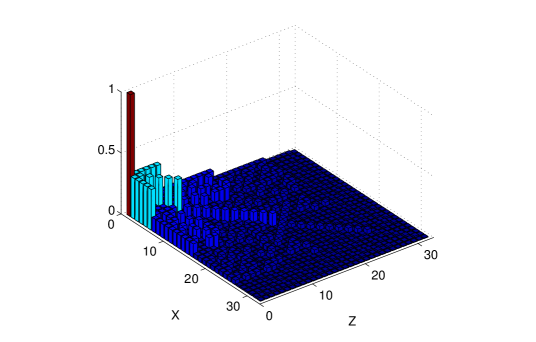
Figure 1: Ordered Q-function for the fiducial state $|\xi\rangle$.

In figure 1 we plot the $Q$-function for the fiducial state $|\xi\rangle$ for 5 qubits using this ordering. Explicitly, the order of axis is chosen as: $0$, $\sigma^{6}$, $\sigma^{26}$, $\sigma$, $\sigma^{7}$, $\sigma^{2}$, $\sigma^{16}$, $\sigma^{27}$, $\sigma^{8}$, $\sigma^{17}$, $\sigma^{18}$, $\sigma^{3}$, $\sigma^{19}$, $\theta^{20}$, $\theta^{9}$, $\theta^{28}$, $\theta^{10}$, $\sigma^{21}$, $\sigma^{22}$, $\sigma^{29}$, $\sigma^{23}$, $\sigma^{24}$, $\sigma^{4}$, $\sigma^{11}$, $\sigma^{5}$, $\sigma^{12}$, $\sigma^{25}$, $\sigma^{13}$, $\sigma^{14}$, $\sigma^{30}$, $\sigma^{15}$, $\sigma^{31}$. The irreducible polynomial used is $x^{5}+x^{2}+1=0$, and the self-dual basis chosen for $\mathbb{F}_{2^{5}}$ is $\theta_{1}=\sigma^{3},\theta_{1}=\sigma^{5},\theta_{1}=\sigma^{11},\theta_{1}=\sigma^{22},\theta_{1}=\sigma^{24}$.

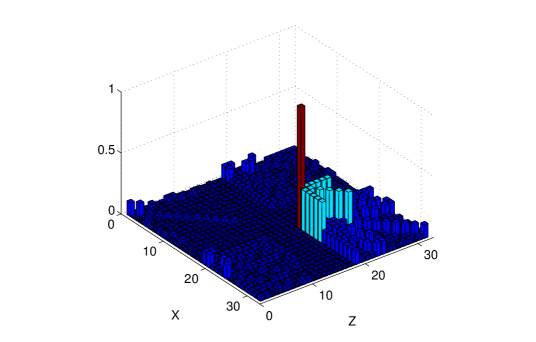
Figure 2: Properly ordered Q-function for the state $|\theta^{10},\theta^{10}\rangle$.

The shape of the $Q$-function presents a hump localized at the origin. Due to the covariance under displacements, $Q_{|\gamma,\delta\rangle}(\alpha,\beta)=Q_{|\xi\rangle}(\alpha+\gamma,\beta+\delta)$, the ordering should be applied to the pairs $(\alpha+\gamma,\beta+\delta)$, but not to $(\alpha,\beta)$ itself. In this sense, one cannot properly say that $Q_{|\gamma,\delta\rangle}(\alpha,\beta)$ has a hump located at $(\gamma,\delta)$ if we keep the previously established order. Nonetheless, it is clear that due to the functional form of $Q_{|\gamma,\delta\rangle}(\alpha,\beta)$ the elements of the field can be easily rearranged (using the summation table) in a such way that the corresponding hump becomes centered at $(\gamma,\delta)$ and has a symmetric form. In figure 2 we plot the $Q$-function for the - qubit CS $|\theta^{10},\theta^{10}\rangle=D(\theta^{10},\theta^{10})|\xi\rangle$ according to such a prescription.

It is also worth observing that the $Q$-function of an arbitrary state $|\Psi\rangle$ can be written down as

$$Q_{|\Psi\rangle}(\alpha,\beta)=\sum_{\gamma,\delta}P(\alpha+\gamma,\beta+\delta)\,Q_{|\xi\rangle}(\gamma,\delta)\,,$$ (4.1)

i.e. as an smearing of the $P$-function. In particular, the order established by the $h$-function helps to visualize the superpositions of several discrete CS as spatially separated humps in phase space. In figure 3 we plot the $Q$-function for a superposition of two CS for 5 qubits, $|\Psi\rangle\propto(|\xi\rangle+D(\theta^{31},\theta^{31})|\xi\rangle)$, and the ordering is the same as for $Q_{|\xi\rangle}$. We can clearly observe two humps with a residual symmetry.

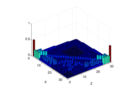
Figure 3: Q-function for the state $|\psi\rangle\propto(|\xi\rangle+D(\theta^{31},\theta^{31})|\xi\rangle)$.

As a final remark we may note that the distribution still can be re-ordered in a more symmetric form just distributing the points with the same value of $h(\alpha)$ on both sides of the principal peak. Although the number of such points is not always even, for a large number of qubits the distribution corresponding to the CS is practically symmetric, as it can be seen from figure 4, where we plot the $Q$-function for the fiducial state $|\xi\rangle$ corresponding to 8 qubits.

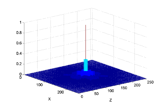
Figure 4: Ordered symmetrized $Q$-function of the fiducial coherent state $|\xi\rangle$ displaced to the center of the phase-space for eight qubits.

It is worth comparing the form of the $Q$-function for the $n$-qubit CS (3.1) in the limit $n\gg 1$ with the CS resulting from taking as the fiducial state an eigenstate of the discrete Fourier transform [31] . In the latter case the $Q$-function tends to a Gaussian shape [19] , while in our approach it has a step form modulated by a decreasing function $f(k)$, which along the axes $Z$ ($\beta=0$), $X$ ($\alpha=0$) and $Y$ ($\alpha=\beta$) has an exponential form:

$$f(k)=\delta_{k0}+3^{-k}\sum_{m=0}^{n-1}\left[\theta\left(k-\sum_{r=0}^{m}C_{r}^{n}\right)-\theta\left(k-\sum\limits_{r=0}^{m+1}C_{r}^{n}\right)\right]\,,$$ (4.2)

where $\theta\left(k\right)$ is the Heaviside step function.

5 Detecting correlations in $n$-qubit systems

By construction, the discrete CS are factorized states, so the qubits therein do not exhibit correlations. For symmetric states, the correlations are frequently measured using the concept of spin squeezing [35, 36, 37, 38, 39, 40], comparing the fluctuations of some definite operator with the standard quantum limit, given by the spin CS. Nevertheless, for nonsymmetric states similar criteria do not work well [41] for the choice of the measured operators becomes nontrivial.

To study correlations in nonsymmetric $n$-qubit states we apply a criteria proposed in reference [42] to quantify polarization fluctuations. According to this approach, we compute the sum of squares of the $Q$-function: quantum correlations make such a sum lesser than the corresponding one for a CS. In fact, for the fiducial state $|\xi\rangle$ we have

$$\sum_{\alpha,\beta}Q_{|\xi\rangle}^{2}(\alpha,\beta)=\sum_{\alpha,\beta}\left(\frac{1}{3}\right)^{[h(\alpha)+h(\beta)+h(\alpha+\beta)]}=\prod_{i=1}^{n}\sum_{a_{i},b_{i}=0}^{1}\left(\frac{1}{3}\right)^{[2a_{i}+2b_{i}-2a_{i}b_{i}]}=\left(\frac{4}{3}\right)^{n}\,.$$ (5.1)

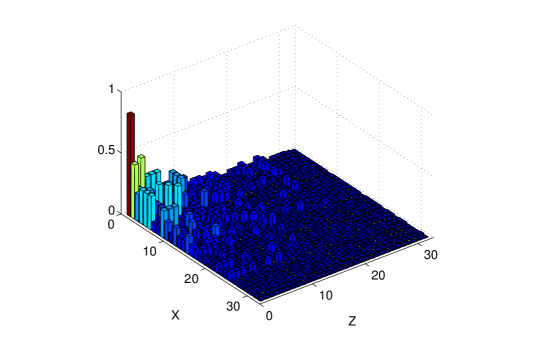
Figure 5: Q-function for the state $\mbox{{xor}}_{1,2}|\xi\rangle$.

To check the method, we consider a simple way to induce correlations between qubits: the application if $\mbox{{xor}}_{p,q}$ gates, where the pair $(p,q)$ indicates the qubits on which the operator is applied, namely

$$\mbox{{xor}}_{p,q}|a_{1},\ldots,a_{p},\ldots,a_{q},\ldots,a_{n}\rangle=|a_{1},\ldots,a_{p},\ldots,a_{q}+a_{p},\ldots,a_{n}\rangle\,.$$ (5.2)

For a correlated state $|\Psi\rangle=\mbox{{xor}}_{p,q}D(\mu,\nu)|\xi\rangle$ the sum of $Q^{2}$ curiously does not depend on the form of the displacement $D(\mu,\nu)$ and gives

$$\sum_{\alpha,\beta}Q_{|\Psi\rangle}^{2}(\alpha,\beta)=\frac{128}{81}\left(\frac{4}{3}\right)^{n-2}\,,$$ (5.3)

which is smaller than (5.1). In the same vein, the application of $k$ xor gates between different particles (i.e., now $|\Psi\rangle=\mbox{{xor}}_{p_{k},q_{k}}\ldots\mbox{{xor}}_{p_{1},q_{1}}D(\mu,\nu)|\xi\rangle$, with $p_{1}\neq q_{1}\neq\ldots\neq p_{k}\neq q_{k}$) keeps decreasing the sum:

$$\sum_{\alpha,\beta}Q_{|\Psi\rangle}^{2}(\alpha,\beta)=\left(\frac{128}{81}\right)^{k}\left(\frac{4}{3}\right)^{n-2k}\,.$$ (5.4)

Similarly, the application of sequences of xor gates to the fiducial state also leads to decreasing values of the $\sum Q^{2}(\alpha,\beta)$. This effect can be clearly seen in figure 5, where the $Q$-function for the state $\mbox{{xor}}_{1,2}|\xi\rangle$ is plotted. One can observe that the heights of the $Q(\alpha,\beta)$ are smaller, so that the distribution initially localized at the origin sparse over a substantial part of the phase space.

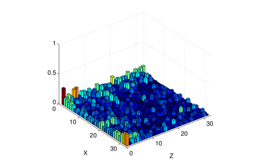
Figure 6: $Q$-function of the squeezed state $S_{\sigma^{7}}|\xi\rangle.$

To induce correlation between all the qubits in a regular way one can apply the squeezing operator [21, 25]

$$S_{\zeta}=\sum_{\lambda}|\lambda\rangle\langle\zeta\lambda|\,,$$ (5.5)

which acts on the $Z_{\alpha}$ and $X_{\beta}$ as the scaling transformation

$$S_{\zeta}\,X_{\beta}S_{\zeta}^{\dagger}=X_{\beta\zeta}\,,\qquad\qquad S_{\zeta}\,Z_{\alpha}S_{\zeta}^{\dagger}\,=Z_{\alpha\zeta^{-1}}\,,$$ (5.6)

much as in the continuous case. The action of (5.5) on a CS can be formally expressed as

$$S_{\zeta}|\xi\rangle=\frac{1}{(1+|\xi|^{2})^{n/2}}\sum_{\kappa}\xi^{h(\zeta\kappa)}|\kappa\rangle\,,$$ (5.7)

and implies that the initially factorized state (3.2) is transformed into

$$S_{\zeta}|\xi\rangle=\frac{1}{(1+|\xi|^{2})^{n/2}}\sum_{k_{1},\ldots,k_{n}}\xi^{\sum_{j=1}^{n}k_{j}d_{j}}\,|k_{1},\ldots,k_{n}\rangle\,,$$ (5.8)

where

$$d_{j}=\sum_{i,m=1}^{n}f_{ijm}c_{m}\,,\qquad c_{m}=\tr(\zeta\theta_{m})\,,\qquad f_{ijm}=\tr(\theta_{i}\theta_{j}\theta_{m})\,.$$ (5.9)

The squeezing operator $S_{\zeta}$ correlates all the qubits in a generic CS (3.1) and the degree of such correlation depends both on $\xi$ and $\zeta$. For example, in the 5-qubit case the operator $\hat{S}_{\sigma^{7}}$ correlates qubits in the initial CS with $\xi=e^{\pi i/4}\left(\sqrt{3}-1\right)/\sqrt{2}$ in the most efficient way according to the criteria (5.1), and its action on the fiducial state $|\xi\rangle$ is

$$S_{\sigma^{7}}|\xi\rangle = \frac{1}{(1+|\xi|^{2})^{5/2}}\sum_{k_{i}}\xi^{\{k_{4}+k_{5}\}}\xi^{\{k_{2}+k_{3}+k_{4}+k_{5}\}}\xi^{\left\{k_{2}+k_{4}\right\}}$$ (5.10)

$$\times \xi^{\left\{k_{1}+k_{2}+k_{3}+k_{4}\right\}}\xi^{\left\{k_{1}+k_{2}+k_{5}\right\}}|k_{1},k_{2},k_{3},k_{4},k_{5}\rangle\,,$$

and $\{.+.\}$ means sum $\bmod\ 2$. In figure 6 we plot the $Q$-function of the state $\hat{S}_{\sigma^{7}}|\xi\rangle$, where it can be observed that the initial distribution is spread out over practically all the phase space.

6 Conclusions

We have developed a method for constructing discrete CS from the symmetry conditions for the $Q$-function of the fiducial state. This has allowed us to order the points in the discrete phase space. Besides, we have applied a criterion for the detection of quantum correlations to the discrete case and have shown that it can be useful for $n$-qubit systems.

Appendix A Some properties of the function $h(\alpha)$

The function $h(\alpha)$ is defined as the number of nonzero components in the expansion of a field element $\alpha$ in the self-dual basis $\{\theta_{i}\}$, that is

$$h(\alpha)=\sum_{i=1}^{n}a_{i}\,,$$ (1.1)

where $a_{i}=\tr(\alpha\theta_{i})$. Note that $0\leq h(\alpha)\leq n$. The basic properties we need in this paper are the following:

$$\sum_{i=1}^{n}\chi(\alpha\sigma_{i}) = \sum_{i=1}^{n}(-1)^{a_{i}}=n-2h(\alpha)\,,$$

$$h(\alpha+\beta) = h(\alpha)+h(\beta)-2\sum_{i=1}^{n}a_{i}b_{i}\,,$$

where $b_{i}=\tr(\beta\theta_{i})$. The second of these equations follows from the equality

$$h(\alpha+\beta)=\{a_{1}+b_{1}\}+\{a_{2}+b_{2}\}+\ldots+\{a_{n}+b_{n}\}\,.$$ (1.3)

Here $\{\cdot+\cdot\}$ denotes again the sum $\bmod\,2$ and verifies

$$\{a_{i}+b_{i}\}=a_{i}+b_{i}-2a_{i}b_{i}\,.$$ (1.4)

References

- [1] Schrödinger E 1926 Naturwiss. 14 664–666
- [2] Glauber R J 1963 Phys. Rev. 130 2529–2539
- [3] Glauber R J 1963 Phys. Rev. 131 2766–2788
- [4] Binz E and Pods S 2008 The Geometry of Heisenberg Groups (Providence: American Mathematical Society)
- [5] Klauder J R and Skagerstam B S 1985 Coherent States: Applications in Physics and Mathematical Physics (Singapore: World Scientific)
- [6] Zhang W M, Feng D H and Gilmore R 1990 Rev. Mod. Phys. 62 867–927
- [7] Gazeau J P 2009 Coherent States in Quantum Physics (Weinheim: Wiley-VCH)
- [8] Perelomov A 1986 Generalized Coherent States and their Applications (Berlin: Springer)
- [9] Kostant B 1970 Quantization and unitary representations Lectures in Modern Analysis and Applications (Lect. Notes Math. vol 170) ed Taam C (Berlin: Springer) pp 87–208
- [10] Kirillov A A 1976 Elements of the Theory of Representations (Berlin: Springer-Verlag)
- [11] Souriau J M 1970 Structure des systemes dynamiques (Paris: Dunod)
- [12] Guillemin V and Sternberg S 1990 Symplectic Techniques in Physics (Cambridge: Cambridge University Press)
- [13] Wybourne B G 1974 Classical Groups for Physicists (New York: Wiley)
- [14] Schwinger J 1960 Proc. Natl. Acad. Sci. USA 46 570–576
- [15] Wootters W K 1987 Ann. Phys. 176 1–21
- [16] Galetti D and de Toledo Piza A F R 1988 Physica A 149 267–282
- [17] Galetti D and de Toledo Piza A F R 1992 Physica A 186 513–523
- [18] Kasperkovitz P and Peev M 1994 Ann. Phys. 230 21–51
- [19] Galetti D and Marchiolli M A 1996 Ann. Phys. 249 454–480
- [20] Gibbons K S, Hoffman M J and Wootters W K 2004 Phys. Rev. A 70 062101
- [21] Vourdas A 2004 Rep. Prog. Phys. 67 267–320
- [22] Wootters W K 2004 IBM J. Res. Dev. 48 99–110
- [23] Vourdas A 2007 J. Phys. A 40 R285–R331
- [24] Muñoz C, Klimov A B, Sánchez-Soto L L and Björk G 2009 Int. J. Quantum Inf. 7 17–25
- [25] Klimov A B, Muñoz C and Sánchez-Soto L L 2009 Physical Review A 80 043836
- [26] Chuang I and Nielsen M 2000 Quantum Computation and Quantum Information (Cambridge: Cambridge University Press)
- [27] Lidl R and Niederreiter H 1986 Introduction to Finite Fields and their Applications (Cambridge: Cambridge University Press)
- [28] Klimov A B, Sánchez-Soto L L and de Guise H 2005 J. Phys. A 38 2747–2760
- [29] Klimov A B, Muñoz C and Romero J L 2006 J. Phys. A 39 14471–14480
- [30] Klimov A B, Romero J L, Björk G and Sánchez-Soto L L 2007 J. Phys. A 40 3987–3998
- [31] Mehta M L 1987 J. Math. Phys. 28 781–785
- [32] Ruzzi M 2006 J. Math. Phys 47 063507
- [33] Ruzzi M, Marchiolli M A and Galetti D 2005 J. Phys. A 38 6239–6251
- [34] Marchiolli M A, Ruzzi M and Galetti D B F 2005 Phys. Rev. A 72 042308
- [35] Itano W M, Bergquist J C, Bollinger J J, Gilligan J M, Heinzen D J, Moore F L, Raizen M G and Wineland D J 1993 Phys. Rev. A 47 3554–3570
- [36] Kitagawa M and Ueda M 1993 Phys. Rev. A 47 5138–5143
- [37] Korbicz J K, Gühne O, Lewenstein M, Häffner H, Roos C F and Blatt R 2006 Phys. Rev. A 74 052319
- [38] Tóth G, Knapp C, Gühne O and Briegel H J 2007 Phys. Rev. Lett. 99 250405
- [39] Tóth G, Knapp C, Gühne O and Briegel H J 2009 Phys. Rev. A 79 042334
- [40] Ma J, Wang X, Sun C P and Nori F 2011 Phys. Rep. 509 89–165
- [41] Usha Devi A R, Wang X and Sanders B C 2003 Quantum Inf. Proc. 2 207–220
- [42] Luis A 2006 Phys. Rev. A 73 063806