Numerical Algorithms for a Variational problem of the Spatial Segregation of Reaction-diffusion Systems

Abstract.

This paper is concerned with the numerical approximation of a class of stationary states for reaction-diffusion system with $m$ densities having disjoint support, which are governed by a minimization problem. We use quantitative properties of both, solutions and free boundaries, to derive our scheme. Furthermore, the proof of convergence of the numerical method is given in some particular cases. The proposed numerical scheme is applied for the spatial segregation limit of diffusive Lotka-Volterra models in presence of high competition and inhomogeneous Dirichlet boundary conditions. The numerical implementations of the resulting approach are discussed and computational tests are presented.

1. Introduction

In recent years there have been intense studies of spatial segregation for reaction-diffusion systems. The existence of spatially inhomogeneous solutions for competition models of Lotka-Volterra type in the case of two and more competing densities have been considered [2, 3, 4, 5, 11, 10, 14]. The objective of this paper is to study numerical solutions of two classes of possible segregation states. The first class is related with an arbitrary number of competing densities, which are governed by a minimization problem.

Let $\Omega\subset\mathbb{R}^{n},(n\geq 2)$ be a connected and bounded domain with smooth boundary, and $m$ be a fixed integer. We consider the steady-states of $m$ competing species coexisting in the same area $\Omega$. Let $u_{i}(x)$ denotes the population density of the $i^{\textrm{th}}$ component with the internal dynamic prescribed by $f_{i}(x)$. Here we assume that $f_{i}$ is uniformly continuous and $f_{i}(x)\geq 0.$

The $m$-tuple $U=(u_{1},\cdots,u_{m})\in(H^{1}(\Omega))^{m},$ is called segregated state if

$$u_{i}(x)\cdot u_{j}(x)=0,\ \text{a.e. }\text{ for }\quad i\neq j,\ x\in\Omega.$$

Problem (A): Consider the following minimization problem

(1.1) $$\text{ Minimize }E(u_{1},\cdots,u_{m})=\int_{\Omega}\sum_{i=1}^{m}\left(\frac{1}{2}|\nabla u_{i}|^{2}+f_{i}u_{i}\right)dx,$$

over the set

$$S={\{(u_{1},\dots,u_{m})\in(H^{1}(\Omega))^{m}:u_{i}\geq 0,u_{i}\cdot u_{j}=0,u_{i}=\phi_{i}\quad\text{on}\quad\partial\Omega}\},$$

where $\phi_{i}\in H^{\frac{1}{2}}(\partial\Omega),$  $\phi_{i}\cdot\phi_{j}=0,$ for $i\neq j$ and $\phi_{i}\geq 0$ on the boundary $\partial\Omega.$ We assume that $f_{i}$ is uniformly continuous and $f_{i}(x)\geq 0.$

Problem (B): Our second problem, which appears in the study of population ecology, is the case when high competitive interactions between different species occurs. As the rate of interaction of two different species goes to infinity, the competition-diffusion system shows a limiting configuration with segregated state. We refer the reader to [3, 6, 7, 8, 11, 9, 10] and in particular to [9] for models involving Dirichlet boundary data. A complete analysis of the stationary case has been studied in [3]. Also numerical simulation for the spatial segregation limit of two diffusive Lotka-Volterra models in presence of strong competition and inhomogeneous Dirichlet boundary conditions is provided in [15]. In [15] the authors solve the problem for small $\varepsilon$ and then let $\varepsilon\longrightarrow 0,$ while in our work we use the qualitative properties of the limiting problem. Unlike the results in [15], where the authors provide only simulations of their proposed algorithm, we give a numerical consistent variational system with strong interaction, and provide disjointness condition of populations during the iteration of the scheme. Moreover, by discussing these two problems we show that the proposed idea can be generalized for two or more species that competing each other.

Let $d_{i},\lambda$ be positive numbers. Consider the following system of $m$ differential equations

(1.2) $$\left\{\begin{array}[]{lll}-d_{i}\Delta u_{i}=\lambda u_{i}(1-u_{i})-\frac{1}{\varepsilon}u_{i}\sum_{j\neq i}u^{2}_{j}&\text{ in }\Omega,\\ u_{i}(x,y)=\phi_{i}(x,y)&\text{ on }\partial\Omega,\\ \end{array}\right.$$

for $i=1,\cdots,m,$ where $\phi_{i}\in H^{\frac{1}{2}}(\partial\Omega)$ and $\phi_{i}\cdot\phi_{j}=0,\,\phi_{i}\geq 0$ on the boundary $\partial\Omega.$ Our aim is to present a numerical approximation for this system as $\varepsilon\rightarrow 0.$ This system can be viewed as a steady state of the following auxiliary system in the case that the boundary values are time independent:

(1.3) $$\left\{\begin{array}[]{llll}\frac{d}{dt}u_{i}-d_{i}\Delta u_{i}=\lambda u_{i}(1-u_{i})-\frac{1}{\varepsilon}u_{i}\sum_{j\neq i}u^{2}_{j}&\text{ in }\Omega\times(0,\infty),\\ u_{i}(x,y,t)=\phi_{i}(x,y)&\text{ on }\partial\Omega\times(0,\infty),\\ u_{i}(x,y,0)=u_{i,0}(x,y)&\text{ in }\Omega,\\ \end{array}\right.$$

for $i=1,\cdots,m.$
One of the interesting results which relates these two problems is given in [2]. Consider the following reaction-diffusion system of three competing species:

(1.4) $$\Delta u_{i}=\frac{1}{\varepsilon}u_{i}\sum_{j\neq i}u_{j},\quad u_{i}\geq 0,\text{ in }\Omega,\ u_{i}=\phi_{i},\ \ \text{ on }\partial\Omega\ i=1,2,3,$$

where we have the same assumptions on the boundary values $\phi_{i}.$ In [2] it was shown the uniqueness of the limiting configuration as $\varepsilon\rightarrow 0$ on a planar domain, with appropriate boundary conditions. Moreover, it was shown that the corresponding minimization problem admits a unique solution, and the limiting configuration minimizes the following energy

$$\int_{\Omega}\sum_{i=1}^{3}\frac{1}{2}|\nabla u_{i}|^{2}dx,$$

over the set $S={\{u_{i}\in H^{1}(\Omega):u_{i}\geq 0,u_{i}\cdot u_{j}=0,u_{i}=\phi_{i}\quad\text{on}\,\partial\Omega,}\;i=1,2,3\}.$ For the numerical approximation of the system (1.4) the interested reader is referred to [1].

2. Basic facts for Problem (A)

In this section we will see that the solution of problem (1.1) satisfies a free boundary problem. In order to prove the existence of the minimizer we apply the following classical theorem due to [16].

Theorem 2.1.

Let $V$ be a reflexive Banach space with norm $\|\cdot\|,$ and $M\subset V$ be a weakly closed subset of $V$. Suppose $E:M\rightarrow\mathbb{R}$ is coercive on $M$ with respect to $V,$ that is

• $E(u)\rightarrow\infty$ as $\|u\|\rightarrow\infty,$ $u\in M$ and $E$ is weakly lower semi-continuous on $M$ with respect to $V,$ that is

• for any $u\in M,$ any sequence $(u_{m})$ in $M$ such that $u_{m}\rightharpoonup u$ weakly in $V$ there holds $E(u)\leq\underset{m\rightarrow\infty}{\liminf}E(u_{m}).$

Then $E$ is bounded from below on $M$ and attains its minimum in $M.$

Then we have the following existence and uniqueness result.

Proposition 2.2.

Under the assumptions in Problem (A), there exist a minimizer to (1.1), and it is unique.

Proof.

It is easy to see that the functional $E(u_{1},\cdots,u_{m})$ is coercive over the closed set $S,$ and lower semi-continuous on $S$ with respect to the space $(H^{1}(\Omega))^{m}.$ Thus the existence follows directly from above mentioned Theorem 2.1. For the proof of uniqueness we are using the same arguments as in [3, Theorem $4.1$]. Suppose that there exist two different minimizers $U=(u_{1},\cdots,u_{m})$ and $V=(v_{1},\cdots,v_{m})$ of (1.1) such that

(2.1) $$E(u_{1},\cdots,u_{m})=E(v_{1},\cdots,v_{m})=c.$$

Define new functions $\overline{u}_{i},\overline{v}_{i}$ by

$$\overline{u}_{i}(x)=u_{i}(x)-\sum_{k\neq i}u_{k}(x),$$

$$\overline{v}_{i}(x)=v_{i}(x)-\sum_{k\neq i}v_{k}(x),$$

and let

$$w_{i}(x)=\frac{1}{2}\text{max}\left(\overline{u}_{i}(x)+\overline{v}_{i}(x),0\right).$$

Define

$$\Omega_{i}=\{x\in\Omega:w_{i}(x)>0\}.$$

It is easy to show that $w_{i}\geq 0,$ $w_{i}\cdot w_{j}=0$ for $i\neq j$ and $w_{i}=\phi_{i}$ on $\partial\Omega.$ Moreover we have:

$$E(w_{1},\cdots,w_{m})=\int_{\Omega}\sum_{i=1}^{m}(\frac{1}{2}|\nabla w_{i}|^{2}+f_{i}w_{i})\,dx.$$

Using that $u_{i}\cdot u_{j}=0$ and $v_{i}\cdot v_{j}=0$ for $i\neq j,$ we obtain the following estimate:

(2.2) $$\begin{split}\int_{\Omega}\sum_{i=1}^{m}\frac{1}{2}|\nabla w_{i}|^{2}\,dx=\sum_{i=1}^{m}\int_{\Omega_{i}}\frac{1}{8}|\nabla\overline{u}_{i}+\nabla\overline{v}_{i}|^{2}\,dx<\int_{\Omega_{i}}\sum_{i=1}^{m}\frac{1}{4}(|\nabla\overline{u}_{i}|^{2}+|\nabla\overline{v}_{i}|^{2})\,dx\\ \leq\sum_{i=1}^{m}\int_{\Omega}\frac{1}{4}(|\nabla{u}_{i}|^{2}+|\nabla{v}_{i}|^{2})\,dx=\frac{1}{2}\left(\sum_{i=1}^{m}\int_{\Omega}\frac{1}{2}|\nabla{u}_{i}|^{2}+\int_{\Omega}\sum_{i=1}^{m}\frac{1}{2}|\nabla{v}_{i}|^{2}\right).\end{split}$$

The potential part can also be estimated as follows:

(2.3) $$\int_{\Omega}\sum_{i=1}^{m}f_{i}w_{i}\,dx=\int_{\Omega}\sum_{i=1}^{m}\frac{1}{2}f_{i}\max(\overline{u}_{i}(x)+\overline{v}_{i}(x),0)\,dx\leq\int_{\Omega}\sum_{i=1}^{m}\frac{1}{2}f_{i}(u_{i}+v_{i})\,dx,$$

where in the last inequality we have used the fact that $f_{i}$ is positive, ($i=1,\cdots,m$). Finally, by adding (2.2) and (2.3) we obtain

$$E(w_{1},\cdots,w_{m})<\frac{1}{2}[E(u_{1},\cdots,u_{m})+E(v_{1},\cdots,v_{m})]=c,$$

which is a contradiction. This completes the proof of Proposition. ∎

In this part we state some results that will be used in the construction of our numerical scheme. The next Lemma shows that the minimizer of the variational problem satisfies certain differential inequalities.

Lemma 2.3.

Let $U=(u_{1},\cdots,u_{m})$ be a minimizer of Problem (A), then the following holds in the sense of distributions.

$$\Delta u_{i}\geq f_{i}(x)\chi_{\{u_{i}>0\}}.$$

Proof.

One needs to show that for each $i=1,\cdots m$, and test function $\phi\in C^{\infty}_{c}(\Omega)$ the following inequality holds:

$$\int_{\Omega}\nabla u_{i}\cdot\nabla\phi+f_{i}\chi_{\{u_{i}>0\}}\phi\,dx\leq 0.$$

For $0<\varepsilon<<1,$ and fixed $i$ we define new functions $(v_{1},\cdots v_{m})$ as follows:

$$v_{1}=u_{1},\;\;v_{2}=u_{2},\dots,v_{i}=(u_{i}-\varepsilon\phi)^{+},\dots,v_{m}=u_{m}.$$

It is easy to show that,

$$v_{i}\cdot v_{j}=0,\;\;\text{whenever}\;\;i\neq j,\;\text{and}\;v_{i}=\phi_{i}\;\text{on the boundary of}\;\;\Omega.$$

Denote $V=(v_{1},\cdots v_{m}).$ We have $E(U)\leq E(V),$ therefore

$$0\leq E(V)-E(U)=\int_{\Omega}|\nabla(u_{i}-\varepsilon\phi)^{+}|^{2}-|\nabla u_{i}|^{2}+f_{i}((u_{i}-\varepsilon\phi)^{+}-u_{i})\,\phi\,dx$$

$$=\int_{\Omega}|\nabla(u_{i}-\varepsilon\phi)^{+}|^{2}-|\nabla u_{i}|^{2}\,dx+\int_{\Omega}f_{i}\chi_{\{u_{i}>0\}}((u_{i}-\varepsilon\phi)^{+}-u_{i})\,\phi\,dx$$

$$\leq-\varepsilon\int_{\Omega}\left(\nabla u_{i}\cdot\nabla\phi+f_{i}\chi_{\{u_{i}>0\}}\phi\,\right)dx+o(\varepsilon).$$

Thus

$$\int_{\Omega}\nabla u_{i}\cdot\nabla\phi+f_{i}\chi_{\{u_{i}>0\}}\phi\,dx\leq 0.$$

∎

Definition 2.4.

The multiplicity of a point $x\in\overline{\Omega}$ is defined by:

$$m(x)=\text{card}\left\{i:meas(\Omega_{i}\cap B(x,r))>0\ \text{for some}\ r>0\right\},$$

and the interface between two densities is defined as:

$$\Gamma_{i,j}=\partial\Omega_{i}\cap\partial\Omega_{j}\cap{\{x\in\Omega:m(x)=2}\}.$$

Our numerical scheme is based on the following properties, which are straightforward to verify.

Corollary 2.5.

Assume that $x_{0}\in\Omega$ then the following holds:
1) If $m(x_{0})=0,$ then there exists $r>0$ such that for every $i=1,\cdots m$; $u_{i}\equiv 0$ on $B(x_{0},r).$
2) If $m(x_{0})=1,$ then there are $i$ and $r>0$ such that in $B(x_{0},r)$

$$\Delta u_{i}=f_{i},\quad\ \quad u_{j}\equiv 0\quad\text{for }j\neq i.$$

3) If $m(x_{0})=2,$ then there are $i,j$ and $r>0$ such that for every $k$ and $k\neq i,j$ we have $u_{k}\equiv 0$ and

$$\Delta(u_{i}-u_{j})=f_{i}\chi_{\Omega_{i}}-f_{j}\chi_{\Omega_{j}}\text{ in }B(x_{0},r).$$

2.1. Special cases of Problem (A)

We note that the One Phase Obstacle problem and the Two-Phase Membrane problem are special cases of Problem (A) for $m=1$ and $m=2,$ respectively. Here we briefly explain these two problems and refer the reader about variational inequalities to [13] and for the Two-Phase Membrane problem to [17].

• One Phase Obstacle problem ($m=1$). Consider the following energy functional

  (2.4) $$\min E(u)=\int_{\Omega}\left(\frac{1}{2}|\nabla u|^{2}+fu\right)dx,$$

  over the convex set $={\{u\in H^{1}(\Omega):u\geq 0,u=\phi\geq 0\quad\text{on}\quad\partial\Omega}\}.$ The minimizer of (2.4) satisfies the following Euler-Lagrange equation

  (2.5) $$\left\{\begin{array}[]{lll}\Delta u=f\chi_{\{u>0\}}&\text{in }\Omega,\\ u=\phi&\text{on }\partial\Omega,\\ u=|\nabla u|=0&\text{in }\Omega\backslash{\{u>0}\}.\end{array}\right.$$

• Two-Phase Membrane problem ($m=2$).

  Let $f_{i}:\Omega\rightarrow\mathbb{R},$ $i=1,2,$ be non-negative Lipschitz continuous functions, where $\Omega$ is a bounded open subset of $\mathbb{R}^{n}$ with smooth boundary. Let

  $$K=\{v\in W^{1,2}(\Omega):v-g\in W^{1,2}_{0}(\Omega)\},$$

  where $g$ changes the sign on the boundary. Consider the functional

  (2.6) $$I(v)=\int_{\Omega}\left(\frac{1}{2}|\nabla v|^{2}+f_{1}\text{max}(v,0)-f_{2}\text{min}(v,0)\right)dx,$$

  which is convex, weakly lower semi-continuous, and hence attains its infimum at some point $u\in K$. In functional (2.6) set

  $$u_{1} =v^{+},\quad u_{2}=v^{-},$$

  $$g_{1} =g^{+},\quad g_{2}=g^{-},$$

  where $v^{\pm}=\max(\pm v,0)$. Then the functional $I(v)$ in (2.6) can be rewritten as

  (2.7) $$I(u_{1},\,u_{2})=\int_{\Omega}\left(\frac{|\nabla u_{1}|^{2}}{2}+\frac{|\nabla u_{2}|^{2}}{2}+f_{1}u_{1}+f_{2}u_{2}\right)dx,$$

  where minimization is over the set

  $$S={\{(u_{1},\,u_{2})\in(H^{1}(\Omega))^{2}:u_{1}\cdot u_{2}=0,\,u_{i}\geq 0,\quad u_{i}=g_{i}\quad\text{on}\quad\partial\Omega,\,i=1,2}\}.$$

  The Euler-Lagrange equation corresponding to the minimizer $u$ is given in ([17]), which is called the Two-Phase Membrane problem:

  (2.8) $$\left\{\begin{array}[]{ll}\Delta u=f_{1}\chi_{\{u>0\}}-f_{2}\chi_{\{u<0\}}&\text{in}\ \Omega,\\ u=g&\text{on}\ \partial\Omega,\end{array}\right.$$

  where $\Gamma(u)=\partial\{x\in\Omega:u(x)>0\}\cup\partial\{x\in\Omega:u(x)<0\}\cap\Omega$ is called the free boundary.

2.2. Numerical approximation of Problem (A)

In this section we present our numerical scheme, which is based on the properties in Corollary 2.5. It means that if $m(x)=1,x\in B_{r},$ then our scheme solves $\Delta u_{i}=f_{i}$ locally. For all $x$ such that $m(x)=2,$ the scheme solves

$$\Delta(u_{i}-u_{j})=f_{i}\chi_{\{u_{i}>0\}}-f_{j}\chi_{\{u_{j}>0\}}.$$

To explain our method, first let $m=2.$ We have

(2.9) $$\Delta(u_{1}-u_{2})=f_{1}\chi_{\{u_{1}>0\}}-f_{2}\chi_{\{u_{2}>0\}}.$$

Equation (2.9) shows that $\Delta(u_{1}-u_{2})$ is bounded and therefore by classical results for elliptic PDE we have $u_{1}-u_{2}\in C^{1,\alpha}$ for $\alpha<1$. Thus, on the free boundary we have

$$\nabla u_{1}=-\nabla u_{2}.$$

For a given uniform mesh on $\Omega\subset\mathbb{R}^{2},$ we define $\overline{u}_{k}(x_{i},y_{j})$ to be the average of $u_{k}$ for all neighbor points of $(x_{i},y_{j}),$ where $k=1,2.$ Thus

$$\overline{u}_{k}(x_{i},y_{j})=\frac{1}{4}[u_{k}(x_{i-1},y_{j})+u_{k}(x_{i+1},y_{j})+u_{k}(x_{i},y_{j-1})+u_{k}(x_{i},y_{j+1})].$$

We use the standard finite difference discretization for equation (2.9). By setting $\triangle x=\triangle y=h,$ we arrive at

(2.10) $$\begin{split}&\frac{1}{h^{2}}[4\overline{u}_{1}(x_{i},y_{j})-4u_{1}(x_{i},y_{j})]-\frac{1}{h^{2}}[4\overline{u}_{2}(x_{i},y_{j})-4u_{2}(x_{i},y_{j})]\\ &=f_{1}\chi_{\{u_{1}(x_{i},y_{j})>0\}}-f_{2}\chi_{\{u_{2}(x_{i},y_{j})>0\}}.\end{split}$$

Therefore we obtain $u_{1}(x_{i},y_{j})$ and $u_{2}(x_{i},y_{j})$ from (2.10) and impose the following conditions

$$u_{1}(x_{i},y_{j})\cdot u_{2}(x_{i},y_{j})=0\text{ and }u_{1}(x_{i},y_{j})\geq 0,\,u_{2}(x_{i},y_{j})\geq 0.$$

Then the iterative method for $u_{1}$ and $u_{2}$ will be as follows:
$\bullet$ Initialization:

$$u_{1}^{(0)}(x_{i},y_{j})=\left\{\begin{array}[]{ll}0&(x_{i},y_{j})\in\Omega^{\circ},\\ \phi_{1}(x_{i},y_{j})&(x_{i},y_{j})\in\partial\Omega.\end{array}\right.$$

$$u_{2}^{(0)}(x_{i},y_{j})=\left\{\begin{array}[]{ll}0&(x_{i},y_{j})\in\Omega^{\circ},\\ \phi_{2}(x_{i},y_{j})&(x_{i},y_{j})\in\partial\Omega,\end{array}\right.$$

where $\Omega^{\circ}$ stands for the interior points of the domain $\Omega$.
$\bullet$ Step $k+1$, $k\geq 0:$

We iterate over all interior points by setting

$$\begin{cases}u_{1}^{(k+1)}(x_{i},y_{j})=\max\left(\frac{-f_{1}(x_{i},y_{j})h^{2}}{4}+\overline{u}_{1}^{(k)}(x_{i},y_{j})-\overline{u}_{2}^{(k)}(x_{i},y_{j}),\quad 0\right),\\ u_{2}^{(k+1)}(x_{i},y_{j})=\max\left(\frac{-f_{2}(x_{i},y_{j})h^{2}}{4}+\overline{u}_{2}^{(k)}(x_{i},y_{j})-\overline{u}_{1}^{(k)}(x_{i},y_{j}),\quad 0\right).\end{cases}$$

Note that if $m=1,$ then the above method can be modified. The convergence of the method in this case is given in [13]. Suppose there is a grid on the domain $\Omega,$ then our method for the case of an arbitrary $m$ densities can be formulated as follows:

• Initialization: $\text{For}\quad l=1,\cdots,m,\;\;\text{set}$

  $$u_{l}^{0}(x_{i},y_{j})=\left\{\begin{array}[]{ll}0&(x_{i},y_{j})\in\Omega^{\circ},\\ \phi_{l}(x_{i},y_{j})&(x_{i},y_{j})\in\partial\Omega.\end{array}\right.$$

• Step $k+1$, $k\geq 0$: For $l=1,\cdots,m,$ we iterate for all interior points

  (2.11) $$u_{l}^{(k+1)}(x_{i},y_{j})=\max\left(\frac{-f_{l}h^{2}}{4}+\overline{u}_{l}^{(k)}(x_{i},y_{j})-\sum_{p\neq l}\overline{u}_{p}^{(k)}(x_{i},y_{j}),\,0\right).$$

Remark 1.

Note that this iterative method is slow, since the information propagates from the boundary into the domain. One interesting question is, how can the idea of multi- grid method be applied?

Lemma 2.6.

The iterative method (2.11) satisfies

$$u_{l}^{(k)}(x_{i},y_{j})\cdot u_{q}^{(k)}(x_{i},y_{j})=0,$$

for all $k\in\mathbb{N}$ and $q,l\in\{1,2,\dots,m\},where\;\;q\neq l.$

Proof.

Observe that from (2.11) it follows that

$$u_{l}^{(k)}(x_{i},y_{j})\geq 0,$$

for all $k\in\mathbb{N}$ and $l\in\{1,2,\dots,m\}.$ Assume $u_{l}^{(k)}(x_{i},y_{j})>0$ then by (2.11) we have

$$u_{l}^{(k)}(x_{i},y_{j})=\frac{-f_{l}h^{2}}{4}+\overline{u}_{l}^{(k-1)}(x_{i},y_{j})-\sum_{p\neq l}\overline{u}_{p}^{(k-1)}(x_{i},y_{j}).$$

This shows that

$$\overline{u}_{l}^{(k-1)}(x_{i},y_{j})>\sum_{p\neq l}\overline{u}_{p}^{(k-1)}(x_{i},y_{j})+\frac{f_{l}h^{2}}{4}\geq\overline{u}_{q}^{(k-1)}(x_{i},y_{j}).$$

Thus

$$\overline{u}_{q}^{(k-1)}(x_{i},y_{j})<\overline{u}_{l}^{(k-1)}(x_{i},y_{j})\leq\frac{f_{q}h^{2}}{4}+\sum_{p\neq q}\overline{u}_{p}^{(k-1)}(x_{i},y_{j}),$$

and after rearranging above inequalities we arrive at

(2.12) $$\frac{-f_{q}h^{2}}{4}+\overline{u}_{q}^{(k-1)}(x_{i},y_{j})-\sum_{p\neq q}\overline{u}_{p}^{(k-1)}(x_{i},y_{j})<0.$$

In light of (2.11) and (2.12) we derive

$$u_{q}^{(k)}(x_{i},y_{j})=\max\left(\frac{-f_{q}h^{2}}{4}+\overline{u}_{q}^{(k-1)}(x_{i},y_{j})-\sum_{p\neq q}\overline{u}_{q}^{(k-1)}(x_{i},y_{j}),\,0\right)=0.$$

Thus

$$u_{l}^{(k)}(x_{i},y_{j})\cdot u_{q}^{(k)}(x_{i},y_{j})=0.$$

∎

In order to see the consistency of the method to the problem (1.1), we will consider the finite difference scheme of our method (2.11). The scheme apparently will be the following discrete nonlinear system :

(2.13) $$\small\begin{cases}u_{l}(x_{i},y_{j})=\max\left(\frac{-f_{l}h^{2}}{4}+\overline{u}_{l}(x_{i},y_{j})-\sum_{p\neq l}\overline{u}_{p}(x_{i},y_{j}),\,0\right)&(x_{i},y_{j})\in\Omega^{\circ},\\ u_{l}(x_{i},y_{j})=\phi_{l}(x_{i},y_{j})&(x_{i},y_{j})\in\partial\Omega,\end{cases}$$

where $l\in\{1,2,\dots,m\}.$

We want to show the consistency of the scheme (2.13) to the discussed properties in Corollary 2.5. First of all the disjoint property of the components follows directly from Lemma 2.6. Suppose $u_{l}(x_{i},y_{j})>0,$ and together with this $\overline{u}_{p}(x_{i},y_{j})=0$, for all $p\neq l.$ This will imply that

$$u_{l}(x_{i},y_{j})=\frac{-f_{l}h^{2}}{4}+\overline{u}_{l}(x_{i},y_{j})-\sum_{p\neq l}\overline{u}_{p}(x_{i},y_{j})=\frac{-f_{l}h^{2}}{4}+\overline{u}_{l}(x_{i},y_{j}),$$

and hence

(2.14) $$\frac{1}{h^{2}}(4\overline{u}_{l}(x_{i},y_{j})-4u_{l}(x_{i},y_{j}))=f_{l}(x_{i},y_{j}).$$

But equation (2.14) is just a discrete scheme of the Poisson equation

$$\Delta u_{l}=f_{l}.$$

Hence, if in the discrete sense $u_{l}(x,y)>0,$ then we have $\Delta u_{l}=f_{l}.$ If we are locally on the free boundary of two components, say $u_{l}$ and $u_{q},$ then in the scheme (2.13) we have the following situation:

$$u_{l}(x_{i},y_{j})=u_{q}(x_{i},y_{j})=\overline{u}_{p}(x_{i},y_{j})=0,\;\;\text{where}\;\;p\neq l\;\;\text{and}\;\;p\neq q.$$

According to the scheme (2.13) we have

$$0=\max\left(\overline{u}_{l}(x_{i},y_{j})-\overline{u}_{q}(x_{i},y_{j})-\frac{f_{l}h^{2}}{4},0\right),$$

and

$$0=\max\left(\overline{u}_{q}(x_{i},y_{j})-\overline{u}_{l}(x_{i},y_{j})-\frac{f_{q}h^{2}}{4},0\right).$$

Therefore

$$-f_{q}(x_{i},y_{j})\leq\frac{4}{h^{2}}(\overline{u}_{l}(x_{i},y_{j})-\overline{u}_{q}(x_{i},y_{j}))\leq f_{l}(x_{i},y_{j}),$$

and taking into account $u_{l}(x_{i},y_{j})=u_{q}(x_{i},y_{j})=0,$ we obtain

$$-f_{q}\leq\Delta_{h}(u_{l}-u_{q})\leq f_{l},$$

at $(x_{i},y_{j}).$ Combining all results we see the consistency with Corollary 2.5.

Here we give a proof of the convergence of our method to the discretized problem, in the case $m=2$ and $f_{i}=0.$ We consider the following non-linear finite difference method

(2.15) $$\begin{cases}u_{1}^{k+1}(x_{i},y_{j})=\max(\overline{u}_{1}^{k}-\overline{u}_{2}^{k},0),\\ u_{2}^{k+1}(x_{i},y_{j})=\max(\overline{u}_{2}^{k}-\overline{u}_{1}^{k},0).\end{cases}$$

Note that (2.15) can be written as:

(2.16) $$\begin{cases}u_{1}^{k+1}(x_{i},y_{j})=\max(\overline{u}_{1}^{k}-\overline{u}_{2}^{k},0)=\frac{1}{2}\left(\overline{u}_{1}^{k}-\overline{u}_{2}^{k}+|\overline{u}_{1}^{k}-\overline{u}_{2}^{k}|\right),\\ u_{2}^{k+1}(x_{i},y_{j})=\max(\overline{u}_{2}^{k}-\overline{u}_{1}^{k},0)=\frac{1}{2}\left(\overline{u}_{2}^{k}-\overline{u}_{1}^{k}+|\overline{u}_{2}^{k}-\overline{u}_{1}^{k}|\right).\end{cases}$$

By subtracting the first equation from the second, we obtain

(2.17) $$u_{1}^{k+1}(x_{i},y_{j})-u_{2}^{k+1}(x_{i},y_{j})=\overline{u}_{1}^{k}-\overline{u}_{2}^{k},$$

which is a classical finite difference scheme of $\Delta(u_{1}(x)-u_{2}(x))=0$. It is noteworthy that (2.17) follows from the last part in Corollary 2.5. This gives that we have convergence of

(2.18) $$u_{1}^{k}(x_{i},y_{j})-u_{2}^{k}(x_{i},y_{j})$$

at every point $(x_{i},y_{j})$, when $k\rightarrow\infty$. Recalling that by Lemma 2.6

$$u_{1}^{k}(x_{i},y_{j})\cdot u_{2}^{k}(x_{i},y_{j})=0,$$

for every $k>0,$ we can write the following identity for all $k$,

(2.19) $$(u_{1}^{k}(x_{i},y_{j})-u_{2}^{k}(x_{i},y_{j}))^{2}=(u_{1}^{k}(x_{i},y_{j})+u_{2}^{k}(x_{i},y_{j}))^{2}.$$

Therefore convergence of $u_{1}^{k}(x_{i},y_{j})-u_{2}^{k}(x_{i},y_{j})$ at every point $(x_{i},y_{j})$ will imply the convergence of

$$(u_{1}^{k}(x_{i},y_{j})-u_{2}^{k}(x_{i},y_{j}))^{2},$$

at every point as well. Hence, by (2.19) the sequence

$$(u_{1}^{k}(x_{i},y_{j})+u_{2}^{k}(x_{i},y_{j}))^{2}$$

converges at every point $(x_{i},y_{j})$. Note that $u_{1}^{k}(x_{i},y_{j})$ and $u_{2}^{k}(x_{i},y_{j})$ are positive, which implies the convergence of

$$u_{1}^{k}(x_{i},y_{j})+u_{2}^{k}(x_{i},y_{j}).$$

Finally, convergence of $u_{1}^{k}(x_{i},y_{j})-u_{2}^{k}(x_{i},y_{j})$ and $u_{1}^{k}(x_{i},y_{j})+u_{2}^{k}(x_{i},y_{j})$ will imply the convergence of $u_{1}^{k}(x_{i},y_{j})$ and $u_{2}^{k}(x_{i},y_{j})$ at every nodal point $(x_{i},y_{j})$. This completes the proof.

3. Theoretical results of Problem (B)

In this section we present results that have been proved for Problem (B), for the case of two-species in dimension two.

Consider the following system:

(3.1) $$\left\{\begin{array}[]{llllll}u_{t}-d_{1}\Delta u=\lambda u(1-u)-\frac{1}{\varepsilon}uv^{2}&\text{ in }\Omega\times(0,\infty),\\ v_{t}-d_{2}\Delta v=\lambda v(1-v)-\frac{1}{\varepsilon}u^{2}v&\text{ in }\Omega\times(0,\infty),\\ u(x,y,t)=\phi(x,y,t)&\text{ on }\partial\Omega\times(0,\infty),\\ v(x,y,t)=\psi(x,y,t)&\text{ on }\partial\Omega\times(0,\infty),\\ u(x,y,0)=u_{0}(x,y)&\text{ in }\Omega,\\ v(x,y,0)=v_{0}(x,y)&\text{ in }\Omega.\\ \end{array}\right.$$

This problem has been studied in [6, 12, 15, 14], where the references of some physical background involving cubic coupling is given. The system (3.1), for steady boundary data admits a Lyapunov energy. Assume that the initial conditions $u_{0}(x,y)$ and $v_{0}(x,y)$ have disjoint supports and

$$0\leq u_{0}(x,y),v_{0}(x,y)\leq 1.$$

We also assume that the boundary conditions are positive with disjoint support. The following Theorem has been proved in [14].

Theorem 3.1.

There exist two functions $u(x,y),v(x,y)\in H^{1}(\Omega)\cap L^{\infty}(\Omega)$ such that

$$(u_{\varepsilon_{m}}(t_{m}),v_{\varepsilon_{m}}(t_{m}))\rightarrow(u,v)\text{ in }L^{p}(\Omega)\times L^{p}(\Omega)\text{ for any }p\geq 2,$$

as $\varepsilon\rightarrow 0$ and $t\rightarrow\infty,$ where $0\leq u,v\leq 1$ and $u\cdot v=0$ in $\Omega.$ Moreover,

$$-d_{1}\Delta u\leq\lambda u(1-u),\quad-d_{2}\Delta v\leq\lambda v(1-v),$$

and $u\lfloor_{\partial\Omega}=\phi$, $v\lfloor_{\partial\Omega}=\psi.$

Next, consider the following system:

(3.2) $$\left\{\begin{array}[]{llllll}u_{t}-d_{1}\Delta u=\lambda u(1-u)-\frac{1}{\varepsilon}uv&\text{ in }\Omega\times(0,\infty),\\ v_{t}-d_{2}\Delta v=\lambda v(1-v)-\frac{1}{\varepsilon}uv&\text{ in }\Omega\times(0,\infty),\\ u(x,y,t)=\phi(x,y,t)&\text{ on }\partial\Omega\times(0,\infty),\\ v(x,y,t)=\psi(x,y,t)&\text{ on }\partial\Omega\times(0,\infty),\\ u(x,y,0)=u_{0}(x,y)&\text{ in }\Omega,\\ v(x,y,0)=v_{0}(x,y)&\text{ in }\Omega.\\ \end{array}\right.$$

It has been shown in [7] that for any $T>0$ as $\varepsilon$ tends to zero there exists a sequence of solutions $(u_{\varepsilon},v_{\varepsilon})$ to the system (3.2) converging in $L^{2}(\Omega\times(0,T))$ to a bounded segregated state $(u,v),$ such that $w=u-v$ solves the limiting free boundary problem (3.3), which shows the spatial segregation phenomena on finite time intervals.

Theorem 3.2.

[7] Let $T>0$. Then there exists a sequence $\varepsilon_{m}$ and $u,v\in L^{\infty}$ with

$$(u_{\varepsilon_{m}},v_{\varepsilon_{m}})\rightarrow(u,v)\quad\text{ in }L^{2}(\Omega\times(0,T))\times L^{2}(\Omega\times(0,T)),$$

as $\varepsilon\rightarrow 0$, where $0\leq u,v\leq 1$ and $u\cdot v=0$ in $\Omega.$ Moreover, $w=u-v$ is the unique weak solution to the following free boundary problem:

(3.3) $$\left\{\begin{array}[]{lll}w_{t}-\Delta D(w)=\lambda w(1-|w|)&\text{ in }\Omega\times(0,\infty),\\ D(w(x,y,t))=d_{1}\phi(x,y,t)-d_{2}\psi(x,y,t)&\text{ on }\partial\Omega\times(0,\infty),\\ w(x,y,0)=u_{0}(x,y)-v_{0}(x,y)&\text{ in }\Omega,\\ \end{array}\right.$$

where

(3.4) $$D(\sigma)=\left\{\begin{array}[]{ll}d_{1}\sigma&\sigma\geq 0,\\ d_{2}\sigma&\sigma<0.\end{array}\right.$$

The cases of time-dependent boundary conditions and possibly different diffusion coefficients has been discussed in [7]. In the case of equal diffusion coefficients $d_{1}=d_{2}$ and stationary boundary conditions, Crooks, Dancer and Hilhorst studied the long-term segregation for large interactions (see [5]). They reduced the system to a single parabolic equation, whose solution have $\varepsilon$-independent uniform bounds. This system does not admit a natural Lyapunov functional and therefore a direct analysis is not possible for long term behavior.

3.1. Numerical approximation of Problem (B)

We present a numerical scheme for elliptic system in Problem (B) as $\varepsilon\rightarrow 0$. To explain the method, we assume that there exist two components. The Theorem 3.1 states that

$$d_{2}\Delta v-d_{1}\Delta u=\lambda u(1-u)\chi_{\{u>0\}}-\lambda v(1-v)\chi_{\{v>0\}}.$$

This equation is solved numerically by employing second order, centered, finite difference scheme on the given grid i.e,

(3.5) $$-\frac{d_{1}}{h^{2}}[4\overline{u}(x_{i},y_{j})-4u(x_{i},y_{j})]+\frac{d_{2}}{h^{2}}[4\overline{v}(x_{i},y_{j})-4v(x_{i},y_{j})]=$$

$$\lambda u(x_{i},y_{j})(1-u(x_{i},y_{j}))\chi_{\{u(x_{i},y_{j})>0\}}-\lambda v(x_{i},y_{j})(1-v(x_{i},y_{j}))\chi_{\{v(x_{i},y_{j})>0\}}.$$

It is easy to see that the equation (3.5) is a quadratic equation with respect to $u(x_{i},y_{j})$ and $v(x_{i},y_{j}).$ Using the same approach as in Section 2.2, if $u(x_{i},y_{j})>0,$ then we set $v(x_{i},y_{j})=0$ and vice versa. Set $4\alpha=\lambda h^{2},$ then from equation (3.5) we have the following iterative formulas:

$$u^{(k+1)}(x_{i},y_{j})=\max\left(\frac{2(d_{1}\overline{u}^{(k)}(x_{i},y_{j})-d_{2}\overline{v}^{(k)}(x_{i},y_{j}))}{d_{1}-\alpha+\sqrt{(d_{1}-\alpha)^{2}+4\alpha(d_{1}\overline{u}^{(k)}(x_{i},y_{j})-d_{2}\overline{v}^{(k)}(x_{i},y_{j}))}},0\right),$$

and

$$v^{(k+1)}(x_{i},y_{j})=\max\left(\frac{2(d_{2}\overline{v}^{(k)}(x_{i},y_{j})-d_{1}\overline{u}^{(k)}(x_{i},y_{j}))}{d_{2}-\alpha+\sqrt{(d_{2}-\alpha)^{2}+4\alpha(d_{2}\overline{v}^{(k)}(x_{i},y_{j})-d_{1}\overline{u}^{(k)}(x_{i},y_{j}))}},0\right).$$

This approach can be extended for $m$ components as well. The idea is just we take the difference between the i-th equation of the system and the sum of all other equations. After that we use the same disjointness approach, by setting $u_{i}(x_{s},y_{r})>0$ and $u_{j}(x_{s},y_{r})=0$ for all $i\neq j,$ on the grid point $(x_{s},y_{r}).$ This will lead us to the quadratic equation w.r.t $u_{i}(x_{s},y_{r})$ as above. Thus according to the same arguments as above for $m$ components we obtain the following iterative method: For all $l=1,\dots,m,$

(3.6) $$u_{l}^{(k+1)}(x_{i},y_{j})=\max\left(\frac{2\overline{w_{l}}^{(k)}(x_{i},y_{j})}{d_{l}-\alpha+\sqrt{(d_{l}-\alpha)^{2}+4\alpha\overline{w_{l}}^{(k)}(x_{i},y_{j})}},0\right),$$

where

$$\overline{w_{l}}^{(k)}(x_{i},y_{j})=d_{l}\overline{u_{l}}^{(k)}(x_{i},y_{j})-\sum_{p\neq l}d_{p}\overline{u_{p}}^{(k)}(x_{i},y_{j}).$$

Again using the same approach as in Lemma 2.6, one can prove the same result for this method as well.

Lemma 3.3.

If$\,\,\,\underset{l}{\min}\,d_{l}>\alpha,$ then the iterative method (3.6) satisfies

$$u_{l}^{(k)}(x_{i},y_{j})\cdot u_{q}^{(k)}(x_{i},y_{j})=0,$$

for all $k\in\mathbb{N}$ and $q,l\in\{1,2,\dots,m\},where\;\;q\neq l.$

3.2. Parabolic case

In the case, when coupling term is $\frac{uv}{\varepsilon},$ the Theorem 2.8 states that $w=u-v$ solves the limiting free boundary problem in Theorem 3.3, which shows the spatial segregation phenomena on finite time intervals. In order to solve the problem (3.5) the second-order, implicit, Crank-Nicolson method is applied.

(3.7) $$\begin{split}&\frac{w^{n+1}(x_{i},y_{j})-w^{n}(x_{i},y_{j})}{dt}-\frac{1}{2}(\Delta Dw|^{n+1}_{(x_{i},y_{j})}+\Delta Dw|^{n}_{(x_{i},y_{j})})\\ &=\frac{\lambda}{2}[w^{n+1}(1-w^{n+1})+w^{n}(1-w^{n})].\end{split}$$

In this case we can obtain an iterative formula for $w^{n+1}(x_{i},y_{j})$ as a function of $w^{n}(x_{i},y_{j}),$ $\overline{w}^{n}(x_{i},y_{j})$ and $\overline{w}^{n+1}(x_{i},y_{j}).$

4. Numerical Examples

In this section we present different examples of Problem (A) and Problem (B). We consider the following minimization problem

(4.1) $$I=\int_{\Omega}\sum_{i=1}^{m}\left(\frac{1}{2}|\nabla u_{i}|^{2}+f_{i}u_{i}\right)dx,$$

over the set $S={\{(u_{1},\dots,u_{m})\in(H^{1}(\Omega))^{m}:u_{i}\geq 0,u_{i}\cdot u_{j}=0,u_{i}=\phi_{i}\quad\text{on}\quad\partial\Omega}\}.$ Examples 1, 2 and 3 show the numerical approximations of Problem (A) for different values $m$ and different $\Omega.$

Example 4.1.

Figure 4 shows the solution of Problem (4.1) in the case of $n=1,m=2$. We choose $f_{1}=2+sin(x),f_{2}=1+x^{2}.$ The equation for $u_{1}-u_{2}$ is as follows:

(4.2) $$\left\{\begin{array}[]{ll}(u_{1}-u_{2})^{\prime\prime}=(2+sinx)\chi_{\{u_{1}>0\}}-(1+x^{2})\chi_{\{u_{2}>0\}},&x\in[-2,2]\\ u_{1}(-2)=1,\,u_{2}(2)=1.\\ \end{array}\right.$$

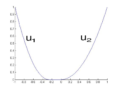
Figure 1. The plot of $u_{1}+u_{2}.$

Example 4.2.

Consider Problem (A) with $m=3$ and $f_{1}=f_{2}=1,f_{3}=\frac{1}{4}.$ The free boundary is shown in Figure 2. The boundary value $g$ is given by

$$g(x,y)=\left\{\begin{array}[]{lll}4-x^{2}&-2\leq x\leq+2\ {\&}\ y=-2,\\ 4-y^{2}&-2\leq y\leq+2\ {\&}\ x=-2,\\ \frac{4-x^{2}}{2}&-2\leq x\leq+2\ {\&}\ y=-x.\\ \end{array}\right.\hskip 7.22743pt$$

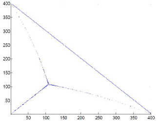
(a) The free boundaries

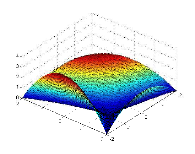
(b) $u_{1}+u_{2}+u_{3}$

Figure 2. The left picture shows the free boundaries of solutions. The right picture shows the surface of $u_{1}+u_{2}+u_{3}.$

Example 4.3.

Let $\Omega=[-1,1]\times[-1,1]$ and $m=4,f_{1}=8;f_{2}=6;f_{3}=2;f_{4}=1.$ The boundary values $\phi_{i},$ (i=1,2,3,4) are given as follows:

$$\phi_{1}=\left\{\begin{array}[]{lr}1-x^{2}&x\in[-1,1]\ {\&}\ y=1,\\ 0&\ \ \text{elsewhere.}\end{array}\right.\hskip 7.22743pt\phi_{2}=\left\{\begin{array}[]{lr}1-y^{2}&y\in[-1,1]\ {\&}\ x=1,\\ 0&\ \ \text{elsewhere.}\end{array}\right.$$

$$\phi_{3}=\left\{\begin{array}[]{lr}1-x^{2}&x\in[-1,1]\ {\&}\ y=-1,\\ 0&\ \ \text{elsewhere.}\end{array}\right.\hskip 7.22743pt\phi_{4}=\left\{\begin{array}[]{lr}1-y^{2}&y\in[-1,1]\ {\&}\ x=-1,\\ 0&\ \ \text{elsewhere.}\end{array}\right.$$

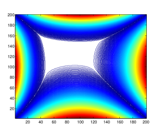
(a) contour

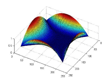
(b) $u_{1}+u_{2}+u_{3}+u_{4}$

Figure 3. The left picture shows the contours of solutions and zero set. The right picture shows the surface of $u_{1}+u_{2}+u_{3}+u_{4}.$

Example 4.4.

Let $\Omega$ be as in previous example and $m=4,f_{1}=0,f_{2}=|x^{2}-y^{2}|,f_{3}=8,f_{4}=|x+y|.$ The boundary conditions $\phi_{i},$ (i=1,2,3,4) are the same as in Example 4.3. The interfaces are shown in Figure 4.

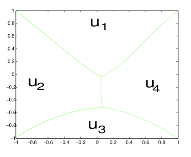
Figure 4. The picture shows the free boundaries of solutions of $u_{1},u_{2},u_{3}$ and $u_{4}.$

Now consider the following system of $m$ differential equations for $i=1,\cdots,m,$ as $\varepsilon\rightarrow 0,$

(4.3) $$\left\{\begin{array}[]{lll}-d_{i}\Delta u_{i}=\lambda u_{i}(1-u_{i})-\frac{1}{\varepsilon}u_{i}(x)\sum_{j\neq i}^{m}u_{j}^{2}(x)&\text{ in }\Omega,\\ u_{i}\geq 0&\text{ in }\Omega,\\ u_{i}(x)=\phi_{i}(x)&\text{ on }\partial\Omega.\\ \end{array}\right.$$

Example 4.5.

Let $\Omega=[0,1]\times[0,1],m=2,\lambda=1,d_{1}=1.5,d_{2}=1.$ The steady boundary values for $u(x,y,t),v(x,y,t)$ are defined by

$$\phi(x,0,t)=\left\{\begin{array}[]{ll}0.5-2.5x&0\leq x\leq 0.2,\\ 0&0.2\leq x\leq 1,\end{array}\right.\hskip 7.22743pt\phi(x,1,t)=\left\{\begin{array}[]{ll}0.5-\frac{5}{8}x&0\leq x\leq 0.2,\\ 0&0.8\leq x\leq 1,\\ \end{array}\right.$$

$$\phi(0,y,t)=0.5,\quad\quad\phi(1,y,t)=0,$$

and

$$\psi(x,0,t)=\left\{\begin{array}[]{ll}0&0\leq x\leq 0.2,\\ \frac{-1}{8}+\frac{5}{8}x&0.2\leq x\leq 1,\end{array}\right.\hskip 7.22743pt\psi(x,1,t)=\left\{\begin{array}[]{ll}0&0\leq x\leq 0.8,\\ -2+2.5x&0.8\leq x\leq 1,\\ \end{array}\right.$$

$$\psi(0,y,t)=0,\quad\quad\psi(1,y,t)=0.5,$$

Figure 5 shows boundary values of $u$ and $v.$ In Figure 6 the contours plot of solutions $u(x,y)$ and $v(x,y)$ are presented.

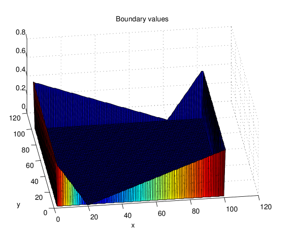
Figure 5. Boundary values for $u(x,y);$ left $v(x,y)$; in the right.

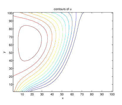
(a) contours of $u$

(b) contours of $v$

Figure 6. Contours of $u$ and $v.$

References

- [1] Bozorgnia, F. Numerical algorithm for spatial segregation of competitive systems. SIAM J. Sci. Comput. 31, 5 (2009), 3946–3958.
- [2] Conti, M., Terracini, S., and Verzini, G. Asymptotic estimates for the spatial segregation of competitive systems. Adv. Math. 195, 2 (2005), 524–560.
- [3] Conti, M., Terracini, S., and Verzini, G. A variational problem for the spatial segregation of reaction-diffusion systems. Indiana Univ. Math. J. 54, 3 (2005), 779–815.
- [4] Conti, M., Terracini, S., and Verzini, G. Uniqueness and least energy property for solutions to strongly competing systems. Interfaces Free Bound. 8, 4 (2006), 437–446.
- [5] Crooks, E. C. M., Dancer, E. N., and Hilhorst, D. Fast reaction limit and long time behavior for a competition-diffusion system with Dirichlet boundary conditions. Discrete Contin. Dyn. Syst. Ser. B 8, 1 (2007), 39–44 (electronic).
- [6] Crooks, E. C. M., Dancer, E. N., and Hilhorst, D. On long-time dynamics for competition-diffusion systems with inhomogeneous Dirichlet boundary conditions. Topol. Methods Nonlinear Anal. 30, 1 (2007), 1–36.
- [7] Crooks, E. C. M., Dancer, E. N., Hilhorst, D., Mimura, M., and Ninomiya, H. Spatial segregation limit of a competition-diffusion system with Dirichlet boundary conditions. Nonlinear Anal. Real World Appl. 5, 4 (2004), 645–665.
- [8] Dancer, E. N., and Du, Y. H. Competing species equations with diffusion, large interactions, and jumping nonlinearities. J. Differential Equations 114, 2 (1994), 434–475.
- [9] Dancer, E. N., Hilhorst, D., Mimura, M., and Peletier, L. A. Spatial segregation limit of a competition-diffusion system. European J. Appl. Math. 10, 2 (1999), 97–115.
- [10] Dancer, E. N., and Zhang, Z. Dynamics of Lotka-Volterra competition systems with large interaction. J. Differential Equations 182, 2 (2002), 470–489.
- [11] Dancer, N. Competing species systems with diffusion and large interactions. Rend. Sem. Mat. Fis. Milano 65 (1995), 23–33 (1997).
- [12] Ei, S.-I., and Yanagida, E. Dynamics of interfaces in competition-diffusion systems. SIAM J. Appl. Math. 54, 5 (1994), 1355–1373.
- [13] Glowinski, R. Numerical methods for nonlinear variational problems. Springer Series in Computational Physics. Springer-Verlag, New York, 1984.
- [14] Squassina, M. On the long term spatial segregation for a competition-diffusion system. Asymptot. Anal. 57, 1-2 (2008), 83–103.
- [15] Squassina, M., and Zuccher, S. Numerical computations for the spatial segregation limit of some 2D competition-diffusion systems. Adv. Math. Sci. Appl. 18, 1 (2008), 83–104.
- [16] Struwe, M. Variational methods. Springer-Verlag, Berlin, 1990. Applications to nonlinear partial differential equations and Hamiltonian systems.
- [17] Weiss, G. S. Partial regularity for weak solutions of an elliptic free boundary problem. Comm. Partial Differential Equations 23, 3-4 (1998), 439–455.