Atmospheric PSF Interpolation for Weak Lensing
in Short Exposure Imaging Data

Abstract

A main science goal for the Large Synoptic Survey Telescope (LSST) is to measure the cosmic shear signal from weak lensing to extreme accuracy. One difficulty, however, is that with the short exposure time ($\simeq$15 seconds) proposed, the spatial variation of the Point Spread Function (PSF) shapes may be dominated by the atmosphere, in addition to optics errors. While optics errors mainly cause the PSF to vary on angular scales similar or larger than a single CCD sensor, the atmosphere generates stochastic structures on a wide range of angular scales. It thus becomes a challenge to infer the multi-scale, complex atmospheric PSF patterns by interpolating the sparsely sampled stars in the field. In this paper we present a new method, psfent, for interpolating the PSF shape parameters, based on reconstructing underlying shape parameter maps with a multi-scale maximum entropy algorithm. We demonstrate, using images from the LSST Photon Simulator, the performance of our approach relative to a 5th-order polynomial fit (representing the current standard) and a simple boxcar smoothing technique. Quantitatively, psfent predicts more accurate PSF models in all scenarios and the residual PSF errors are spatially less correlated. This improvement in PSF interpolation leads to a factor of 3.5 lower systematic errors in the shear power spectrum on scales smaller than $\sim 13^{\prime}$, compared to polynomial fitting. We estimate that with psfent and for stellar densities greater than $\simeq$1$/{\rm arcmin}^{2}$, the spurious shear correlation from PSF interpolation, after combining a complete 10-year dataset from LSST, is lower than the corresponding statistical uncertainties on the cosmic shear power spectrum, even under a conservative scenario.

1 Introduction

Gravitational lensing is the physical phenomenon where gravitational fields perturb the trajectory of light rays and therefore distort observed images (Schneider, 1992). In particular, the study of weak gravitational lensing involves measuring the statistical properties of an ensemble of distorted galaxy images (see e.g. Bartelmann & Schneider, 2001). Weak gravitational lensing is, in principle, one of the most powerful probes of dark matter and dark energy. By measuring, at different redshifts, the statistical distortion of background galaxies due to large scale cosmic structures – the “cosmic shear” – it is possible to place extremely tight constraints on the nature of dark energy (Jain & Seljak, 1997; Hu & Tegmark, 1999).

For observations to date, the accuracy of cosmic shear measurements has been mostly limited by the statistical variation of random galaxy shapes in the relatively small sky areas studied (Hoekstra et al., 2006; Semboloni et al., 2006; Hetterscheidt et al., 2006; Jarvis et al., 2006; Hetterscheidt et al., 2007; Benjamin et al., 2007; Schrabback et al., 2010). However, in future wide-field weak lensing surveys such as those planned with the Dark Energy Survey, LSST (Ivezic et al., 2008), and Euclid, extremely large datasets will greatly reduce the statistical errors, making these experiments systematics-limited.

A major source of systematic error in weak lensing comes from our incomplete knowledge of the PSF (Paulin-Henriksson et al., 2008). To account for the effect of the PSF on observed galaxy images, we need a model for it at every galaxy position; these models can be constrained by images of stars, which provide noisy estimates of the PSF shape that are more sparsely distributed than the galaxies. This is the “PSF interpolation problem”. In an earlier paper (Chang et al., 2012, hereafter C12), we quantified the spatial variation in the PSF shapes for a typical LSST 15-second exposure due to various physical effects, such as optics misalignments and atmospheric turbulence. We found that, although most of the PSF anisotropy due to instrumental effects varies smoothly over the field of view, the atmospheric turbulence can generate PSF spatial variation on a wide range of scales in these short exposures, with patterns that do not repeat over time. This poses a new PSF interpolation challenge quite different from that faced by previous studies, which relied on images with longer exposure times and/or contained large instrumental effects that dominate the errors.

These atmospheric features have been observed in short exposure ($\sim 10$ seconds) images by, for example, Wittman (2005) and Heymans et al. (2012, hereafter H12); in particular, H12 pointed out that such high frequency, turbulence-induced spatial PSF variations in single short exposures may lead to systematic errors in shear measurements at levels that cannot be ignored for future weak lensing surveys, were existing PSF interpolation techniques to be used.

In weak lensing analyses to date, the scheme used most often to interpolate the PSF between sparsely sampled stars has been to fit a low order two-dimensional spatial polynomial function to the stars’ shape parameters. Van Waerbeke et al. (2002) claimed that 2nd-order polynomials are sufficient to model the PSF anisotropy variation across a typical CCD sensor of size $\sim 10^{\prime}$, while other studies identified possible drawbacks of simple polynomial fitting and more sophisticated models have been suggested (e.g. Massey et al., 2002; Hoekstra, 2004; Van Waerbeke et al., 2005; Bergé et al., 2012). In general, being dominated by instrumental effects, which primarily generate large-scale, smooth features (Jarvis & Jain, 2004; Rhodes et al., 2007; Schrabback et al., 2010), the PSF anisotropy in long exposure data can be modelled reasonably well using low order interpolation methods, even though these patterns are only sparsely sampled by the relatively low density of stars in the field. However, for future synoptic wide-field surveys, such as LSST, where high cadence imaging is required, short exposures are inevitable. It is therefore important to re-examine the traditional PSF interpolation techniques, and develop new interpolation algorithms that are better suited for these data.

A deliberate effort is being made to study in detail the PSF patterns for LSST by carrying out end-to-end, photon-by-photon image simulations using the LSST Photon Simulator (PhoSim; Peterson et al., 2012, 2009; Connolly et al., 2010). The ray-tracing procedure includes models for the instrument response, telescope optics, and, most importantly for our purposes, the atmosphere. For a full description of the atmospheric model and quantitative comparison of the model against real data, we refer the reader to Peterson et al. (2012, hereafter P12). In this work, our focus is on studying the PSF interpolation problem, for which we require simulated data containing realistic atmospheric PSFs, with a range of strengths and spatial scales. The PhoSim images meet these criteria, as we demonstrated in P12 by comparing the relevant PSF characteristics in our simulated images with those seen by H12 in short exposure images taken by the MegaCam wide-field camera (1 degree²) on the Canada-France-Hawaii Telescope (CFHT). In this work we therefore test our new algorithm on PhoSim simulated images, for which we know the underlying PSF spatial variation.

Working with simulated images is vital for this particular task, since existing data that are suitable for our tests are very limited – our tests require wide-field, short-exposure images with high stellar densities, and taken under a wide range of atmospheric conditions. Simulations, with sufficiently high fidelity, allow us to test the absolute, as well as relative, accuracy of our algorithm in a more controlled fashion and with higher statistics. Our PhoSim approach can be seen as the next step beyond that taken by Bergé et al. (2012), who re-sampled PSF patterns observed in Subaru images. Here, we use PhoSim to generate large numbers of predicted LSST images with the relevant exposure time, 15 seconds – effectively amplifying the data taken with CFHT for a more rigorous testing.

The primary aim of this paper is to introduce a new PSF interpolation technique, and test it under controlled conditions. In both real and simulated PSF patterns we observe structure due to the atmosphere on many different angular scales: this motivates us to model the underlying anisotropy maps using a range of different-sized smoothing kernels. We infer the pixel values of these underlying maps from the noisy, sparsely sampled stellar shape data given a non-committal entropic prior. We quantitatively compare this new maximum entropy method with two other methods that represent the current standards, and investigate the performance of all three using high-fidelity simulations over a range of observing conditions.

The structure of this paper is as follows. In Section 2, we review briefly the relevant weak lensing theory and the PSF interpolation problem for weak lensing. We then describe, in Section 3, our new PSF interpolation method and give arguments for why it is well-suited for the particular problem at hand. In Section 4 we use simulated images to quantify the performance of our new method against two strawman PSF interpolation techniques. We also define the metrics that we use to quantify the performance of a given interpolation method. The results of this programme are presented in Section 5. We then discuss their implications in terms of the systematic errors in cosmic shear measurement for future weak lensing surveys and make suggestions for further improvements on psfent in Section 6. We conclude in Section 7.

2 Weak lensing and PSF interpolation

In the weak lensing regime, the effect of gravitational lensing is to add a small offset to the intrinsic ellipticity of each galaxy, where ellipticity is typically defined as a two-component complex “spinor”, $\boldsymbol{\varepsilon}=\varepsilon_{1}+i\varepsilon_{2}$ (see e.g. Schneider et al., 2002). The resulting observed ellipticity is a noisy but unbiased estimator of the applied shear. We then constructs certain statistics from these shear estimators to infer cosmology. One of the most popular statistics is the two-point ellipticity correlation function $\xi_{\pm}(\theta)$ for the ensemble of galaxies:

$$\xi_{\pm}(\theta)=\langle\varepsilon_{\rm t}(\theta_{0})\varepsilon_{\rm t}(\theta_{0}+\theta)\rangle\pm\langle\varepsilon_{\times}(\theta_{0})\varepsilon_{\times}(\theta_{0}+\theta)\rangle\;,$$ (1)

where the angle brackets indicate an average over galaxy pairs separated by $\theta$ (with one galaxy located at $\theta_{0}$) and the subscripts $t$ and $\times$ indicate an isotropised decomposition of $\boldsymbol{\varepsilon}$ along the line connecting a certain pair of galaxies. The shear correlation functions predicted from cosmology, compared with these observed galaxy ellipticity correlation functions, provide a route by which the cosmological parameters can be inferred.

The major challenge in a ground-based weak lensing analysis is to account for the instrumental and atmospheric PSF contribution to the observed galaxy shapes, such that these effects do not systematically contaminate the shear signal one wishes to measure. This involves “deconvolving” (approximately) the PSF from the galaxy images, where the PSF at each galaxy’s location is “interpolated” from the shapes of nearby stars.

A wide range of algorithms have been developed to model the shapes of the galaxies and stars, and to perform PSF deconvolution in the noisy data (see e.g. Heymans et al., 2006; Massey et al., 2007; Bridle et al., 2010; Kitching et al., 2012a, b, for a summary of the various methods). However, to date, the PSF interpolation problem has been taken to be of secondary importance, since the PSF ellipticity patterns in existing images appear to be largely instrumental in origin, somewhat repeatable, and well-modelled by smoothly-varying functions such as low-order polynomials. However, as we showed in P12 and C12, this may not be the case for future instruments such as LSST, which are specifically designed for weak lensing and have extremely tight requirements on the instrument-induced PSF anisotropy. In these circumstances, the atmospheric effects, which used to be subdominant to instrumental effects, now become one of the key components in determining the PSF shape and the PSF spatial variation. This implies that the PSF shapes may no longer be smoothly varying across the field and modelling the PSF variation with such assumptions may be problematic. In addition, since the atmospheric effects are more pronounced in short exposures, datasets such as LSST, which are composed of sets of multi-epoch short exposure images instead of one long exposure, may suffer more from the atmospheric effects in single exposures when constructing the PSF model from interpolation.

To illustrate this PSF interpolation challenge, we show in Figure 1 two single-component ($\varepsilon_{1}$), model-subtracted stellar ellipticity maps from 74-second exposure images taken with the CFHT MegaCam on a dense stellar field ($\sim 7$ stars per arcmin²). The two images used to construct Figure 1 were taken on the same patch of sky but in two different nights, which appear to have very different atmospheric conditions. The data in Figure 1 are taken from two of the catalogues used in H12, so we refer to their paper for further details of the dataset. Note that a 2nd-order polynomial was subtracted from the raw ellipticity measurements (as explained in H12) – this accounts for most of the instrumental PSF contribution, but may also have removed some large scale atmospheric features. These images demonstrate that PSF spatial patters contain the characteristic high frequency structures from the atmosphere, which is the main motivation for our new PSF interpolation method.

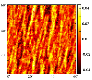
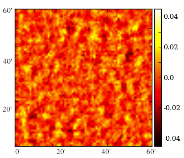
Figure 1: Examples of the residual PSF ellipticity ($\varepsilon_{1}$) patterns in $\sim$1 degree² sky regions, as observed in a dense stellar field with the CFHT MegaCam. The exposure time for these images is 74 seconds. As described in H12, a 2nd-order polynomial model has been fitted and subtracted from the raw stellar ellipticities to remove the optics contribution.

3 PSFent: a multi-scale inferential interpolation method

As seen in Figure 1, the atmospheric PSF anisotropy patterns can contain structure on a range of angular scales, with both patchy and striped features. This motivates us to look for flexible functions with which to model this spatial variability, which we can then fit to the sparsely sampled stellar PSF shape data in any given situation.

3.1 Interpolant model, and the likelihood function

Throughout this paper, we test the performance of our new interpolation method by interpolating two shape parameters: $\varepsilon_{1}$ and $\varepsilon_{2}$. In practice, a full weak lensing pipeline will require interpolation of several other shape parameters as well (e.g.PSF size, matrix elements of the shear polarisability in KSB-type methods (Kaiser et al., 1995) etc). We do not do a full analysis on these other parameters, but demonstrate in Appendix B that the our methodology is easily generalised to other parameters.

For the atmosphere-induced PSF, the two components of the ellipticity, $\varepsilon_{1}$ and $\varepsilon_{2}$, are expected to be independent from each other in each exposure, while both varying with similar amplitudes and spatial structures between different exposures. (We demonstrate this point with simulations in Appendix C.) This is because the physical mechanism that generates these ellipticity values – the refraction by turbulent cells – does not have a preferred direction, but does have a certain magnitude and spatial power spectrum dictated by the local atmospheric parameters (de Vries et al., 2007). As a result, we treat the two components of complex PSF ellipticity as independent fields with the same priors. These two fields, $\varepsilon_{1}(x,y)$ and $\varepsilon_{2}(x,y)$, are to be reconstructed from sparse, noisy, stellar shape data $\varepsilon^{\rm obs}_{1,k}$ and $\varepsilon^{\rm obs}_{2,k}$. Here, $k$ runs from 1 to the number of stars observed, $N_{star}$. Casting the PSF interpolation problem as an image restoration problem in this way allows us to properly take into account the observational errors on the measured star shapes, and propagate those errors into uncertainties on the interpolant. An iterative likelihood fit is performed: at each step, the two ellipticity components of each stellar image are predicted from the model underlying ellipticity fields and compared to the measured stellar ellipticities.

Both the predicted and observed data are inputs to the likelihood function. Under the assumption of uncorrelated Gaussian stellar shape uncertainties $\sigma_{k}$, this can be written for e.g.the first ellipticity component as the following probability distribution (PDF) for the data:

$${\rm Pr}(\boldsymbol{\varepsilon}^{\rm obs}_{1}| \boldsymbol{h}_{1})=\frac{1}{(2\pi)^{N_{star}/2}\prod_{k}\sigma_{1,k}}$$

$$\times\exp{\left(-\frac{1}{2}\sum_{k}\left[\frac{\varepsilon^{\rm obs}_{1,k}-\varepsilon_{1}(x_{k},y_{k};\boldsymbol{h}_{1})}{\sigma_{1,k}}\right]^{2}\right)},$$ (2)

and likewise for $\varepsilon_{2}$.

In Equation 2, $\boldsymbol{h}_{1}$ is a parameter vector that represents the model. It is the components of this parameter vector (and its companion $\boldsymbol{h}_{2}$ for $\varepsilon_{2}$) that we vary to fit the stellar shape data. We choose to parameterise the flexible interpolation functions $\varepsilon_{1}(x,y)$ and $\varepsilon_{2}(x,y)$ with pixelated grids on the sky. We compute the predicted ellipticity at the $k$th star position, $\varepsilon_{1}(x_{k},y_{k};\boldsymbol{h}_{1})$, by linear interpolation between the neighbouring pixels: we choose the pixel scale of each grid on our maps such that each pixel contains approximately 1 target point, on average, such that the linear interpolation choice does not affect the final prediction. For our test data, we fix the model map sizes at $80\times 80$ pixels for each ellipticity component.

Such free-form discretised functions like $\boldsymbol{h}_{1}$ and $\boldsymbol{h}_{2}$ have as many parameters to be inferred as there are pixels in the grids. However, we would like to impose some smoothness on these maps, such that structure on a range of angular scales can be predicted. We do this by constructing each map from a weighted sum of seven “hidden” maps, each convolved with a Gaussian “Intrinsic Correlation Function” (ICF) of a different angular scale: the result is known as the “visible” map. This procedure provides an efficient way of introducing smooth, correlated structure on a variety of angular scales. In our notation, $\boldsymbol{h}$ stands for “hidden.” We therefore have $7\times 80\times 80=44,800$ hidden pixel values to vary during the fit, for each ellipticity component. The convolutions with the ICF kernels reduce the effective number of free parameters, but even so many of these will still turn out not to be constrained by the few hundred data points in the field. The choice of prior PDF for the parameters in the $\boldsymbol{h}$ is therefore important.

3.2 The entropic prior PDF

We take the pixel values of the hidden images to be uncorrelated by construction, and assign a positive-negative entropic prior for them (Maisinger et al., 2004, hereafter MHL04). This has the effect of suppressing structure in the maps unless it is required by the data. In this way we give the method plenty of flexibility to fit the data well, but regularise to avoid over-fitting. Such a multi-scale maximum entropy method was first used by Weir (1992), and is implemented in the publicaly available MemSys4 code (Gull & Skilling, 1999). We illustrate the construction of a multi-scale ellipticity component map in Figure 2, showing how a range of different features on different angular scales can be modelled.

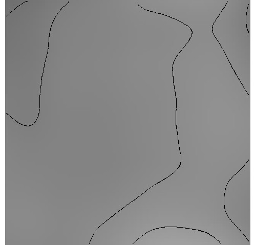
$\otimes$ $=$

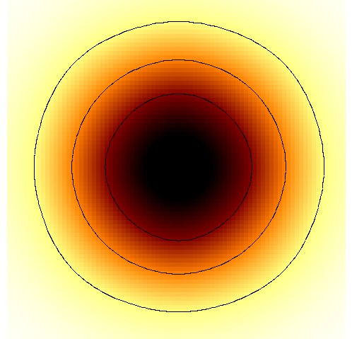
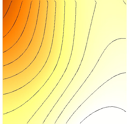
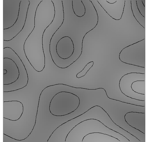
$\otimes$ $=$

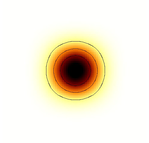
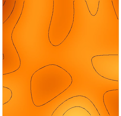
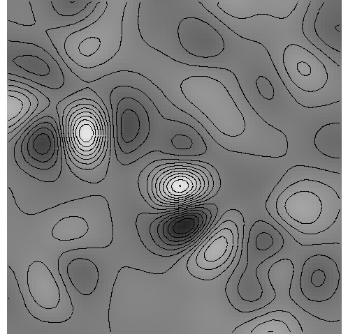
$\otimes$ $=$

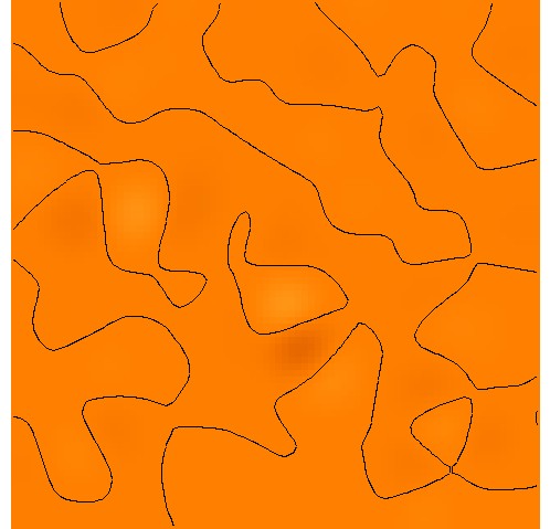
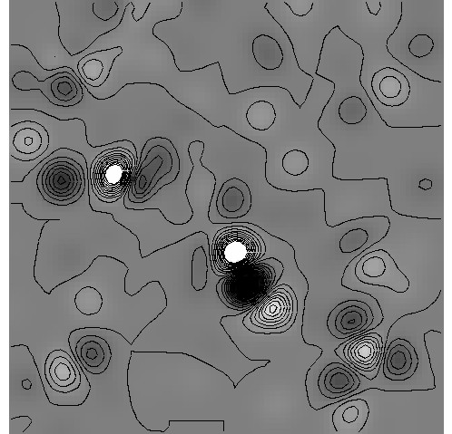
$\otimes$ $=$

$\otimes$ $=$

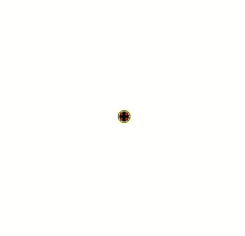
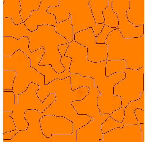
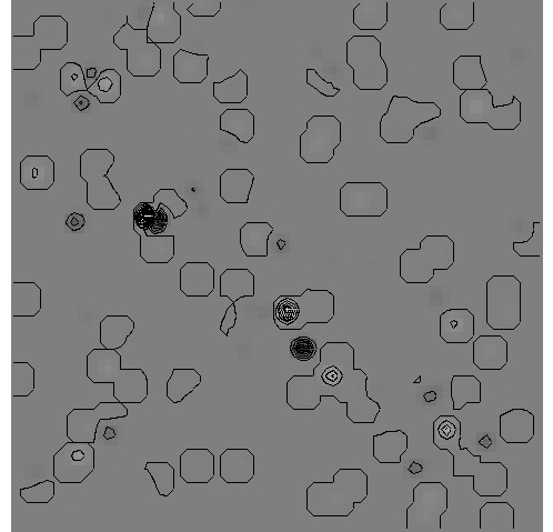
$\otimes$ $=$

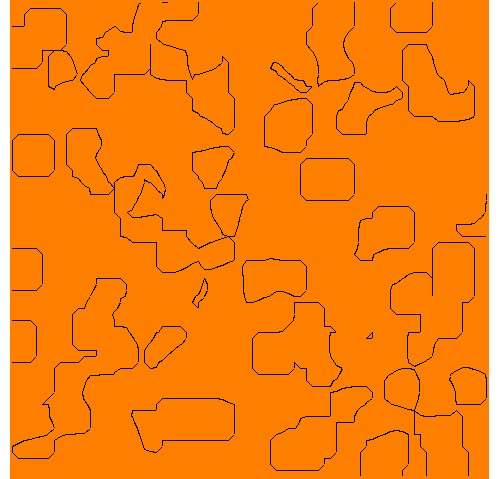
$\otimes$ $=$

$+$  

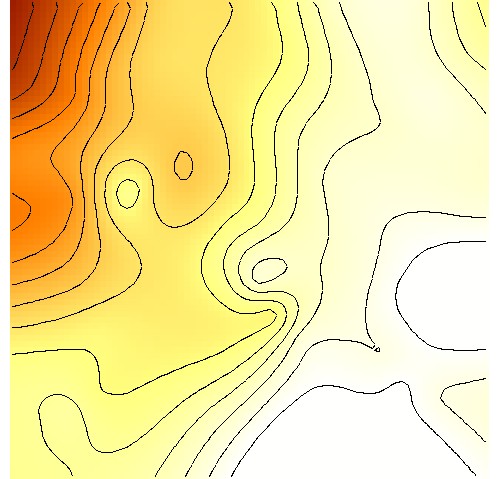
Figure 2: Illustrating the psfent multi-scale ellipticity map model. “Hidden” maps (left column, greyscale) are convolved with Gaussian kernels (ICFs) of exponentially-decreasing size (middle column) to make seven component “visible” maps (right, orange). These component maps are then weighted and summed to make the final model ellipticity map, which can be interpolated linearly onto any target position to predict the PSF shape there.

This model is similar in both essence and outcomes to one comprising a pixelated map and its “à trous” wavelet transform, as shown in some detail by MHL04. This wavelet transform can also be written as a set of convolutions; the implementation of MHL04 works well when making maps of the CMB temperature anisotropies, which also exhibit patchy features on a range of angular scales. Just like wavelet basis functions, the Gaussian ICFs we use have characteristic angular scales $w_{i}$ that increase approximately exponentially: the smallest is a single map pixel ($w_{0}=1$), while the largest is approximately $w_{6}=2^{6}=64$ pixels in size. The ICFs are normalised to unit volume.

The entropic prior PDF for a single hidden pixel value $h_{i}$ takes the following form

$${\rm Pr}(h_{i}|m_{i}) =\exp[{\alpha S(h_{i})}]\;,$$ (3)

$$S(h_{i}) =\psi_{i}-2m_{i}-h_{i}\log{\left(\frac{\psi_{i}-h_{i}}{2m_{i}}\right)}\;,$$ (4)

where $\psi_{i}=(h_{i}^{2}+4m_{i}^{2})^{1/2}$. This distribution peaks at zero and is symmetric. The “regularisation constant” $\alpha$ is a (nuisance) hyperparameter that parametrises the prior distribution. $\alpha$ is inferred from the data via the Bayesian evidence internally by MemSys4, and controls the final importance of the prior relative to the data. The “model” values $m_{i}$ (which we take to be constant over each hidden image) are also hyper-parameters, that determine the ease with which structure develops at each resolution scale: the smaller the value of $m_{i}$, the stronger the suppression of features at that scale.

3.3 Informing the prior

At this point we might ask whether we can inject any more information into the problem by choosing values of the $m_{i}$ to reflect the statistical properties of the simulated atmospheric PSF patterns. For a given pixel value, the entropic prior has approximate width $m\approx\sigma_{h}^{2}/2$, where $\sigma_{h}$ is the rms width of an approximating Gaussian (MHL04). This suggests that a possible algorithm for assigning the prior width at a particular resolution scale is to consider the variance of pixel histograms of low noise “true” multi-scale ICF hidden ellipticity maps at that scale.

To do this, we generate a special set of 100 simulated images with an ultra-high density of stars and low noise. The range of PSF patterns in these simulations is consistent with the simulations used in the main analyses and is described in more detail in Section 4.1. These unphysically dense star fields allow us to access the true PSF ellipticity pattern expected in the short exposures. The simulations are then run through psfent to be effectively “decomposed” into the 7 different scales, corresponding to the 7 ICFs. We generated one histogram for each of the 7 resolution scales that contain the pixel values ($\varepsilon_{1}$ and $\varepsilon_{2}$) in the hidden images for all 100 atmospheric PSF patterns on those scales. These histograms, as shown in Figure 3, are more peaked, and have broader wings, than a Gaussian distribution. The entropic prior PDF (in blue), while still imperfect, is a slightly better approximation to these distributions. We found the rms widths of the average histograms at the different scales increase from the smallest scale to the largest scale as: $m_{i}$=[0.0003, 0.0002, 0.0027, 0.0050, 0.0064, 0.0089, 0.0188]. There is very little power on the smallest two scales and nonlinear increase from the remaining middle to large scales. We adopt these numbers as the width for the entropic priors throughout the rest of the paper. We find that informing the priors in this way largely improves the accuracy of the PSF model constructed by psfent, compared to using flat, non-informative priors. We also find that using the default prior set in MemSys4 (which was optimised for CMB temperature map reconstruction) results in well-behaved PSF models, although quantitatively worse than the priors constructed from realistic simulations described above.

The standard deviation of the width of the grey histograms is approximately 30 – 40 $\%$ the mean width of the same histograms. This variation is due the variation in the atmospheric conditions in our simulations. For further optimisation of psfent, we could also use a narrower range of weather conditions and carry out the same process multiple times to derive priors as a function of different atmospheric parameters such as seeing and wind speed.

As an aside, we note that the process of assigning prior widths for the different angular scales plays a very similar role to the assignment of the range parameter in the covariance function of the Gaussian process at the heart of a Kriging interpolation (Bergé et al., 2012). The Kriging range parameter could also be derived by inspecting large numbers of high density simulated starfields, to capture the information present in the data-constrained atmospheric turbulence model in its most useful form.

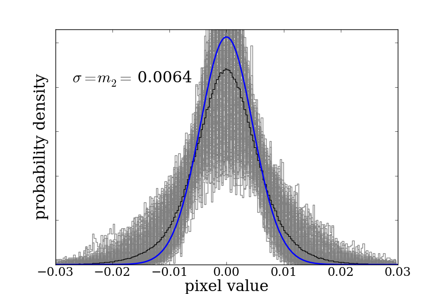
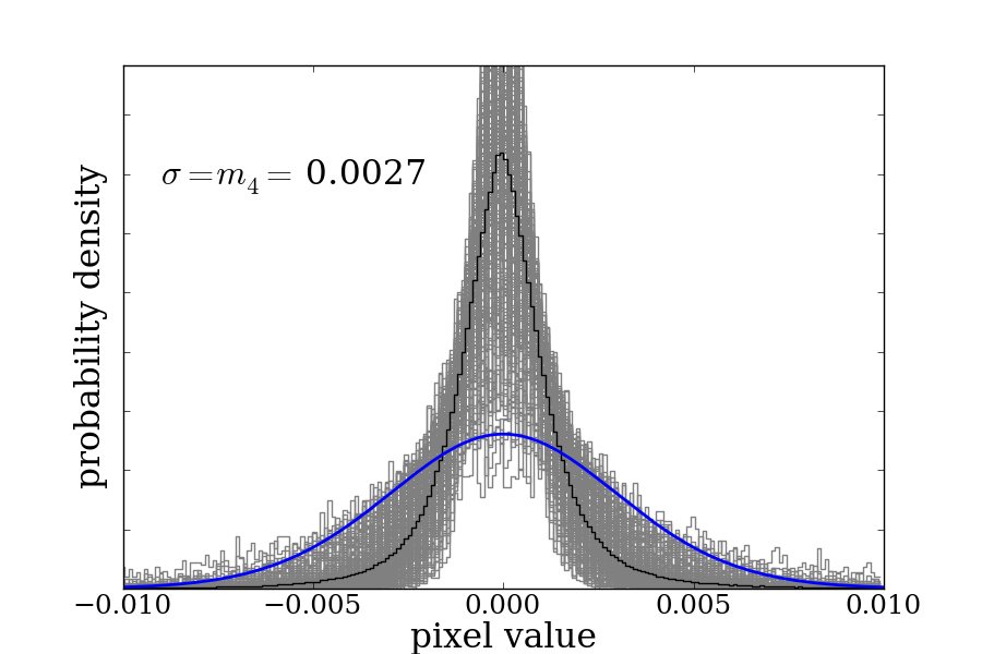
Figure 3: Setting the entropic prior PDF on the map pixels. We show here in blue the entropic prior PDF (Equation 4) for a single pixel value $h$ for two angular scales, 16 pixels (left) and 4 pixels (right). The grey curves are the pixel histograms of simulated ellipticity component maps at that scale, and the black curve is the average of those histograms. The entropic prior peaks at zero as required, and has slightly longer tails than a Gaussian. While the atmospheric PSF ellipticity map histograms have even longer tails and sharper peaks, especially on the smaller scales, by choosing the prior hyperparameter $m$ judiciously, the width of the histogram can be matched reasonably well. Note that the two plots have different scales on the x-axis – the histogram is much tighter for the smaller scales.

3.4 Estimating the posterior PDF

The posterior PDF, e.g.${\rm Pr}(\boldsymbol{h}_{j}|\{\varepsilon^{\rm obs}_{j}\})$, for the hidden pixel values given the data can be approximated by a multivariate Gaussian, centred at the maximum posterior point. The maximum posterior maps provide our best estimates for the PSF shape parameters at any target point in the field. Sample maps can be drawn from the posterior PDF in order to provide approximate uncertainties on these estimated PSF parameters. We find that 100 sample maps provide a sufficiently accurate standard deviation map, which we use for the uncertainties on the predicted PSF ellipticity estimates. This Gaussian approximation (including the maximum of the posterior, the covariance matrix of the parameters, and the associated evidence) is computed using the MemSys4 code, available on request from MaxEnt Data Consultants. Details of the implementation can be found in Gull & Skilling (1999).

4 Simulation and analysis

4.1 Simulations

As discussed in Section 1, since the existing datasets are insufficient for us to perform a systematic test with psfent, we depend on PhoSim to generate a large number of simulated images. We refer to P12, Peterson et al. (2009) and Connolly et al. (2010) for a complete description of PhoSim and in specific the details of the atmospheric model. Here, to facilitate comparison with parallel PSF interpolation studies, we provide a very brief overview of the PhoSim atmospheric model.

At the heart of the PhoSim atmospheric model is a system of seven-layer frozen Kolmogorov screens (Kolmogorov, 1992; Lane, R. G., 1992). These screens are constructed with density fluctuations obeying a full three-dimensional Kolmogorov energy spectrum of $E(k)\propto k^{-5/3}$, with values for the mean seeing, inner and outer turbulence scale assigned to each individual screen. All screens contain a wide range of turbulent structures, and these screens are carried by wind in different directions over the course of the exposure time. The distributions of wind speeds and atmosphere structure function parameters that PhoSim uses are based on observed data taken near the LSST site at Cerro Pachon, Chile. In P12, we demonstrated that with this atmospheric model, the simulations from PhoSim show sufficiently realistic atmosphere-induced PSF spatial variation for the purpose of weak lensing studies. Although PhoSim was designed to simulate images from LSST in particular, the atmospheric model in PhoSim generates PSF patterns qualitatively generic to most large aperture telescopes. The result of this study can thus be easily extended to estimate the performance of our PSF interpolation method on other instruments.

Finally, in this paper, we follow the convention in C12 and simulate only the best 50% of the images in terms of image quality, where the median PSF size is $\sim 0.7$" full-width-half-maximum (FWHM). This is based on the fact that in previous cosmic shear measurements, most of the cosmic shear information appear to come from these “good” images (Hoekstra et al., 2006). That is, although one may be using all of the images, the bad images will be weighted low and thus the errors made in the PSF interpolation will also not be contributing as much to the final results. The range of atmospheric parameters used in the this work is consistent with C12, which also allows us to make statements of the spurious shear correlation function in Section 6.1.

4.2 Testing programme

We use a mock stellar catalogue to generate realistic images of star fields. The catalogue is based on the model of Jurić et al. (2008), and contains a realistic population of stars in a typical LSST field with corresponding characteristics for each star. The average observed density of the population is $\simeq 1/{\rm arcmin}^{2}$, which corresponds to that expected at a galactic latitude of $|b|\sim 60$; the equatorial coordinates of the portion of the star catalogue used for this baseline simulated field was $(1.5,+0.2)$ degrees.

Two competing factors come into play in the PSF interpolation problem: (1) the complexity of the PSF patterns, and (2) the number of stars available for constructing a PSF model (or effectively, the galactic latitude). The more complex the PSF pattern, or the fewer stars available to interpolate, the more challenging it is to infer the PSF model from stars. The two effects are tested separately with the simulation and analysis pipeline described below.

We address (1) by generating 100 realisations of the atmospheric PSF patterns, and “observing” the mock star fields at these 100 different “epochs.” We generate these PSF realisations using the realistic distribution of atmospheric parameters described in P12. The median PSF size in our simulations is $\sim 0.66^{\prime\prime}$ – for LSST, this corresponds to approximately half of the exposures with the best image quality. Each atmosphere realisation creates a unique PSF pattern; simulating 100 independently corresponds to a low-cadence survey campaign where observations are well-separated in time.

To investigate (2), we do not actually simulate star fields at different galactic latitudes. Instead, we create an over-sampled stellar catalogue based on the same stellar population used for (1), so that our PhoSim input catalogue contains higher stellar density than an “average” field, while retaining the same signal to noise threshold in all “detected” star catalogs. We then down-sample at the detection catalogue level to achieve any desired stellar density used for interpolation – which can then be associated with a given galactic latitude. In this analysis, we consider stellar densities between the range 4 and 0.25 ${\rm arcmin}^{-2}$, which approximately covers the range of galactic latitudes $|b|>25$. As will be explained later, the stellar density quoted here is after a signal-to-noise ratio (SNR) cut, which eliminates very dim stars and noise peaks ($r>$23.5). In reality, harder cuts may be used to guarantee purity of the star sample.

For each of the above scenarios we generate one image containing only the expected stars at their given positions, and a second image containing an ultra-dense grid of bright stars ($\sim 50/{\rm arcmin}^{2}$) to sample the “true” PSF pattern. Noise corresponding to a sky background level of 22 mag/arcsec² was added to the star field images. All images were generated in the $r$ band for a single CCD sensor near the center of the LSST focal plane, which corresponds to a 13.6${}^{\prime}\times$13.6^′ field on the sky.

The suite of simulated images were analysed using the same pipeline, in which stars were first detected using the Source Extractor (Bertin & Arnouts, 1996) package, and then catalogued using the imcat software developed by Nick Kaiser. Shape estimation was performed using the imcat routine “getshapes”. We use the output “e[0]” and “e[1]” as our representative measures of ellipticity ($\varepsilon^{\rm obs}_{1,k}$ and $\varepsilon^{\rm obs}_{2,k}$ in Section 3) and retained stars measured with imcat parameter “$\nu$” larger than 25 (equivalent to a signal-to-noise cut $\sim$13). In the absence of uncertainty estimates on the ellipticity components, we propagate $\nu$ as the stars’ statistical weight.

psfent, together with two other PSF modelling methods, polynomial fitting and boxcar smoothing (details of our implementation of which are given in Appendix A), were then applied to the detected stars. From each method, the output was a list of predicted values of the PSF ellipticity at the ultra-dense grid positions of the bright stars in the “true PSF” image. These grid positions stand for background galaxy positions in a real lensing analysis. In this way we were able to compare the output catalogues directly with the true underlying ellipticity maps.

4.3 Performance metrics

To quantitatively evaluate the performance of the different PSF interpolation techniques, we employ two performance metrics in this paper. The first metric, $\sigma[\varepsilon_{\rm PSF}]$, is defined to be the root-mean-square of the PSF ellipticity model error:

$$\sigma[\varepsilon_{\rm PSF}]=\sqrt{\langle\delta\varepsilon^{2}_{1}\rangle+\langle\delta\varepsilon^{2}_{2}\rangle}\;.$$ (5)

where

$$\delta\varepsilon_{i}=\varepsilon_{i,\rm model}-\varepsilon_{i,\rm true}\;.$$ (6)

The second metric, ${\tilde{\sigma}_{\rm sys,PSF}}^{2}$, is defined as the average amplitude of the two-point correlation function of the PSF ellipticity model errors in the scales of interest:

$${\tilde{\sigma}_{\rm sys,PSF}}^{2}=\frac{1}{\theta_{\rm max}-\theta_{\rm min}}\int_{\theta_{\rm min}}^{\theta_{\rm max}}|\xi^{s,\rm PSF}_{+}(\theta)|d\theta\;,$$ (7)

where $\xi^{s,\rm PSF}_{+}(\theta)$ is the correlation function of $\delta\boldsymbol{\varepsilon}=\delta\varepsilon_{1}+i\delta\varepsilon_{2}$. The absolute value in the integrand prevents the anti-correlation regime canceling out some of the correlation signal. We use $\theta_{\rm min}=0.5^{\prime}$ and $\theta_{\rm max}=13^{\prime}$ in our single LSST CCD sensor ($13.6^{\prime}\times 13.6^{\prime}$) simulations. This range is chosen to sample the correlated PSF model errors on the full sensor while eliminating small scales far below the average stellar separation and large scales that come close to the boundaries.

Note that $\sigma[\varepsilon_{\rm PSF}]$ measures the level of the absolute errors in a certain PSF model, while ${\tilde{\sigma}_{\rm sys,PSF}}^{2}$ is a measure of the spatial correlation of the PSF model errors, in addition to their absolute levels. This motivates us to take the ratio of these two contributions and define an auxiliary metric $F_{\rm sys}$:

$$F_{\rm sys}=\frac{{\tilde{\sigma}_{\rm sys,PSF}}^{2}}{\sigma[\varepsilon_{\rm PSF}]^{2}}$$ (8)

$F_{\rm sys}$ is a relative measure of the how spatially-correlated the residual ellipticities are, independent of the absolute magnitude of the residual ellipticities. As seen in later sections, this figure facilitates our comparison of different PSF interpolation methods.

4.4 Scaling with number of exposures

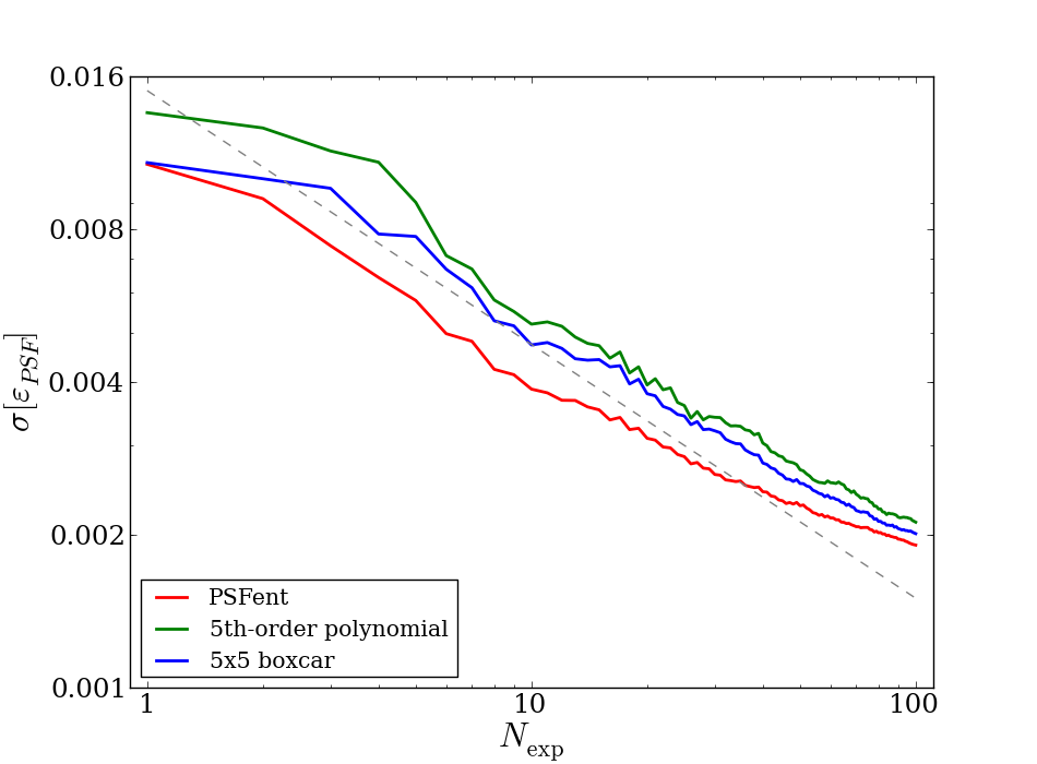
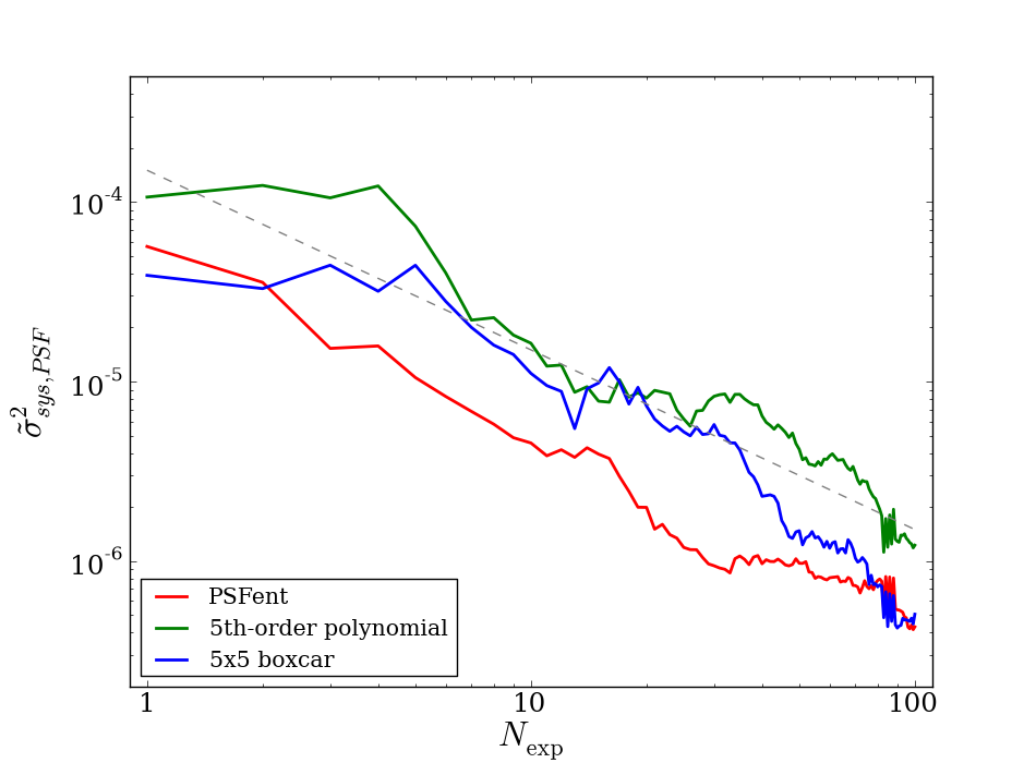
Figure 4: (a) $\sigma[\varepsilon_{\rm PSF}]$ and (b) ${\tilde{\sigma}_{\rm sys,PSF}}^{2}$ calculated as a function of the number of exposures combined (averaged), $N_{\rm exp}$. We show in both panels results for psfent (red), 5th-order polynomial fitting (green) and 5$\times$5 boxcar smoothing (blue). The grey dash line indicates the $1/\sqrt{N_{\rm exp}}$ and $1/N_{\rm exp}$ slope with arbitrary normalisation for (a) and (b) respectively. All three statistics in both plots roughly follow the $N_{\rm exp}$ scaling suggested by the grey lines.

In the main analysis in this paper (Section 5), we quantify the errors on the PSF ellipticity model for different interpolation techniques for a single LSST exposure. In reality, one can suppress the systematic errors that are independent between frames when properly combining multiple exposures. It is the final combined systematic error of all the data that impacts the cosmological constraints from weak lensing.

When the multiple exposures are far separated in time, the atmospheric conditions are different and one expects the PSF patterns to be independent. Similarly, the errors on the PSF model are also expected to be independent. This suggests that when averaging the ellipticity measurement of the same galaxy over $N_{\rm exp}$ exposures, the ellipticity errors from the atmosphere are expected to reduced as $1/\sqrt{N_{\rm exp}}$ (corresponding to $\sigma[\varepsilon_{\rm PSF}]$), and the correlation of these errors should drop by $1/N_{\rm exp}$ (corresponding to ${\tilde{\sigma}_{\rm sys,PSF}}^{2}$), or:

$$\sigma[\varepsilon_{\rm PSF}]\propto\frac{1}{\sqrt{N_{\rm exp}}}\;;$$ (9)

$$\sigma[\varepsilon_{\rm PSF}]\propto\frac{1}{N_{\rm exp}}\;.$$ (10)

This can be nicely demonstrated by performing the following test: we take the 100 realisations of simulated atmospheric PSF and average the PSF model prediction at each position over the first $N_{\rm exp}$ frames. $\sigma[\varepsilon_{\rm PSF}]$ and ${\tilde{\sigma}_{\rm sys,PSF}}^{2}$ is then calculated for the “average frame” and plotted against $N_{\rm exp}$ in Figure 4. The two statistics scale with $N_{\rm exp}$ as expected in Equations 9 and 10, which confirms that the errors produced by all three interpolation methods used in this paper are stochastic over different exposures.

We use the results in Figure 4 to support arguments later in Section 6.1, where we estimate the number of exposures needed to reach a certain level of PSF model accuracy.

5 Results

5.1 Variation with PSF pattern

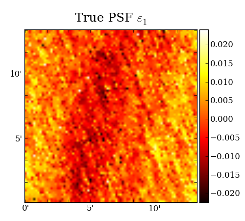
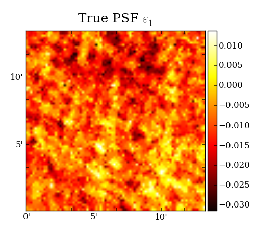
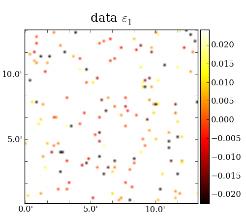
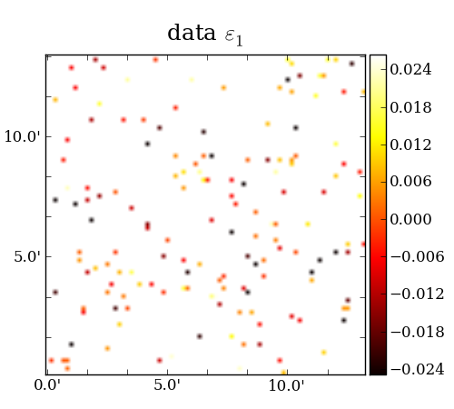
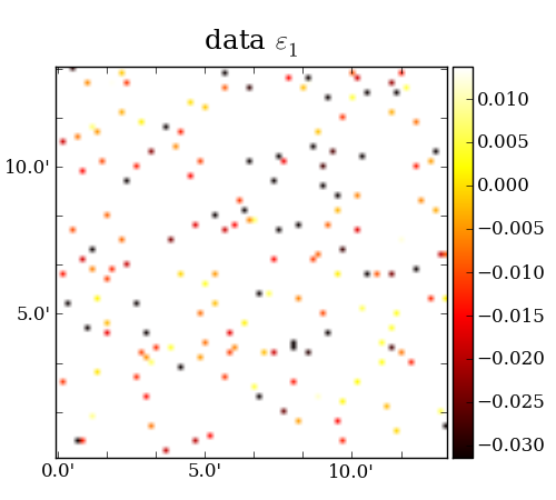
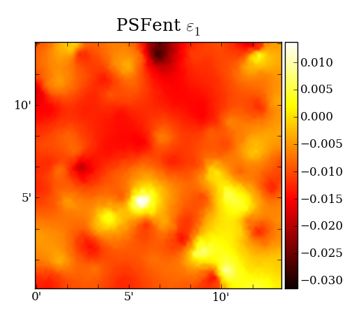
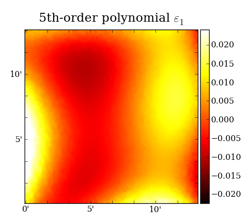
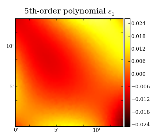
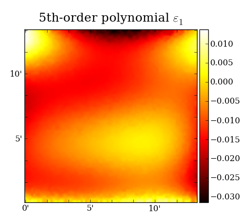
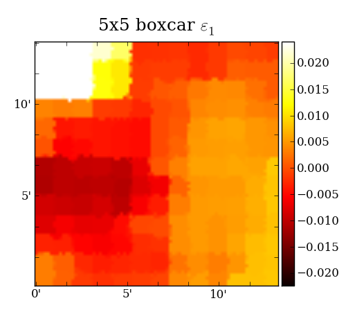
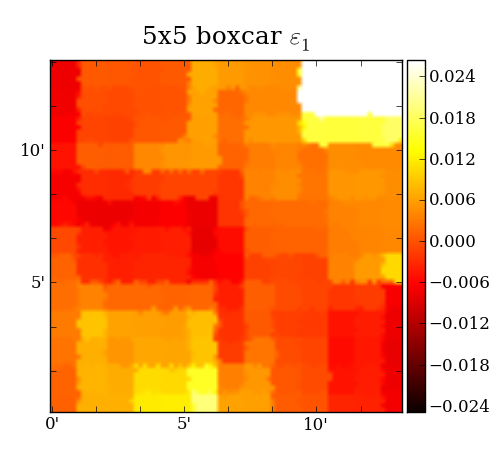
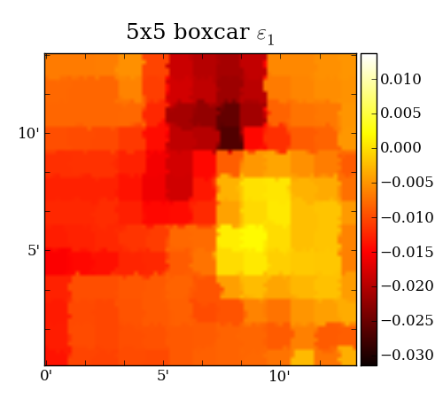
Figure 5: Illustration of the short exposure PSF interpolation problem, and the performance of different interpolation methods when we have very different PSF patterns. The three different realisations all have stellar density $\sim 1/{\rm arcmin}^{2}$. The maps in the first row show the “true” PSF ellipticity ($\epsilon_{1}$) field that we would like to reconstruct from the stellar data in the second row, the observed stellar ellipticities. The last three rows show model PSF ellipticity maps constructed with psfent, a 5th-order polynomial fit and a 5$\times$ 5-pixel boxcar smoothing, respectively.

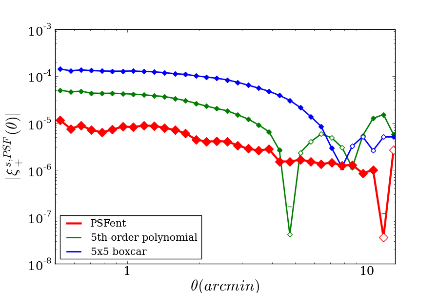
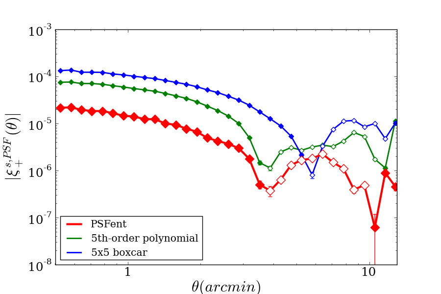
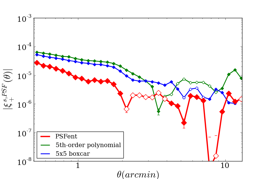
Figure 6: Absolute two-point correlation functions of the PSF ellipticity model errors for the three different PSF patterns in Figure 5. In each panel, we show results for psfent (red), 5th-order polynomial fitting (green) and 5$\times$5-pixel boxcar smoothing (blue). The hollowed labels indicate negative values.

The 100 atmospheric realisations in our simulation suite provide a wide range of PSF patterns. For example, three very different PSF patterns on a single LSST CCD sensor are shown in the top row of Figure 5, where the colours represent true PSF $\varepsilon_{1}$ values. We treat the $\varepsilon_{1}$ and $\varepsilon_{2}$ patterns as they were independent, as noted earlier, and only show $\varepsilon_{1}$ here.

We observe that the left column (a) contains a PSF pattern with some large-scale stripes that vary smoothly across the CCD sensor, with very fine ripples aligned at a direction different from the large stripes; the middle column (b) contains medium-size blobs without any preferred direction; finally, the right column (c) shows nearly equal strength of stripes in two nearly orthogonal directions, creating a grainy high-frequency pattern. When attempting to model these patterns at a typical galactic latitude of $|b|\sim 60$ (stellar density $\simeq 1/{\rm arcmin}^{2}$), the stars available to us for reconstructing these PSF patterns are shown in the second row on the same ellipticity colour scale. The last three rows of Figure 5 show the PSF model generated from three different PSF interpolation techniques in the following order: psfent, 5th-order polynomial fitting and $5\times 5$-pixel boxcar smoothing.

Visually, one can readily see the power of psfent in modelling the very different PSF patterns over the other two methods. In (a), all three methods failed to model the fine ripples, since they are much finer than the average stellar separations. They all do, however, manage to pick up the smooth “stripe” component. Both the polynomial and boxcar model in this case show bad behaviours on the edges of the field, due to the small number of ill-measured stars dominating the model. In (b), where the underlying PSF patterns consist of mainly medium scale “patches”, the Gaussian ICF used in psfent enables the model to capture these features nicely, which is not possible with a polynomial model. The boxcar model, on the other hand, is limited by the size of the filter, which in this case is slightly larger than the patches in the patterns. Finally in the right column (c), we show an example where the polynomial model becomes worse than even a simple boxcar smoothing. In this case the PSF pattern almost has no power on the large scales, causing the polynomial model to be entirely dominated by the noise.

In all the cases shown here, we can see the flexible multi-scale algorithm allows psfent to model structures on a large number of scales, and is well regulated by the prior construction thus less sensitive to noise.

The absolute correlation functions $|\xi_{+}^{s,\rm PSF}|$ for the three examples in Figure 5 are shown in Figure 6. In general, the model errors are more correlated on small scales due to the sparse sampling, and the limited resolution for all three modelling techniques. The shape of these correlation functions can be either smooth or oscillating. In particular, for polynomial models, the shape of $\xi_{+}^{s,\rm PSF}$ has some characteristic features: a transition from positive (correlation) to negative (anti-correlation) always appear at 3^′ – $4^{\prime}$. As discussed in H12, this is a result of both the modelling method and the true atmospheric PSF pattern.

Figure 7 shows, for the 100 different realisations of the atmosphere, the median behaviour of these ellipticity error correlation functions with the error bars indicating the standard deviation of the 100 curves divided by $\sqrt{100}$. The median $\sigma[\varepsilon_{\rm PSF}]$ and ${\tilde{\sigma}_{\rm sys,PSF}}^{2}$ values for these 100 atmospheric realisations are listed in Table 1. The final column $F_{\rm sys}$, as explained earlier, is a measure of the relative reduction in spatially-correlated residual ellipticity for the level of spatial correlation in the model errors independent of the absolute errors. Quantitatively, psfent provides $\sim 17\%$ improvement in the absolute ellipticity modelling error, or $\sigma[\varepsilon_{\rm PSF}]$, over the 5th-order polynomial and $\sim 22\%$ improvement over the boxcar smoothing model. For the correlation of these errors, or ${\tilde{\sigma}_{\rm sys,PSF}}^{2}$, psfent performs $\sim 3.5$ times better than the polynomial model and $\sim 7$ times better than boxcar smoothing. The corresponding $F_{\rm sys}$ values suggest that the model errors from psfent is $\sim 2.5$ times less correlated than that from polynomial models and $\sim 4.2$ times less correlated than that from boxcar models. Notice that the main power in psfent lies not in the absolute reduction of the model errors, but in the fact that the flexible free-form model creates makes errors less correlated in space, which is an important property for measurements like cosmic shear, where the main signal is embedded in the spatial correlation of galaxy shapes.

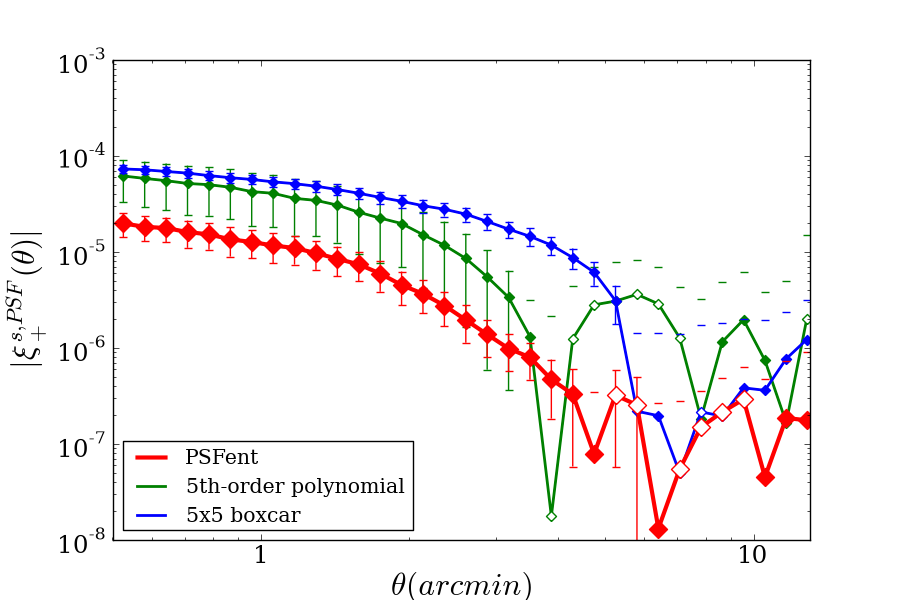
Figure 7: Median correlation function of the PSF ellipticity model errors of 100 different PSF patterns, at the “typical” stellar density of $1/{\rm arcmin}^{2}$. The results are shown for psfent (red), 5th-order polynomial fitting (green) and 5$\times$5 boxcar filtering (blue). The error bars indicate the rms spread in the 100 exposures divided by $\sqrt{100}$. Hollowed labels indicate negative values.

	$\sigma[\varepsilon_{\rm PSF}]$	${\tilde{\sigma}_{\rm sys,PSF}}^{2}$	$F_{\rm sys}$
psfent	7.41$\times 10^{-3}$	2.41$\times 10^{-6}$	4.39$\times 10^{-2}$
Polynomial	8.93 $\times 10^{-3}$	8.67$\times 10^{-6}$	10.87$\times 10^{-2}$
Boxcar	9.51 $\times 10^{-3}$	16.77$\times 10^{-6}$	18.54$\times 10^{-2}$

Table 1: Median metric $\sigma[\varepsilon_{\rm PSF}]$ and ${\tilde{\sigma}_{\rm sys,PSF}}^{2}$ for the three PSF interpolation techniques for 100 different PSF patterns sampled at the nominal stellar density of $1/{\rm arcmin}^{2}$. The final column $F_{\rm sys}$ is a measure of the level of the spatial correlations in the PSF model errors, independent of the absolute errors.

5.2 Variation with stellar density

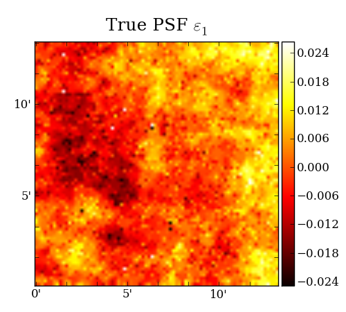
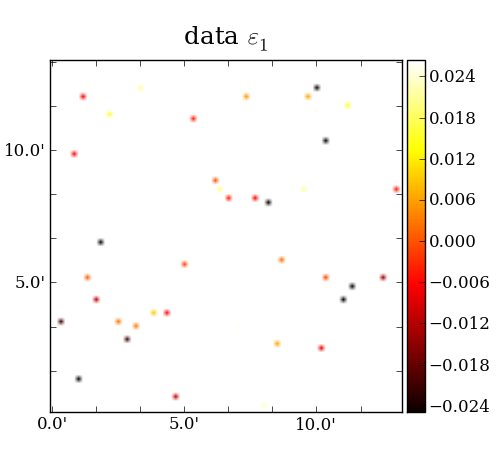
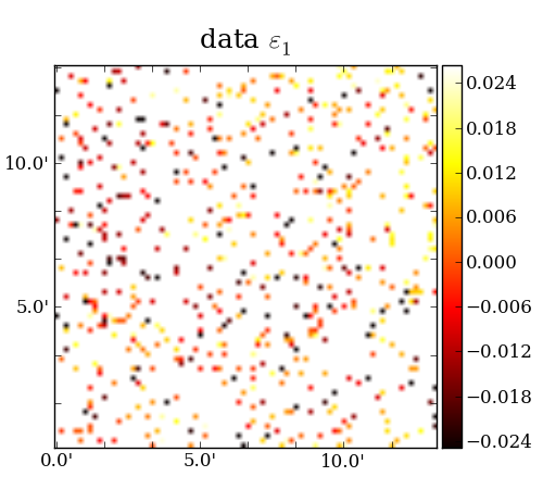
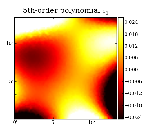
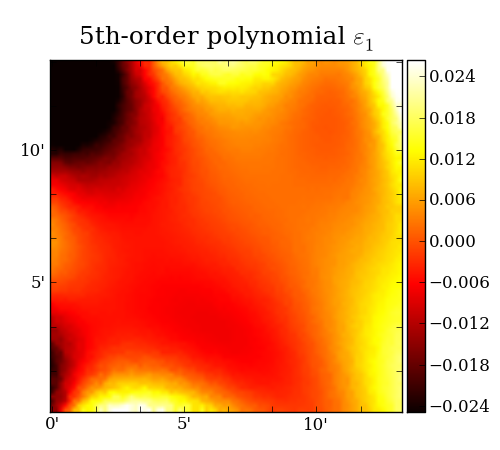
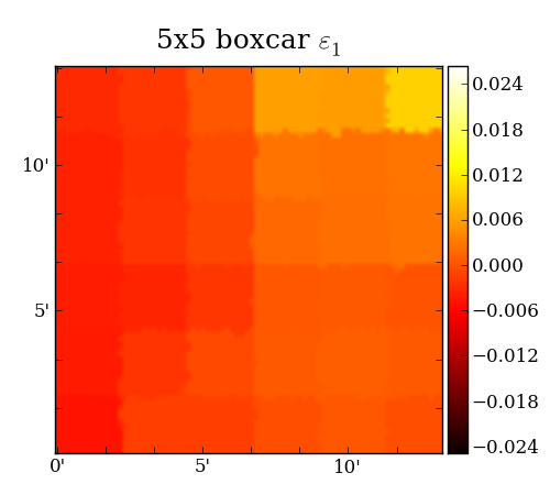
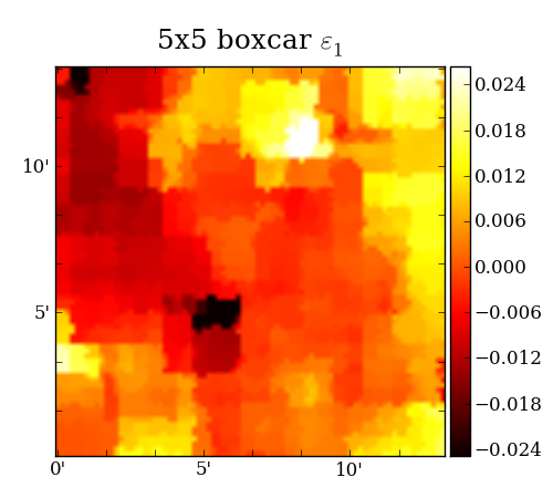
Figure 8: Illustration of the single short exposure PSF interpolation problem, and the performance of different interpolation methods as a function of stellar density. See the caption of Figure 5 for the description of the maps in the five rows; the different columns correspond to the same atmospheric PSF pattern (Figure 5 (b)), but sampled by stars with densities of 0.25 (a), 1 (b) and 4 (c) ${\rm/arcmin}^{2}$, as shown in the second row.

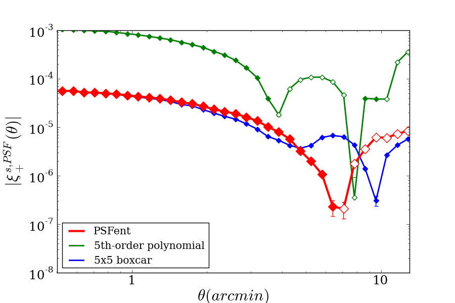
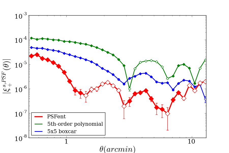
Figure 9: Absolute two point correlation functions of the PSF ellipticity model errors for different stellar densities: (a) 0.25, (b) 1 and (c) 4 ${\rm/arcmin}^{2}$. The three cases have the same underlying PSF pattern but are sampled at different rates. In each panel, we show results for psfent (red), 5th-order polynomial fitting green) and 5$\times$5 boxcar smoothing (blue). The hollowed labels indicate negative values.

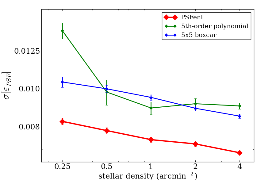
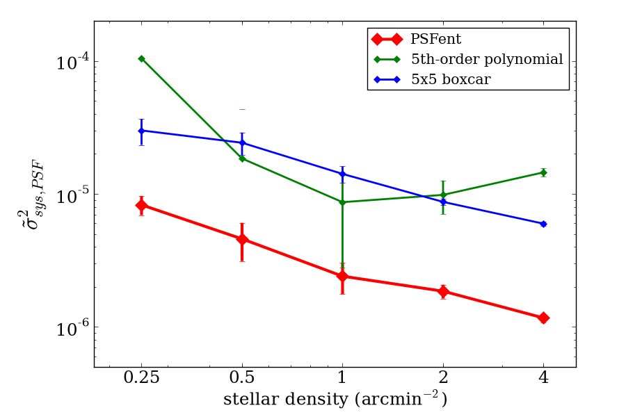
Figure 10: Median values for 100 PSF patterns for the two statistics: (a) $\sigma[\varepsilon_{\rm PSF}]$ and (b) ${\tilde{\sigma}_{\rm sys,PSF}}^{2}$ over a range of stellar densities. The error bars show the interquartile range divided by $\sqrt{100}$. We show in each panel results for psfent (red), 5th-order polynomial fitting (green) and 5$\times$5 boxcar smoothing (blue). In both statistics, psfent performs consistently better than the other two techniques.

Having examined the performance of the three PSF interpolation methods on a “typical” field, we would now like to understand how the three PSF interpolation schemes are affected by the available density of stars (we explore the range from 0.25 to 4 stars per arcmin² for a complete sample of realistic stellar distributions). This test is especially important for images at high galactic latitude, where stars are very sparse. The ability to reconstruct the PSF variation at these fields may increase the effective area of a survey and therefore its statistical power. Figure 8 shows, for the PSF pattern in Figure 5 (b), how the PSF model improves, for the three interpolation methods, as the stellar density increases. Figure 9 shows how the residual ellipticity correlation in each case changes accordingly.

Figure 8 visually illustrates one example of how the three different interpolation methods respond to the increased available stellar data points. We observe that the polynomial models appear to be particularly ill behaved when the available stars are under-dense (a) and over-dense (c). This is an example of imposing an improper prior assumption about the PSF pattern while ignoring the data. In contrast, the simple boxcar smoothing technique works in the opposite direction, where the model is purely driven by data with essentially no assumption on the expected PSF patterns. As a result, the models are just reflecting the available data, where we get a model with no structure in the under-dense case (a), and a model with lots of small scale structure in the over-dense case (c). psfent is effectively a more sophisticated version of the boxcar smoothing with informative priors and multiple structure scales. The change from (a) to (c) for the psfent model is qualitatively similar to the boxcar smoothing, as it is primarily dictated by data. But when data is insufficient, as in (a), psfent does not generate entirely flat models like boxcar smoothing, rather, we can see traces of the psfent priors creating some structure in the PSF model. When the stellar data is abundant (c), psfent lets data take over to drive the fit and only makes sure that the model stays in a physically reasonable range as specified by the priors. Figure 9 confirms the above observation more quantitatively.

In Figure 10, we show for our 100 different atmosphere realisations the median $\sigma[\varepsilon_{\rm PSF}]$ and ${\tilde{\sigma}_{\rm sys,PSF}}^{2}$ statistics as a function of stellar density. In all stellar densities, psfent consistently performs $\sim 20\%$ better in $\sigma[\varepsilon_{\rm PSF}]$ and 3–10 times better in ${\tilde{\sigma}_{\rm sys,PSF}}^{2}$ compared to boxcar smoothing and polynomial fitting.

The two statistics show similar trends in general. As we explained earlier, for psfent and boxcar smoothing, since the model is primarily driven by data, the model improves monotonically as more data becomes available. The 20% and nearly 4-times improvement of psfent in $\sigma[\varepsilon_{\rm PSF}]$ and ${\tilde{\sigma}_{\rm sys,PSF}}^{2}$ respectively compared to boxcar smoothing mainly comes from psfent’s ability to capture multi-scale structures and regulate the model using priors so that noise does not get amplified. A fixed order polynomial function, on the other hand, when optimised for a certain stellar density (1$/\rm arcmin^{2}$), over-fits (Figure 8 (c)) or under-fits (Figure 8 (a)) data when the stellar density varies, which results in a local minimum in the two green curves. The polynomial model, when optimised, is a reasonably good description of the smooth variation in the large-scale PSF patterns, but still fails to capture the small-scale structures, which explains why psfent still performs better in that case.

Although we emphasise the improvement of psfent over the other two methods, it is important to note at this point that the main improvement here is not from the specific type of functional form (or un-parametrised model) one uses, but rather, the use of either realistic simulations or calibration data to inform the prior PDFs for the flexible model parameters. We chose pixelated maps for use in psfent because we learned from simulations that the PSF patterns are complicated and requiring a very flexible model. One can imagine, for example, an alternative method with the same spirit, where a basis of high-order polynomials are used to reconstruct the PSF variations with coefficients constrained by priors derived from simulations.

6 Discussion

6.1 Implications of $\sigma[\varepsilon_{\rm PSF}]$ and ${\tilde{\sigma}_{\rm sys,PSF}}^{2}$ on shear systematics

To project the improvement on PSF interpolation from psfent onto the improvement in weak lensing shear measurements for a LSST-like survey, we return to Table 1 and discuss the implications of the $\sigma[\varepsilon_{\rm PSF}]$ and ${\tilde{\sigma}_{\rm sys,PSF}}^{2}$ values under the nominal stellar density of 1$/{\rm arcmin}^{2}$.

According to Amara & Réfrégier (2008, hereafter AR08), for future stage IV ground-based weak lensing surveys (Albrecht et al., 2006) not to be systematics-limited, one can set limits on the allowed systematic errors on the spurious shear power spectrum. Paulin-Henriksson et al. (2008) extended from AR08 and estimated that the allowed errors on determining the PSF ellipticity corresponding to those limits on spurious shear power spectrum is:

$$\sigma[\varepsilon_{\rm PSF}]\leq 10^{-3}$$ (11)

Combining the first column in Table 1 and Equation 9, we can derive the number of exposures needed for each of the interpolation methods to achieve Equation 11 as listed in Table 2. Also listed is the corresponding operation time for LSST, where we have adapted the assumptions in C12 and assumed two different scenarios – “optimistic” ($N_{\rm exp}=368$) and “pessimistic” ($N_{\rm exp}=184$), where a total of $N_{\rm exp}$ single 15-second exposures are combined in the final 10-year dataset for cosmic shear measurements.

	$N_{\rm exp}$	operation time (years)
		optimistic	pessimistic
psfent	55	1.50	2.99
Polynomial	80	2.17	4.35
Boxcar	90	2.45	4.89

Table 2: Number of exposures required for the PSF ellipticity measurement accuracy to meet Equation 11 for the three PSF interpolation methods under nominal conditions. Also listed are the corresponding expected time span these exposures can be obtained by LSST in the optimistic and pessimistic scenarios.

	$N_{\rm exp}$	operation time (years)
		optimistic	pessimistic
psfent	105	2.86	5.72
Polynomial	368	10.0	20.0
Boxcar	710	19.34	38.7

Table 3: Number of exposures required for the PSF ellipticity measurement accuracy to meet the target value set by AR08 and C12 for the three PSF interpolation methods under nominal conditions. Also listed are the corresponding expected time span these exposures can be obtained by LSST in the optimistic and pessimistic scenarios.

However, we note that Equation 11 is a rather simplistic estimation that does not account properly for the correlation properties of these errors and the spurious shear arising from a realistic PSF correction pipeline. An alternative and more realistic approach to interpret the results from our study in terms of shear measurements is to turn to C12, where we looked at the additive spurious shear correlation function by actually measuring these levels on high fidelity simulations. We concluded in C12 that the polynomial PSF model generates spurious shear correlation approximately at the level required by AR08 in the optimistic case and 2 times too high in the pessimistic case. Since psfent provides a $\sim 3.5$ times improvement in the PSF error correlation over polynomial models (Table 1 second column), we can expect it to also lower the spurious shear power spectrum by a factor of $\sim 3.5$ if all the spurious shear is due to PSF interpolation errors. This brings the level of spurious shear power spectrum 3.5 (optimistic) and 1.75 (pessimistic) times lower than the target level. Combined with Equation 10, we summarise in Table 3 the results in terms of the number of exposures and survey time needed to achieve the target value set in AR08.

On the other hand, if one considers that there are shear measurement algorithm errors that have not been accounted for in C12, then the situation could be worse. Assume, for example, these unaccounted algorithm errors take up to $50\%$ the allowed systematic errors set by AR08, the improvement in psfent then results in a spurious shear power spectrum about 1.3 times lower (optimistic) and 1.1 times higher (pessimistic) than the target level. In that case, even psfent will be a marginal failure in the pessimistic scenario.

6.2 Correlating galaxies across exposures

Correlating galaxy ellipticities in different exposures has been one of the proposed solutions to the problem of stochastic atmospheric PSF correlations (Jain et al., 2006). This, however, comes at the price of decreasing the statistical power of the survey. Exploring the tradeoff between statistical and systematic PSF interpolation errors using this technique is not the main focus of this paper. Here, we have effectively assumed a LensFit-style (Miller et al., 2007) analysis, where the PSF ellipticity map is estimated for each exposure, the galaxy images deconvolved, and the ellipticity estimates simply averaged. This assumption is justified by the behaviour of the residual PSF ellipticity correlation function with increasing $N_{\rm exp}$ as we have shown. We presume that when correlating between different exposures, it will still be beneficial to start with a more accurately-interpolated PSF model.

6.3 Computational cost

On a standard 64-bit 2$\times$2.2 GHz processor, psfent takes on average $\sim$13.0 seconds per LSST CCD sensor per pair of shape parameters ($\varepsilon_{1},\varepsilon_{2}$). Adding error estimation (sampling from the posterior cloud) adds an extra $\sim$9 sec of run time. This is about an order of magnitude slower than the two other techniques we investigated. For more complicated shape parametrisation the runtime would increase linearly with the number of parameters, and also with the number of images analysed. For example, if psfent were to be used for in the LSST data processing pipeline, the PSF model in each exposure on the $\sim$200 CCD sensors would need to be calculated in $\sim$ 19 seconds (15-second exposure + 2-second readout + 2-second shutter open/close). This demands $\sim$200 computers running for the PSF reconstruction alone. Though large, these numbers are not outrageous considering the expected decrease in unit cost for computers over the next decade and the possibility of further accelerating the code via hardware parallelisation such as GPUs.

In the meantime, we recommend that the current code can be used for smaller scale datasets when extremely accurately interpolated PSF maps are vital for the specific science goal. As well as weak lensing, these might include reconstructing the detailed structures of complex objects, and precision photometry of faint objects.

7 Conclusions

In this paper we have introduced a new PSF interpolation method, psfent, based on a multi-scale maximum-entropy image reconstruction code. The problem we set out to solve is reconstructing the multi-scale spatial variations of PSF shapes, due to atmospheric turbulence, in short exposure images, from sparsely distributed, noisily measured stars – a potential problem for future weak lensing surveys such as LSST.

Our analysis of simulated data allows us to draw the following conclusions:

• Compared with two other PSF interpolation methods, one of which is commonly used in current data analyses, psfent provides more accurately interpolated PSF shapes: the absolute residual ellipticities improve $\sim 20\%$ while the correlated residual ellipticities are a factor 3 –10 smaller than the other two methods, over a wide range of different PSF patterns and stellar densities.

• When combining multi-epoch datasets, the interpolation errors due to the atmosphere are stochastic, decreasing with the number of exposures taken as $1/\sqrt{N_{\rm exp}}$. The correlation function amplitude decreases as $1/N_{\rm exp}$.

• The improvement in PSF modelling from psfent suppresses the spurious shear in cosmic shear measurements. Combining previous studies from realistic simulations and the results in this work, we estimate that systematic errors due to PSF interpolation for LSST will be 3.5 (optimistic) and 1.75 (pessimistic) times lower than the statistical errors.

• Taking into account other algorithm errors, however, the improvement from psfent may not be sufficient to bring the systematic errors down to the target level in the most pessimistic scenario.

While it may still become a practical solution even for large datasets such as LSST, the relatively high computational cost of powerful algorithms like psfent should motivate the development of faster inference methods. The paper by Bergé et al. (2012) appeared as we were completing this study: their results are complementary to those presented here, in that they investigate the PSF interpolation problem on larger scales, using re-sampled real Subaru data that is less dominated by the atmosphere. It would be very interesting to apply their Kriging technique to our simulated data, and compare performance in terms of accuracy and speed. Like Bergé et al. (2012), we have demonstrated the benefits of using very flexible models, but also the use of methods both inspired and constrained by realistic simulations. Injecting statistical information about the atmospheric PSF anisotropy into interpolation methods appears to be a fruitful approach.

All the simulated data used in this paper is freely available at the following website: http://www.slac.stanford.edu/~chihway/psfent/.

Appendix A Other modelling methods

A.1 Polynomial fitting

As discussed in Section 2, in most current weak lensing pipelines, the PSF spatial variation is assumed to be smoothly varying on scaled comparable to the field and can thus be modelled with some low order polynomial functions. We have shown that PSF patterns from short exposures, however, display higher frequency spatial variations that require higher order fits. As a result, we have examined polynomials of order 2 to 5 as PSF models and found that 2nd-order models are insufficient in representing the PSF variations; 3rd-order models are usually sufficient, but occasionally an even higher order model is needed. We choose to use 5th-order models in our main analyses, but have confirmed that in most cases, the results are identical to 3rd-order fits. We minimise the effective $\chi^{2}$:

$$\chi^{2}=\sum w_{\varepsilon}^{2}(\varepsilon^{model.j}_{i}(\boldsymbol{p};x,y)-\varepsilon_{i})^{2},\;i=1,2\;,$$ (12)

where $\varepsilon^{model,j}_{i}(\boldsymbol{p};x,y)$ is a two dimensional, $j$th order polynomial function of $(x,y)$, $\boldsymbol{p}$ are the fitting parameters and we use the signal-to-noise ratio of each star as $w_{\varepsilon}$.

A.2 Boxcar smoothing

Alternatively, we examine the approach of modelling the PSF by directly smoothing the stellar ellipticities with a boxcar filter. In this approach, stars need to first be binned into large pixels, where we assign a weighted average ellipticity to each pixel $(j_{1},j_{2})$, defined:

$$\overline{\varepsilon^{j_{1}j_{2}}_{i}}=\sum_{pixel\;(j_{1},j_{2})}W_{\varepsilon}\varepsilon_{i}\;,\;\;i=1,2\;.$$

The size of the pixels are determined by the number of stars – we pixilate the image so that in each pixel contains approximately 1 star. A boxcar filter of size $m\times m$ pixels is then applied to the large pixel grid so that the ellipticity of pixel $(j_{1},j_{2})$ is replaced by the average ellipticity of the neighbouring $(m^{2}-1)$ pixels:

$$\varepsilon^{model,j_{1}j_{2}}_{i}= \frac{1}{m^{2}-1}((\sum_{a=-m^{\prime}}^{m^{\prime}}\sum_{b=-m^{\prime}}^{m^{\prime}}\overline{\varepsilon^{(j_{1}+a)(j_{2}+b)}_{i}})-\overline{\varepsilon^{j_{1}j_{2}}_{i}})\;;$$

$$m^{\prime}= \frac{m-1}{2},\;i=1,2\;.$$

The original coordinates are then recovered so that the modelled PSF ellipticities of all points falling in pixel $(j_{1},j_{2})$ will be $\varepsilon^{model,j_{1}j_{2}}$

Appendix B PSFENT with other shape parameters

It had been shown in H12 that due to atmospheric distortion, the size of the PSF varies on spatial frequencies similar to that of $\varepsilon_{1}$ and $\varepsilon_{2}$. This suggests that with the same procedure described in Section 4, we could use psfent to interpolate the PSF size, and by extension other shape parameters. We demonstrate below our results of interpolating the shape parameter “FWHM_WORLD” output from Source Extractor (which is an estimate of the PSF FWHM size in arcseconds) with the three interpolation methods used in Section 5.

First we derive the appropriate priors ($m_{i}$ values) for FWHM_WORLD from the “true” PSF maps. We have $m_{i}$=[0.0001, 0.0002, 0.0026, 0.0055, 0.0079, 0.0100, 0.0206] for FWHM_WORLD. The set of priors for the FWHM_WORLD variation appear to follow the same trend as that of $\varepsilon_{1}$ and $\varepsilon_{2}$, while putting slightly more power on the larger scales. This can also be observed qualitatively in Figure 11, where we show the equivalent of Figure 5 (b), with the interpolant being the PSF size, $R$ (or FWHM_WORLD), instead of $\varepsilon_{1}$. We then calculate for the 100 atmosphere realisations and for the three different PSF interpolation methods, the statistics in analogy with $\sigma[\varepsilon_{\rm PSF}]$:

$$\Delta=\frac{\sigma[\delta R^{2}]}{\langle R^{2}\rangle}=\frac{\sqrt{\langle(\delta R^{2})^{2}\rangle}}{\langle R^{2}\rangle},$$ (13)

where

$$\delta R^{2}=|R^{2}_{model}-R^{2}_{true}|\;;$$ (14)

We find that the median $\Delta$ values for the 100 simulations are 1.9$\times 10^{-2}$ for psfent, 2.9$\times 10^{-2}$ for 5th-order polynomial models and 4.7$\times 10^{-2}$ for 5$\times$5 boxcar smoothing. That is, psfent provides an improvement of $\sim 35\%$ over polynomials and $\sim 60\%$ over boxcar smoothing in interpolating the PSF size. Note that the $\Delta$ value for polynomial fitting appears much larger than that derived in H12. This is because the atmospheric variations in our 100 images is much larger than the data used in H12, where they have used 33 images, all taken within 2 nights. We conclude here that psfent is capable of interpolating other general shape parameters, once we properly informed the priors from simulations.

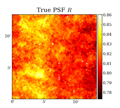
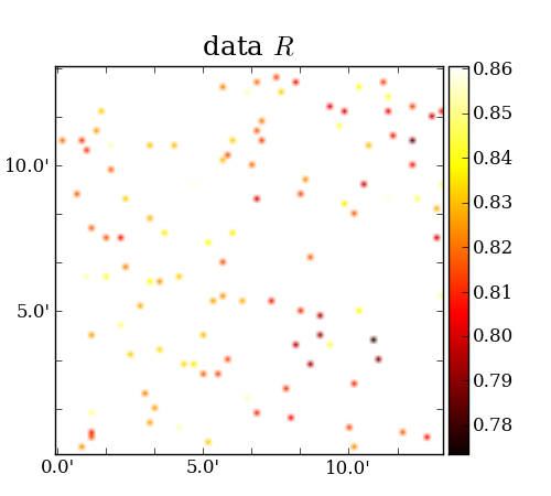
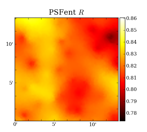
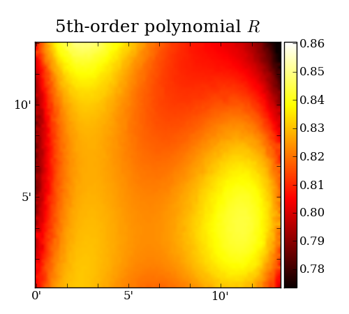
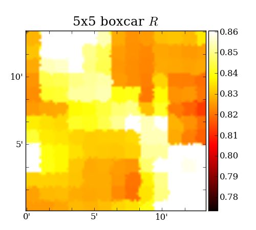
Figure 11: Illustration for interpolation of PSF size (FWHM size in arcseconds). The top map shows the “true” PSF size field that we would like to reconstruct from the stellar data in the second map, the observed stellar size. The next three maps show model maps constructed with psfent, a 5th-order polynomial fit and a 5$\times$ 5-pixel boxcar smoothing, respectively. The atmospheric PSF pattern and stellar density is the same as that in Figure 5 (b).

Appendix C Correlation between ellipticity components

We have argued in Section 3.1 that the two ellipticity components should be independent from each other in each exposure, while both varying with similar amplitudes and spatial structures between different exposures. In this appendix we demonstrate this by calculating the following three spatial correlation functions for the 100 “true” PSF images:

$$\xi_{11}(\theta)=\langle\varepsilon_{1}(\theta_{0})\varepsilon_{1}(\theta_{0}+\theta)\rangle;$$ (15)

$$\xi_{22}(\theta)=\langle\varepsilon_{2}(\theta_{0})\varepsilon_{2}(\theta_{0}+\theta)\rangle;$$ (16)

$$\xi_{12}(\theta)=\langle\varepsilon_{1}(\theta_{0})\varepsilon_{2}(\theta_{0}+\theta)\rangle.$$ (17)

In Figure 12, the three correlation functions are shown, each representing the median of the 100 realisations in the sample, with the error bars showing the standard deviation of the 100 realisations divided by $\sqrt{100}$. The $\xi_{11}$ and $\xi_{22}$ curves are clearly positive and show similar structures. The difference in the two curves may be due to sample variance, and the fact that there are no rotation/dithering between these exposures. On the other hand, $\xi_{12}$ is consistent with zero. This supporting our argument that the “phase” of the two ellipticity components are independent of each other, while the spatial power spectrum is similar.

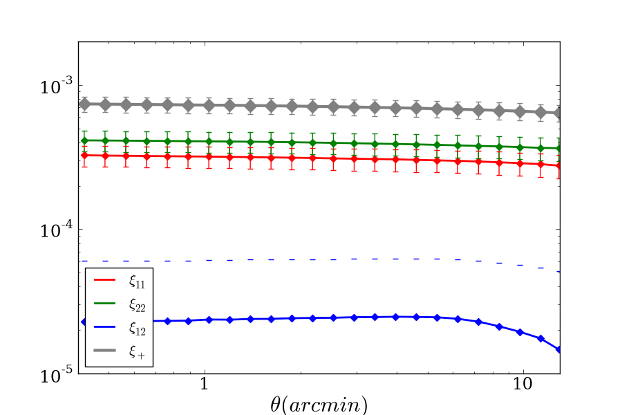
Figure 12: Three diagnostic correlation functions $\xi_{11}$ (red), $\xi_{22}$ (green) and $\xi_{12}$ (blue), plotted with the full ellipticity correlation function $\xi_{+}$ (grey). Each curve represents the median of the 100 different atmosphere realisations. The error bars indicate the rms spread in the 100 exposures divided by $\sqrt{100}$.

References

- Albrecht et al. (2006) Albrecht A., et al., 2006, ArXiv Astrophysics e-prints
- Amara & Réfrégier (2008) Amara A., Réfrégier A., 2008, MNRAS, 391, 228
- Bartelmann & Schneider (2001) Bartelmann M., Schneider P., 2001, Physics Reports, 340, 291
- Benjamin et al. (2007) Benjamin J., et al., 2007, MNRAS, 381, 702
- Bergé et al. (2012) Bergé J., Price S., Amara A., Rhodes J., 2012, MNRAS, 419, 2356
- Bertin & Arnouts (1996) Bertin E., Arnouts S., 1996, A&AS, 117, 393
- Bridle et al. (2010) Bridle S., et al., 2010, MNRAS, 405, 2044
- Chang et al. (2012) Chang C., et al., 2012, in preparation
- Connolly et al. (2010) Connolly A. J., et al., 2010, in SPIE Conference Series Vol. 7738, Simulating the LSST system
- de Vries et al. (2007) de Vries W. H., et al., 2007, ApJ, 662, 744
- Gull & Skilling (1999) Gull S., Skilling J., 1999, Quantified Maximum Entropy MemSys5 Users’ Manual. Maximum Entropy Data Consultants Ltd., Version 1.2 edn
- Hetterscheidt et al. (2006) Hetterscheidt M., et al., 2006, The Messenger, 126, 19
- Hetterscheidt et al. (2007) Hetterscheidt M., et al., 2007, A&A, 468, 859
- Heymans et al. (2006) Heymans C., et al., 2006, MNRAS, 368, 1323
- Heymans et al. (2012) Heymans C., et al., 2012, MNRAS, 421, 381
- Hoekstra (2004) Hoekstra H., 2004, MNRAS, 347, 1337
- Hoekstra et al. (2006) Hoekstra H., et al., 2006, ApJ, 647, 116
- Hu & Tegmark (1999) Hu W., Tegmark M., 1999, ApJ, 514, L65
- Ivezic et al. (2008) Ivezic Z., et al., 2008, ArXiv e-prints: astro-ph/0805.2366
- Jain et al. (2006) Jain B., Jarvis M., Bernstein G., 2006, Journal of Cosmology and Astroparticle Physics, 2, 1
- Jain & Seljak (1997) Jain B., Seljak U., 1997, ApJ, 484, 560
- Jarvis et al. (2006) Jarvis M., et al., 2006, ApJ, 644, 71
- Jarvis & Jain (2004) Jarvis M., Jain B., 2004, ArXiv e-prints: astro-ph/0412234
- Jurić et al. (2008) Jurić M., et al., 2008, ApJ, 673, 864
- Kaiser et al. (1995) Kaiser N., Squires G., Broadhurst T., 1995, ApJ, 449, 460
- Kitching et al. (2012a) Kitching T. D., et al., 2012a, MNRAS, 423, 3163
- Kitching et al. (2012b) Kitching T. D., et al., 2012b, ArXiv e-prints: astro-ph/1204.4096
- Kolmogorov (1992) Kolmogorov A., 1992, Dokl. Akad. Nauk SSSR, 30, 301
- Lane, R. G. (1992) Lane, R. G. Glindemann, A. D., 1992, Waves in Random Media, 2, 209
- Maisinger et al. (2004) Maisinger K., Hobson M. P., Lasenby A. N., 2004, MNRAS, 347, 339
- Massey et al. (2002) Massey R., et al., 2002, in N. Metcalfe & T. Shanks ed., A New Era in Cosmology Vol. 283 of Astronomical Society of the Pacific Conference Series, Cosmic Shear with Keck: Systematic Effects. pp 193–+
- Massey et al. (2007) Massey R., Heymans C., Bergé 2007, MNRAS, 376, 13
- Miller et al. (2007) Miller L., et al., 2007, MNRAS, 382, 315
- Paulin-Henriksson et al. (2008) Paulin-Henriksson S., et al., 2008, A&A, 484, 67
- Peterson et al. (2009) Peterson J. R., et al., 2009, LSST Science Book, Version 2.0, Chapter 3.3
- Peterson et al. (2012) Peterson J. R., et al., 2012, in preparation
- Rhodes et al. (2007) Rhodes J. D., et al., 2007, ApJS, 172, 203
- Schneider (1992) Schneider P., 1992, in Kayser R., Schramm T., Nieser L., eds, Gravitational Lenses Vol. 406 of Lecture Notes in Physics, Berlin Springer Verlag, Gravitational Lensing Statistics. p. 196
- Schneider et al. (2002) Schneider P., et al., 2002, A&A, 396, 1
- Schrabback et al. (2010) Schrabback T., et al., 2010, A&A, 516, A63+
- Semboloni et al. (2006) Semboloni E., et al., 2006, A&A, 452, 51
- Van Waerbeke et al. (2002) Van Waerbeke L., et al., 2002, A&A, 393, 369
- Van Waerbeke et al. (2005) Van Waerbeke L., Mellier Y., Hoekstra H., 2005, A&A, 429, 75
- Weir (1992) Weir N., 1992, in D. M. Worrall, C. Biemesderfer, & J. Barnes ed., Astronomical Data Analysis Software and Systems I Vol. 25 of Astronomical Society of the Pacific Conference Series, A Multi-Channel Method of Maximum Entropy Image Restoration. pp 186–+
- Wittman (2005) Wittman D., 2005, ApJ, 632, L5