Searching for Realizations of Finite Metric Spaces in Tight Spans
Abstract
An important problem that commonly arises in areas such as internet traffic-flow analysis, phylogenetics and electrical circuit design, is to find a representation of any given metric on a finite set by an edge-weighted graph, such that the total edge length of the graph is minimum over all such graphs. Such a graph is called an optimal realization and finding such realizations is known to be NP-hard. Recently Varone presented a heuristic greedy algorithm for computing optimal realizations. Here we present an alternative heuristic that exploits the relationship between realizations of the metric and its so-called tight span . The tight span is a canonical polytopal complex that can be associated to , and our approach explores parts of for realizations in a way that is similar to the classical simplex algorithm. We also provide computational results illustrating the performance of our approach for different types of metrics, including -distances and two-decomposable metrics for which it is provably possible to find optimal realizations in their tight spans.
keywords:
combinatorial optimization , metric , graph , realization , tight span1 Introduction
An important problem that commonly arises in areas such as internet traffic-flow analysis [9], phylogenetics [2] and electrical circuit design [18], is to realize any given metric on some finite set by an edge-weighted graph with labeling its vertex set, often with the additional requirement that the total edge length of the graph is minimum. This can be useful, for example, for visualizing the metric, or for trying to better understand its structural properties. More formally this optimization problem can be stated as follows. A realization of is a connected graph with vertex set and edge set , together with an edge-weighting and a labeling map such that, for all , equals , that is, the length of a shortest path from to in (cf. Figure 1(a) and (b)). The problem then is to find an optimal realization of , that is, a realization of that has minimum total edge length over all possible realizations of .
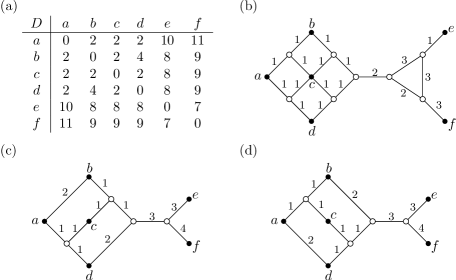
Early work on optimal realizations started with [18] (see also [29] for a comprehensive list of references), which focused mainly on special classes of metrics such as, for example, those that admit an optimal realization where the underlying graph is a tree (so-called treelike metrics). Subsequently it was found that every metric on a finite set has an optimal realization [23], although this need not be unique (cf. Figure 1(c) and (d)). There even always exists an optimal realization of with vertices [12, p. 392], which implies that there is an exhaustive algorithm to search for an optimal realization. However, it was also shown that computing an optimal realization is NP-hard [1, 30]. More recently, there has been renewed interest in computational aspects of this problem. For example, in [21, 22] (see also [13]) a way to break up the problem of computing an optimal realization into subproblems using so-called cut points is presented, and in [29] a heuristic is presented for computing optimal realizations.
Here we present an alternative heuristic for systematically computing optimal realizations that exploits the relationship between optimal realizations of a metric and its so-called tight span [12, 24]. In brief (see Section 2 for details), is a polytopal complex (essentially a union of polytopes) that can be canonically associated to which is itself a (non-finite) metric space and into which the metric can be canonically embedded. Remarkably, in [12] it is shown that the 1-skeleton of (i.e., the edge-weighted graph formed essentially by taking all of the 0- and 1-dimensional faces of ) is always a realization of . Moreover, Dress conjectured [12, (3.20)] that some optimal realization of can always be obtained by removing some set of edges from .
While Dress’ conjecture is still open for metrics in general, recently it has been shown to hold for the class of so-called two-decomposable metrics [20, Theorem 1.2], a class which includes treelike metrics and -distances between points in the plane (see Section 3 for more details). In particular, this and the aforementioned result in [12] suggest that it could be useful to consider as a “search space” in which to look for some optimal realization of (or at least some interesting realization of which has relatively small total edge length).
Guided by this principle, given an arbitrary finite metric , in Section 4 we propose a heuristic for computing a realization of that is a subgraph of . This heuristic explores parts of in a way similar to the classical simplex algorithm [11]. Moreover, it does not explicitly compute , whose vertex set can have cardinality that is exponential in (see e.g. [19] for some explicit bounds). We also show that the heuristic is guaranteed to find optimal realizations for some simple types of metrics.
Since, as mentioned above, the problem of finding optimal realizations is NP-hard, we assess the performance of our new heuristic using two strategies. First, we consider a special instance of the problem where we take metrics to be -distances between points in the plane. In Section 5 we show that finding optimal realizations of such a metric in is equivalent to the so-called minimum Manhattan network problem (which was also recently shown to be NP-hard [7]). This allows us to compare the realizations computed by our heuristic with realizations computed using a mixed integer linear program (MIP) for the minimum Manhattan network problem presented in [3] (see also [26] for a comprehensive list of references on other approaches for solving this well-studied problem). Second, in Section 6 we describe a mixed integer program (MIP) for computing a minimal subrealization of a realization of some metric, that is, a subrealization with minimum total edge length. This allows us to obtain some impression of how close the realizations computed by our heuristic are to a minimal subrealization of in case is not too large. Moreover, in case the metric is two-decomposable, a minimal subrealization of is (by the aforementioned result in [20]) an optimal realization and so we can compare the realizations computed by our new heuristic with optimal ones for this special class of metrics.
Based on these considerations, in Section 7 we present simulations for -distances, two-decomposable metrics and random metrics to assess the performance of our heuristic. An implementation of this heuristic is freely available for download at www.uea.ac.uk/cmp/research/cmpbio/CoMRiT/. This includes the algorithm for efficiently computing cut points as described in [13] and auxiliary programs that allow to generate the MIP description for the minimum Manhattan network problem, as well as for the problem of computing a minimal subrealization so that they can be solved using existing MIP solvers (we used the solver that is part of the GNU linear programming kit (www.gnu.org/software/glpk/) in our experiments). We conclude the paper with a brief discussion of some possible future directions in Section 8.
2 Preliminaries
In this section, we first recall the formal definition of the tight span of a metric, a concept that has been discovered and re-discovered several times in the literature (see e.g. [8, 12, 24]). We also recall some facts concerning tight spans and optimal realizations that will be used later on (for more on this see e.g. [14, Chapter 5]).
2.1 Some tight span theory
A finite metric space is a pair consisting of a finite non-empty set and a symmetric bivariate map such that and for all . To emphasize that does not necessarily imply , such a map is often called a pseudometric, but we will simply refer to as a metric here. A map from a metric space into a metric space is an isometric embedding if for all .
Now, given any finite metric space , the tight span is defined to be the polytopal complex (see e.g. [25]) that is the union of the bounded faces of the polyhedron
Viewed as a subset of , can be endowed with the -metric which is defined by
for all so that is also a (non-finite!) metric space. Note that there exists a canonical isometric embedding of into , the so-called Kuratowski embedding [27], that maps every to . Note that the map is a 0-dimensional face (or vertex) of for every and, therefore, it is contained in the 1-skeleton .
Later we will use the fact that the tight span can be viewed as a hull of the given metric space similar to the convex hull associated to a set of points in Euclidean space. To make this more precise, define a map from a metric space into a metric space to be non-expansive if for all , and a metric space to be injective if for every metric space and every subset any non-expansive map of the subspace into can be extended to a non-expansive map of into . The tight span satisfies the following universal property [12, 24]:
Lemma 1.
Any isometric embedding of a metric space into an injective metric space can be extended to an isometric embedding of into .
2.2 Tight spans and optimal realizations
We now present a key relationship between realizations and tight spans that was first discovered by Dress. Let be an arbitrary finite metric space and the graph that forms the 1-skeleton of . Defining the map by putting for all edges of and the map by putting for all , it is shown in [12, Theorem 5] that is a realization of (see also [14, Theorem 5.15]). Moreover, in [12] it is shown that, for any optimal realization of , there exists a map with for all that preserves certain distances, that is, for all edges . While this suggests that every optimal realization of is somehow ’contained’ in , in [1] it was shown that there exists an infinite family of optimal realizations of a certain metric on six points, for which no member is isomorphic to some subrealization of the 1-skeleton of . Still, as mentioned in the introduction, it is not known whether or not there always exists some optimal realization of that is a subrealization of .
3 Two-decomposable metrics
Before we present our heuristic in the next section, we shall briefly consider a special class of finite metrics , the two-decomposable metrics, for which it is known that always contains a subrealization that is an optimal realization of . As mentioned in the introduction, these metrics are of interest as we can in principle compute optimal realizations for them exactly and thus measure the accuracy of our heuristic for computing realizations for small metric spaces.
We first need to recall some relevant concepts. A split of a finite set is a bipartition of into two non-empty subsets and , also denoted by . For any , that set in that contains is denoted by and the other set by . Two splits and of are compatible if at least one of the intersections , , and is empty. Otherwise the two splits are incompatible. A set of splits of is called a split system (on ). A split system is two-compatible if there is no subset with and any two distinct splits in are incompatible.
Now, for any split of , define the metric on putting, for all , if and otherwise. A metric on is two-decomposable if there exists a two-compatible split system on and a weighting with . We also say that is induced by and the weighting . Later we will use the following result [20, Theorem 1.2]:
Theorem 2.
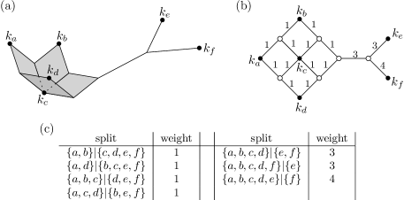
Let be a two-decomposable metric on . Then there always exists an optimal realization that is a subrealization of . In particular, there exists an optimal realization of such that there exists an injective map with for all edges and for all .
We illustrate this theorem in Figure 2. More specifically, the metric in Figure 1(a) is two-decomposable, and its tight span is depicted in Figure 2(a). The realization is pictured in Figure 2(b), and a two-compatible split system associated to is given in Figure 2(c). Note that both of the optimal realizations for given in Figure 1(c) and (d) can be obtained from by removing precisely two edges.
We now prove two simple but useful facts concerning the relationship between -distances between points in the plane, two-decomposable metrics and treelike metrics. For a point we denote by and the - and -coordinate of , respectively, and the -distance between two points by . Then we have:
Lemma 3.
Let be a finite non-empty set of points in . Then the metric is
-
(i)
two-decomposable.
-
(ii)
the sum of two treelike metrics.
Proof.
(i) Let be the set of those splits of for which there exists a real number such that and . Similarly, let be the set of those splits of for which there exits a real number such that and . For every , put and, for every put . Note that any two splits in as well as any two splits in are compatible. Hence, the split system is two-compatible.
Now, define, for any split in , the weight
It is not hard to check that , implying that is indeed two-decomposable.
(ii) Continuing to use the notation introduced in the proof of (i), note that we have with and . Therefore, it remains to note that and are treelike in view of the fact that a metric space is treelike if there exists a system of pairwise compatible splits of and a map with [4]. ∎
4 Computing a realization in the tight span
We now present our algorithm for computing realizations using the tight span. We also prove that it is guaranteed to yield an optimal solution for some special types of metrics. Given a finite metric space , the basic idea of our algorithm is to select, for each pair of distinct elements in , a shortest path from to in . The union of these paths is then a realization of . This is summarized in the form of pseudo-code in Algorithm 1.
Pseudocode for the function find_path is presented in Algorithm 2. This function essentially computes, for any vertex of and any , a shortest path from to in . To avoid computing the whole graph , it constructs such a path edge by edge employing the polyhedron as follows. It computes in polynomial time from the description of all vertices of that are adjacent to in . Among these vertices, one with that minimizes is selected. We refer to this as a simplex step from that arrives at vertex , since this is similar to one step in Dantzig’s well-known simplex algorithm [11].
To make use of the fact that certain edges of might have been added to in previous rounds of the foreach-loop in Algorithm 1, the function find_path first explores whether the current graph already contains edges that can serve as the initial part of a suitable path from to . One would expect that the choice of the order in which pairs are processed in the foreach-loop has some impact on how many edges can be re-used in subsequent rounds. We found that ordering the pairs according to increasing distances between them tends to work well in practice. Then, in particular, for any elements with , no edges will be added when processing the pair .
Note that our algorithm is guaranteed to output an optimal realization for any treelike metric and any metric that corresponds to the shortest path distances between the pairs of vertices of a graph that is a cycle. The former follows from the fact that, for any treelike metric, is a tree [12], and the latter is an immediate consequence of the fact that we process the pairs of elements in according to increasing distances between them. Moreover, using the decomposition of a given metric according to [21, 22] as a preprocessing step, it follows that an optimal realization can be obtained for a given metric if the decomposition of yields only subinstances for which our algorithm outputs an optimal realization. In particular, it follows that our algorithm produces optimal realizations for all inputs given in the appendix of [29].
5 Minimum Manhattan networks and optimal realizations
In this section, using properties of the tight span, we give a concise proof of the fact that the problem of computing a minimum Manhattan network is nothing other than the problem of computing an optimal realization for a special class of finite metric spaces (see also [15] for related work). This allows us to directly compare our heuristic for computing realizations with some existing algorithms for computing minimum Manhattan networks. Note that this fact seems to have not been pointed out before in the literature and has some interesting consequences for the computational complexity of constructing an optimal realization which we shall also point out.
To state the main result of this section, we first introduce some more notation. A Manhattan network consists of a finite graph whose vertex set is a set of points in the plane and a map that assigns to each edge as its length the -distance between the points and . In addition, we require that, for every edge , the straight line segment with endpoints and is either horizontal or vertical and, for any two distinct edges and in , the straight line segments and do not cross, that is, . For any path from to in , denotes the length of , and is monotone if .
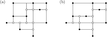
Now, given a finite set of points , a Manhattan network for is a Manhattan network with such that for any two distinct there exists a monotone path from to in . Such a network is called minimum if its total length is minimum among all Manhattan networks for (cf. Figure 3). The minimum Manhattan network problem has been studied by several researchers over the last few years (for a comprehensive list of references for this problem see e.g. [26]). We have the following relationship between minimum Manhattan networks and optimal realizations:
Theorem 4.
Let be a finite non-empty set of points in . Then, for any minimum Manhattan network for , is an optimal realization of , where is the identity map on .
Proof.
By definition, any Manhattan network for is, up to adding the map , a realization of . Hence, it suffices to show that there exists a Manhattan network for whose total length is at most the total length of some optimal realization of .
Consider an optimal realization of such that there exists an injective map with for all edges and for all . By Lemma 3 and Theorem 2, such an optimal realization always exists.
Now, since the metric space is injective (see e.g. [5]), it follows that for every finite set of points in there exists an isometric embedding of into that maps every , , to . Therefore, there exists an injective map with for all edges and for all . To obtain a Manhattan network for , start with the points in and then add, step by step, for every , edges to obtain a monotone path from to (if an edge on this monotone path crosses an edge added in some previous step, we place an additional vertex at the point where and cross to remove the crossing). Note that in the resulting Manhattan network the length of a shortest path between and can be at most the length of a shortest path between and in for all . This implies that there is a monotone path from to in for all . Hence, is indeed a Manhattan network for . Finally, the total length of is, by construction, not larger than the total length of , as required. ∎
Before concluding this section, we point out some interesting implications of the last result:
Corollary 5.
Computing an optimal realization of a finite metric space is NP-hard even if
-
(i)
is two-decomposable, or
-
(ii)
is the sum of two treelike metrics on .
Proof.
In [7] it is shown that computing (even just the total edge length of) a minimum Manhattan network is NP-hard. In view of Theorem 4, this implies that computing an optimal realization of for a given point set is NP-hard. By Lemma 3(i) the metric is two-decomposable. This establishes (i). Alternatively, this also follows from the NP-hardness proof in [1]: It can be checked that the metric that arises from applying the reduction is always two-decomposable.
In Lemma 3(ii) it was shown that is even the sum of two treelike metrics on . This establishes (ii). ∎
6 Finding minimal subrealizations
In a similar spirit to finding optimal realizations, there is a whole family of so-called inverse shortest path problems (see e.g. [10] and the references therein). In these problems, one has a collection of allowed edit operations on graphs such as, for example, deleting edges or, if a graph has weights assigned to its edges, changing these weights. Each edit operation has an associated cost. Then, given a graph and required distances between certain pairs of vertices in , a minimum cost editing of is sought so that in the resulting graph the shortest path distances between the specified pairs equal the given distances. The problem of finding a minimal subrealization mentioned in the introduction can be viewed as yet another variant of this theme and we will briefly collect some facts about it in this section.
First note that, in view of the fact that the problem of computing a minimum Manhattan network is NP-hard [7] and the fact that there is always a minimum Manhattan network that is contained in the grid induced by the given point set (see e.g. [3]), we have:
Proposition 6.
The problem of computing a minimal subrealization of a given realization is NP-hard even if is a two-dimensional grid graph.
Next note that, following a similar approach to the one used in [3] for computing a minimum Manhattan network, one can phrase the problem of computing a minimal subrealization as a MIP. For the convenience of the reader, we include below the description of the MIP that we used for benchmarking in the computational experiments and that yields, for any given realization of a finite metric space , a subgraph of with minimum total edge length such that is also a realization of :
-
1.
For every edge , we introduce two directed edges from to and from to . Let denote the set of these directed edges.
-
2.
For every edge , we have a binary variable indicating whether or not is an edge of .
-
3.
For any two distinct elements , we send one unit of flow from to that ensures that there is at least one path from to of length in . To describe this flow, we introduce, for every directed edge , a real-valued variable .
-
4.
For any two distinct elements , the variables must satisfy the following constraints:
-
(1)
and for all .
-
(2)
for all .
-
(3)
for .
-
(4)
for .
-
(5)
.
-
(1)
-
5.
The objective function is
In practice, we found that the size of the MIP can often be reduced considerably by only introducing the variable for those edges that actually lie on some shortest path from to in .
7 Computational Experiments
To perform computational experiments, we have implemented the algorithm described in Section 4 in C++ as an extension to the mathematical software system polymake [16]. In this implementation, we apply, as a preprocessing step, the decomposition of a given metric according to [21, 22].
The experiments are designed to give an impression of the range of inputs that can be attacked by our algorithm in terms of size and also how close the realization produced by our algorithm is to an optimal realization. For each size of the ground set of the metric space, 100 randomly generated inputs were considered and we present the mean run time of our algorithm (including the preprocessing) and the mean ratio between the length of the realization produced by our algorithm and a minimal subrealization of (if available). The variance of these values was usually quite low and is omitted.
| 5 | 0.28 | 0.24 | 1.01 | 0.01 | 0.40 | 0.93 |
| 10 | 0.65 | 0.41 | 1.15 | 0.07 | 2.23 | 0.66 |
| 15 | 1.46 | 0.70 | 1.22 | 4.11 | 18.90 | 0.55 |
| 20 | 3.07 | 1.12 | 1.27 | 254.49 | 386.28 | 0.50 |
| 25 | 7.78 | 1.47 | 1.30 | 15075.02 | 7690.96 | 0.46 |
| 30 | 11.49 | 2.04 | 1.34 | |||
| 35 | 21.25 | 2.84 | 1.37 | |||
| 40 | 37.99 | 4.03 | 1.39 | |||
| 45 | 64.61 | 5.68 | 1.41 | |||
| 50 | 105.42 | 7.89 | 1.42 | |||
| 55 | 167.75 | 11.27 | 1.43 | |||
| 60 | 256.51 | 16.66 | 1.44 | |||
| 65 | 379.84 | 22.79 | 1.45 | |||
| 70 | 555.02 | 31.90 | 1.47 | |||
| 75 | 791.90 | 43.60 | 1.48 | |||
| 80 | 1110.62 | 61.06 | 1.49 | |||
| 85 | 1838.51 | 116.24 | 1.50 | |||
| 90 | 2229.85 | 124.47 | 1.50 |
In the tables, denotes the time to compute the whole tight span (if the size if the tight span admitted to compute it using polymake), denotes the time needed to solve the MIP described in Section 6 using the solver glpksol from the GNU linear programming kit, and denotes the ratio of the length of the realization produced by our algorithm to the total edge length of the whole 1-skeleton of the tight span. A indicates that the corresponding value could not be obtained because the 1-skeleton of the tight span was too large or at least too large to solve the resulting MIP. All run times were taken on a Intel(R) Core(TM)2 Quad CPU 2.66GHz machine running CentOs 5.6 using only one core.
7.1 Manhattan networks
Inputs were generated by choosing random points on an integer grid. In addition to the MIP described in Section 6, we also used the MIP presented in [3] to compute an optimal realization for each input point set. The run time for solving this alternative MIP using glpksol is also given in Table 1. As can be seen, the realizations we obtain are usually within a factor of the optimum that is slowly growing with reaching for the largest instances considered in our experiments. Note that there exist several polynomial time algorithms that guarantee to produce a realization whose length is within a constant factor of the optimum — currently, for the best known algorithms, the factor is 2 [6, 17, 28].
7.2 Two-decomposable metrics
Recall that, in case the metric is two-decomposable, we know that there exists an optimal realization that is a subrealization of (see Section 3). Hence, is actually the ratio between the length of the realization produced by our algorithm and the length of an optimal realization. We tested two types of two-decomposable metrics (cf. Table 2):
| 5 | 0.46 | 0.01 | 0.43 | 1.02 | 0.95 |
|---|---|---|---|---|---|
| 10 | 1.46 | 0.07 | 2.05 | 1.10 | 0.77 |
| 15 | 3.00 | 3.49 | 6.83 | 1.16 | 0.70 |
| 20 | 5.44 | 225.32 | 43.73 | 1.19 | 0.66 |
| 25 | 9.18 | 13174.89 | 314.37 | 1.22 | 0.63 |
| 30 | 12.87 | ||||
| 35 | 24.13 | ||||
| 40 | 38.62 | ||||
| 45 | 75.90 | ||||
| 50 | 114.40 | ||||
| 55 | 169.91 | ||||
| 60 | 250.89 | ||||
| 65 | 363.25 | ||||
| 70 | 506.94 | ||||
| 75 | 587.90 | ||||
| 80 | 844.98 | ||||
| 85 | 1090.04 | ||||
| 90 | 1319.21 | ||||
| 100 | 2143.58 |
| 5 | 0.45 | 0.01 | 0.49 | 1.04 | 0.81 |
|---|---|---|---|---|---|
| 10 | 1.06 | 0.07 | 2.00 | 1.16 | 0.67 |
| 15 | 2.29 | 3.49 | 9.42 | 1.17 | 0.59 |
| 20 | 21.05 | 222.07 | 83.64 | 1.22 | 0.58 |
Metrics that are the sum of two treelike metrics: We choose two random binary trees with leaves, took the set of these leaves as the ground set of the metric space and assigned uniformly distributed lengths (between 1 and ) to the edges of the trees. Then we formed the sum of the two treelike metrics realized by the binary trees.
Metrics resulting from random two-compatible split systems: We generated random two-compatible split systems of size by generating random splits and adding them to an initially empty system if it remains two-compatible after adding the split. The metric considered in the experiment is the metric induced by the resulting split system where we again assigned uniformly distributed weights to the splits.
7.3 Random metrics
Finally, we generated random metrics on a ground set with elements by choosing each pairwise distance uniformly between and . The results are presented in Table 3. Note that in this experiment it is not known whether contains an optimal realization of the given metric as a subrealization. Therefore, the value is only a lower bound on the ratio between the length of the realization produced by our algorithm and the length of an optimal realization.
| 5 | 0.48 | 0.01 | 0.53 | 1.04 | 0.90 |
|---|---|---|---|---|---|
| 6 | 0.72 | 0.01 | 1.80 | 1.06 | 0.74 |
| 7 | 0.88 | 0.02 | 3.46 | 1.10 | 0.56 |
| 8 | 1.35 | 0.04 | 10.12 | 1.15 | 0.39 |
| 9 | 1.31 | 0.12 | 758.07 | 1.20 | 0.26 |
| 10 | 1.32 | 0.35 | 33652.08 | 1.21 | 0.18 |
| 15 | 3.52 | 300.29 | 0.01 | ||
| 25 | 15.97 | ||||
| 30 | 40.47 | ||||
| 35 | 84.81 | ||||
| 40 | 181.73 | ||||
| 45 | 330.98 | ||||
| 50 | 545.36 | ||||
| 55 | 749.25 | ||||
| 60 | 1204.18 | ||||
| 65 | 2081.53 |
8 Discussion
Our computational experiments suggest that it might be interesting to investigate whether our heuristic (or a suitable variant of it) yields a constant-factor approximation algorithm for computing an optimal realization, at least for certain classes of metrics such as, for example, two-decomposable metrics.
We also see that our algorithm can produce realizations for metric spaces with up to 50 elements, even in the case of general random metrics. Note also that all computations are done with arbitrary precision rationals/integers, to ensure combinatorial accuracy. Using floating point numbers instead (which would make sense at least for the general random metrics, that is, generic metrics) could further speed up the computations.
In future work, it could also be interesting to try and develop an exact, exponential time algorithm for computing an optimal realization. This would be helpful for benchmarking heuristics but would also allow to check Dress’ conjecture for more examples. We expect that this could at least give some interesting further insights into the structure of the problem.
Acknowledgments
We would like to thank the two reviewers for their helpful comments.
References
- [1] I. Althöfer. On optimal realizations of finite metric spaces by graphs. Discrete and Computational Geometry, 3:103–122, 1988.
- [2] H.-J. Bandelt and A. Dress. Split decomposition: a new and useful approach to phylogenetic analysis of distance data. Molecular Phylogenetics and Evolution, 1:242–252, 1992.
- [3] M. Benkert, A. Wolff, F. Widmann, and T. Shirabe. The minimum Manhattan network problem: approximations and exact solutions. Computational Geometry, 35:188–208, 2006.
- [4] P. Buneman. The recovery of trees from measures of dissimilarity. In F. Hodson et al., editor, Mathematics in the Archaeological and Historical Sciences, pages 387–395. Edinburgh University Press, 1971.
- [5] N. Catusse, V. Chepoi, and Y. Vaxès. Embedding into the rectilinear plane in optimal time. Theoretical Computer Science, 412:2425–2433, 2011.
- [6] V. Chepoi, K. Nouioua, and Y. Vaxès. A rounding algorithm for approximating minimum Manhattan networks. Theoretical Computer Science, 390:56–69, 2008.
- [7] F. Chin, Z. Guo, and H. Sun. Minimum Manhattan network is NP-complete. In Proc. Annual Symposium on Computational Geometry, pages 393–402. ACM press, 2009.
- [8] M. Chrobak and L. Larmore. Generosity helps or an 11-competitive algorithm for three servers. Journal of Algorithms, 16:234–263, 1994.
- [9] F. Chung, M. Garrett, R. Graham, and D. Shallcross. Distance realization problems with applications to internet tomography. Journal of Computer and System Sciences, 63:432–448, 2001.
- [10] T. Cui and D. Hochbaum. Complexity of some inverse shortest path lengths problems. Networks, 56:20–29, 2010.
- [11] G. Dantzig. Linear programming and extensions. Princeton University Press, Princeton, N.J., 1963.
- [12] A. Dress. Trees, tight extensions of metric spaces, and the cohomological dimension of certain groups: a note on combinatorial properties of metric spaces. Advances in Mathematics, 53:321–402, 1984.
- [13] A. Dress, K. Huber, J. Koolen, V. Moulton, and A. Spillner. An algorithm for computing cutpoints in finite metric spaces. Journal of Classification, 27:158–172, 2010.
- [14] A. Dress, K. Huber, J. Koolen, V. Moulton, and A. Spillner. Basic phylogenetic combinatorics. Cambridge University Press, 2012.
- [15] D. Eppstein. Optimally fast incremental Manhattan plane embedding and planar tight span construction. Journal of Computational Geometry, 2:144–182, 2011.
- [16] E. Gawrilow and M. Joswig. polymake: a framework for analyzing convex polytopes. In Polytopes–combinatorics and computation (Oberwolfach, 1997), volume 29 of DMV Sem., pages 43–73. Birkhäuser, Basel, 2000.
- [17] Z. Guo, H. Sun, and H. Zhu. A fast 2-approximation algorithm for the minimum Manhattan network problem. In Proc. International Conference Algorithmic Aspects in Information and Management, volume 5034 of LNCS, pages 212–223. Springer, 2008.
- [18] S. Hakimi and S. Yau. Distance matrix of a graph and its realizability. Quarterly of Applied Mathematics, 22:305–317, 1964.
- [19] S. Herrmann and M. Joswig. Bounds on the -vectors of tight spans. Contributions to Discrete Mathematics, 2:161–184, 2007.
- [20] S. Herrmann, J. Koolen, A. Lesser, V. Moulton, and T. Wu. Optimal realisations of two-dimensional, totally-decomposable metrics, 2011. preprint arXiv:1108.0290.
- [21] A. Hertz and S. Varone. The metric bridge partition problem: partitioning of a metric space into two subspaces linked by an edge in any optimal realization. Journal of Classification, 24:235–249, 2007.
- [22] A. Hertz and S. Varone. The metric cutpoint partition problem. Journal of Classification, 25:159–175, 2008.
- [23] W. Imrich, J. Simões-Pereira, and C. Zamfirescu. On optimal embeddings of metrics in graphs. Journal of Combinatorial Theory, Series B, 36:1–15, 1984.
- [24] J. Isbell. Six theorems about metric spaces. Commentarii Mathematici Helvetici, 39:65–74, 1964.
- [25] V. Klee and P. Kleinschmidt. Convex polytopes and related complexes. In R. Graham, M. Grötschel, and L. Lovász, editors, Handbook of Combinatorics, Part I, pages 875–917. Elsevier, 1999.
- [26] C. Knauer and A. Spillner. A fixed-parameter algorithm for the minimum manhattan network problem. Journal of Computational Geometry, 2:189–204, 2011.
- [27] C. Kuratowski. Quelques problèmes concernant les espaces métriques non-separables. Fundamenta Mathematica, 25:534–545, 1935.
- [28] K. Nouioua. Enveloppes de Pareto et réseaux de Manhattan. PhD thesis, L’Université de la Méditerranée, 2005.
- [29] S. Varone. A constructive algorithm for realizing a distance matrix. European Journal of Operational Research, 174:102–111, 2006.
- [30] P. Winkler. Isometric embeddings in products of complete graphs. Discrete Applied Mathematics, 7:221–225, 1984.