$p_{\perp}$-broadening and production processes versus dipole/quadrupole amplitudes at next-to-leading order

Abstract

Through the systematic inspection of graphs in the framework of lightcone perturbation theory, we demonstrate that an identity between the evolution of $p_{\perp}$-broadening amplitudes with the energy and the evolution of forward scattering amplitudes of color dipoles off nuclei holds at next-to-leading order accuracy. In the general case, the relation is not a graph-by-graph correspondence, neither does it hold strictly speaking for definite values of the momenta: Instead, it relates classes of graphs of similar topologies, and in some cases, the matching requires an analytical continuation in the appropriate longitudinal momentum variable. We check that the same kind of relation is also true at next-to-leading order between amplitudes for the production of dijets and quadrupole forward amplitudes.

1 Introduction

Observables such as dijet correlations [1, 2] or other production processes in proton-nucleus scattering are outstanding probes of the high-density regime of QCD, and are likely to become one of the major focusses of the QCD community in the next few years.

Preliminary phenomenological works [3] have shown that saturation models have the ability to describe successfully the present data. In order to confirm these results and provide accurate predictions for the Large Hadron Collider, firm theoretical foundations for the calculation of these production processes are now needed.

One outstanding problem in this program is the energy (or equivalently, the Bjorken-$x$) dependence of the considered observables. The formalism to compute the energy evolution of forward amplitudes has reached a certain degree of sophistication: The evolution is known to be given by the Balitsky-Fadin-Kuraev-Lipatov (BFKL) equation [4, 5, 6], whose kernel is established at next-to-leading order in $\ln 1/x$ [7, 8] see e.g. [9, 10] for references and for the state of the art of the phenomenology of deep-inelastic scattering. But production processes have not received the same attention so far.

Interesting relations between production processes and forward amplitudes were conjectured some time ago (see e.g. Ref. [11]) and were proved at leading order [12] in particular cases. In this paper, we establish the relation between $p_{\perp}$-broadening cross sections and dipole forward amplitudes [13] at next-to-leading order.

To this aim, we examine essentially all possible lightcone perturbation theory diagrams [14] which contribute to these two processes, in a similar manner as was done to better understand the leading-order evolution of dipoles [15], and compare them. More precisely, our work consists in the discussion of the corrections to the wave functions up to order $\alpha_{s}^{2}\ln 1/x$ and in the large number of colors ($N_{c}$) limit. It is then clear that the arguments may be promoted, by iteration, to a fully resummed next-to-leading order result, namely to all diagrams up to order $\alpha_{s}(\alpha_{s}\ln 1/x)^{k}$ for arbitrary $k$ (with the further approximation that quarks are left out of the evolution): Indeed, the graphs we review actually form the kernel of the energy evolution equation, which is known to be the BFKL equation on the dipole side [13].

Many graphs contribute at next-to-leading order in lightcone perturbation theory (although the large-$N_{c}$ limit reduces significantly their number by eliminating the nonplanar ones). This is a drawback of time-ordered perturbation theory with respect to a covariant formalism. However, this formalism is the simplest and the most natural one to formulate the BFKL evolution, and thus, we believe that it is the most adequate for our purpose.

The outline goes as follows. Section 2 presents a general discussion of the relations between production cross sections and scattering amplitudes. We then specialize to $p_{\perp}$-broadening cross sections versus dipole amplitudes: Sec. 3 is devoted to a comprehensive review of their relation when a leading-order quantum correction is added, while the main new results of the paper on the relation at next-to-leading order are presented in Sec. 4. We briefly explain how these results may go over to other processes in Sec. 5, and conclude in Sec. 6.

2 Production cross sections and scattering amplitudes

In this section, we shall discuss in a general way how certain production cross sections may be related to particular scattering amplitudes. There is of course one well-known case where this happens. Namely, the total cross section for the collision of two particles, $A$ and $B$, is given by the imaginary part of the forward elastic scattering amplitude for particles $A$ and $B$. This is the optical theorem and is valid in any quantum field theory. The relations that we are investigating in this paper, between cross sections for jet $p_{\perp}$-broadening and jet production at high energy with dipole and quadrupole amplitudes, are specific to gauge theories as we shall see a little later on. There are also well-known relationships between inclusive particle production and particular discontinuities of higher-particle amplitudes. For example the cross section for $A+B\rightarrow C+\text{anything}$ is, in general, given by a particular discontinuity of the elastic forward scattering amplitude $A+B+\bar{C}\rightarrow A+B+\bar{C}$. This type of relation is true for the processes we are interested in here, but it is not this type of relationship that we are after. We are looking for relations between cross sections and the values of scattering amplitudes and in general there is no simple relationship between particular discontinuities of scattering amplitudes and the values of the amplitudes. To see in more detail the relationships we are investigating, it is perhaps useful to work through a simple example and then turn to the more general issues.

2.1 $p_{\perp}$ broadening in the McLerran-Venugopalan model

The simplest example of the type of relationship we are investigating is well illustrated in a formula which gives the $p_{\perp}$-broadening of a quark (jet) as it passes through nuclear matter in terms of the scattering amplitude for a quark-antiquark dipole with the same nuclear matter. In the McLerran-Venugopalan model [16] the nucleons in a nucleus are uncorrelated and the gluon distribution of a nucleon $xG(x,Q^{2})$ is evaluated at lowest order in DGLAP evolution with no $x$-evolution at all.

Suppose a high-energy quark passes through a length $L$ of nuclear matter. If the quark enters the nuclear matter with no transverse momentum ($p_{\perp}=0$), and exits the nuclear matter with transverse momentum $p_{\perp}$, then the distribution of transverse momenta is given by

$$\frac{dN}{d^{2}p_{\perp}}=\int\frac{d^{2}x_{\perp}}{(2\pi)^{2}}e^{-ip_{\perp}x_{\perp}}S(x_{\perp})$$ (1)

where

$$S(x_{\perp})=\frac{1}{N_{c}}\text{tr}\left\{\sum_{n}\langle n|V_{0_{\perp}}|A\rangle^{*}\langle n|V_{x_{\perp}}|A\rangle\right\}$$ (2)

with

$$V_{x_{\perp}}=Te^{ig\int_{-\infty}^{+\infty}dx_{+}A_{-}(x_{\perp},x_{+})}$$ (3)

The state $|A\rangle$ is the ground state of the nucleus while $|n\rangle$ represents any final state after the quark has passed through the nucleus. The quark is represented by the Wilson line $V$ which we take to move along the $x_{-}=0$ lightcone. $A_{-}$ and $V$ are color matrices with the trace in Eq. (2) referring to the matrix indices in $V_{x_{\perp}}$ and $V_{0_{\perp}}$. The time-ordering (path-ordering) in Eq. (3) is such that $A$’s at later times are placed to the left of $A$’s at earlier times. At the moment $S(x_{\perp})$ is simply defined by (2), however, we shall soon see that $S$ is in fact the $S$-matrix for dipole scattering on the nucleus.

Because the nucleons in the nucleus are uncorrelated in the McLerran-Venugopalan model one has, for a sufficiently large nucleus,

$$S(x_{\perp})=e^{S_{1}(x_{\perp})}$$ (4)

where $S_{1}(x_{\perp})$ is the term in Eq. (2) involving scattering with only one nucleon in the nucleus. (The scattering in (2) occurs at a definite impact parameter although, for simplicity, we suppress the dependence.) Expanding Eq. (2) to order $g^{2}$ and using completeness of the states $n$ one gets

$$S_{1}(x_{\perp})=g^{2}\int dx_{+}dx^{\prime}_{+}\langle A|\frac{1}{N_{c}}\text{tr}\bigg{\{}A_{-}(0_{\perp},x_{+}^{\prime})A_{-}(x_{\perp},x_{+})\\ -\frac{1}{2}T(A_{-}(x_{\perp},x_{+})A_{-}(x_{\perp},x_{+}^{\prime}))\\ -\frac{1}{2}\bar{T}(A_{-}(0_{\perp},x_{+})A_{-}(0_{\perp},x_{+}^{\prime}))\bigg{\}}|A\rangle$$ (5)

The three terms in the brackets $\{\}$ correspond to an inelastic collision with a nucleon in the nucleus, an elastic scattering in the amplitude and an elastic scattering in the complex conjugate amplitude respectively as illustrated in Fig. 1.

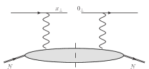
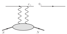
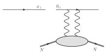
$(a)$	$(b)$	$(c)$

Figure 1: The three different types of interactions of a quark and a nucleus: inelastic (a), elastic in the amplitude (b) and elastic in the complex-conjugate amplitude (c). This illustrates the 3 terms in the r.h.s. of Eq. (5).

The state $N$ in the figure is that of a single nucleon in the nucleus while the $x_{+}$ and $x_{+}^{\prime}$ integrals in Eq. (5) go over the extent of the nucleus.

In the McLerran-Venugopalan model the quark-nucleon scattering amplitude is purely absorptive so that

$$\langle A|\frac{1}{N_{c}}\text{tr}A_{-}(x_{1\perp},x_{1+})A_{-}(x_{2\perp},x_{2+})|A\rangle\\ =\langle A|\frac{1}{N_{c}}\text{tr}T\left[A_{-}(x_{1\perp},x_{1+})A_{-}(x_{2\perp},x_{2+})\right]|A\rangle$$ (6)

matching onto conventional notations when $x_{\perp}^{2}$ is small

$$\langle A|\frac{1}{N_{c}}\text{tr}\bigg{\{}A_{-}(0_{\perp},x_{+}^{\prime})A_{-}(x_{\perp},x_{+})\\ -\frac{1}{2}A_{-}(x_{\perp},x_{+}^{\prime})A_{-}(x_{\perp},x_{+})-\frac{1}{2}A_{-}(0_{\perp},x_{+}^{\prime})A_{-}(0_{\perp},x_{+})\bigg{\}}|A\rangle\\ =-\frac{\pi}{8N_{c}}x_{\perp}^{2}\rho\,xG(x,1/x_{\perp}^{2})\frac{1}{\sqrt{2}}\delta(x_{+}-x_{+}^{\prime})$$ (7)

so that

$$S_{1}=-\frac{x_{\perp}^{2}Q_{s}^{2}}{4}$$ (8)

with

$$Q_{s}^{2}=\frac{4\pi^{2}\alpha C_{F}}{N_{c}^{2}-1}L\rho\,xG(x,1/x_{\perp}^{2})$$ (9)

and where $Q_{s}$ is the quark saturation momentum and $\rho$ the density of nucleons in the nucleus. $L$ is the path length of nuclear matter at the impact parameter at which the quark passes through the nucleus.

Using Eq. (8) in Eq. (4) gives the relation

$$S(x_{\perp})=e^{-x_{\perp}^{2}Q_{s}^{2}/4}$$ (10)

which is recognized as the elastic $S$-matrix for a quark-antiquark dipole passing through the nucleus. Using Eq. (10) in Eq. (1) tells us that the distribution of transverse momenta that a quark picks up in passing through a nucleus is simply related, by Fourier transform, to the elastic dipole-nucleus $S$-matrix element. If one integrates $dN/d^{2}p$ over all transverse momenta the result must be 1,

$$\int d^{2}p_{\perp}\frac{dN}{d^{2}p_{\perp}}=1$$ (11)

since the quark must pick up some value of the transverse momentum. In Eq. (1) this relationship corresponds to $S(0_{\perp})=1$. From Eq. (2) $S(0_{\perp})=1$ corresponds to the unitarity of the operator $V_{0_{\perp}}$ while from Eq. (10) it corresponds to color transparency. But color transparency is a property of gauge theories. Thus the relationships that we are investigating will not be true in a general field theory but are specific to gauge theories. Finally, we have obtained Eq. (10) assuming that the dipole-nucleus scattering amplitude is purely absorptive. While this is natural in the McLerran-Venugopalan model, where the cross-section has no energy dependence, the assumption is not necessary as the second and third terms on the right-hand side of Eq. (5) combine to give an absorptive part in contrast to the individual terms which are time-ordered.

2.2 $p_{\perp}$-broadening more generally

We now turn to a more general discussion of the possible relationship between $p_{\perp}$-broadening and dipole scattering. We shall restrict our discussion to the case where gluons giving quantum contributions to $p_{\perp}$-broadening have a longitudinal momentum much less than that of the quark, thus allowing the quark motion to be given by a Wilson line with a straight line trajectory. This restriction should not limit our ability to investigate and compare the energy evolution of $p_{\perp}$-broadening with that of dipole scattering. A complete study of $p_{\perp}$-broadening vs dipole scattering would require an understanding of how to include the high-momentum gluons into (evolution-independent) impact factors and is beyond our present aim.

Equation (1) is general but, when quantum gluon corrections are included, Eq. (2) should be changed to

$$\tilde{S}(x_{\perp})=\frac{1}{N_{c}}\sum_{n}\text{tr}\bigg{\{}\langle n|T\left(V_{0_{\perp}}e^{i\int d^{4}y{\cal L}_{I}(y)}\right)|A\rangle^{*}\langle n|T\left(V_{x_{\perp}}e^{i\int d^{4}y{\cal L}_{I}(y)}\right)|A\rangle\bigg{\}},$$ (12)

where ${\cal L}_{I}$ is the QCD interaction Lagrangian, say in the lightcone gauge. $S(x_{\perp})$ now has an energy dependence which, for simplicity, we suppress. Using completeness of the states $|n\rangle$, which now include arbitrary numbers of quarks and gluons, in addition to nuclear break-up, one can write Eq. (12) as

$$\tilde{S}(x_{\perp})=\frac{1}{N_{c}}\text{tr}\langle A|\bar{T}\left(V_{0_{\perp}}^{\dagger}e^{-i\int d^{4}y{\cal L}_{I}(y)}\right)T\left(V_{x_{\perp}}e^{i\int d^{4}y{\cal L}_{I}(y)}\right)|A\rangle.$$ (13)

On the other hand, the $S$-matrix for dipole-nucleus scattering is

$$S(x_{\perp})=\frac{1}{N_{c}}\text{tr}\langle A|T\left(V_{0_{\perp}}^{\dagger}V_{x_{\perp}}e^{i\int d^{4}y{\cal L}_{I}(y)}\right)|A\rangle.$$ (14)

Equation (14) is given as a conventional time-ordered product while Eq. (13) is a time-ordered product in a Keldysh-Schwinger [17, 18] sense where the vertices in the $T()$, the second factor in the matrix element in (13), occur in the upper $(x_{1+})$ part of the time contour

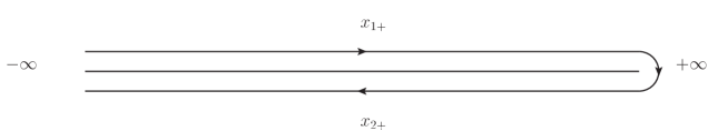
Figure 2: Keldysh-Schwinger contour.

illustrated in Fig. 2, while the vertices in $\bar{T}()$, the first factor in the matrix element in Eq. (13), occur on the lower $(x_{2+})$ part of the time contour.Feynman lines connecting points on the $x_{1+}$-contour have ordinary $i\varepsilon$ factors, lines connecting points on the $x_{2+}$ part of the contour have the sign of it changed, corresponding to the anti-time-ordering indicated in Eq. (13). Feynman lines connecting points on the $x_{1+}$ part of the contour to points on the $x_{2+}$ part of the contour are put on shell.

$\tilde{S}$ and $S$ given by Eq. (13) and (14) respectively will not in general be the same. However, Kovchegov and Tuchin have shown [12] (see Ref. [20] for a broader review, see also Ref. [21]) that the $x$-evolution (energy evolution) of production cross sections is the same as dipole scattering at the leading logarithmic level. Our goal in this paper is to show that this equality persists through next-to-leading order in $x$-evolution.

Finally, we note that (13) can be obtained as a particular discontinuity of an analytically continued Feynman amplitude. To see this we must keep track also of longitudinal momenta of the initial and final quarks as illustrated for the amplitude $A$ in Fig. 3.

Figure 3: The Feynman amplitude described by Eq. (15).

$P$ is the momentum of the target nucleus with $p$ and $p^{\prime}$ the momenta of the quark. One can view $A$ as having the following dependence:

$$A=A\left((p+P)^{2},(p-p^{\prime}+P)^{2},(p_{\perp}-p^{\prime}_{\perp})^{2}\right).$$ (15)

Then

$$1-\tilde{S}=\frac{1}{2i}\text{disc}_{(p-p^{\prime}+P)^{2}}A,$$ (16)

as illustrated in Fig. 4.

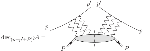
Figure 4: Graphical illustration of the r.h.s. of Eq. (16).

$A$ can be viewed as a dipole scattering amplitude, as shown in Fig. 5,

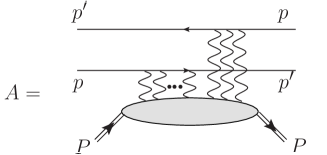
Figure 5: Amplitude $A$ of Fig. 3 viewed as a dipole scattering amplitude.

with the quark and the antiquark momenta, $(p,p^{\prime})$ and $(p^{\prime},p)$ respectively, given by

$$\begin{split}p&=(p_{0},p_{x},p_{y},p_{z})=(p,0,0,p)\\ p^{\prime}&=(\sqrt{(p^{\prime})^{2}+(p^{\prime}_{\perp})^{2}},p_{\perp},p^{\prime}).\end{split}$$ (17)

The arrows on the quark lines in Fig. 5 refer to the flow of baryon number while the momenta are all directed to the right. The discontinuity in Eq. (16) is not just the imaginary part of the dipole scattering so that, in general, one cannot expect a simple relationship between the dipole scattering in Fig. 5 and the particular discontinuity illustrated in Fig. 4.

3 Leading-order calculation

In this section, we review the correspondence between the evolution of $p_{\perp}$-broadening amplitudes and dipole cross sections at leading order. Our aim is also to introduce the basic formalism and conventions that will be used for all calculations throughout this paper.

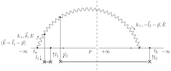
Figure 6: Graph contributing to the leading-order $p_{\perp}$-broadening amplitude. The freed gluon is emitted in the initial state in the amplitude and in the final state in the complex-conjugate amplitude. At the level of the nucleus, we chose one elastic interaction (momentum transfer $l_{1}$) and one inelastic one (momentum transfer $l_{2}$). The exchanged gluons are drawn as dotted lines in order to simplify the graph.

Let us explain the method to evaluate a given lightcone perturbation theory graph such as the one shown in Fig. 6. There are essentially four elements: the product of the energy denominators $D$, the vertex factors, the gluon polarization tensors, and the overall integration.

In order to compute the energy denominators, we first assign a lightcone time $t$ to each vertex. We then evaluate $D$ using the following formula:

$$D=\int\Pi\left[dt\,e^{i(E_{\text{outgoing}}-E_{\text{incoming}})t\pm\varepsilon t}\right],$$ (18)

where the product goes over all vertices and the integration takes into account the ordering of the different times. $\varepsilon$ is a small positive parameter (with dimensions of an energy) that acts as an adiabatic regulator: It is set to zero at the end of the calculation. The sign in front of it is chosen in order to insure the convergence of the corresponding time integral at (plus or minus) infinity, depending whether the considered vertex is in the initial or in the final state. The energy of a state is the sum of the energies of all the particles in the state. The energy $E$ of a particle of 4-momentum $p=(p_{+},p_{-},\vec{p})$ reads

$$E=\frac{\vec{p}^{2}}{2p_{+}}.$$ (19)

The quark-gluon vertices are evaluated in the eikonal approximation throughout this paper. For incoming/outgoing fermions of helicities $\alpha$, $\alpha^{\prime}$, colors $a$, $b$, momentum $p$, and a gluon which carries the Lorentz index $\mu$ and the color $C$, the vertex is represented by the factor

$$\pm 2igt_{ba}^{C}p_{\mu}\delta^{\alpha\alpha^{\prime}},$$ (20)

where the sign is $+$ for a quark and $-$ for an antiquark. The triple-gluon vertices which couple the gluons in the wave function with the nucleus will also have to be evaluated in the eikonal approximation. When the fast gluon line carries the Lorentz indices $\alpha$, $\beta$, the colors $A$, $B$, and the momentum $p$, the vertex factor reads

$$2gf_{ABC}p_{\gamma}g_{\alpha\beta}.$$ (21)

The triple-gluon vertex must however be computed exactly when it appears in the quantum evolution of the wave functions. For incoming momenta $p_{1}$, $p_{2}$ and $p_{3}$ ordered counterclockwise with respective Lorentz indices $\alpha$, $\beta$ and $\gamma$ and color indices $A$, $B$ and $C$, the corresponding vertex factor reads

$$gf_{ABC}\left[g_{\alpha\gamma}(p_{3}-p_{1})_{\beta}+g_{\beta\alpha}(p_{1}-p_{2})_{\gamma}+g_{\gamma\beta}(p_{2}-p_{3})_{\alpha}\right](2\pi)^{3}\delta^{3}(p_{1}+p_{2}+p_{3}).$$ (22)

At next-to-leading order accuracy, we will never need to consider four-gluon vertices.

In addition, each leg of vertex through which the momentum $p$ flows has a factor

$$\frac{1}{\sqrt{2p_{+}}}.$$ (23)

The components of the polarization tensor for the gluon are of 3 different types. For a gluon of momentum $p=(p_{+},p_{-},p_{1},p_{2})$, the latter read

$$d_{--}(p)=\frac{\vec{p}^{2}}{p_{+}^{2}}\ ,\ d_{-i}(p)=\frac{p_{i}}{p_{+}}\ ,\ d_{ij}(p)=-g_{ij}=\delta_{ij}\ \ (i=1,2).$$ (24)

An integration over all $+$ and $\perp$ components of the loop momenta may then be performed, although, as we will discover, a momentum-by-momentum identification holds for some classes of graphs. The integration over the on-shell momentum $k$ is performed as

$$\int\frac{{dk_{+}}d^{2}\vec{k}}{(2\pi)^{3}}.$$ (25)

We are now ready to address the calculation of the diagram depicted in Fig. 6. We interpret it as the representation of a $T$-product, like all other diagrams in this work. Using Eq. (18), we find that the energy denominators read

$$D=\frac{1}{E\bar{E}},$$ (26)

where $E=(\vec{l}_{1}-\vec{p})^{2}/(2k_{+})$, $\bar{E}=(\vec{l}_{2}+\vec{p})^{2}/(2k_{+})$, while the polarizations read

$$\sum_{ij}d_{-i}(l_{1}-p)\cdot d_{ij}\cdot d_{j-}(-l_{2}-p)=\frac{(\vec{p}-\vec{l}_{1})\cdot(\vec{p}+\vec{l}_{2})}{k_{+}^{2}}.$$ (27)

Including the vertex factors, we get, averaging over the quark color and helicity:

$$\frac{1}{2}g^{6}N_{c}^{2}C_{F}\frac{(\vec{p}-\vec{l}_{1})\cdot(\vec{p}+\vec{l}_{2})}{(\vec{p}-\vec{l}_{1})^{2}(\vec{p}+\vec{l}_{2})^{2}}\frac{1}{k_{+}}\ ,$$ (28)

where $C_{F}=(N_{c}^{2}-1)/(2N_{c})$. The transverse momentum conservation is enforced with the help of the additional factor $\delta^{2}(\vec{k}+\vec{p}-\vec{l}_{1})$.

From the $T$-product, we may compute the contribution of the particular graph represented in Fig. 6 to the distribution of transverse momenta of the quark. To this aim, we need to integrate over the 3-momentum of the gluon $k$ and to convolute with appropriate unintegrated gluon distributions which appear in the description of the scattering with the nucleus. The factor which comes with each two-gluon exchange with a particular nucleon in the nucleus involving the transfer of the momentum $l$ reads

$$\pm\int\frac{d^{2}\vec{l}}{\vec{l}^{2}}\frac{xg(x,\vec{l}^{2})}{N_{c}^{2}-1}\rho L$$ (29)

where the sign is $+1$ if the nucleon scatters elastically and $-1$ if it scatters inelastically. When the exchanged gluons attach to the same (quark or gluon) line, a combinatorial factor $\frac{1}{2}$ must be taken into account. Another overall combinatorial factor takes care of the time ordering of the scatterings off the different nucleons. (For the particular graph in Fig. 6, none of these factors is needed). All in all, we get:

$$\left.\frac{dN}{d^{2}p}\right|_{\text{\scriptsize graph in Fig.~{}\ref{lo_labeled}}}=-\frac{\alpha_{s}N_{c}}{N_{c}^{2}-1}\int_{0}^{+\infty}\frac{dk_{+}}{k_{+}}\\ \times\int\frac{d^{2}\vec{l}_{1}}{\vec{l}_{1}^{2}}\frac{d^{2}\vec{l}_{2}}{\vec{l}_{2}^{2}}\frac{(\vec{p}-\vec{l}_{1})\cdot(\vec{p}+\vec{l}_{2})}{(\vec{p}-\vec{l}_{1})^{2}(\vec{p}+\vec{l}_{2})^{2}}\\ \times\left[\alpha_{s}xg(x,\vec{l}_{1}^{2})\rho L\right]\left[\alpha_{s}xg(x,\vec{l}_{2}^{2})\rho L\right].$$ (30)

A priori, we need to sum over any combination of elastic and inelastic exchanges. Actually, they would all look like the ones shown in Fig. 6 and bring factors which are identical in the $p_{\perp}$-broadening case and in the dipole case. Hence it is enough to consider a small number of scatterings: We need only make sure that the case we single out be sufficiently general.

We can compute in the same way the dipole graph in Fig. 7.

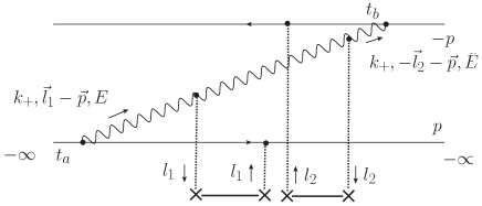
Figure 7: Graph contributing to the lowest-order quantum correction to the dipole forward scattering amplitude. Here there are 2 dipoles interacting with the target nucleus. This graph corresponds to the $p_{\perp}$-broadening graph in Fig. 6.

The only differences with respect to the previous case are: (i) the energy denominators come with a minus sign, (ii) the antiquark-gluon vertices have opposite sign with respect to the quark-gluon vertices and (iii) the scatterings with the nucleus all come with an overall “+” sign in Eq. (29). All the extra minus signs compensate, and we find an exact momentum-by-momentum identity between the expressions for the graphs of Fig. 6 and 7.

We see that we may adopt the following rule as for the relative signs between $p_{\perp}$-broadening amplitudes and dipole amplitudes: Since the extra minus sign which comes from the gluons attaching to the antiquarks is compensated by the change of sign of the discontinuity of the scattering with the nucleus when one goes from $p_{\perp}$ broadening to dipoles, it is enough to take into account only the extra minus signs stemming from the couplings of the gluons in the wave functions to the antiquark.

We have seen in detail how the particular graphs in Fig. 6 and 7 are related. We need to extend the discussion to all possible graphs. First, we note that the $p_{\perp}$-broadening graphs in which the gluon is not produced in the final state trivially correspond to dipole graphs for which the quark or the antiquark is a spectator. So we shall not discuss this case. As for the form of the interaction with the target, we choose to consider one elastic and one inelastic scattering. The gives the most general momentum flow, and since all vertices are eikonal, it would be straightforward to extend the discussion to any form of the scattering.

In the case of $p_{\perp}$-broadening, there are four different nontrivial graphs, depending on whether the gluon is emitted after or before the time of the interaction, in the amplitude and in the complex conjugate amplitude. They are depicted in Fig. 8. The full set of dipole graphs at leading order is represented in Fig. 9.

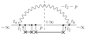
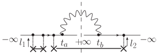
$a$	$b$
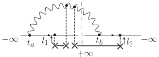
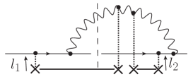
$c$	$d$

Figure 8: Full set of the lowest-order corrections to the $p_{\perp}$-broadening amplitude. Graph $c$ is the one already represented in Fig. 6, and graph $d$ has the same expression since it is related by a simple symmetry.

We have computed graph $c$ (Fig. 6 and 8) and shown that its expression is the same as the expression for the dipole graph $\gamma$ (Fig. 7 and 9). Graph $d$ is similar to $c$ and it is straightforward to check that its expression is the same as the expression for the dipole graph in which the gluon attaches to the antiquark in the amplitude and to the quark in the complex conjugate amplitude. In other words,

$$c=\gamma\ \ \text{and}\ \ d=\delta.$$ (31)

We turn to graph $a$ in Fig. 8. The scattering occurs after the emission of the gluon both in the amplitude and in the complex conjugate amplitude. The gluons exchanged with the nucleus may be chosen to scatter with the quark line only: It is easy to check that the graphs in which the fast gluon scatters cancel between each other. The polarization factor for the gluon is then $d_{--}(-l_{2}-p)$. We keep two scatterings with the quark, one elastic and one inelastic. Leaving out the factors describing the interaction with the target and the integration over $k_{+}$, the expression for the graph reads (compare to Eq. (28))

$$a=-2g^{6}C_{F}^{3}\frac{1}{(\vec{p}+\vec{l}_{2})^{2}}\frac{1}{k_{+}}.$$ (32)

The corresponding dipole graphs would be $\alpha$, $\alpha^{\prime}$, $\beta$ and $\beta^{\prime}$ in Fig. 9. We see that these graphs are purely virtual: Therefore, for the correspondence to work, it is crucial that all interactions with the nucleus happen with the quarks and not with the gluon in the $p_{\perp}$-broadening case, which is effectively verified since scatterings with the gluons cancel among themselves.

For this process, there are also graphs with instantaneous gluon exchanges (graphs $\alpha^{\prime}$ and $\beta^{\prime}$). We take them into account by modifying the $d_{--}$ component of the polarization tensor in the corresponding causal graphs ($\alpha$ and $\beta$ resp.) as follows [14]:

$$d_{--}(k)\rightarrow d_{--}(k)\left(1-\frac{\Sigma}{E_{\text{gluon}}}\right)\equiv d_{--}(k)\times F\ ,$$ (33)

where $E_{\text{gluon}}$ is the energy carried by the gluon, and $\Sigma$ is the factor in the energy denominators associated to the emission of this gluon. The second equality defines the $F$-factor. Since the graphs containing gluons which are exchanged instantaneously may be effectively taken into account through the above modification in the expressions of the causal graphs, we will not draw them systematically in the following sections. We shall just perform the substitution (33) whenever the kinematics allow for instantaneous exchanges.

Let us evaluate the dipole graph $\alpha$ in Fig. 9. The energy denominators read

$$D=\frac{1}{2i\varepsilon(\bar{E}-i\varepsilon)}\ ,$$ (34)

where $\bar{E}=(\vec{p}+\vec{l}_{2})^{2}/(2k_{+})$. The divergence encoded in the $1/\varepsilon$ singularity may be traced to the absence of time scale for the exchange of the gluon between the quark and the antiquark, making it equally likely for all times between $t=-\infty$ and $t=0$. The expression for this graph reads, before integration over the momenta,

$$\alpha=-\frac{1}{2}g^{6}C_{F}^{3}\frac{(\vec{p}+\vec{l}_{2})^{2}}{k_{+}^{3}}\frac{1}{2i\varepsilon}\frac{1}{\bar{E}-i\varepsilon}\ ,$$ (35)

and hence this graph gives a divergent contribution. Adding graph $\alpha^{\prime}$ turns out to cancel the divergence (a fact which has already been noticed by Kovchegov [23]). To take to latter into account, we multiply $\alpha$ by the factor $F$ defined in Eq. (33), the energy of the gluon being $\bar{E}$, and $\Sigma\equiv\bar{E}-i\varepsilon$:

$$F_{\alpha}=1-\frac{\bar{E}-i\varepsilon}{\bar{E}}=\frac{i\varepsilon}{\bar{E}}.$$ (36)

The sum of the graphs $\alpha$ and $\alpha^{\prime}$ reads

$$\alpha+\alpha^{\prime}=-g^{6}C_{F}^{3}\frac{1}{(\vec{p}+\vec{l}_{2})^{2}}\frac{1}{k_{+}},$$ (37)

which is now finite. The sum of the graphs $\beta+\beta^{\prime}$ has exactly the same expression. Comparing to Eq. (32), we see that the following identity holds:

$$a=\alpha+\alpha^{\prime}+\beta+\beta^{\prime}.$$ (38)

The purely final state graph $b$ corresponds, as we may check by explicit calculation, to the complex conjugate graphs:

$$b=\bar{\alpha}+\bar{\alpha}^{\prime}+\bar{\beta}+\bar{\beta}^{\prime}.$$ (39)

This completes the proof that at leading logarithmic order, the evolution kernel of the $p_{\perp}$-broadening amplitude is identical to the evolution kernel of the dipole $S$-matrix.

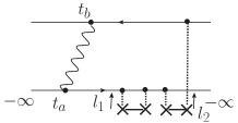
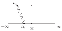
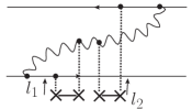
$\alpha$	$\beta$	$\gamma$
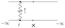
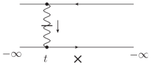
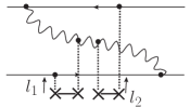
$\alpha^{\prime}$	$\beta^{\prime}$	$\delta$

Figure 9: Set of leading-order virtual (left) and real (right) corrections to the dipole amplitude. In the graphs $\alpha$ and $\beta$, the exchanged gluon is causal, whereas in $\alpha^{\prime}$ and $\beta^{\prime}$, it is exchanged instantaneously. Graph $\gamma$ is equivalent to the graph in Fig. 7, and $\delta$ has the same expression.

4 Proof of the equivalence at next-to-leading order

We consider systematically all relevant graphs in the view of proving the equivalence of the evolution kernels at next-to-leading order, namely, that the identity (1) is preserved by the energy evolution at that accuracy. Therefore, we keep treating the quark-gluon vertices in the eikonal approximation, but the triple gluon vertices which contribute to the evolution kernel are computed exactly.

We classify the graphs according to the number of quark-gluon vertices. There are two, three of four such vertices. In the first case, the diagrams contain a gluon loop, but it turns out that we do not need to evaluate it explicitly to prove the equivalence. In the second case instead, the three-gluon vertex has to be computed and the different gluon polarizations fully discussed. Furthermore, we find that a momentum-by-momentum identification no longer holds, and the identification results from an analytical continuation of the integration over the longitudinal component of the momenta. Finally, in the third case, the classes of diagrams that have to be considered together for the identification to happen are larger. Moreover, while it is enough to analyze the energy denominators in order to prove the equivalence, which makes each calculation quite easy, the graphs are numerous, and analytical continuation is also needed for some diagrams.

4.1 Two quark-gluon vertices

We will first analyze the $p_{\perp}$-broadening graphs, then the dipole graphs, and the comparison will be drawn in the last subsection.

4.1.1 $p_{\perp}$-broadening graphs

With two quark-gluon vertices exactly, the next-to-leading order graphs contain a gluon loop. One such graph contributing to $p_{\perp}$ broadening is represented in Fig. 10.

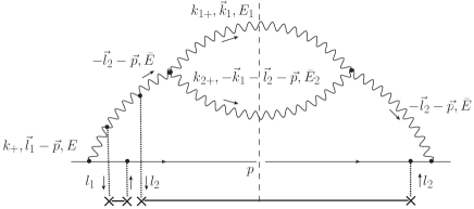
Figure 10: One particular graph contributing to $p_{\perp}$-broadening at next-to-leading order and exhibiting two quark-gluon vertices exactly, as far as quantum evolution is concerned, with one elastic and one inelastic interaction with the target. The energies and momenta of the particles are labeled explicitly.

The other graphs only differ from that one by the chronology of the interactions.

Hence we group the graphs according to the time at which the quark-gluon and gluon-gluon branchings occur, in the amplitude and in the complex conjugate amplitude, relatively to the time at which the interaction with the target nucleus occurs. Each such class of (nonvanishing) $p_{\perp}$-broadening graphs corresponds to a particular set of dipole graphs, which we will discuss in Sec. 4.1.2 after having reviewed all $p_{\perp}$-broadening graphs.

We anticipate the fact that the only nontrivial factors to compare between the contribution of a given set of $p_{\perp}$-broadening graphs and of dipole graphs are the energy denominators: One may therefore avoid the discussion of the gluon loop.

We shall name the $p_{\perp}$-broadening graphs with the help of the ordering of their vertices with respect to the scattering. For example ${\text{IF}\overline{\text{IF}}}$ (Fig. 11) means one $qg$ vertex at early times and one 3-gluon vertex at late times in the amplitude (left of the cut), and the same in the complex-conjugate amplitude (right of the cut).

Both quark-gluon vertices in the initial state.

Let us first consider the case in which the $qg$ branchings are in the initial state both in the amplitude and in the complex conjugate amplitude (namely the $qg$ vertices occur at negative times). The $gg$ vertices may then occur either at positive or negative times.

The first case we examine is when the $gg$ branchings both occur in the final state. The full set of graphs is shown in Fig. 11.

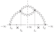
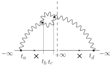
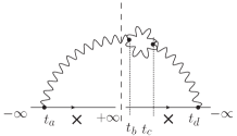
${\text{IF}\overline{\text{IF}}}$	${\text{IFF}\overline{\text{I}}}$	${\text{I}\overline{\text{IFF}}}$

Figure 11: Complete set of graphs for which the $qg$ vertices are in the initial state and the 3-gluon vertices in the final state. The interactions with the nucleus are understood since they are the same as in Fig. 10 for all three graphs.

We see that we can label all momenta exactly as in Fig. 10 since the topology of all the graphs is the same. Therefore the expressions for these graphs will differ only in the energy denominators. Let us evaluate the latter using Eq. (18).

We label the time at the branchings as $t_{a}<t_{b}$ for the $qg$ and $gg$ branchings in the amplitude respectively, and $t_{d}<t_{c}$ for the same branchings in the complex conjugate amplitude. The energy denominators corresponding to the graph in Fig. 10 (or equivalently the leftmost graph in Fig. 11) are obtained from the evaluation of the following integral (see Eq. 18):

$$D_{{\text{IF}\overline{\text{IF}}}}=\int_{-\infty}^{0}dt_{a}\int_{0}^{+\infty}dt_{b}\int_{+\infty}^{0}dt_{c}\int_{0}^{-\infty}dt_{d}\,\\ \exp\left\{i\left[Et_{a}+(E_{1}+\bar{E}_{2}-\bar{E})(t_{b}-t_{c})-\bar{E}t_{d}\right]+\varepsilon(t_{a}-t_{b}-t_{c}+t_{d})\right\}.$$ (40)

We have defined (see Fig. 10)

$$E=\frac{(\vec{p}-\vec{l}_{1})^{2}}{2k_{+}},\ \bar{E}=\frac{(\vec{p}+\vec{l}_{2})^{2}}{2k_{+}},\ E_{1}=\frac{\vec{k}_{1}^{2}}{2k_{1+}},\ \bar{E}_{2}=\frac{(\vec{k}_{1}+\vec{l}_{2}+\vec{p})^{2}}{2k_{2+}},$$ (41)

and from the conservation of the longitudinal momentum, $k_{2+}=k_{+}-k_{1+}$. (Of course, the “bar” does not mean complex conjugate in these equations). The result of the integrations over the different times reads

$$D_{{{\text{IF}\overline{\text{IF}}}}}=\frac{1}{E\bar{E}\left(E_{1}+\bar{E}_{2}-\bar{E}\right)^{2}}.$$ (42)

We perform a similar calculation for the two other graphs in this group. The one in which the loop is in the amplitude (Fig. 11, middle) has the following energy denominators, after expansion for $\varepsilon\rightarrow 0$:

$$D_{{{\text{IFF}\overline{\text{I}}}}}=-\frac{1}{2i\varepsilon}\frac{1}{E\bar{E}\left(E_{1}+\bar{E}_{2}-\bar{E}\right)}-\frac{1}{2}\bigg{[}\frac{1}{E\bar{E}\left(E_{1}+\bar{E}_{2}-\bar{E}\right)^{2}}\\ +\frac{1}{E^{2}\bar{E}\left(E_{1}+\bar{E}_{2}-\bar{E}\right)}-\frac{1}{E\bar{E}^{2}\left(E_{1}+\bar{E}_{2}-\bar{E}\right)}\bigg{]}.$$ (43)

This time, there is a divergent term when $\varepsilon\rightarrow 0$, which is however imaginary. The graph in which the loop is in the complex conjugate amplitude has a similar expression up to sign changes, in such a way that in the sum $D_{{{\text{IFF}\overline{\text{I}}}}}+D_{{{\text{I}\overline{\text{IFF}}}}}$, the divergent imaginary part cancels as well as the two last terms in Eq. (43) while the second term gains a factor 2. The sum of the 3 denominators then cancels,

$$D_{{{\text{IF}\overline{\text{IF}}}}}+D_{{{\text{IFF}\overline{\text{I}}}}}+D_{{{\text{I}\overline{\text{IFF}}}}}=0,$$ (44)

and therefore, the total contribution of these graphs is zero.

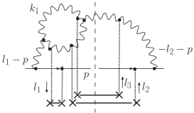
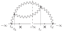
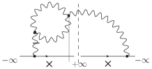
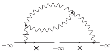
${\text{IIF}\overline{\text{I}}}$	${\text{II}\overline{\text{IF}}}$

Figure 12: Graphs in which the two quark-gluon vertices are in the initial state, one 3-gluon vertex is in the initial state in the amplitude, and the other one is in the final state, either in the amplitude or in the complex-conjugate amplitude. This set should be supplemented with the symmetric ones, obtained by taking the complex conjugate.

Let us turn to the case in which the leftmost $gg$ branching occurs before the time of the scattering in the amplitude while the rightmost one occurs in the final state, either in the amplitude or in the complex conjugate amplitude. Then there are the four diagrams depicted in Fig. 12. The Lorentz structure is the same for the graphs ${\text{IIF}\overline{\text{I}}}$ and ${\text{II}\overline{\text{IF}}}$. We evaluate the energy denominators of the causal graphs (first row in Fig. 12) as

$$D_{{\text{IIF}\overline{\text{I}}}}=\frac{1}{E\bar{E}(E_{1}+E_{2})(E_{1}^{\prime}+\bar{E}^{\prime}_{2}-\bar{E}^{\prime})},$$ (45)

where

$$E_{2}=\frac{(\vec{p}-\vec{l}_{1}+\vec{k}_{1})^{2}}{2k_{2+}},\ E_{1}^{\prime}=\frac{(\vec{k}_{1}-\vec{l}_{3})^{2}}{2k_{1+}},\ \bar{E}_{2}^{\prime}=\frac{(\vec{p}+\vec{k}_{1}+\vec{l}_{2})^{2}}{2k_{2+}},\ \bar{E}^{\prime}=\frac{(\vec{p}+\vec{l}_{2}+\vec{l}_{3})^{2}}{2k_{+}},$$ (46)

see Fig. 12. Computing in the same way $D_{{\text{II}\overline{\text{IF}}}}$, we find that $D_{{\text{II}\overline{\text{IF}}}}=-D_{{\text{IIF}\overline{\text{I}}}}$. Since all other factors are the same for these graphs, their sum cancels, independently for each polarization of the gluons.

When the polarization $(--)$ is chosen for the leftmost gluon in ${\text{IIF}\overline{\text{I}}}$ and ${\text{II}\overline{\text{IF}}}$, then each of these graphs also cancels with the same graphs where the latter gluon is exchanged instantaneously (graphs in the second row in Fig. 12). Indeed, according to the rule (33), the polarization tensor $d_{--}$ for this gluon has to be multiplied by the factor

$$F_{{\text{IIF}\overline{\text{I}}},{\text{II}\overline{\text{IF}}}}\equiv 1-\frac{E-i\varepsilon}{E}=\frac{i\varepsilon}{E}.$$ (47)

The product of this factor with the corresponding energy denominators vanishes since $D_{{\text{IIF}\overline{\text{I}}},{\text{II}\overline{\text{IF}}}}$ are finite for $\varepsilon\rightarrow 0$. So there is no global contribution of the instantaneous-exchange graphs either.

So far, we have not found any contribution to $p_{\perp}$-broadening of the graphs that we have examined. We turn to the last class of graphs in which both three-gluon vertices are in the initial state, either in the amplitude or in the complex-conjugate amplitude. Again in this case, as for the leading-order graph $a$ in Fig. 8, all graphs in which one of the gluons in the wave functions scatters with the nucleus cancel among themselves. The complete set of graphs in which the gluons are causal is shown in Fig. 13.

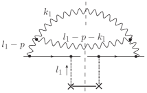
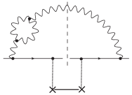
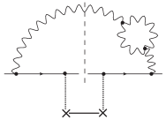
${\text{II}\overline{\text{II}}}$	${\text{III}\overline{\text{I}}}$	${\text{I}\overline{\text{III}}}$

Figure 13: Causal graphs in which all vertices are in the initial state. The scattering with the target occurs with the quark: Graphs in which one of the gluons scatters cancel among each other.

There are in addition graphs in which at least one gluon is replaced by a contact interaction, see Fig. 14 and 15.

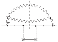
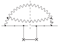
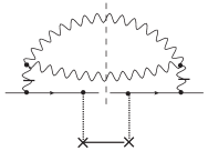
Figure 14: Instantaneous-exchange graphs corresponding to graph ${\text{II}\overline{\text{II}}}$ in Fig. 13. They are effectively taken into account in our calculation by multiplying ${\text{II}\overline{\text{II}}}$ for the longitudinal polarization of the gluons which attach to the quarks by two $F$-factors (see Eq. (33)).

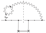
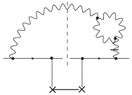
Figure 15: Instantaneous-exchange graphs corresponding to graphs ${\text{III}\overline{\text{I}}}$ and ${\text{I}\overline{\text{III}}}$ in Fig. 13.

Before we proceed to the computation of the energy denominators, we need to discuss the helicity structure of the gluons. The leg of the gluons which attached to the quark always carries the longitudinal polarization “$-$” since the $qg$ vertices are eikonal. The other leg of these gluons is either longitudinally, or transversely polarized. Actually, in these graphs in which no interaction occurs between the gluons in the wave function and the target, the leg which attaches to the loop of both of these gluons must have the same polarization. Hence both gluons come either with a $d_{--}$ or with a $d_{-\perp}$ polarization factor.

In order to easily incorporate the instantaneous-exchange graphs using the modification (33) of $d_{--}$, we will distinguish the two possible polarizations: In the $(-\perp)$ case, it will be enough to consider the sum of the energy denominators of the relevant graphs, while in the $(--)$ case, we will have to weight them by appropriate $F$-factors computed with the help of Eq. (33).

We go back to the graphs of Fig. 13. The energy denominators read

$$D_{{\text{II}\overline{\text{II}}}}=\frac{1}{E^{2}(E_{1}+E_{2})^{2}},\ D_{{\text{III}\overline{\text{I}}}}=D_{{\text{I}\overline{\text{III}}}}=\frac{1}{E^{3}(E_{1}+E_{2})}$$ (48)

The sum of the denominators reads

$$D_{{\text{II}\overline{\text{II}}}}+D_{{\text{III}\overline{\text{I}}}}+D_{{\text{I}\overline{\text{III}}}}=\frac{1}{E^{2}(E_{1}+E_{2})^{2}}+\frac{2}{E^{3}(E_{1}+E_{2})}.$$ (49)

The incorporation of the graphs of Fig. 14 and 15 require to multiply $D_{{\text{III}\overline{\text{I}}}}$ and $D_{{\text{I}\overline{\text{III}}}}$ by

$$F_{{\text{III}\overline{\text{I}}}}=1-\frac{E-i\varepsilon}{E}=\frac{i\varepsilon}{E}\ ,\ \ F_{{\text{I}\overline{\text{III}}}}=-\frac{i\varepsilon}{E}$$ (50)

and $D_{{\text{II}\overline{\text{II}}}}$ by $F_{{\text{III}\overline{\text{I}}}}\times F_{{\text{I}\overline{\text{III}}}}$. So because of the finiteness of the energy denominators, once we add the instantaneous-exchange graphs, the contribution of the $(--)$ polarization vanishes.

Both quark-gluon vertices in the final state.

There are 3 causal graphs in which the gluon is emitted off the quark at late times both in the amplitude and in the complex conjugate amplitude. They are represented in Fig. 16. Since the kinematics is the same for all these graphs, it is again enough to address the energy denominators.

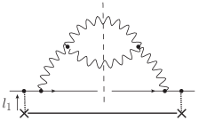
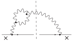
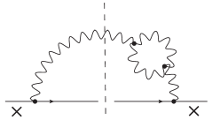
${\text{FF}\overline{\text{FF}}}$	${\text{FFF}\overline{\text{F}}}$	${\text{F}\overline{\text{FFF}}}$

Figure 16: Set of the causal graphs in which all vertices are in the final state. One should also consider the graphs where some gluons are exchanged instantaneously: We do not show them since they look exactly like those of Fig. 14 and 15.

They read

$$\begin{split}D_{{\text{FF}\overline{\text{FF}}}}&=\frac{1}{(E_{1}+E_{2})^{2}\left(E_{1}+E_{2}-E\right)^{2}}\\ D_{{\text{FFF}\overline{\text{F}}}}&=-\frac{1}{2i\varepsilon}\frac{1}{{E}^{2}\left(E_{1}+E_{2}-E\right)}+\frac{1}{{E}^{3}\left(E_{1}+E_{2}-E\right)}\\ &\ \ \ \ -\frac{1}{2}\frac{1}{{E}^{2}\left(E_{1}+E_{2}-E\right)^{2}}\\ D_{{\text{F}\overline{\text{FFF}}}}&=\bar{D}_{{\text{FFF}\overline{\text{F}}}}.\end{split}$$ (51)

After some rearrangements, their sum reduces to

$$D_{{\text{FF}\overline{\text{FF}}}}+D_{{\text{FFF}\overline{\text{F}}}}+D_{{\text{F}\overline{\text{FFF}}}}=\frac{1}{{E}^{2}(E_{1}+E_{2})^{2}}+\frac{2}{{E}^{3}(E_{1}+E_{2})},$$ (52)

namely it is identical to Eq. (49). In order to take into account the instantaneous-exchange graphs, we need to multiply the denominators by the respective factors

$$F_{{\text{FF}\overline{\text{FF}}}}^{2}=\left(\frac{E_{1}+E_{2}}{{E}}\right)^{2},\ F_{{\text{FFF}\overline{\text{F}}}}=1+\frac{2i\varepsilon}{E}\ \ \text{and}\ \ F_{{\text{F}\overline{\text{FFF}}}}=\bar{F}_{{\text{FFF}\overline{\text{F}}}}.$$ (53)

Then we find that the sum of all instantaneous-exchange graphs and of the causal graphs with the $(--)$ polarization for the gluons that couple to the quark has the factor

$$F_{{\text{FF}\overline{\text{FF}}}}^{2}D_{{\text{FF}\overline{\text{FF}}}}+F_{{\text{FFF}\overline{\text{F}}}}D_{{\text{FFF}\overline{\text{F}}}}+F_{{\text{F}\overline{\text{FFF}}}}D_{{\text{F}\overline{\text{FFF}}}}=0,$$ (54)

and hence vanishes.

One $qg$ vertex in the initial state, one in the final state.

The causal graphs are represented in Fig. 17. The energy denominators read

$$D_{{\text{FFF}\overline{\text{I}}}}=-\frac{1}{2i\varepsilon}\frac{1}{E\bar{E}(E-E_{1}-E_{2})}+\frac{1}{2}\frac{1}{E\bar{E}^{2}(E-E_{1}-E_{2})}\\ +\frac{3}{2}\frac{1}{{E}^{2}\bar{E}(E-E_{1}-E_{2})}+\frac{1}{2}\frac{1}{E\bar{E}(E-E_{1}-E_{2})^{2}}$$ (55)

for the leftmost graph,

$$D_{{\text{FF}\overline{\text{IF}}}}=-\frac{1}{\bar{E}(E_{1}+E_{2})(E-E_{1}-E_{2})^{2}}$$ (56)

for the graph in which there are 2 gluons in the final state (graph in the middle in Fig. 17), and

$$D_{{\text{F}\overline{\text{IFF}}}}=\frac{1}{2i\varepsilon}\frac{1}{E\bar{E}(E-E_{1}-E_{2})}-\frac{1}{2}\frac{1}{E\bar{E}^{2}(E-E_{1}-E_{2})}\\ -\frac{1}{2}\frac{1}{{E}^{2}\bar{E}(E-E_{1}-E_{2})}+\frac{1}{2}\frac{1}{E\bar{E}(E-E_{1}-E_{2})^{2}}$$ (57)

for the graph in which the loop is on the right of the cut (rightmost graph in Fig. 17).

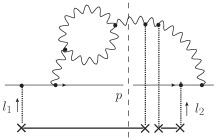
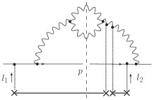
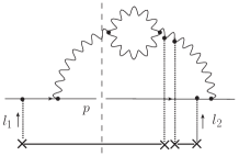
${\text{FFF}\overline{\text{I}}}$	${\text{FF}\overline{\text{IF}}}$	${\text{F}\overline{\text{IFF}}}$

Figure 17: Causal graphs in which one $qg$ vertex is in the initial state, and one in the final state. This list should be completed with the instantaneous-exchange graphs in correspondence with the two leftmost graphs, and with the complex-conjugate ones.

The sum of these denominators reads

$$D_{{\text{FFF}\overline{\text{I}}}}+D_{{\text{FF}\overline{\text{IF}}}}+D_{{\text{F}\overline{\text{IFF}}}}=-\frac{1}{{E}^{2}\bar{E}(E_{1}+E_{2})^{2}}.$$ (58)

The instantaneous-exchange graphs are taken into account with the help of the factors

$$F_{{\text{FFF}\overline{\text{I}}}}=1+\frac{2i\varepsilon}{E},\ F_{{\text{FF}\overline{\text{IF}}}}=\frac{E_{1}+E_{2}}{E}.$$ (59)

Again, the contribution of these graphs summed with the causal graphs which have the $(--)$ polarization vanishes, since

$$F_{{\text{FFF}\overline{\text{I}}}}D_{{\text{FFF}\overline{\text{I}}}}+F_{{\text{FF}\overline{\text{IF}}}}D_{{\text{FF}\overline{\text{IF}}}}+D_{{\text{F}\overline{\text{IFF}}}}=0.$$ (60)

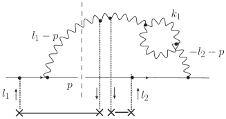
${\text{F}\overline{\text{III}}}$

Figure 18: Causal graph in which one $qg$ vertex is in the initial state, one in the final state, and the gluon loop is fully in the initial state.

The graph in which the gluon loop is in the initial state (Fig. 18) has the following denominators:

$$D_{{\text{F}\overline{\text{III}}}}=-\frac{1}{E\bar{E}^{2}(E_{1}+\bar{E}_{2})}.$$ (61)

The sum of the instantaneous-exchange graph with the $(--)$ polarization in the causal graph once again vanishes.

Finally, we address the graphs in Fig. 19.

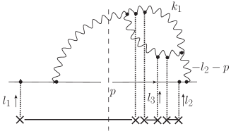
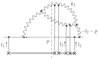
${\text{F}\overline{\text{IIF}}}$	${\text{FF}\overline{\text{II}}}$

Figure 19: Causal graphs in which the gluon loop interacts. There are in addition 2 instantaneous-exchange graphs (not shown).

We find the following energy denominators:

$$\begin{split}D_{{\text{F}\overline{\text{IIF}}}}&=\frac{1}{E\bar{E}(E_{1}+\bar{E}_{2})(E-E_{1}^{\prime\prime}-E_{2}^{\prime\prime})},\\ D_{{\text{FF}\overline{\text{II}}}}&=-\frac{1}{\bar{E}(E_{1}+\bar{E}_{2})(E_{1}^{\prime\prime}+E_{2}^{\prime\prime})(E-E_{1}^{\prime\prime}-E_{2}^{\prime\prime})},\end{split}$$ (62)

where

$$E_{1}^{\prime\prime}=\frac{(\vec{k}_{1}+\vec{l}_{1}+\vec{l}_{3})^{2}}{2k_{1+}},\ E_{2}^{\prime\prime}=\frac{(\vec{p}+\vec{k}_{1}+\vec{l}_{3})^{2}}{2k_{2+}}.$$ (63)

Their sum reads

$$D_{{\text{F}\overline{\text{IIF}}}}+D_{{\text{FF}\overline{\text{II}}}}=-\frac{1}{E\bar{E}(E_{1}+\bar{E}_{2})(E_{1}^{\prime\prime}+E_{2}^{\prime\prime})}.$$ (64)

Again, the sum of the $(--)$ components and of the instantaneous-exchange graphs gives a null contribution, due to the finiteness of the denominators and to the fact that the $F$-factors are of order $\varepsilon$.

4.1.2 Dipole graphs

The full set of nontrivial causal dipole graphs is shown in Fig. 20,21,22, up to graphs deduced from the latter by obvious symmetries. (We do not discuss the graphs in which the gluons both couple to the same quark or antiquark, because the correspondence with $p_{\perp}$-broadening graphs in which the evolution happens entirely either in the amplitude or in the complex-conjugate amplitude is then immediate). We may label the flow of the momenta through the graphs in such a way that it is the same as in the $p_{\perp}$-broadening case. This justifies a posteriori that only the energy denominators need to be compared.

The expression for the energy denominators are very easy to obtain for these graphs.

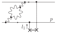
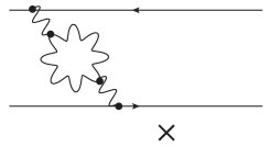
$\alpha_{1}$	$\alpha_{2}$

Figure 20: Virtual graphs (One dipole exactly scatters). There would be 6 additional graphs in which one or both gluons which couple to the quark/antiquark are exchanged instantaneously. $\alpha_{1}$ and $\alpha_{2}$ only differ by the ordening of the $qg$ and $\bar{q}g$ vertices. We do not display the complex-conjugate graphs.

The graphs $\alpha$ in Fig. 20 are virtual graphs, which contribute equally. The energy denominators read

$$D_{\alpha_{1}}+D_{\alpha_{2}}=-\frac{1}{2i\varepsilon}\frac{1}{E^{2}(E_{1}+E_{2})}-\frac{2}{E^{3}(E_{1}+E_{2})}-\frac{1}{E^{2}(E_{1}+E_{2})^{2}},$$ (65)

where $E$, $E_{1}$ $E_{2}$ are defined in the previous section. To compute the sum of the $(--)$ polarization and of the instantaneous-exchange graphs (not drawn), it is enough to multiply the previous denominators by the factor

$$F=\left(1-\frac{E-i\varepsilon}{E}\right)\left(1-\frac{E-3i\varepsilon}{E}\right)\sim\varepsilon^{2},$$ (66)

and thus the latter sum vanishes: The $(--)$ polarization of the gluons does effectively not contribute.

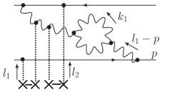
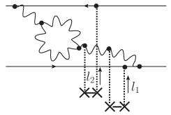
$\beta_{1}$	$\beta_{2}$

Figure 21: Graphs where there are 2 dipoles at the time of the interaction. There would be 2 additional instantaneous-exchange graph, and also the graphs in which the gluon couples to the quark in the amplitude and to the antiquark in the complex-conjugate amplitude (namely the complex-conjugate graphs). The arrows on the gluons indicate the direction of the flow of the transverse momentum.

Similarly, the energy denominators for the graphs of Fig. 21 read

$$D_{\beta_{1}}=\frac{1}{{E}^{2}\bar{E}(E_{1}+E_{2})^{2}},\ D_{\beta_{2}}=\frac{1}{E{\bar{E}}^{2}(E_{1}+\bar{E}_{2})^{2}}.$$ (67)

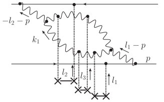
$\gamma$

Figure 22: Graph where there are 3 dipoles at the time of the interaction. In the same manner as for the diagrams of Fig. 20, there would be 3 extra graphs with contact interactions instead of the external causal gluon propagators. There are also the graphs in which the couplings of the gluons to the quark and antiquark are interchanged between the amplitude and the complex-conjugate amplitude.

Last, the graph in Fig. 22 gives

$$D_{\gamma}=\frac{1}{E\bar{E}(E_{1}+\bar{E}_{2})(E_{1}^{\prime\prime}+E_{2}^{\prime\prime})}.$$ (68)

The $F$ factors for the two last classes of graphs are proportional to $\varepsilon$: Hence the $(--)$ polarization components compensate with the instantaneous-exchange graphs also in the two previous cases.

4.1.3 Proof of the correspondence

The identification between the relevant graphs is now quite straightforward.

The nonzero graphs in the case of $p_{\perp}$-broadening are those of Fig. 13, 16, 17,  18, 19 with the $(-\perp)$ polarization for the gluons which hook to the quark. The associated denominators are given in Eq. (49),(52),(58),(61),(64) respectively.

We naturally identify the dipole graphs $\alpha_{1},\alpha_{2}$ of Fig. 20 with the $p_{\perp}$-broadening graphs where all vertices are in the initial state of Fig. 13, since they can be topologically related by bending over the quark line to form the antiquark of the dipole. It is easy to check the formal identity of the expressions for these graphs: The polarization and vertex factors are the same in the $p_{\perp}$-broadening case and in the dipole case, except for a minus sign difference which comes from the $qg$ coupling becoming a $\bar{q}g$ coupling. We notice that we may also choose the interaction with the nucleus to be the same in both cases, and label the momenta in the same way as for $p_{\perp}$-broadening. We see that the following identity between the energy denominators holds:

$$D_{{\text{II}\overline{\text{II}}}}+D_{{\text{III}\overline{\text{I}}}}+D_{{\text{I}\overline{\text{IIII}}}}=-\text{Re}\left(D_{\alpha_{1}}+D_{\alpha_{2}}\right).$$ (69)

The minus sign in the r.h.s. is explained by the coupling to the antiquark. The only remaining mismatch is an imaginary term which cancels when the complex conjugate graphs are taken into account.

Bending over the quark on the right of the cut in the graphs of Fig. 16, we see that we get the symmetric of the dipole graphs of Fig. 20, namely the complex conjugate graphs (not represented). The formal identity between the energy denominators reads

$$D_{{\text{FF}\overline{\text{FF}}}}+D_{{\text{FFF}\overline{\text{F}}}}+D_{{\text{F}\overline{\text{FFF}}}}=-\text{Re}\left(\bar{D}_{\alpha_{1}}+\bar{D}_{\alpha_{2}}\right).$$ (70)

In the same manner, we see that the graphs of Fig. 17 are topologically related to $\beta_{1}$ in Fig. 21, the one in Fig. 18 is related to $\beta_{2}$, and the ones in Fig. 19 look equivalent to $\gamma$ in Fig. 22. As a matter of fact, the following identities are verified:

$$\begin{split}D_{{\text{FFF}\overline{\text{I}}}}+D_{{\text{FF}\overline{\text{IF}}}}+D_{{\text{F}\overline{\text{IFF}}}}&=-D_{\beta_{1}},\\ D_{{\text{F}\overline{\text{III}}}}&=-D_{\beta_{2}},\\ D_{{\text{F}\overline{\text{IIF}}}}+D_{{\text{FF}\overline{\text{II}}}}&=-D_{\gamma}.\end{split}$$ (71)

Equations (69),(70),(71) prove the equivalence of $p_{\perp}$ broadening and dipoles for the considered class of diagrams.

Note that the $p_{\perp}$-broadening graphs which cancel among themselves would not have any dipole counterparts allowed by the kinematics. Indeed, for example the graphs of Fig. 12 would correspond to a dipole graph such as the one shown in Fig. 23, which is forbidden by momentum conservation.

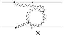
Figure 23: Dipole graph which would correspond to the (vanishing) $p_{\perp}$-broadening graph of Fig. 12, but which is not allowed by momentum conservation.

4.2 Three quark-gluon vertices

We turn to the case in which there are 3 quark-gluon vertices. The NLO graphs all have one 3-gluon vertex (like the one in Fig. 24), see e.g. Fig. 25 for a sample of the $p_{\perp}$-broadening graphs and Fig. 26 for the would-be equivalent dipole graphs.

Let us analyze the Lorentz structure of the upper part of these graphs. The gluons entering the vertex may have “$-$” or “$\perp$” polarizations. It turns out that there are only four possible configurations: Either all gluons are transverse, or one of them (and only one) has a “$-$” polarization. All other possibilities lead to vanishinig contributions. The gluon which is polarized longitudinally may be exchanged instantaneously if the kinematical configuration of the diagram allows it; Such configurations are taken into account by a modification of the corresponding polarization tensor, see Eq. (33).

It is useful to write down the factors specific to the different polarization configurations for the typical graph shown in Fig. 24.

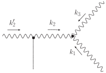
Figure 24: Typical momentum configuration around the 3-gluon vertex. The arrows show the direction of the transverse components of the momenta. The “$+$” components are always directed to the right. The gluons which carry the momenta $k_{1}$ and $k_{3}$ may also be exchanged instantaneously in some graphs, in which case the factors $E_{1}$ and $E_{3}$ which come with the polarization tensors of these gluons (see Tab. 1) are replaced by $E_{1}-\Sigma_{1}$ and $E_{3}-\Sigma_{3}$, where $\Sigma_{1}$ and $\Sigma_{3}$ are the energy denominators of the corresponding causal graphs.

All other configurations of the momenta may be deduced from the one illustrated in Fig. 24 by appropriate changes in the signs. Note that we will keep the transverse momenta always incoming to the 3-gluon vertex in order to simplify the comparison of the graphs, at the expense of having sometimes the “$+$” and “$\perp$” components of the momenta flowing in opposite directions (in which case $d_{-\perp}(k)=-\vec{k}/k_{+}$).

We contract the 3-gluon vertex with the gluon polarization tensors assuming that the 3 external legs of the gluons represented by wavy lines couple eikonally, thus always have the “$-$” polarization. The gluons which are exchanged with the target (represented here by the dotted vertical line in Fig. 24) also couple eikonally to the leftmost gluon. We temporarily leave out the color factors, the coupling constants, and the momentum factors (23) that come with each leg of vertices since the latter may be put back in the end and do not depend on the polarization. There are four possible polarization configurations that we need to distinguish. Either one gluon (and only one) has the “$-$” polarization at the 3-gluon vertex, or all have the “$\perp$” polarization. To each of these configurations corresponds a specific factor $V$.

We present the factors $V$ for the four possible polarization configurations in Tab. 1. The index of $V$ corresponds to the label of the gluon which enters the 3-gluon vertex with a minus polarization, or is “$\perp$” when all gluons are transversely polarized.

	Vertex and polarization factors
$V_{1}$	$\frac{2}{k_{1+}k_{2+}k_{3+}}\times$	$-E_{1}(k_{2}+k_{3})_{+}(\vec{k}_{2}^{\prime}\cdot\vec{k}_{3})$
$V_{2}$		$\frac{(k_{1}-k_{3})_{+}}{2k_{2+}}(\vec{k}_{2}\cdot\vec{k}_{2}^{\prime})(\vec{k}_{1}\cdot\vec{k}_{3})$
$V_{3}$		$E_{3}(k_{1}+k_{2})_{+}(\vec{k}_{1}\cdot\vec{k}_{2}^{\prime})$
$V_{\perp}$		$\frac{1}{2}\left[(\vec{k}_{2}\cdot\vec{k}_{3})(\vec{k}_{1}\cdot\vec{k}_{2}^{\prime})-(\vec{k}_{1}\cdot\vec{k}_{2})(\vec{k}_{3}\cdot\vec{k}_{2}^{\prime})\right]$

Table 1: Factors $V$ associated to the 3-gluon configuration shown in Fig. 24 for the different polarization configurations of the gluons at the 3-gluon vertex (see the main text). The transverse momenta are always incoming, while all “$+$” components of the momenta are flowing from the left to the right. If $k_{2}=k^{\prime}_{2}$, then $V_{\perp}=0$ and $V_{2}=2E_{2}(k_{1}-k_{3})_{+}\vec{k}_{1}\cdot\vec{k}_{3}/(k_{1+}k_{2+}k_{3+})$.

Coming back to the full diagrams, we have to distinguish the different possible time orderings of the vertices. Some orderings lead to real dipole graphs, that is, where there are two dipoles in the wave function at the time of the interaction, while other orderings lead to virtual dipole graphs, which contribute to the renormalization of the wave function of the initial dipole.

4.2.1 Initial state/initial and final state

Let us start with graphs related to real dipole graphs, and first with the simplest set of them, characterized by two of the $qg$ vertex and the 3-gluon vertex being in the initial state, while the remaining $qg$ vertex is in the final state (see Fig. 25). On the dipole side, the corresponding process involves two dipoles at the time of the interaction (Fig. 26).

The most general case for the interaction with the nucleus is captured by two scatterings such as in Fig. 25. Higher-order scatterings add simple combinatorial factors.

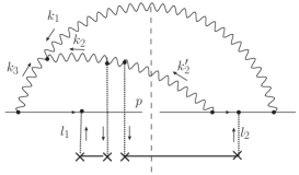
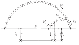
$A$	$B$

Figure 25: $p_{\perp}$-broadening graphs in the case in which two quark-gluon vertices are in the initial state and one is in the final state. The transverse momenta are directed according to the arrows, while the “$+$” momenta are oriented to the right. We do not show the graph $A_{3}^{\prime}$ which is similar to $A$ but with gluon 3 exchanged instantaneously, and $B_{1}^{\prime}$, similar to $B$ but with gluon 1 exchanged instantaneously. Momentum conservation implies that $\vec{k}_{2}^{\prime}=\vec{k}_{2}+\vec{l}_{1}+\vec{l}_{2}$.

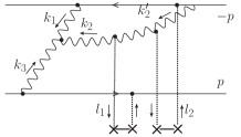
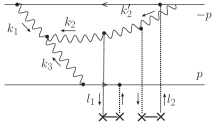
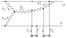
$\alpha$	$\beta$	$\gamma$

Figure 26: Dipole graphs corresponding to the $p_{\perp}$-broadening graphs in Fig. 25. To this list one should add the graphs in which gluons $1$ or $3$ are exchanged instantaneously, and distinguish two relative orderings of the leftmost $qg$ and $\bar{q}g$ vertices in $\gamma$, which we should draw as two different graphs $\gamma^{(1)}$ and $\gamma^{(2)}$.

The calculation of the different contributions using the previously edicted rules (Eq. (18) for the energy denominators, Eqs. (20) and (21) for the eikonal vertices, Eq. 23 for additional factors associated to all vertices, and Tab. 1 for the 3-gluon vertex dressed with the polarization tensors) is straightforward.

We define the energy of the gluons as

$$E_{1}=\frac{\vec{k}_{1}^{2}}{2k_{1+}},\ E_{2}=\frac{\vec{k}_{2}^{2}}{2k_{2+}},\ E^{\prime}_{2}=\frac{\vec{k}_{2}^{\prime 2}}{2k_{2+}}=\frac{(\vec{k}_{2}+\vec{l}_{1}+\vec{l}_{2})^{2}}{2k_{2+}},\ E_{3}=\frac{\vec{k}_{3}^{2}}{2k_{3+}}.$$ (72)

The calculations corresponding to the $A,\alpha$ and $B,\beta$ graphs (without including the lower part of the graphs representing the coupling to the target) are summarized in Tab. 2 and 3. We distinguish the four different polarization configurations (as in Tab. 1) for each graph. The two columns single out the energy denominators (which are not polarization dependent) and the 3-gluon vertex and polarization factors read off Tab. 1 with the relevant kinematics. In addition, there is an overall factor, which is identical for all graphs: After averaging over the color and helicity of the initial quarks, it reads

$$\frac{8\pi^{4}\alpha_{s}^{4}N_{c}^{3}C_{F}}{(k_{1+}k_{2+}k_{3+})^{2}}.$$ (73)

The $2/(k_{1+}k_{2+}k_{3+})$ factor in Tab. 1 has been incorporated in Eq. (73).

In order to compute the contribution of these graphs to $p_{\perp}$-broadening, we need to convolute the content of Tab. 2 and 3 multiplied by Eq. (73) with some weight which encodes the model for the interaction with the target and which can be computed from the rules listed in Sec. 3:

$$\left.\frac{dN}{d^{2}p}\right|_{\text{ \begin{minipage}{85.35826pt} \tiny contribution of a\\ \tiny particular graph \end{minipage}}}=-\int\frac{d^{2}\vec{l}_{1}}{\vec{l}_{1}^{2}}\frac{d^{2}\vec{l}_{2}}{\vec{l}_{2}^{2}}\left[\frac{xg(x,\vec{l}_{1}^{2})}{N_{c}^{2}-1}\rho L\right]\left[\frac{xg(x,\vec{l}_{2}^{2})}{N_{c}^{2}-1}\rho L\right]\\ \times\int_{0}^{+\infty}dk_{1+}dk_{2+}dk_{3+}\delta(\text{``$+$'' momentum})\times\left[\text{overall factor}\right]\\ \times\int\frac{d^{2}\vec{k}_{1}}{(2\pi)^{2}}\frac{d^{2}\vec{k}_{2}}{(2\pi)^{2}}\frac{d^{2}\vec{k}_{3}}{(2\pi)^{2}}\delta^{2}(\vec{k}_{1}+\vec{k}_{2}+\vec{k}_{3})\delta^{2}(\text{global ``$\perp$'' momentum})\\ \times\left[\text{right column of the corresponding table}\right]$$ (74)

where, for example in the case of graph $A$, the graph-dependent momentum conservation factors read

$$\begin{split}\delta(\text{``$+$'' momentum})&\equiv\delta(k_{1+}+k_{2+}-k_{3+})\\ \delta^{2}(\text{global ``$\perp$'' momentum})&\equiv\delta^{2}(\vec{k}_{2}+\vec{p})\\ \left[\text{overall factor}\right]&=\text{Eq.~{}(\ref{eq:overallfactor})}\end{split}$$ (75)

and the “corresponding table” is Tab. 2.

	Energy denom.	3-gluon vertex$\times$pola.
$A_{1}$	$-\frac{1}{E_{1}E^{\prime}_{2}E_{3}(E_{1}+E_{2})}$	$(\vec{k}_{2}^{\prime}\cdot\vec{k}_{3})E_{1}(2k_{3}-k_{1})_{+}$
$A_{2}$		$(\vec{k}_{1}\cdot\vec{k}_{3})(\vec{k}_{2}\cdot\vec{k}_{2}^{\prime})\left[-(k_{1}+k_{3})_{+}/(2(k_{3}-k_{1})_{+})\right]$
$A_{3}^{*}$		$0$
$A_{\perp}$		$\frac{1}{2}\left[(\vec{k}_{2}\cdot\vec{k}_{3})(\vec{k}_{1}\cdot\vec{l})-(\vec{k}_{1}\cdot\vec{k}_{2})(\vec{k}_{3}\cdot\vec{l})\right]$
$\alpha_{1}^{*}$	$\frac{1}{E_{2}E^{\prime}_{2}E_{3}(E_{1}+E_{2})}$	$(\vec{k}_{2}^{\prime}\cdot\vec{k}_{3})(-E_{2})(2k_{3}-k_{1})_{+}$
$\alpha_{2}$		$(\vec{k}_{1}\cdot\vec{k}_{3})(\vec{k}_{2}\cdot\vec{k}_{2}^{\prime})\left[-(k_{1}+k_{3})_{+}/(2(k_{3}-k_{1})_{+})\right]$
$\alpha_{3}^{*}$		$0$
$\alpha_{\perp}$		$\frac{1}{2}\left[(\vec{k}_{2}\cdot\vec{k}_{3})(\vec{k}_{1}\cdot\vec{l})-(\vec{k}_{1}\cdot\vec{k}_{2})(\vec{k}_{3}\cdot\vec{l})\right]$

Table 2: Expressions for the graphs $A$ and $\alpha$ in Fig. 25 and 26. $k^{\prime}_{2}=k_{2}+l$ (where $l=l_{1}+l_{2}$) and according to momentum conservation, $k_{2+}=k_{3+}-k_{1+}$. The “*” superscript on the graph labels means that an instantaneous exchange graph has been added. The factor $2/(k_{1+}k_{2+}k_{3+})$ present in Tab. 1 was left out and integrated to the overall factor (73). The contribution of $A$ to the $p_{\perp}$-broadening amplitude is obtained from the convolution given in Eq. (74).

	Energy denom.	3-gluon vertex$\times$pola.
$B_{1}^{*}$	$\frac{1}{E_{1}E^{\prime}_{2}E_{3}(E_{2}+E_{3})}$	$0$
$B_{2}$		$(k_{1}\cdot k_{3})(k_{2}\cdot k_{2}^{\prime})\left[-(k_{1}+k_{3})_{+}/(2(k_{1}-k_{3})_{+})\right]$
$B_{3}$		$(k_{1}\cdot k_{2}^{\prime})E_{3}(2k_{1}-k_{3})_{+}$
$B_{\perp}$		$-\frac{1}{2}\left[(\vec{k}_{2}\cdot\vec{k}_{3})(\vec{k}_{1}\cdot\vec{l})+(\vec{k}_{1}\cdot\vec{k}_{2})(\vec{k}_{3}\cdot\vec{l})\right]$
$\beta_{1}^{*}$	$\frac{1}{E_{1}E_{2}E_{2}^{\prime}(E_{2}+E_{3})}$	$0$
$\beta_{2}$		$(k_{1}\cdot k_{3})(k_{2}\cdot k_{2}^{\prime})\left[(k_{1}+k_{3})_{+}/(2(k_{1}-k_{3})_{+})\right]$
$\beta_{3}^{*}$		$(k_{1}\cdot k_{2}^{\prime})E_{2}(2k_{1}-k_{3})_{+}$
$\beta_{\perp}$		$\frac{1}{2}\left[(\vec{k}_{2}\cdot\vec{k}_{3})(\vec{k}_{1}\cdot\vec{l})-(\vec{k}_{1}\cdot\vec{k}_{2})(\vec{k}_{3}\cdot\vec{l})\right]$

Table 3: The same as Tab. 2 but for graphs $B$ and $\beta$ in Fig 25 and 26, for which momentum conservation reads $k_{2+}=k_{1+}-k_{3+}$.

From the conservation of 3-momentum and from the positivity of the “+” components, we note that the $A$ and $\alpha$ graphs have the same integration range of the “$+$” components of the momenta, namely $0<k_{1+}<k_{3+}$, while in the case of $B$ and $\beta$, $k_{1+}>k_{3+}$. As for the $\gamma$ graph, $k_{1+}$ and $k_{3+}$ must be both integrated from 0 to $+\infty$. We may subtract the dipole graphs from the production graphs whenever the kinematics are identical. We find that only the “2” and “$\perp$” components are nonzero in the differences $A-\alpha$ and $B-\beta$. They are listed in Tab. 4 together with the nonzero components of $\gamma$. We have specified the integration range and singled out the factors which depend on the “$\perp$” and “$+$” components of the momenta. Other factors are common to all graphs (see the caption of Tab. 4). As for $\gamma$, we were careful to distinguish two possible orderings of the $qg$ and $\bar{q}g$ vertices $\gamma^{(1)}$ and $\gamma^{(2)}$ before adding up their contributions, see the caption of Fig. 26.

	Integration range	Momentum-dependent factors
		“$\perp$”	“+”
$A_{2}-\alpha_{2}$	$0<k_{1+}<k_{3+}$	$\frac{(\vec{k}_{1}\cdot\vec{k}_{3})(\vec{k}_{2}\cdot\vec{k}_{2}^{\prime})}{\vec{k}_{1}^{2}\vec{k}_{2}^{2}\vec{k}_{2}^{\prime 2}\vec{k}_{3}^{2}}$	$\frac{k_{1+}+k_{3+}}{k_{1+}(k_{3+}-k_{1+})k_{3+}}$
$A_{\perp}-\alpha_{\perp}$		$\frac{-(\vec{k}_{2}\cdot\vec{k}_{3})(\vec{k}_{1}\cdot\vec{l})+(\vec{k}_{1}\cdot\vec{k}_{2})(\vec{k}_{3}\cdot\vec{l})}{\vec{k}_{1}^{2}\vec{k}_{2}^{2}\vec{k}_{2}^{\prime 2}\vec{k}_{3}^{2}}$	$\frac{1}{k_{1+}k_{3+}}$
$B_{2}-\beta_{2}$	$k_{1+}>k_{3+}$	$\frac{(\vec{k}_{1}\cdot\vec{k}_{3})(\vec{k}_{2}\cdot\vec{k}_{2}^{\prime})}{\vec{k}_{1}^{2}\vec{k}_{2}^{2}\vec{k}_{2}^{\prime 2}\vec{k}_{3}^{2}}$	$\frac{k_{1+}+k_{3+}}{k_{1+}(k_{3+}-k_{1+})k_{3+}}$
$B_{\perp}-\beta_{\perp}$		$\frac{-(\vec{k}_{2}\cdot\vec{k}_{3})(\vec{k}_{1}\cdot\vec{l})+(\vec{k}_{1}\cdot\vec{k}_{2})(\vec{k}_{3}\cdot\vec{l})}{\vec{k}_{1}^{2}\vec{k}_{2}^{2}\vec{k}_{2}^{\prime 2}\vec{k}_{3}^{2}}$	$\frac{1}{k_{1+}k_{3+}}$
$\gamma_{2}$	$0<k_{1+}<+\infty$	$\frac{(\vec{k}_{1}\cdot\vec{k}_{3})(\vec{k}_{2}\cdot\vec{k}_{2}^{\prime})}{\vec{k}_{1}^{2}\vec{k}_{2}^{2}\vec{k}_{2}^{\prime 2}\vec{k}_{3}^{2}}$	$\frac{k_{3+}-k_{1+}}{k_{1+}(k_{1+}+k_{3+})k_{3+}}$
$\gamma_{\perp}$		$\frac{-(\vec{k}_{2}\cdot\vec{k}_{3})(\vec{k}_{1}\cdot\vec{l})+(\vec{k}_{1}\cdot\vec{k}_{2})(\vec{k}_{3}\cdot\vec{l})}{\vec{k}_{1}^{2}\vec{k}_{2}^{2}\vec{k}_{2}^{\prime 2}\vec{k}_{3}^{2}}$	$\frac{1}{k_{1+}k_{3+}}$

Table 4: Differences between the contributions of graphs $A$,$\alpha$ and $B$, $\beta$ respectively, and nonzero contributions of graph $\gamma$. We only keep the momentum-dependent factors, which we split between a factor depending only on the transverse components, and a factor depending only on the longitudinal ones. (The overall constant, which gathers the coupling and color factors, reads $64\pi^{4}\alpha_{s}^{4}N_{c}^{3}C_{F}$).

We are now in position to prove the equivalence between the production and the dipole processes. We need to compare the results of the integration of the expressions for the different graphs over the $k_{1+}$ variable. We see in Tab. 4 that $A-\alpha$ and $B-\beta$ have exactly the same expressions: The difference is in the integration ranges in $k_{1+}$, which turn out to be complementary on the positive real axis $[0,+\infty[$.

Let us show in detail that the analytical continuation of $\gamma_{2}$ to the negative $k_{1+}$ region has exactly the same expression as $A_{2}-\alpha_{2}$ and $B_{2}-\beta_{2}$, once the change of variable $k_{1+}\rightarrow-k_{1+}$ is done in order to go back to positive $+$ factors.

Figure 27: Complex plane of the $x$-variable in the integrand of Eq. (76).

To this aim, it is enough to focus on the “+” components in Tab. 4 (see the rightmost column) since the labeling conventions have been chosen such that the other factors remain identical for all graphs. We define $x\equiv k_{1+}/k_{3+}$ in order to simplify the equations and write the integral associated to $\gamma_{2}$ as

$$\gamma_{2}\rightarrow I_{+}=\int_{\lambda}^{\Lambda}dx\frac{1-x}{x(1+x)}.$$ (76)

We go to the complex plane of the $x$-variable and sum the integrand over the double contour shown in Fig. 27. The integrals over the semi-circles $I_{\Lambda}$, $I_{\lambda}$, $I_{\varepsilon}$ and their symmetrics give a finite contribution, but their sum vanishes. From the Cauchy theorem, the remaining terms are then related by the equation

$$2(I_{+}+I_{<}+I_{>})=0.$$ (77)

The first term $I_{+}$ is proportional to $\gamma_{2}$. The two other terms read

$$\begin{split}I_{<}&=\int_{-1+\varepsilon}^{-\lambda}dx\frac{1-x}{x(1+x)}=-\int_{\lambda}^{1-\varepsilon}dx\frac{1+x}{x(1-x)}\rightarrow-(A_{2}-\alpha_{2})\\ I_{>}&=\int_{-\Lambda}^{-1-\varepsilon}dx\frac{1-x}{x(1+x)}=-\int_{1+\varepsilon}^{\Lambda}dx\frac{1+x}{x(1-x)}\rightarrow-(B_{2}-\beta_{2})\end{split}$$ (78)

After the limit $\varepsilon,\lambda\rightarrow 0$ and $\Lambda\rightarrow+\infty$ is taken, Eq. (77) shows the equivalence between the $p_{\perp}$-broadening diagrams and the dipole diagrams. The same argument applies to the “$\perp$” component and leads to the same conclusion.

Note using the double contour in Fig. 27 is equivalent to taking a principal-part prescription for the pole at $x=-1$. Originally, this pole was shifted off the real axis by the regularization chosen for the energy denominators. But since the imaginary terms anyway cancel after one has included all relevant graphs, these two choices are equivalent.

Of course, in the present case, the integrals $I_{+}$, $I_{<}$ and $I_{>}$ are simple enough that we can also afford to check directly the identity

$$\int_{0}^{k_{3+}-\varepsilon}dk_{1+}(A_{2,\perp}-\alpha_{2,\perp})+\int_{k_{3+}+\varepsilon}^{+\infty}dk_{1+}(B_{2,\perp}-\beta_{2,\perp})=\int_{0}^{+\infty}dk_{1+}\gamma_{2,\perp},$$ (79)

which holds once appropriate cutoffs have been introduced to regularize the infrared and ultraviolet divergences at $k_{1+}\rightarrow 0$ and $k_{1+}\rightarrow+\infty$ respectively. But the analytical continuation argument presented above appears more general.

Having performed these detailed checks in this simple case, we will be able to compare the graphs in all other cases by going through the following steps:

1. We write the expression for all graphs for all possible polarizations of the gluons, with conventions for the momenta that are such that the same transverse structure is kept for all graphs (This step is summarized in Tab. 2 and 3 in the case just discussed).

2. We choose 2 variables among the 3 “+” components $k_{1+}$, $k_{2+}$, $k_{3+}$ and use momentum conservation in order to express one of them ($k_{2+}$ here) in terms of the other two. We fix one of the remaining variables ($k_{3+}$ here). We group all graphs according to the range of integration of the leftover variable ($k_{1+}$). In each such group, we add up the expressions for the $p_{\perp}$-broadening graphs and subtract the ones for the dipole graphs (Tab. 4).

3. In the class of graphs for which the range of integration is unrestricted (graph $\gamma$ here, see Tab. 4), we invert the sign of the variable on which we integrate ($k_{1+}$ here), and add an overall “$-$” sign to take into account the change of sign in the integration element.

4. The equivalence between $p_{\perp}$-broadening and dipole amplitudes is true if the expressions obtained after this transformation are the same as the expressions found for all other classes of graphs (Eq. (79) in our example).

This procedure is a practical formulation of the analytical continuation method detailed above, which enables one to check at first sight the equivalence.

4.2.2 Initial state/final state

We now turn to the case in which one quark-gluon vertex in the amplitude is in the initial state, while the two other quark-gluon couplings on the right of the cut are in the final state.

In the simplest case, the 3-gluon vertex is also in the initial state. This is shown in Fig. 28.

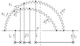
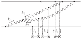
Figure 28: $p_{\perp}$-broadening graph for the configuration in which one quark-gluon coupling and the 3-gluon vertex are in the initial state, while the remaining two $qg$ vertices are in the final state (left) and the equivalent dipole graph (right).

This case is actually straightforward. On one hand, the energy denominators, for $p_{\perp}$-broadening as well as for dipoles, read

$$D=\frac{1}{E^{\prime\prime}_{2}E_{3}(E_{1}+E_{2})(E^{\prime\prime}_{1}+E^{\prime\prime}_{2})}.$$ (80)

On the other hand, all other terms are identical for both graphs.

The graphs in which the 3-gluon vertex is in the final state are shown in Fig. 29 (and Fig. 30 for the corresponding dipole graphs).

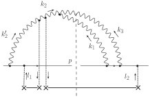
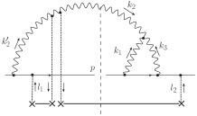
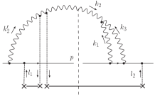
$A$	$B$	$C$

Figure 29: $p_{\perp}$-broadening graphs for the configuration in which all interactions but one quark-gluon coupling occur in the final state (The instantaneous-exchange graphs are not shown).

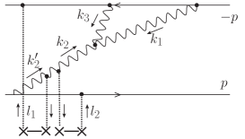
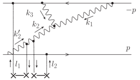
$\alpha$	$\beta$

Figure 30: Dipole graphs corresponding to the $p_{\perp}$-broadening graphs of Fig. 29 (The instantaneous-exchange graphs are not shown).

We may group the graphs $A$, $C$ and $\alpha$ in Fig. 29 and 30 since they share the same kinematics, while we treat separately the graphs $B$ and $\beta$. We do not present the evaluation of all diagrams separately for this case (step 1 in the procedure outlined above) since their expression is very similar to the previous case. We find that the expressions for $A+C-\alpha$ and for $B$ are identical once we express everything in terms of the variables $k_{2+}$ and $k_{3+}$.

The overall factor is again given by Eq. (73). The results for the nonzero components of $A+C-\alpha$, $B$ and $\beta$ are shown in Tab. 5.

	Integration range	Momentum-dependent factors
		pure “$\perp$”	“+” and “$\perp$”
$A_{2}+C_{2}-\alpha_{2}$, $B_{2}$	$k_{3+}<k_{2+}<+\infty$, $0<k_{2+}<k_{3+}$	$\frac{(\vec{k}_{1}\cdot\vec{k}_{3})(\vec{k}_{2}\cdot\vec{k}_{2}^{\prime})}{\vec{k}_{1}^{2}\vec{k}_{2}^{2}\vec{k}_{2}^{\prime 2}}$	$\frac{1}{\vec{k}_{2}^{2}/k_{2+}-\vec{k}_{3}^{2}/k_{3+}}\frac{k_{2+}-2k_{3+}}{(k_{2+}-k_{3+})k_{2+}k_{3+}^{2}}$
$A_{3}+C_{3}^{*}-\alpha_{3}^{*}$, $B_{3}$		$\frac{(\vec{k}_{1}\cdot\vec{k}_{2}^{\prime})}{\vec{k}_{1}^{2}\vec{k}_{2}^{\prime 2}}$	$\frac{1}{\vec{k}_{2}^{2}/k_{2+}-\vec{k}_{3}^{2}/k_{3+}}\frac{2k_{2+}-k_{3+}}{(k_{2+}-k_{3+})k_{2+}k_{3+}^{2}}$
$A_{\perp}+C_{\perp}-\alpha_{\perp}$, $B_{\perp}$		$\frac{(\vec{k}_{2}\cdot\vec{k}_{3})(\vec{k}_{1}\cdot\vec{l})-(\vec{k}_{1}\cdot\vec{k}_{2})(\vec{k}_{3}\cdot\vec{l})}{k_{1}^{2}k_{2}^{2}k_{2}^{\prime 2}}$	$\frac{1}{\vec{k}_{2}^{2}/k_{2+}-\vec{k}_{3}^{2}/k_{3+}}\frac{1}{(k_{2}-k_{3})_{+}k_{3+}^{2}}$
$\beta_{2}$	$0<k_{2+}<+\infty$	$\frac{(\vec{k}_{1}\cdot\vec{k}_{3})(\vec{k}_{2}\cdot\vec{k}_{2}^{\prime})}{\vec{k}_{1}^{2}\vec{k}_{2}^{2}\vec{k}_{2}^{\prime 2}}$	$-\frac{1}{\vec{k}_{2}^{2}/k_{2+}+\vec{k}_{3}^{2}/k_{3+}}\frac{k_{2+}+2k_{3+}}{(k_{2+}+k_{3+})k_{2+}k_{3+}^{2}}$
$\beta_{3}^{*}$		$\frac{(\vec{k}_{1}\cdot\vec{k}_{2}^{\prime})}{\vec{k}_{1}^{2}\vec{k}_{2}^{\prime 2}}$	$-\frac{1}{\vec{k}_{2}^{2}/k_{2+}+\vec{k}_{3}^{2}/k_{3+}}\frac{2k_{2+}+k_{3+}}{(k_{2+}+k_{3+})k_{2+}k_{3+}^{2}}$
$\beta_{\perp}$		$\frac{(\vec{k}_{2}\cdot\vec{k}_{3})(\vec{k}_{1}\cdot\vec{l})-(\vec{k}_{1}\cdot\vec{k}_{2})(\vec{k}_{3}\cdot\vec{l})}{k_{1}^{2}k_{2}^{2}k_{2}^{\prime 2}}$	$-\frac{1}{\vec{k}_{2}^{2}/k_{2+}+\vec{k}_{3}^{2}/k_{3+}}\frac{1}{(k_{2}+k_{3})_{+}k_{3+}^{2}}$

Table 5: Sums and differences of the graphs of Fig. 29 and 30 grouped according to kinematics. The overall constant is $64\pi^{4}\alpha_{s}^{4}N_{c}^{3}C_{F}$.

It is clear that the analytical continuation of the components of the graph $\beta$ in the variable $k_{2+}$ is equal to $A+C-\alpha$ for $k_{2+}>k_{3+}$ and to $B$ for $k_{2+}<k_{3+}$ as far as the real part is concerned. The imaginary parts cancel with the complex conjugate graphs that also have to be taken into account.

4.2.3 Initial state/initial state

We turn to the graphs in which all vertices are in the initial state. First, there is the trivial case of the $p_{\perp}$-broadening graphs in Fig. 31 which cancel in exactly the same way e.g. as the graphs of Fig. 12 cancelled. There is no kinematically-allowed equivalent dipole graph.

We turn to the more interesting graphs in Fig. 32. All interactions between the nucleus and one of the gluons cancel, hence the exchanged gluons necessarily hook to the quark line. The corresponding dipole graphs are virtual (Fig. 33).

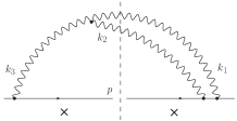
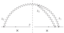
Figure 31: Set of the $p_{\perp}$-broadening graphs for which all interactions occur in the initial state but which cancel. We have not drawn explicitly the gluons exchanged with the target.

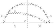
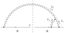
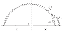
$A$	$B$	$C$

Figure 32: The same as Fig. 31 but for the non-cancelling graphs. The gluons exchanged with the target (not drawn) all couple to the quark line, and thus are not relevant to the discussion of the equivalence.

The evaluation of the $p_{\perp}$-broadening graphs of Fig. 32 is straightforward. The results are presented in Tab. 6.

	Integration range	Energy denom.	3-gluon$\times$pola.
$A_{1}$	$0<k_{1+}<k_{3+}$	$\frac{1}{E_{1}E_{3}(E_{1}+E_{2})^{2}}$	$(\vec{k}_{2}\cdot\vec{k}_{3})E_{1}(2k_{3}-k_{1})_{+}$
$A_{2}$			$(\vec{k}_{1}\cdot\vec{k}_{3})(-E_{2})(k_{1}+k_{3})_{+}$
$A_{3}^{*}$			$0$
$B_{1}^{*}$	$k_{1+}>k_{3+}$	$\frac{1}{E_{1}E_{3}^{2}(E_{2}+E_{3})}$	0
$B_{2}^{*}$			$(\vec{k}_{1}\cdot\vec{k}_{3})E_{3}(k_{1}+k_{3})_{+}$
$B_{3}$			$(\vec{k}_{1}\cdot\vec{k}_{2})E_{3}(2k_{1}-k_{3})_{+}$
$C_{1}$	$0<k_{1+}<k_{3+}$	$\frac{1}{E_{1}E_{3}^{2}(E_{1}+E_{2})}$	$(\vec{k}_{2}\cdot\vec{k}_{3})E_{1}(2k_{3}-k_{1})_{+}$
$C_{2}^{*}$			$(\vec{k}_{1}\cdot\vec{k}_{3})E_{1}(k_{1}+k_{3})_{+}$
$C_{3}$			$(\vec{k}_{1}\cdot\vec{k}_{2})E_{3}(k_{3}-2k_{1})_{+}$

Table 6: Expressions of the graphs of Fig. 32. The momentum conservation reads $k_{2+}=k_{3+}-k_{1+}$ for graphs $A$ and $C$, and $k_{2+}=k_{1+}-k_{3+}$ for graph $B$. These expressions must be multiplied by the overall factor (81).

The dipole graphs in Fig. 33 bring in a new difficulty with respect e.g. to the real graphs in Fig. 28,29,30: The energy denominators diverge, thus it is crucial to keep the regulator $\varepsilon$ throughout. The divergencies are not removed by instantaneous exchanges as was the case for other graphs, but they give imaginary contributions which are cancelled when one adds the complex conjugate graphs. The results are shown in Tab. 7.

$\alpha$	$\beta$	$\gamma$	$\delta^{(1)}$ (up) and $\delta^{(2)}$ (down)

Figure 33: Set of the dipole graphs corresponding to the $p_{\perp}$-broadening graphs of Fig. 32. $\delta^{(1)}$ and $\delta^{(2)}$ differ by the ordering of the absorption times of gluons $2$ and $3$. $\gamma$ actually represents 2 graphs, which differ by the order of the leftmost $\bar{q}g$ and $qg$ vertices.

	Integration range	Energy denominators	3-gluon vertex$\times$pola.
$\alpha_{1}^{*}$	$0<k_{1+}<k_{3+}$	$-\frac{1}{4i\varepsilon}\frac{1}{(E_{2}-3i\varepsilon)(E_{3}-i\varepsilon)(E_{1}+E_{2}-2i\varepsilon)}$	$(\vec{k}_{2}\cdot\vec{k}_{3})(2i\varepsilon-E_{2})(2k_{3}-k_{1})_{+}$
$\alpha_{2}$			$(\vec{k}_{1}\cdot\vec{k}_{3})(-E_{2})(k_{1}+k_{3})_{+}$
$\alpha_{3}^{*}$			$(\vec{k}_{1}\cdot\vec{k}_{2})(i\varepsilon)(k_{3}-2k_{1})_{+}$
$\beta_{1}$		$-\frac{1}{4i\varepsilon}\frac{1}{(E_{1}-i\varepsilon)(E_{3}-3i\varepsilon)(E_{1}+E_{2}-2i\varepsilon)}$	$(\vec{k}_{2}\cdot\vec{k}_{3})(-E_{1})(2k_{3}-k_{1})_{+}$
$\beta_{2}^{*}$			$(\vec{k}_{1}\cdot\vec{k}_{3})(2i\varepsilon-E_{1})(k_{1}+k_{3})_{+}$
$\beta_{3}^{*}$			$(\vec{k}_{1}\cdot\vec{k}_{2})(3i\varepsilon)(2k_{1}-k_{3})_{+}$
$\gamma_{1}^{*}$	$0<k_{1+}<+\infty$	$-\frac{1}{4i\varepsilon}\frac{1}{(E_{1}-i\varepsilon)(E_{3}-i\varepsilon)(E_{2}-2i\varepsilon)}$	$(\vec{k}_{2}\cdot\vec{k}_{3})(i\varepsilon)(2k_{3}+k_{1})_{+}$
$\gamma_{2}^{*}$			$(\vec{k}_{1}\cdot\vec{k}_{3})(3i\varepsilon)(k_{3}-k_{1})_{+}$
$\gamma_{3}^{*}$			$(\vec{k}_{1}\cdot\vec{k}_{2})(-i\varepsilon)(2k_{1}+k_{3})_{+}$
$\delta_{1}^{(1)*}$	$k_{3+}<k_{1+}<+\infty$	$-\frac{1}{4i\varepsilon}\frac{1}{(E_{1}-i\varepsilon)(E_{2}+E_{3}-2i\varepsilon)(E_{2}-3i\varepsilon)}$	$(\vec{k}_{2}\cdot\vec{k}_{3})(i\varepsilon)(2k_{3}-k_{1})_{+}$
$\delta_{2}^{(1)}$			$(\vec{k}_{1}\cdot\vec{k}_{3})E_{2}(k_{1}+k_{3})_{+}$
$\delta_{3}^{(1)*}$			$(\vec{k}_{1}\cdot\vec{k}_{2})(E_{2}-2i\varepsilon)(2k_{1}-k_{3})_{+}$
$\delta_{1}^{(2)*}$		$-\frac{1}{4i\varepsilon}\frac{1}{(E_{1}-i\varepsilon)(E_{2}+E_{3}-2i\varepsilon)(E_{3}-3i\varepsilon)}$	$(\vec{k}_{2}\cdot\vec{k}_{3})(i\varepsilon)(2k_{3}-k_{1})_{+}$
$\delta_{2}^{(2)*}$			$(\vec{k}_{1}\cdot\vec{k}_{3})(2i\varepsilon-E_{3})(k_{1}+k_{3})_{+}$
$\delta_{3}^{(2)}$			$(\vec{k}_{1}\cdot\vec{k}_{2})(-E_{3})(2k_{1}-k_{3})_{+}$

Table 7: Expressions of the graphs of Fig. 33. The momentum conservation reads $k_{2+}=k_{3+}-k_{1+}$ for graphs $\alpha$ and $\beta$, $k_{2+}=k_{1+}+k_{3+}$ for graph $\gamma$, and $k_{2+}=k_{1+}-k_{3+}$ for graph $\delta$. These expressions must be multiplied by the overall factor (81). The contribution to $p_{\perp}$-broadening is obtained by convoluting with the weight given in Eq. (74).

The overall factor, including the averaging over the color and helicity of the quark, reads

$$-\frac{32\pi^{4}\alpha_{s}^{4}N_{c}C_{F}^{3}}{(k_{1+}k_{2+}k_{3+})^{2}},$$ (81)

which is identical to (73) in the large-$N_{c}$ limit ($C_{F}\simeq N_{c}/2$) except for the sign.

Again, we may put together the graphs with the same kinematics. This is shown in Tab. 8. We have left out some imaginary terms, namely

$$\begin{split}\text{Im}(A_{1}+C_{1}-\alpha_{1}^{*}-\beta_{1})&\propto\frac{1}{\varepsilon\vec{k}_{3}^{2}(\vec{k}_{1}^{2}(k_{3+}-k_{1+})+\vec{k}_{2}^{2}k_{1+})}\frac{(2k_{3}-k_{1})_{+}}{k_{1+}(k_{3}-k_{1})_{+}k_{3+}}\\ \text{Im}(A_{2}+C_{2}^{*}-\alpha_{2}-\beta_{2}^{*})&\propto\frac{1}{\varepsilon\vec{k}_{3}^{2}(\vec{k}_{1}^{2}(k_{3+}-k_{1+})+\vec{k}_{2}^{2}k_{1+})}\frac{(k_{1}+k_{3})_{+}}{k_{1+}(k_{3}-k_{1})_{+}k_{3+}}\end{split}$$ (82)

which are divergent. The instantaneous-exchange graphs are not enough to remove all divergencies, as they do in other cases. But these terms do not play any rôle in our discussion since we must eventually add all complex conjugate graphs together.

	Integration range	Momentum-dependent factors
		“$\perp$”	“+”
$\text{Re}(A_{1}+C_{1}-\alpha_{1}^{*}-\beta_{1})$, $B_{1}^{*}-\delta_{1}^{*}$	$0<k_{1+}<k_{3+}$, $k_{3+}<k_{1+}<+\infty$	$\frac{\vec{k}_{2}\cdot\vec{k}_{3}}{\vec{k}_{1}^{2}\vec{k}_{2}^{2}\vec{k}_{3}^{2}}$	$\frac{(2k_{3}-k_{1})_{+}}{(k_{1}-k_{3})_{+}k_{1+}k_{3+}}$
$\text{Re}(A_{2}+C_{2}^{*}-\alpha_{2}-\beta_{2}^{*})$, $B_{2}^{*}-\delta_{2}^{*}$		$\frac{\vec{k}_{1}\cdot\vec{k}_{3}}{\vec{k}_{1}^{2}\vec{k}_{2}^{2}\vec{k}_{3}^{3}}$	$\frac{3(k_{1}+k_{3})_{+}}{(k_{1}-k_{3})_{+}k_{1+}k_{3+}}$
$A_{3}^{*}+C_{3}-\alpha_{3}^{*}-\beta_{3}$, $B_{3}-\delta_{3}^{*}$		$\frac{\vec{k}_{1}\cdot\vec{k}_{2}}{\vec{k}_{1}^{2}\vec{k}_{2}^{2}\vec{k}_{3}^{2}}$	$\frac{(2k_{1}-k_{3})_{+}}{(k_{1}-k_{3})_{+}k_{1+}k_{3+}}$
$\gamma_{1}^{*}$	$0<k_{1+}<+\infty$	$\frac{\vec{k}_{2}\cdot\vec{k}_{3}}{\vec{k}_{1}^{2}\vec{k}_{2}^{2}\vec{k}_{3}^{2}}$	$-\frac{(k_{1}+2k_{3})_{+}}{(k_{1}+k_{3})_{+}k_{1+}k_{3+}}$
$\gamma_{2}^{*}$		$\frac{\vec{k}_{1}\cdot\vec{k}_{3}}{\vec{k}_{1}^{2}\vec{k}_{2}^{2}\vec{k}_{3}^{2}}$	$\phantom{-}\frac{3(k_{1}-k_{3})_{+}}{(k_{1}+k_{3})_{+}k_{1+}k_{3+}}$
$\gamma_{3}^{*}$		$\frac{\vec{k}_{1}\cdot\vec{k}_{2}}{\vec{k}_{1}^{2}\vec{k}_{2}^{2}\vec{k}_{3}^{2}}$	$\phantom{-}\frac{(2k_{1}+k_{3})_{+}}{(k_{3}+k_{1})_{+}k_{1+}k_{3+}}$

Table 8: Sums and differences of the graphs of Fig. 32 and 33 grouped according to kinematics. The overall constant to be added reads $-64\pi^{4}\alpha_{s}^{4}N_{c}C_{F}^{3}$.

4.2.4 Final state/final state

We now move on to the case in which all interactions are in the final state (Fig. 34). To make the comparison to dipoles easier, we exchange the labeling of gluons 1 and 2 in such a way that gluon 2 is always the one whose coupling to the quark is closer to the interaction with the target than gluon 1. The weights of the graphs $A,B,C$ are shown in Tab. 9.

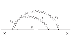
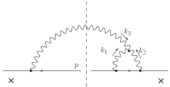
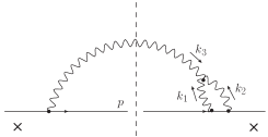
$A$	$B$	$C$

Figure 34: $p_{\perp}$-broadening graphs in which all radiation is in the final state.

	Integration range	Energy denominators	3-gluon vertex$\times$pola.
$A_{1}$	$0<k_{2+}<k_{3+}$	$\frac{1}{E_{1}(E_{1}+E_{2})^{2}(E_{1}+E_{2}-E_{3})}$	$(\vec{k}_{2}\cdot\vec{k}_{3})(-E_{1})(k_{2}+k_{3})_{+}$
$A_{2}$			$(\vec{k}_{1}\cdot\vec{k}_{3})E_{2}(2k_{3}-k_{2})_{+}$
$A_{3}^{*}$			$(\vec{k}_{1}\cdot\vec{k}_{2})(E_{1}+E_{2})(k_{3}-2k_{2})_{+}$
$B_{1}^{*}$	$k_{3+}<k_{2+}<+\infty$	$\frac{1}{E_{1}E_{3}^{2}(E_{2}-E_{3})}$	0
$B_{2}^{*}$			$(\vec{k}_{1}\cdot\vec{k}_{3})E_{3}(k_{2}-2k_{3})_{+}$
$B_{3}$			$(\vec{k}_{1}\cdot\vec{k}_{2})E_{3}(2k_{2}-k_{3})_{+}$
$C_{1}^{*}$	$0<k_{2+}<k_{3+}$	$\frac{1}{E_{3}^{2}(E_{2}-E_{3})(E_{1}+E_{2}-E_{3})}$	$(\vec{k}_{2}\cdot\vec{k}_{3})(E_{2}-E_{3})(k_{2}+k_{3})_{+}$
$C_{2}$			$(\vec{k}_{1}\cdot\vec{k}_{3})E_{2}(2k_{3}-k_{2})_{+}$
$C_{3}$			$(\vec{k}_{1}\cdot\vec{k}_{2})E_{3}(k_{3}-2k_{2})_{+}$

Table 9: Expressions for the graphs of Fig. 34 where all interactions are in the final state. The overall factor is given by Eq. (81).

The corresponding dipole graphs are just the complex conjugates of the graphs in Fig. 33, i.e. the mirror-symmetric graphs. Thus they do not need to be computed again and we may directly group the graphs according to the kinematics. This is shown in Tab. 10. Note that this time, $B$ has the same kinematics as $\gamma$.

	Integration range	Momentum-dependent factors
		“+”, “$\perp$”
$A_{1}+C_{1}^{*}-\alpha_{1}^{*}-\beta_{1}$, $B_{1}^{*}-\gamma_{1}^{*}$	$0<k_{2+}<k_{3+}$, $k_{3+}<k_{2+}<+\infty$	$-\frac{(k_{2}+k_{3})_{+}}{(k_{3}-k_{2})_{+}k_{2+}k_{3+}}$
$A_{2}+C_{2}-\alpha_{2}-\beta_{2}^{*}$, $B_{2}^{*}-\gamma_{2}^{*}$		$\left[1+\frac{4}{(\vec{k}_{2}^{2}k_{3+})/(\vec{k}_{3}^{2}k_{2+})-1}\right]\frac{(2k_{3}-k_{2})_{+}}{(k_{3}-k_{2})_{+}k_{2+}k_{3+}}$
$A_{3}^{*}+C_{3}-\alpha_{3}^{*}-\beta_{3}^{*}$, $B_{3}-\gamma_{3}^{*}$		$\left[-1+\frac{4}{1-(\vec{k}_{3}^{2}k_{2+})/(\vec{k}_{2}^{2}k_{3+})}\right]\frac{(k_{3}-2k_{2})_{+}}{(k_{3}-k_{2})_{+}k_{2+}k_{3+}}$
$\delta_{1}^{*}$	$0<k_{2+}<+\infty$	$\frac{(k_{2}-k_{3})_{+}}{(k_{3}+k_{2})_{+}k_{2+}k_{3+}}$
$\delta_{2}^{*}$		$\left[1-\frac{4}{(\vec{k}_{2}^{2}k_{3+})/(\vec{k}_{3}^{2}k_{2+})+1}\right]\frac{(2k_{3}+k_{2})_{+}}{(k_{3}+k_{2})_{+}k_{2+}k_{3+}}$
$\delta_{3}^{*}$		$\left[-1+\frac{4}{1+(\vec{k}_{3}^{2}k_{2+})/(\vec{k}_{2}^{2}k_{3+})}\right]\frac{(k_{3}+2k_{2})_{+}}{(k_{3}+k_{2})_{+}k_{2+}k_{3+}}$

Table 10: Sums and differences of the graphs of Fig. 34 and 33 grouped according to kinematics. The transverse momentum-dependent factors are not shown since they are the same as in Tab. 8 (third column). Only the real part of the graphs are shown. The global constant reads again $-64\pi^{4}\alpha_{s}^{4}N_{c}C_{F}^{3}$.

We also see that although the calculation is similar to the case in which all interaction vertices are at early times, the resuls shown in Tab. 10 are quite more complicated than the ones shown in Tab. 8.

But again, it is clear that the analytical continuation of $\delta$ in the $k_{2+}$ variable is equal to $A+C-\alpha-\beta$ and $B-\gamma$ in their respective integration domains, which proves the equivalence between $p_{\perp}$-broadening and dipole amplitudes also in this configuration.

4.3 Four quark-gluon vertices

We address the case in which there are four quark-gluon vertices in the evolution of the wave function, linked by two bare gluons.

Writing the expressions for these graphs is quite straightforward since we treat all vertices eikonally: The two gluons both carry the $(--)$ polarization, and so the overall factors need not be discussed since they are identical for all graphs of similar topologies (except for the minus signs already discussed in several occasions which stem from the couplings of the gluons to the antiquark in the dipole case). Only the energy denominators are relevant for the comparison.

We name the $p_{\perp}$-broadening graphs according to the chronology of the four $qg$ vertices, distinguishing the graphs in which the loops are nested by a “hat”.

A relevant way to classify the graphs is to distinguish between interference graphs between the initial and final states, and graphs in which the gluons are emitted and reabsorbed either in the initial and final state.

4.3.1 Interference graphs between initial and final state

Two $qg$ vertices in the initial state, two in the final state.

${\widehat{\text{II}\overline{\text{FF}}}}$ (left),${\widehat{\text{IIF}\overline{\text{F}}}}$ (right)

Figure 35: Four quark-gluon vertex graph. This is an interference graph between the initial and final state, with 2 couplings in each. There are two possible nontrivial cuts.

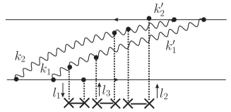
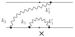
$\gamma_{1}$	$\gamma_{2}$

Figure 36: Dipole graphs corresponding respectively to the left and right cuts of the $p_{\perp}$-broadening graph in Fig. 35. As for $\gamma_{2}$, there are two possible orderings between the $\bar{q}g$ and $qg$ vertices in the complex-conjugate dipole amplitude.

We first address the graph in Fig. 35 which has two $qg$ vertices in the initial state, and two at late times. There may be either two gluons (leftmost cut) or one gluon (rightmost cut) in the final state. These graphs are topologically related to the dipole graphs $\gamma_{1}$ and $\gamma_{2}$ respectively, shown in Fig. 36, which both have 3 dipoles at the time of the interaction. We are going to show that the expressions for these graphs are indeed identical.

The energy denominators read

$$\begin{split}D_{\widehat{\text{II}\overline{\text{FF}}}}&=\frac{1}{E^{\prime}_{1}E_{2}(E_{1}+E_{2})(E_{1}^{\prime}+E_{2}^{\prime})}=D_{\gamma_{1}}\\ D_{\widehat{\text{IIF}\overline{\text{F}}}}&=-\frac{1}{E^{\prime}_{1}E^{\prime}_{2}E_{2}(E_{1}+E_{2})}=-\sum D_{\gamma_{2}}\end{split}$$ (83)

The $\sum$ sign recalls that $\gamma_{2}$ in Fig. 36 actually represents two lightcone perturbation theory graphs, differing by the ordering of some vertices. The definition of the energies may be inferred by applying momentum conservation to the graphs in Fig. 35 and 36. The only important point is that the routing of the momenta be the same in the $p_{\perp}$-broadening and dipole cases. The “$-$” sign in the second line of Eq. (83) corresponds to the change of one gluon coupling from a quark to an antiquark (while for the first graph, two such $qg$ couplings become $\bar{q}g$ couplings, in such a way that the associated minus signs cancel each other).

Note that the first equality in Eq. (83) is straightforward: It is a simple graph-to-graph correspondence. We shall not address exhaustively all such trivial cases in what follows.

We now consider the graph shown in Fig. 37 (as well as its dipole partner in Fig. 38). We need to write the full expressions of the contribution of the graphs to the amplitudes since as we will discover, analytical continuation is needed. This is also the opportunity to show how the complete calculation goes in the four $qg$-vertex case.

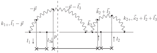
${\text{I}\overline{\text{IFF}}}$

Figure 37: A $p_{\perp}$-broadening diagram whose identification with the corresponding dipole graph requires analytical continuation. A similar diagram (not drawn) would have the cut passing on the rightmost gluon, but the calculation would be the same.

The energy denominators read

$$D_{{\text{I}\overline{\text{IFF}}}}=\frac{1}{(E_{1}-i\varepsilon)(E^{\prime}_{1}-i\varepsilon)(E^{\prime}_{1}-E_{2}-2i\varepsilon)(E^{\prime}_{2}+i\varepsilon)}$$ (84)

where

$$E_{1}=\frac{(\vec{l}_{1}-\vec{p})^{2}}{2k_{1+}}\ ,\ E^{\prime}_{1}=\frac{(\vec{p}+\vec{l}_{3})^{2}}{2k_{1+}}\ ,\ E_{2}=\frac{\vec{k}_{2}^{2}}{2k_{2+}}\ ,\ E^{\prime}_{2}=\frac{(\vec{k}_{2}+\vec{l}_{2}+\vec{l}_{3})^{2}}{2k_{2+}}$$ (85)

(see Fig. 37). The polarization factors for the gluons read

$$\left[d_{-\perp}(l_{1}-p)d_{\perp\perp}(-p)d_{\perp-}(-p-l_{3})\right]\left[d_{-\perp}(k_{2})d_{\perp\perp}(k_{2}+l_{3})d_{\perp-}(k_{2}+l_{2}+l_{3})\right]\\ =\left[\frac{(\vec{p}-\vec{l}_{1})\cdot(\vec{p}+\vec{l}_{3})}{k_{1+}^{2}}\right]\left[\frac{\vec{k}_{2}\cdot(\vec{k}_{2}+\vec{l}_{2}+\vec{l}_{3})}{k_{2+}^{2}}\right].$$ (86)

The vertices are all eikonal. After having performed the sum over the colors of the gluons and averaged over the color of the quark, the associated factor reads

$$-\frac{16\pi^{5}\alpha_{s}^{5}}{k_{1+}k_{2+}}N_{c}^{4}C_{F}.$$ (87)

The factors (84),(86) and (87) must be convoluted with the gluon densities as

$$-\frac{1}{3}\int\frac{dk_{1+}}{(2\pi)^{3}}\frac{dk_{2+}d^{2}\vec{k}_{2}}{(2\pi)^{3}}\frac{d^{2}\vec{l}_{1}}{\vec{l}_{1}^{2}}\frac{d^{2}\vec{l}_{2}}{\vec{l}_{2}^{2}}\frac{d^{2}\vec{l}_{3}}{\vec{l}_{3}^{2}}\frac{xg(x,\vec{l}_{1}^{2})}{N_{c}^{2}-1}\frac{xg(x,\vec{l}_{2}^{2})}{N_{c}^{2}-1}\frac{xg(x,\vec{l}_{3}^{2})}{N_{c}^{2}-1}(\rho L)^{3}$$ (88)

(Momentum conservation was used to get rid of the integration over $\vec{k}_{1}$). The $\frac{1}{3}$ factor comes from the ordering of the times at which the gluons interact with the nucleus. We may perform the integration over the + component of the loop momentum $k_{2}$ explicitly. The result reads

$$\left.\frac{dN}{d^{2}\vec{p}}\right|_{\mbox{\footnotesize Fig. \ref{q4i(ffi)}}}=\frac{1}{3}\frac{\alpha_{s}^{2}N_{c}^{3}}{(N_{c}^{2}-1)^{2}}\int\frac{d^{2}\vec{l}_{1}}{\vec{l}_{1}^{2}}\frac{d^{2}\vec{l}_{2}}{\vec{l}_{2}^{2}}\frac{d^{2}\vec{l}_{3}}{\vec{l}_{3}^{2}}\\ \times\left[{\alpha_{s}xg(x,\vec{l}_{1}^{2})}\right]\left[{\alpha_{s}xg(x,\vec{l}_{2}^{2})}\right]\left[{\alpha_{s}xg(x,\vec{l}_{3}^{2})}\right](\rho L)^{3}\times(\vec{p}-\vec{l}_{1})\cdot(\vec{p}+\vec{l}_{3})\\ \times\int\frac{dk_{1+}}{k_{1+}^{3}}\frac{1}{(E_{1}-i\varepsilon)(E^{\prime}_{1}-i\varepsilon)}\left[\ln\frac{\lambda}{\zeta k_{1+}}+i\pi\right]\int\frac{d^{2}\vec{k}_{2}}{2\pi}\frac{\vec{k}_{2}\cdot(\vec{k}_{2}+\vec{l}_{2}+\vec{l}_{3})}{\vec{k}_{2}^{2}(\vec{k}_{2}+\vec{l}_{2}+\vec{l}_{3})^{2}}$$ (89)

The remaining integral over $k_{1+}$ may also be performed. Instead, we stress that the content of the square brackets in the last line is the result of the integration

$$I_{+}=\int_{\lambda}^{\Lambda}dk_{2+}\frac{\zeta k_{1+}}{k_{2+}(k_{2+}-\zeta k_{1+}-i\eta)}$$ (90)

where $\zeta=\vec{k}_{2}^{2}/(\vec{p}+\vec{l}_{3})^{2}$, and $\eta=4\varepsilon\zeta k_{1+}^{2}/\vec{k}_{2}^{2}$ is a small positive regulator. The IR and UV cutoffs are eventually sent to the limits $\lambda\rightarrow 0$ and $\Lambda\rightarrow+\infty$.

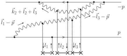
Figure 38: Dipole graph that corresponds to the $p_{\perp}$-broadening graph of Fig. 37. The + components $k_{1+}$ and $k_{2+}$ are always directed to the right. The direction of the transverse components is indicated by the arrows above the gluon lines. There are actually two graphs, which are distinguished by the respective ordering of the $qg$ and $\bar{q}g$ vertices in the amplitude (leftmost vertices). Note that this graph is related to $\gamma_{2}$ in Fig. 36 by a simple symmetry.

We now address the corresponding dipole diagram shown in Fig. 38. We are going to show that its evaluation leads to the same expression as in Eq. (89). We observe that we may label the transverse momenta of the gluons in such a way that only one factor looks different with respect to the previous diagram, namely $I_{+}$. Indeed, the overall difference between the two graphs is in the expression for the energy denominators, which now read (compare to Eq. (84))

$$\frac{1}{(E_{1}-i\varepsilon)(E^{\prime}_{1}+i\varepsilon)(E^{\prime}_{1}+E_{2}+2i\varepsilon)(E^{\prime}_{2}-i\varepsilon)}.$$ (91)

Then $I_{+}$ is replaced by

$$I^{\prime}_{+}=-\int_{\lambda}^{\Lambda}dk_{2+}\frac{\zeta k_{1+}}{k_{2+}(k_{2+}+\zeta k_{1+}+i\eta)},$$ (92)

whose explicit expression reads

$$I^{\prime}_{+}=\ln\frac{\lambda}{\zeta k_{1+}}=I_{+}-i\pi.$$ (93)

Hence the dipole amplitude differs from the $p_{\perp}$-broadening amplitude by an imaginary term, which cancels when one adds the complex conjugate graphs.

We shall now present an alternative way to view the connection between the $p_{\perp}$-broadening diagram and the dipole diagram essentially similar to the analytical continuation presented before. We remind that this method has the advantage that it does not require the explicit evaluation of the integrals, hence it is generalizable to cases in which the latter is not possible.

Figure 39: Integration contour in the $k_{2+}$ plane. The closed contour is divided in 4 sections: $I_{\lambda}$ is the small half circle of radius $\lambda$ oriented clockwise, $I_{+}$ the part $[\lambda,\Lambda]$ of the real axis, $I_{\Lambda}$ the large half circle of radius $\Lambda$ oriented anticlockwise and $I_{-}=[-\Lambda,-\lambda]$. The position of the pole $\zeta k_{1+}+i\eta$ is also shown.

It is based on the observation that the only difference between the two formulations is a change of the direction of the $k_{2+}$ momentum. We are going to interpret this change as an analytical continuation of the integral $I_{+}$. We start with the expression of $I_{+}$ in Eq. (90). The $k_{2+}$ plane is represented in the plot of Fig. 39. The integral in Eq. (90) is represented by the branch along the positive axis of the contour in the figure. The Cauchy theorem on the full contour reads

$$I_{+}+I_{\Lambda}+I_{-}+I_{\lambda}={2i\pi}$$ (94)

where the right-hand side is the contribution of the pole at $k_{2+}=\zeta k_{1+}+i\eta$. $I_{\Lambda}$ is zero when $\Lambda$ goes to infinity since the integral is convergent in the ultraviolet, and it is easy to see that $I_{\lambda}=i\pi$ when $\lambda$ goes to zero. Finally,

$$I_{-}=\int_{-\Lambda}^{-\lambda}\frac{dk_{2+}}{k_{2+}}\frac{\zeta k_{1+}}{k_{2+}-\zeta k_{1+}-i\eta}=\int_{\lambda}^{\Lambda}\frac{dk_{2+}}{k_{2+}}\frac{\zeta k_{1+}}{k_{2+}+\zeta k_{1+}+i\eta}\\ =-I^{\prime}_{+}$$ (95)

Thus, from Eq. (94) and (95), we get

$$I_{+}=i\pi+I^{\prime}_{+}$$ (96)

which is of course the same equation as (93) and thus leads to the same conclusion as before.

Note that here, we chose to stick to the adiabatic regularization while we used the principal part prescription in Sec. 4.2. The difference is in imaginary terms which anyway cancel when all complex conjugate graphs are taken into account.

Three gluons in the initial state, one in the final state.

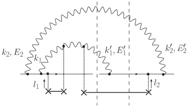
${\widehat{\text{II}\overline{\text{IF}}}}$ (left cut), ${\widehat{\text{IIF}\overline{\text{I}}}}$ (right cut)

Figure 40: $p_{\perp}$-broadening graphs with three $qg$ vertices at early times and one at late times, and two gluons (left cut) or one (right cut) in the final state.

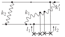
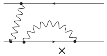
$\beta_{1}$	$\beta_{2}$

Figure 41: Dipole graphs that correspond to the two cuts of the $p_{\perp}$-broadening graph of Fig. 40. For each of these graphs, the graphs corresponding to different orderings of the $\bar{q}g$ vertices with respect to the $qg$ vertex in the amplitude are understood, and this also includes the instantaneous exchange of gluon 2.

Let us address the case in which there is only one $qg$ vertex after the time of the interaction with the nucleus in the $p_{\perp}$-broadening case (which corresponds to 2 real dipoles). The relevant graph (with its two possible cuts) is represented in Fig. 40, and the topologically equivalent dipole graphs are shown in Fig. 41. We find that the energy denominators for these graphs read

$$D_{\widehat{\text{II}\overline{\text{IF}}}}=-D_{\widehat{\text{IIF}\overline{\text{I}}}}=-\frac{1}{E_{1}^{\prime}E_{2}^{2}(E_{1}+E_{2})}=\sum D_{\beta_{1}}=\sum D_{\beta_{2}}.$$ (97)

Again, the $\sum$ signs recall that we have included all relevant graphs, see the caption of Fig. 41. The minus sign in front of $D_{\widehat{\text{IIF}\overline{\text{I}}}}$ eventually gets cancelled when one goes to dipoles by the minus sign of the $\bar{q}g$ vertex in $\beta_{2}$. Thus the correspondence is verified also for these graphs, namely

$${\widehat{\text{II}\overline{\text{IF}}}}\longleftrightarrow\sum\beta_{1}\ ,\ {\widehat{\text{IIF}\overline{\text{I}}}}\longleftrightarrow\sum\beta_{2}\ .$$ (98)

This is almost a graph-to-graph identity, up to the relative position of some vertices in the dipole case.

We move on to the case in which the loops are disconnected. The relevant graphs are shown in Fig. 42 for $p_{\perp}$ broadening, and in Fig. 41 for their dipole equivalent $\beta_{3}$ and $\beta_{4}$. Interestingly enough, there is no graph-by-graph correspondence although the topologies of ${\text{III}\overline{\text{F}}}$ and ${\text{IIF}\overline{\text{I}}}$ seem identical to the topologies of $\beta_{3}$ and $\beta_{4}$ respectively.

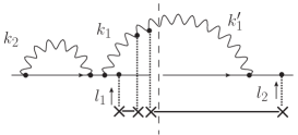
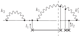
${\text{III}\overline{\text{F}}}$	${\text{IIF}\overline{\text{I}}}$

Figure 42: Graphs for which 3 quark-gluon vertices are in the initial state, one in the final state, and the gluon loops are disjoint.

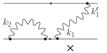
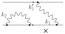
$\beta_{3}$	$\beta_{4}$

Figure 43: Dipole graphs that correspond to the $p_{\perp}$-broadening graphs of Fig. 42. The $\bar{q}g$ vertex in graph $\beta_{4}$ may arrive at any time in $]-\infty,0[$; Only the graph in which it is posterior to the gluon loop is shown.

Indeed, the denominators read

$$\begin{split}D_{\text{III}\overline{\text{F}}}&=\frac{1}{2i\varepsilon(E_{1}-3i\varepsilon)(E^{\prime}_{1}-i\varepsilon)(E_{2}-i\varepsilon)},\\ \text{while}\ \ \ \ D_{\beta_{3}}&=-\frac{1}{2i\varepsilon(E_{1}-3i\varepsilon)(E^{\prime}_{1}+i\varepsilon)(E_{2}-i\varepsilon)}.\end{split}$$ (99)

The difference in the global sign is explained by the $qg\rightarrow\bar{q}g$ change when one goes to dipoles, but there is an extra sign difference in the energy denominator involving $E^{\prime}_{1}$ which hampers the identification of ${\text{III}\overline{\text{F}}}$ and $\beta_{3}$. On the other hand, the remaining diagrams have the following denominators:

$$\begin{split}D_{\text{IIF}\overline{\text{I}}}&=\frac{1}{2i\varepsilon(E_{1}+i\varepsilon)(E^{\prime}_{1}+i\varepsilon)(E_{2}-i\varepsilon)},\\ \sum D_{\beta_{4}}&=-\frac{1}{2i\varepsilon(E_{1}+i\varepsilon)(E^{\prime}_{1}-i\varepsilon)(E_{2}-i\varepsilon)},\end{split}$$ (100)

and thus we see that the sum of all graphs satisfy the identity

$$D_{\text{III}\overline{\text{F}}}+D_{\text{IIF}\overline{\text{I}}}=\frac{1}{i\varepsilon E_{1}E^{\prime}_{1}E_{2}}+\frac{1}{E_{1}^{2}E^{\prime}_{1}E_{2}}+\frac{1}{E_{1}E^{\prime}_{1}E_{2}^{2}}=-(D_{\beta_{3}}+\sum D_{\beta_{4}}).$$ (101)

Hence the correspondence holds between the sum of the $p_{\perp}$-broadening graphs ${\text{III}\overline{\text{F}}}+{\text{IIF}\overline{\text{I}}}$ (left-hand side) and the sum of the dipole graphs $\beta_{3}+\sum{\beta_{4}}$ (right-hand side).

One $qg$ vertex in the initial state, three in the final state.

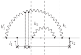
${\widehat{\text{I}\overline{\text{FFF}}}}$,${\widehat{\text{IF}\overline{\text{FF}}}}$,${\widehat{\text{IFF}\overline{\text{F}}}}$	${\widehat{\text{F}\overline{\text{IFF}}}}$,${\widehat{\text{FF}\overline{\text{IF}}}}$,${\widehat{\text{FFF}\overline{\text{I}}}}$	${\text{I}\overline{\text{FFF}}}$,${\text{IFF}\overline{\text{F}}}$	${\text{F}\overline{\text{IFF}}}$,${\text{FFF}\overline{\text{I}}}$

Figure 44: $p_{\perp}$-broadening graphs for the case in which there are 3 $qg$ vertices in the final state.

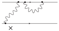
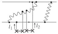
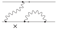
Figure 45: Dipole graphs which are topologically equivalent to ${\widehat{\text{I}\overline{\text{FFF}}}}$, ${\widehat{\text{IF}\overline{\text{FF}}}}$ and ${\widehat{\text{IFF}\overline{\text{F}}}}$ respectively in Fig. 44 (Similar graphs would correspond to ${\widehat{\text{F}\overline{\text{IFF}}}}$, ${\widehat{\text{FF}\overline{\text{IF}}}}$ and ${\widehat{\text{FFF}\overline{\text{I}}}}$).

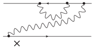
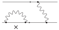
Figure 46: Dipole graphs topologically equivalent to ${\text{I}\overline{\text{FFF}}}$ and ${\text{IFF}\overline{\text{F}}}$ in Fig. 44.

As for the case in which there are 3 $qg$ vertices in the final state (Fig. 44), one finds similar relations with dipole graphs of the type of those represented in Fig. 45 and Fig. 46. We may for example check that

$$D_{\widehat{\text{IF}\overline{\text{FF}}}}=\bar{D}_{\widehat{\text{II}\overline{\text{IF}}}},\$$ (102)

which proves the relation between ${\widehat{\text{IF}\overline{\text{FF}}}}$ and $\bar{\beta}_{1}$. As for the graph ${\text{IFF}\overline{\text{F}}}$,

$$D_{\text{IFF}\overline{\text{F}}}=-\frac{1}{E_{1}^{\prime}E_{2}^{2}(E_{2}-E_{1})}$$ (103)

which is similar to $D_{\widehat{\text{IIF}\overline{\text{I}}}}$ up to signs, most notably in front of $E_{1}$ in the denominator. Analytical continuation in the $k_{2+}$ variable enables one to identify ${\text{IFF}\overline{\text{F}}}$ to ${\widehat{\text{IIF}\overline{\text{I}}}}$,

$$D_{\text{IFF}\overline{\text{F}}}\underset{\text{\tiny continuation in $k_{2+}$}}{\longleftrightarrow}\bar{D}_{\widehat{\text{IIF}\overline{\text{I}}}}\ ,$$ (104)

and thus also to $\bar{\beta}_{2}$ using Eq. (97). In the same way,

$$D_{\widehat{\text{IFF}\overline{\text{F}}}}\underset{\text{\tiny continuation in $k_{2+}$}}{\longleftrightarrow}\bar{D}_{\text{IIF}\overline{\text{I}}}\ ,\ \ D_{\widehat{\text{FFF}\overline{\text{I}}}}\longleftrightarrow\bar{D}_{\text{III}\overline{\text{F}}}.$$ (105)

The relation with $\bar{\beta}_{3}$, $\bar{\beta}_{4}$ then follows from Eq. (99),(100).

4.3.2 No interference between initial and final states

Finally, we consider the case in which there is no gluon linking an initial-state vertex to a final-state vertex. The simplest of these graphs is the leftmost graph in Fig. 47, for which a graph-to-graph identification with the leftmost graph in Fig. 48 holds (provided one includes all possible time orderings of the $qg/\bar{q}g$ vertices, which implies to take into account also instantaneous exchanges in Fig. 48). The energy denominators read

$$D_{\widehat{\text{II}\overline{\text{II}}}}=\frac{1}{E_{2}^{2}(E_{1}+E_{2})^{2}}=\sum D_{\alpha_{1}}.$$ (106)

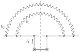
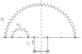
${\widehat{\text{II}\overline{\text{II}}}}$	${\widehat{\text{III}\overline{\text{I}}}}$	${\text{III}\overline{\text{I}}}$	${\text{IIF}\overline{\text{F}}}$

Figure 47: Graphs in which the gluons never connect $qg$ vertices in the initial state to vertices in the final state. It turns out that the 3 rightmost graphs have to be considered together for the correspondence with dipoles to work.

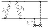
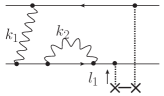
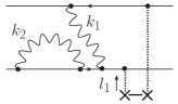
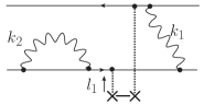
$\alpha_{1}$	$\alpha_{2}$	$\alpha_{3}$	$\alpha_{4}$

Figure 48: Dipoles graphs that correspond to the $p_{\perp}$-broadening graphs of Fig. 47. As usual, this set has to be supplemented by graphs exhausting all possible orderings of the vertices, including instantaneous exchanges. The leftmost graph corresponds to the leftmost graph in Fig. 47 while the set of the 3 rightmost graphs corresponds to the set of the 3 rightmost graphs in Fig. 47.

We now turn to a more tricky case, namely the 3 rightmost graphs in Fig. 47. These 3 graphs correspond to the 3 rightmost graphs in Fig. 48. Indeed, the sum of the energy denominators reads

$$\begin{split}\text{Re}\left(D_{\widehat{\text{III}\overline{\text{I}}}}+D_{\text{III}\overline{\text{I}}}+D_{\text{IIF}\overline{\text{F}}}\right)&=-\frac{1}{E_{1}^{2}E_{2}^{2}}-\frac{1}{E_{1}^{2}E_{2}(E_{1}+E_{2})}\\ &=-\text{Re}\sum\left(D_{\alpha_{2}}+D_{\alpha_{3}}+D_{\alpha_{4}}\right).\end{split}$$ (107)

It may look surprising that there is no graph-by-graph correspondence in this case, and especially that one needs to consider together purely initial-state graphs such as ${\widehat{\text{III}\overline{\text{I}}}}$ and a graph where one gluon is in the initial state and one in the final state (${\widehat{\text{IIF}\overline{\text{F}}}}$). However, we checked that not including the latter would lead to a mismatch between $p_{\perp}$-broadening and dipoles by a term $1/(2E_{1}^{3}E_{2})$.

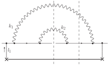
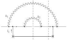
${\widehat{\text{FF}\overline{\text{FF}}}}$,${\widehat{\text{FFF}\overline{\text{F}}}}$	${\text{FFF}\overline{\text{F}}}$	${\widehat{\text{IF}\overline{\text{IF}}}}$,${\widehat{\text{IFF}\overline{\text{I}}}}$

Figure 49: Another set of graphs similar to Fig. 47 in correspondence with the dipole graphs in Fig. 48 or with similar graphs. One would also have the graphs in which the cut is on the left, symmetric to the rightmost cut.

We turn to the last class of graphs shown in Fig. 49. This case is solved by noting that these graphs may be mapped to the ones shown in Fig. 47, up to an analytical continuation in the $k_{2+}$ variable. We check the identities

$$D_{\widehat{\text{FF}\overline{\text{FF}}}}=D_{\widehat{\text{II}\overline{\text{II}}}}\ ,\ \ D_{\widehat{\text{FFF}\overline{\text{F}}}}+D_{\text{FFF}\overline{\text{F}}}+D_{\widehat{\text{IFF}\overline{\text{I}}}}\underset{\text{\tiny continuation in $k_{2+}$}}{\longleftrightarrow}D_{\text{III}\overline{\text{I}}}+D_{\widehat{\text{III}\overline{\text{I}}}}+D_{\text{IIF}\overline{\text{F}}}$$ (108)

and hence the corresponding identities with the (sets of) dipole graphs. Other graphs which we do not review here may be deduced from these ones by simple symmetries.

We have left out of the discussion a few graphs which are in exact one-to-one correspondence between the two processes. Up to these cases not discussed explicitly but trivial, the proof that the evolution with the energy of $p_{\perp}$-broadening cross sections and of dipole forward amplitudes is identical at next-to-leading order is now complete.

5 Extension to two-jet versus quadrupole amplitudes

The specific process on which we have focussed so far, namely $p_{\perp}$-broadening, is the simplest in the class of production processes. However, it is not the easiest to measure experimentally. Therefore, we wish to extend our analysis to other production processes.

It has been shown that quadrupole structures appear in the computation of observables which involve two particles (dijets) in the final state [24, 25, 26]. The energy evolution of quadrupoles can be related to the BFKL evolution with saturation, see Ref. [27] (approximation schemes were worked out in Ref. [28, 29]). The question is whether the dijet/quadrupole correspondence is true when quantum evolution is included.

The extension of our discussion of the evolution of $p_{\perp}$-broadening/dipole amplitudes to the evolution of dijet/quadrupole amplitudes is straightforward once one notices that the fermion vertices and energies entering the energy denominators never play any rôle. Indeed, the former are represented by a mere overall factor, which is identical for all graphs of a given class, and the latter do not even appear in the calculation, thanks to the soft approximation.

We illustrate the correspondence between two particular sets of graphs in Fig. 50 and 51, which are similar to Fig. 25 and 26 respectively. The relevant part of the dijet diagrams may be modeled by an incoming quark-antiquark dipole which subsequently evolves by gluon emission (Fig. 50).

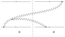
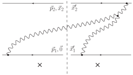
$A$	$B$

Figure 50: Two graphs contributing to the evolution of the dijet cross section. The incoming object is a $q\bar{q}$ dipole.

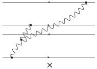
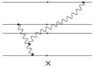
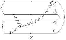
$\alpha$	$\beta$	$\gamma$

Figure 51: Quadrupole graphs corresponding to the dijet graphs of Fig. 50. On the rightmost graph, we have shown how the color lines close to form the quadrupole.

Let us denote by $\psi$ the wave function of the dipole, and $S_{4}$ the $S$-matrix element for the scattering of the quadrupole. Equation (1) is to be replaced by the following formula (see Fig. 50,51 for the notations):

$$\frac{dN}{d^{2}p_{1}d^{2}p_{2}}=\int\frac{d^{2}x^{\prime}_{1}d^{2}x_{2}d^{2}x^{\prime}_{2}}{(2\pi)^{2}}\psi(x_{2})\bar{\psi}(x^{\prime}_{2}-x_{1}^{\prime})e^{i\vec{p}_{1}\cdot\vec{x}^{\prime}_{1}-i\vec{p}_{2}\cdot(\vec{x}_{2}-\vec{x}^{\prime}_{2})}\\ \times S_{4}(0,x_{2},x^{\prime}_{2},x^{\prime}_{1}),$$ (109)

which now holds at next-to-leading order in the logarithms of the energy.

6 Conclusion

We have shown that the identity (1) between the amplitude for $p_{\perp}$-broadening and the dipole cross section holds at next-to-leading order level. The relation may be extended to dijet cross sections versus quadrupole amplitudes (Eq. (109)), and probably to other production processes. In other words, we have proved that the next-to-leading order BFKL equation describes the energy evolution of these production processes.

Our demonstration was based on a systematic (and quite awkward) inspection of all lightcone perturbation theory graphs which contribute to these respective processes. We have however avoided the full computation of the graphs since our goal was to prove the correspondence in the most general possible way.

The way the matching occurs turns out to be very subtle. In order to see it, we grouped the graphs according to their topologies (number of vertices of a given type, chronology of the different interactions) on the $p_{\perp}$-broadening side and on the dipole side. The time integrations for the dipole graphs are more constrained than for the $p_{\perp}$-broadening graphs (there are 4 independent integration regions in the latter case, and only 2 in the former case; see the discussion of the Keldysh-Schwinger formalism in Sec. 2). This first apparent mismatch is generally solved by subtle cancellations between graphs, and by considering appropriate ensembles of graphs (including, in particular, contact interactions where gluons are exchanged instantaneously, which turn out to play a crucial rôle). In some cases however, irreducible differences in the flow of longitudinal momenta result in differences in the energy denominators that can be resolved only by analytical continuation in the relevant longitudinal momentum variable. We found a number of pecularities: For example, keeping the consistency of the regularization (namely the adiabatic $\varepsilon$ parameter, see Eq. (18)) throughout the calculations turned out to be surprisingly important.

Despite our efforts, we have not found a simpler argument to explain the correspondence more systematically. Such an argument would be crucial for example to be able to understand whether the correspondence is still true at next-to-next-to-leading order and beyond.

A full next-to-leading order calculation of production processes requires also to take into account the next-to-leading order corrections to the parton distribution functions and to the fragmentation functions. In particular, one has to release the eikonal approximation at the quark-gluon vertices, which we have not done here. Progress in this direction has recently been reported, see Ref. [30, 31]: In these respects, our work may be seen as complementary to the latter studies.

References

- [1] D. Kharzeev, E. Levin and L. McLerran, Nucl. Phys. A 748, 627 (2005) [hep-ph/0403271].
- [2] C. Marquet, Nucl. Phys. A 796, 41 (2007) [arXiv:0708.0231 [hep-ph]].
- [3] J. L. Albacete and C. Marquet, Phys. Rev. Lett. 105, 162301 (2010) [arXiv:1005.4065 [hep-ph]].
- [4] L. N. Lipatov, Sov. J. Nucl. Phys. 23, 338 (1976) [Yad. Fiz. 23, 642 (1976)].
- [5] E. A. Kuraev, L. N. Lipatov and V. S. Fadin, Sov. Phys. JETP 45, 199 (1977) [Zh. Eksp. Teor. Fiz. 72, 377 (1977)].
- [6] I. I. Balitsky and L. N. Lipatov, Sov. J. Nucl. Phys. 28, 822 (1978) [Yad. Fiz. 28, 1597 (1978)].
- [7] M. Ciafaloni and G. Camici, Phys. Lett. B 430, 349 (1998) [hep-ph/9803389].
- [8] V. S. Fadin and L. N. Lipatov, Phys. Lett. B 429, 127 (1998) [hep-ph/9802290].
- [9] M. Ciafaloni, D. Colferai, G. P. Salam and A. M. Stasto, JHEP 0708, 046 (2007) [arXiv:0707.1453 [hep-ph]].
- [10] G. Altarelli, R. D. Ball and S. Forte, Nucl. Phys. B 799, 199 (2008) [arXiv:0802.0032 [hep-ph]].
- [11] B. G. Zakharov, JETP Lett. 63, 952 (1996) [hep-ph/9607440].
- [12] Y. V. Kovchegov and K. Tuchin, Phys. Rev. D 65, 074026 (2002) [hep-ph/0111362].
- [13] A. H. Mueller, Nucl. Phys. B 415, 373 (1994).
- [14] G. P. Lepage and S. J. Brodsky, Phys. Rev. D 22, 2157 (1980).
- [15] Z. Chen and A. H. Mueller, Nucl. Phys. B 451, 579 (1995).
- [16] L. D. McLerran and R. Venugopalan, Phys. Rev. D 49, 2233 (1994) [hep-ph/9309289].
- [17] L. V. Keldysh, Zh. Eksp. Teor. Fiz. 47, 1515 (1964) [Sov. Phys. JETP 20, 1018 (1965)].
- [18] J. S. Schwinger, J. Math. Phys. 2, 407 (1961).
- [19] F. Gelis and R. Venugopalan, Nucl. Phys. A 776, 135 (2006) [hep-ph/0601209].
- [20] J. Jalilian-Marian and Y. V. Kovchegov, Prog. Part. Nucl. Phys. 56, 104 (2006) [hep-ph/0505052].
- [21] D. Kharzeev, Y. V. Kovchegov and K. Tuchin, Phys. Rev. D 68, 094013 (2003) [hep-ph/0307037].
- [22] Y. V. Kovchegov and H. Weigert, Nucl. Phys. A 807, 158 (2008) [arXiv:0712.3732 [hep-ph]].
- [23] Y. V. Kovchegov and H. Weigert, Nucl. Phys. A 784, 188 (2007) [hep-ph/0609090].
- [24] J. Jalilian-Marian and Y. V. Kovchegov, Phys. Rev. D 70, 114017 (2004) [Erratum-ibid. D 71, 079901 (2005)] [hep-ph/0405266].
- [25] F. Dominguez, B. -W. Xiao and F. Yuan, Phys. Rev. Lett. 106, 022301 (2011) [arXiv:1009.2141 [hep-ph]].
- [26] F. Dominguez, C. Marquet, B. -W. Xiao and F. Yuan, Phys. Rev. D 83, 105005 (2011) [arXiv:1101.0715 [hep-ph]].
- [27] F. Dominguez, A. H. Mueller, S. Munier and B. -W. Xiao, Phys. Lett. B 705, 106 (2011) [arXiv:1108.1752 [hep-ph]].
- [28] E. Iancu and D. N. Triantafyllopoulos, JHEP 1111, 105 (2011) [arXiv:1109.0302 [hep-ph]].
- [29] E. Iancu and D. N. Triantafyllopoulos, JHEP 1204, 025 (2012) [arXiv:1112.1104 [hep-ph]].
- [30] G. A. Chirilli, B. -W. Xiao and F. Yuan, Phys. Rev. Lett. 108, 122301 (2012) [arXiv:1112.1061 [hep-ph]].
- [31] G. A. Chirilli, B. -W. Xiao and F. Yuan, arXiv:1203.6139 [hep-ph].
- [32] D. Binosi and L. Theussl, Comput. Phys. Commun. 161, 76 (2004) [hep-ph/0309015].
- [33] D. Binosi, J. Collins, C. Kaufhold and L. Theussl, Comput. Phys. Commun. 180, 1709 (2009) [arXiv:0811.4113 [hep-ph]].