Geometrical structure of Laplacian eigenfunctions

Abstract

We summarize the properties of eigenvalues and eigenfunctions of the Laplace operator in bounded Euclidean domains with Dirichlet, Neumann or Robin boundary condition. We keep the presentation at a level accessible to scientists from various disciplines ranging from mathematics to physics and computer sciences. The main focus is put onto multiple intricate relations between the shape of a domain and the geometrical structure of eigenfunctions.

Dedicated to Professor Bernard Sapoval for his 75th birthday

1 Introduction

This review focuses on the classical eigenvalue problem for the Laplace operator $\Delta=\partial^{2}/\partial x_{1}^{2}+...+\partial^{2}/\partial x_{d}^{2}$ in an open bounded connected domain $\Omega\subset{\mathbb{R}}^{d}$ ($d=2,3,...$ being the space dimension),

$$-\Delta u_{m}(x)=\lambda_{m}u_{m}(x)\quad(x\in\Omega),$$ (1)

with Dirichlet, Neumann or Robin boundary condition on a piecewise smooth boundary ${\partial\Omega}$:

$$\begin{split}u_{m}(x)&=0\quad(x\in{\partial\Omega})\quad\mathrm{(Dirichlet)},\\ \frac{\partial}{\partial n}u_{m}(x)&=0\quad(x\in{\partial\Omega})\quad\mathrm{(Neumann)},\\ \frac{\partial}{\partial n}u_{m}(x)+hu_{m}(x)&=0\quad(x\in{\partial\Omega})\quad\mathrm{(Robin)},\\ \end{split}$$ (2)

where $\partial/\partial n$ is the normal derivative pointed outwards the domain, and $h$ is a positive constant. The spectrum of the Laplace operator is known to be discrete, the eigenvalues $\lambda_{m}$ are nonnegative and ordered in an ascending order by the index $m=1,2,3,...$,

$$(0\leq)\lambda_{1}<\lambda_{2}\leq\lambda_{3}\leq\ldots\nearrow\infty$$ (3)

(with possible multiplicities), while the eigenfunctions $\{u_{m}(x)\}$ form a complete basis in the functional space $L_{2}(\Omega)$ of measurable and square-integrable functions on $\Omega$ [138, 421]. By definition, the function $0$ satisfying Eqs. (1, 2) is excluded from the set of eigenfunctions. Since the eigenfunctions are defined up to a multiplicative factor, it is sometimes convenient to normalize them to get the unit $L_{2}$-norm:

$$\|u_{m}\|_{2}\equiv\|u_{m}\|_{L_{2}(\Omega)}\equiv\left(\int\limits_{\Omega}dx~{}|u_{m}(x)|^{2}\right)^{1/2}=1$$ (4)

(note that there is still ambiguity up to the multiplication by $e^{i\alpha}$, with $\alpha\in{\mathbb{R}}$).

Laplacian eigenfunctions appear as vibration modes in acoustics, as electron wave functions in quantum waveguides, as natural basis for constructing heat kernels in the theory of diffusion, etc. For instance, vibration modes of a thin membrane (a drum) with a fixed boundary are given by Dirichlet Laplacian eigenfunctions $u_{m}$, with the drum frequencies proportional to $\sqrt{\lambda_{m}}$ [418]. A particular eigenmode can be excited at the corresponding frequency [442, 443, 444]. In the theory of diffusion, an interpretation of eigenfunctions is less explicit. The first eigenfunction represents the long-time asymptotic spatial distribution of particles diffusing in a bounded domain (see below). A conjectural probabilistic representation of higher-order eigenfunctions through a Fleming-Viot type model was developed by Burdzy et al. [101, 103].

The eigenvalue problem (1, 2) is archetypical in the theory of elliptic operators, while the properties of the underlying eigenfunctions have been thoroughly investigated in various mathematical and physical disciplines, including spectral theory, probability and stochastic processes, dynamical systems and quantum billiards, condensed matter physics and quantum mechanics, theory of acoustical, optical and quantum waveguides, computer sciences, etc. Many books and reviews were dedicated to different aspects of Laplacian eigenvalues, eigenfunctions and their applications (see, e.g., [390, 401, 36, 243, 300, 125, 147, 165, 254, 27, 226, 29, 11, 58]). The diversity of notions and methods developed by mathematicians, physicists and computer scientists often makes the progress in one discipline almost unknown or hardly accessible to scientists from the other disciplines. One of the goals of the review is to bring together various facts about Laplacian eigenvalues and eigenfunctions and to present them at a level accessible to scientists from various disciplines. For this purpose, many technical details and generalities are omitted in favor to simple illustrations. While the presentation is focused on the Laplace operator in bounded Euclidean domains with piecewise smooth boundaries, a number of extensions are relatively straightforward. For instance, the Laplace operator can be extended to a second order elliptic operator with appropriate coefficients, the piecewise smoothness of a boundary can often be relaxed [329, 219], while Euclidean domains can be replaced by Riemannian manifolds or weighted graphs [254]. The main emphasis is put onto the geometrical structure of Laplacian eigenfunctions and on their relation to the shape of a domain. Although the bibliography counts more than five hundred citations, it is far from being complete, and readers are invited to refer to other reviews and books for further details and references.

The review is organized as follows. We start by recalling in Sec. 2 general properties of the Laplace operator. Explicit representations of eigenvalues and eigenfunctions in simple domains are summarized in Sec. 3. In Sec. 4 we review the properties of eigenvalues and their relation to the shape of a domain: Weyl’s asymptotic law, isoperimetric inequalities and the related shape optimization problems, and Kac’s inverse spectral problem. Although eigenfunctions are not involved at this step, valuable information can be learned about the domain from the eigenvalues alone. The next step consists in the analysis of nodal lines/surfaces or nodal domains in Sec. 5. The nodal lines tell us how the zeros of eigenfunctions are spatially distributed, while their amplitudes are still ignored. In Sec. 6, several estimates for the amplitudes of eigenfunctions are summarized. Most of these results were obtained during the last twenty years.

Section 7 is devoted to the property of eigenfunctions known as localization. We start by recalling the notion of localization in quantum mechanics: the strong localization by a potential (Sec. 7.1), Anderson localization (Sec. 7.2) and trapped modes in infinite waveguides (Sec. 7.3). In all three cases, the eigenvalue problem is different from Eqs. (1, 2), due to either the presence of a potential, or the unboundness of a domain. Nevertheless, these cases are instructive, as similar effects may be observed for the eigenvalue problem (1, 2). In particular, we discuss in Sec. 7.4 an exponentially decaying upper bound for the norm of eigenfunctions in domains with branches of variable cross-sectional profiles. Section 7.5 reviews the properties of low-frequency eigenfunctions in “dumbbell” domains, in which two (or many) subdomains are connected by narrow channels. This situation is convenient for a rigorous analysis as the width of channels plays the role of a small parameter [440]. A number of asymptotic results for eigenvalues and eigenfunctions were derived, for Dirichlet, Neumann and Robin boundary conditions. A harder case of irregular or fractal domains is discussed in Sec. 7.6. Here, it is difficult to identify a relevant small parameter to get rigorous estimates. In spite of numerous numerical examples of localized eigenfunctions (both for Dirichlet and Neumann boundary conditions), a comprehensive theory of localization is still missing. Section 7.7 is devoted to high-frequency localization and the related scarring problems in quantum billiards. We start by illustrating the classical whispering gallery, bouncing ball and focusing modes in circular and elliptical domains. We also provide examples for the case without localization. A brief overview of quantum billiards is presented. In the last Sec. 8, we mention some issues that could not be included into the review, e.g., numerical methods for computation of eigenfunctions or their numerous applications.

2 Basic properties

We start by recalling basic properties of the Laplacian eigenvalues and eigenfunctions (see [138, 421, 71] or other standard textbooks).

(i) The eigenfunctions are infinitely differentiable inside the domain $\Omega$. For any open subset $V\subset\Omega$, the restriction of $u_{m}$ on $V$ cannot be strictly $0$ [300].

(ii) Multiplying Eq. (1) by $u_{m}$, integrating over $\Omega$ and using the Green’s formula yield

$$\lambda_{m}=\frac{\int\limits_{\Omega}dx~{}|\nabla u_{m}|^{2}-\int\limits_{{\partial\Omega}}dx~{}u_{m}\frac{\partial u_{m}}{\partial n}}{\int\limits_{\Omega}dx~{}u_{m}^{2}}=\frac{\|\nabla u_{m}\|_{L_{2}(\Omega)}^{2}+h\|u_{m}\|_{L_{2}({\partial\Omega})}^{2}}{\|u_{m}\|_{L_{2}(\Omega)}^{2}},$$ (5)

where $\nabla$ stands for the gradient operator, and we used Robin boundary condition (2) in the last equality; for Dirichlet or Neumann boundary conditions, the boundary integral (second term) vanishes. This formula ensures that all eigenvalues are nonnegative.

(iii) Similar expression appears in the variational formulation of the eigenvalue problem, known as the minimax principle [138]

$$\lambda_{m}=\min\max\frac{\|\nabla v\|_{L_{2}(\Omega)}^{2}+h\|v\|_{L_{2}({\partial\Omega})}^{2}}{\|v\|_{L_{2}(\Omega)}^{2}},$$ (6)

where the maximum is over all linear combinations of the form

$$v=a_{1}\phi_{1}+...+a_{m}\phi_{m},$$

and the minimum is over all choices of $m$ linearly independent continuous and piecewise-differentiable functions $\phi_{1}$, …, $\phi_{m}$ (said to be in the Sobolev space $H^{1}(\Omega)$) [138, 238]. Note that the minimum is reached exactly on the eigenfunction $u_{m}$. For Dirichlet eigenvalue problem, there is a supplementary condition $v=0$ on the boundary ${\partial\Omega}$ so that the second term in Eq. (6) is canceled. For Neumann eigenvalue problem, $h=0$ and the second term vanishes again.

(iv) The minimax principle implies the monotonous increase of the eigenvalues $\lambda_{m}$ with $h$, namely if $h<h^{\prime}$, then $\lambda_{m}(h)\leq\lambda_{m}(h^{\prime})$. In particular, any eigenvalue $\lambda_{m}(h)$ of the Robin problem lies between the corresponding Neumann and Dirichlet eigenvalues.

(v) For Dirichlet boundary condition, the minimax principle implies the property of domain monotonicity: eigenvalues monotonously decrease when the domain enlarges, i.e., $\lambda_{m}(\Omega_{1})\geq\lambda_{m}(\Omega_{2})$ if $\Omega_{1}\subset\Omega_{2}$. This property does not hold for Neumann or Robin boundary conditions, as illustrated by a simple counter-example on Fig. 1.

Fig. 1: A counter-example for the property of domain monotonicity for Neumann boundary condition. Although a smaller rectangle $\Omega_{1}$ is inscribed into a larger rectangle $\Omega_{2}$ (i.e., $\Omega_{1}\subset\Omega_{2}$), the second eigenvalue $\lambda_{2}(\Omega_{1})=\pi^{2}/c^{2}$ is smaller than the second eigenvalue $\lambda_{2}(\Omega_{2})=\pi^{2}/a^{2}$ (if $a>b$) when $c=\sqrt{(a-\alpha)^{2}+(b-\beta)^{2}}>a$ (courtesy by N. Saito; see also [238], Sec. 1.3.2).

(vi) The eigenvalues are invariant under translations and rotations of the domain. This is a key property for an efficient image recognition and analysis [424, 436, 437]. When a domain is expanded by factor $\alpha$, all the eigenvalues are rescaled by $1/\alpha^{2}$.

(vii) The first eigenfunction $u_{1}$ does not change the sign and can be chosen positive. Because of the orthogonality of eigenfunctions, $u_{1}$ is in fact the only eigenfunction not changing its sign.

(viii) The first eigenvalue $\lambda_{1}$ is simple and strictly positive for Dirichlet and Robin boundary conditions; for Neumann boundary condition, $\lambda_{1}=0$ and $u_{1}$ is a constant.

(ix) The completeness of eigenfunctions in $L_{2}(\Omega)$ can be expressed as

$$\sum\limits_{m}u_{m}(x)u_{m}^{*}(y)=\delta(x-y)\qquad(x,y\in\Omega),$$ (7)

where asterisk denotes the complex conjugate, $\delta(x)$ is the Dirac distribution, and the eigenfunctions are $L_{2}$-normalized. Multiplying this relation by a function $f\in L_{2}(\Omega)$ and integrating over $\Omega$ yields the decomposition of $f(x)$ over $u_{m}(x)$:

$$f(x)=\sum\limits_{m}u_{m}(x)\int\limits_{\Omega}dy~{}f(y)~{}u_{m}^{*}(y).$$

(x) The Green function $G(x,y)$ for the Laplace operator which satisfies

$$-\Delta G(x,y)=\delta(x-y)\qquad(x,y\in\Omega)$$ (8)

(with an appropriate boundary condition), admits the spectral decomposition over the $L_{2}$-normalized eigenfunctions

$$G(x,y)=\sum\limits_{m}\lambda_{m}^{-1}u_{m}(x)u_{m}^{*}(y).$$ (9)

(for Neumann boundary condition, $\lambda_{1}=0$ has to be excluded; in that case, the Green function is defined up to an additive constant).

Similarly, the heat kernel (or diffusion propagator) $G_{t}(x,y)$ satisfying

$$\begin{split}\frac{\partial}{\partial t}G_{t}(x,y)-\Delta G_{t}(x,y)&=0\qquad(x,y\in\Omega),\\ G_{t=0}(x,y)&=\delta(x-y)\\ \end{split}$$ (10)

(with an appropriate boundary condition), admits the spectral decomposition

$$G_{t}(x,y)=\sum\limits_{m}e^{-\lambda_{m}t}u_{m}(x)u_{m}^{*}(y).$$ (11)

The Green function and heat kernel allow one to solve the standard boundary value and Cauchy problems for the Laplace and heat equations, respectively [139, 118]. The decompositions (9, 11) are the major tool for getting explicit solutions in simple domains for which the eigenfunctions are known explicitly (see Sec. 3). This representation is also important for the theory of diffusion due to the probabilistic interpretation of $G_{t}(x,y)dx$ as the conditional probability for Brownian motion started at $y$ to arrive in the $dx$ vicinity of $x$ after a time $t$ [177, 51, 52, 202, 420, 249, 500, 406, 84]. Setting Dirichlet, Neumann or Robin boundary conditions, one can respectively describe perfect absorptions, perfect reflections and partial absorption/reflection on the boundary [212].

For Dirichlet boundary condition, if $\Omega\subset\Omega^{\prime}$, then $0\leq G_{t}^{(\Omega)}(x,y)\leq G_{t}^{(\Omega^{\prime})}(x,y)$ [490]. In particular, taking $\Omega^{\prime}={\mathbb{R}}^{d}$, one gets

$$0\leq G_{t}(x,y)\leq(4\pi t)^{-d/2}\exp\left(-\frac{|x-y|^{2}}{4t}\right),$$ (12)

where the Gaussian heat kernel for free space is written on the right-hand side. The above domain monotonicity for heat kernels may not hold for Neumann boundary condition [53].

(xi) For Dirichlet boundary condition, the eigenvalues vary continuously under a “continuous” perturbation of the domain [138]. For Neumann boundary condition, the situation is much more delicate. The continuity still holds when a bounded domain with a smooth boundary is deformed by a “continuously differentiable transformation”, while in general this statement is false, with an explicit counter-example provided in [138]. Note that the continuity of the spectrum is important for numerical computations of the eigenvalues by finite element or other methods, in which an irregular boundary is replaced by a suitable polygonal or piecewise smooth approximation. The underlying assumption that the eigenvalues are very little affected by such domain perturbations, holds in great generality for Dirichlet boundary condition, but is much less evident for Neumann boundary condition [105]. The spectral stability of elliptic operators under domain perturbations has been thoroughly investigated [226, 240, 105, 106, 107, 108, 109]. It is also worth stressing that the spectrum of the Laplace operator in a bounded domain with Neumann boundary condition on an irregular boundary may not be discrete, with explicit counter-examples provided in [237].

3 Eigenbasis for simple domains

We list the examples of “simple” domains, in which symmetries allow for variable separations and thus explicit representations of eigenfunctions in terms of elementary or special functions.

3.1 Intervals, rectangles, parallelepipeds

For rectangle-like domains $\Omega=[0,\ell_{1}]\times...\times[0,\ell_{d}]\subset{\mathbb{R}}^{d}$ (with the sizes $\ell_{i}>0$), the natural variable separation yields

$$\begin{split}u_{n_{1},...,n_{d}}(x_{1},...,x_{d})&=u_{n_{1}}^{(1)}(x_{1})\ldots u_{n_{d}}^{(d)}(x_{d}),\qquad\lambda_{n_{1},...,n_{d}}=\lambda_{n_{1}}^{(1)}+...+\lambda_{n_{d}}^{(d)},\\ \end{split}$$ (13)

where the multiple index $n_{1}...n_{d}$ is used instead of $m$, and $u_{n_{i}}^{(i)}(x_{i})$ and $\lambda_{n_{i}}^{(i)}$ ($i=1,...,d$) correspond to the one-dimensional problem on the interval $[0,\ell_{i}]$. Depending on the boundary condition, $u_{n}^{(i)}(x)$ are sines (Dirichlet), cosines (Neumann) or their combinations (Robin):

$$\begin{split}u_{n}^{(i)}(x)&=\sin(\pi(n+1)x/\ell_{i}),\quad\lambda_{n}^{(i)}=\pi^{2}(n+1)^{2}/\ell_{i}^{2},\hskip 28.45274pt\rm{(Dirichlet)},\\ u_{n}^{(i)}(x)&=\cos(\pi nx/\ell_{i}),\hskip 34.1433pt\lambda_{n}^{(i)}=\pi^{2}n^{2}/\ell_{i}^{2},\hskip 54.06023pt\rm{(Neumann)},\\ u_{n}^{(i)}(x)&=\sin(\alpha_{n}x/\ell_{i})+\frac{\alpha_{n}}{h\ell_{i}}\cos(\alpha_{n}x/\ell_{i}),\quad\lambda_{n}^{(i)}=\alpha_{n}^{2}/\ell_{i}^{2},\hskip 8.53581pt\rm{(Robin)},\\ \end{split}$$ (14)

where $n=0,1,2,...$ and the coefficients $\alpha_{n}$ depend on the parameter $h$ and satisfy the equation obtained by imposing the Robin boundary condition in Eq. (2) at $x=\ell_{i}$:

$$\frac{2\alpha_{n}}{h\ell_{i}}\cos\alpha_{n}+\left(1-\frac{\alpha_{n}^{2}}{h^{2}\ell_{i}^{2}}\right)\sin\alpha_{n}=0.$$ (15)

According to the property (iv) of Sec. 2, this equation has the unique solution $\alpha_{n}$ on each interval $[n\pi,(n+1)\pi]$ ($n=0,1,2,...$), that makes its numerical computation by bisection (or other) method easy and fast. All the eigenvalues $\lambda_{n}^{(i)}$ are simple (not degenerate), while

$$\|u_{n}^{(i)}(x)\|_{L_{2}((0,\ell_{i}))}=\left(\frac{\alpha_{n}^{2}+2h\ell_{i}+h^{2}\ell_{i}^{2}}{2h^{2}}\right)^{1/2}.$$ (16)

In turn, the eigenvalues $\lambda_{n_{1},...,n_{d}}$ can be degenerate if there exists a rational ratio $(\ell_{i}/\ell_{j})^{2}$ (with $i\neq j$). For instance, the first Dirichlet eigenvalues of the unit square are $2\pi^{2}$, $5\pi^{2}$, $5\pi^{2}$, $8\pi^{2}$, …. , with the twice degenerate second eigenvalue. An eigenfunction associated to a degenerate eigenvalue is a linear combination of the corresponding functions. For the above example $u(x_{1},x_{2})=c_{1}\sin(\pi x_{1})\sin(2\pi x_{2})+c_{2}\sin(2\pi x_{1})\sin(\pi x_{2})$ with any $c_{1}$ and $c_{2}$ such that $c_{1}^{2}+c_{2}^{2}\neq 0$.

3.2 Disk, sector and circular annulus

The rotation symmetry of a circular annulus, $\Omega=\{x\in{\mathbb{R}}^{2}~{}:~{}R_{0}<|x|<R\}$, allows one to write the Laplace operator in polar coordinates,

$$\begin{cases}x_{1}=r\cos\varphi,\cr x_{2}=r\sin\varphi,\end{cases}\qquad\Delta=\frac{\partial^{2}}{\partial r^{2}}+\frac{1}{r}\frac{\partial}{\partial r}+\frac{1}{r^{2}}\frac{\partial^{2}}{\partial\varphi^{2}},$$ (17)

that leads to variable separation and an explicit representation of eigenfunctions

$$u_{nkl}(r,\varphi)=\bigl{[}J_{n}(\alpha_{nk}r/R)+c_{nk}Y_{n}(\alpha_{nk}r/R)\bigr{]}\times\begin{cases}\cos(n\varphi),\quad l=1,\cr\sin(n\varphi),\quad l=2~{}(n\neq 0),\end{cases}$$ (18)

where $J_{n}(z)$ and $Y_{n}(z)$ are the Bessel functions of the first and second kind [1, 498, 86], and the coefficients $\alpha_{nk}$ and $c_{nk}$ are set by the boundary conditions at $r=R$ and $r=R_{0}$:

$$\begin{split}0&=\frac{\alpha_{nk}}{R}\biggl{[}J^{\prime}_{n}(\alpha_{nk})+c_{nk}Y^{\prime}_{n}(\alpha_{nk})\biggr{]}+h\biggl{[}J_{n}(\alpha_{nk})+c_{nk}Y_{n}(\alpha_{nk})\biggr{]},\\ 0&=-\frac{\alpha_{nk}}{R}\biggl{[}J^{\prime}_{n}\bigl{(}\alpha_{nk}\frac{R_{0}}{R}\bigr{)}+c_{nk}Y^{\prime}_{n}\bigl{(}\alpha_{nk}\frac{R_{0}}{R}\bigr{)}\biggr{]}+h\biggl{[}J_{n}\bigl{(}\alpha_{nk}\frac{R_{0}}{R}\bigr{)}+c_{nk}Y_{n}\bigl{(}\alpha_{nk}\frac{R_{0}}{R}\bigr{)}\biggr{]}.\\ \end{split}$$ (19)

For each $n=0,1,2,...$, the system of these equations has infinitely many solutions $\alpha_{nk}$ which are enumerated by the index $k=1,2,3,...$ [498]. The eigenfunctions are enumerated by the triple index $nkl$, with $n=0,1,2,...$ counting the order of Bessel functions, $k=1,2,3,...$ counting solutions of Eqs. (19), and $l=1,2$. Since $u_{0k2}(r,\varphi)$ are trivially zero (as $\sin(n\varphi)=0$ for $n=0$), they are excluded. The eigenvalues $\lambda_{nk}=\alpha_{nk}^{2}/R^{2}$, which are independent of the last index $l$, are simple for $n=0$ and twice degenerate for $n>0$. In the latter case, an eigenfunction is any nontrivial linear combination of $u_{nk1}$ and $u_{nk2}$. The squared $L_{2}$-norm of the eigenfunction is

$$\begin{split}\|u_{nkl}(r,\varphi)\|_{2}^{2}=\frac{\pi(2-\delta_{n,0})R^{2}}{2\alpha_{nk}^{2}}\biggl{[}&\biggl{(}\alpha_{nk}^{2}+h^{2}R^{2}-n^{2}\biggr{)}v_{nk}^{2}(R)\\ &-\biggl{(}(\alpha_{nk}^{2}+h^{2}R^{2})\frac{R_{0}^{2}}{R^{2}}-n^{2}\biggr{)}v_{nk}^{2}(R_{0})\biggr{]},\\ \end{split}$$ (20)

where $v_{nk}(r)=J_{n}(\alpha_{nk}r/R)+c_{nk}Y_{n}(\alpha_{nk}r/R)$.

For the special case of a disk ($R_{0}=0$), all the coefficients $c_{nk}$ in front of the Bessel functions $Y_{n}(z)$ (divergent at $0$) are set to $0$:

$$u_{nkl}(r,\varphi)=J_{n}(\alpha_{nk}r/R)\times\begin{cases}\cos(n\varphi),\quad l=1,\cr\sin(n\varphi),\quad l=2~{}(n\neq 0),\end{cases}$$ (21)

where $\alpha_{nk}$ are either the positive roots $j_{nk}$ of the Bessel function $J_{n}(z)$ (Dirichlet), or the positive roots $\tilde{j}_{nk}$ of its derivative $J^{\prime}_{n}(z)$ (Neumann), or the positive roots of their linear combination $J^{\prime}_{n}(z)+hJ_{n}(z)$ (Robin). The asymptotic behavior of zeros of Bessel functions was thoroughly investigated. For fixed $k$ and large $n$, the Olver’s expansion holds $j_{nk}\simeq n+\delta_{k}n^{1/3}+O(n^{-1/3})$ (with known coefficients $\delta_{k}$) [377, 378, 166], while for fixed $n$ and large $k$, the McMahon’s expansion holds: $j_{nk}\simeq\pi(k+n/2-1/4)+O(k^{-1})$ [498]. Similar asymptotic relations are applicable for Neumann and Robin boundary conditions.

For a circular sector of radius $R$ and of angle $\pi\beta$, the eigenfunctions are

$$u_{nk}(r,\varphi)=J_{n/\beta}(\alpha_{nk}r/R)\times\begin{cases}\sin(n\varphi/\beta)\quad\textrm{(Dirichlet)}\cr\cos(n\varphi/\beta)\quad\textrm{(Neumann)}\end{cases}\quad(r<R,~{}0<\varphi<\pi\beta)$$ (22)

i.e., they are expressed in terms of Bessel functions of fractional order, and $\alpha_{nk}$ are the positive roots of $J_{n/\beta}(z)$ (Dirichlet) or $J^{\prime}_{n/\beta}(z)$ (Neumann). The Robin boundary condition and a sector of a circular annulus can be treated similarly.

3.3 Sphere and spherical shell

The rotation symmetry of a spherical shell in three dimensions, $\Omega=\{x\in{\mathbb{R}}^{3}~{}:~{}R_{0}<|x|<R\}$, allows one to write the Laplace operator in spherical coordinates,

$$\begin{cases}x_{1}=r\sin\theta\cos\varphi,\cr x_{2}=r\sin\theta\sin\varphi,\cr x_{3}=r\cos\theta,\cr\end{cases}\qquad\Delta=\frac{\partial^{2}}{\partial r^{2}}+\frac{2}{r}\frac{\partial}{\partial r}+\frac{1}{r^{2}}\left(\frac{1}{\sin\theta}\frac{\partial}{\partial\theta}\sin\theta\frac{\partial}{\partial\theta}+\frac{\partial^{2}}{\partial\varphi^{2}}\right),$$ (23)

that leads to the variable separation and an explicit representation of eigenfunctions

$$u_{nkl}(r,\theta,\varphi)=\bigl{[}j_{n}(\alpha_{nk}r/R)+c_{nk}y_{n}(\alpha_{nk}r/R)\bigr{]}P_{n}^{l}(\cos\theta)e^{il\varphi},$$ (24)

where $j_{n}(z)$ and $y_{n}(z)$ are the spherical Bessel functions of the first and second kind,

$$j_{n}(z)=\sqrt{\frac{\pi}{2z}}J_{n+1/2}(z),\qquad y_{n}(z)=\sqrt{\frac{\pi}{2z}}Y_{n+1/2}(z),$$ (25)

$P_{n}^{l}(z)$ are associated Legendre polynomials (note that the angular part, $P_{n}^{l}(\cos\theta)e^{il\varphi}$, is also called spherical harmonic and denoted as $Y_{nl}(\theta,\varphi)$, up to a normalization factor). The coefficients $\alpha_{nk}$ and $c_{nk}$ are set by the boundary conditions at $r=R$ and $r=R_{0}$ similar to Eq. (19). The eigenfunctions are enumerated by the triple index $nkl$, with $n=0,1,2,...$ counting the order of spherical Bessel functions, $k=1,2,3,...$ counting zeros, and $l=-n,-n+1,...,n$. The eigenvalues $\lambda_{nk}=\alpha_{nk}^{2}/R^{2}$, which are independent of the last index $l$, have the degeneracy $2n+1$. The squared $L_{2}$-norm of the eigenfunction is

$$\begin{split}\|u_{nkl}(r,\theta,\varphi)\|_{2}^{2}&=\frac{2\pi R^{3}}{(2n+1)\alpha_{nk}^{2}}\biggl{[}\biggl{(}\alpha_{nk}^{2}+h^{2}R^{2}-hR-n(n+1)\biggr{)}v_{nk}^{2}(R)\\ &-\biggl{(}\alpha_{nk}^{2}(R_{0}/R)^{3}+h^{2}R_{0}^{2}-hR_{0}-n(n+1)R_{0}/R\biggr{)}v_{nk}^{2}(R_{0})\biggr{]},\\ \end{split}$$ (26)

where $v_{nk}(r)=j_{n}(\alpha_{nk}r/R)+c_{nk}y_{n}(\alpha_{nk}r/R)$.

In the special case of a sphere ($R_{0}=0$), one has $c_{nk}=0$ and the equations are simplified. For balls and spherical shells in higher dimensions ($d>3$), the radial dependence of eigenfunctions is expressed through a linear combination of so-called ultra-spherical Bessel functions $r^{1-d/2}J_{\frac{d}{2}-1+n}(\alpha_{nk}r/R)$ and $r^{1-d/2}Y_{\frac{d}{2}-1+n}(\alpha_{nk}r/R)$.

3.4 Ellipse and elliptical annulus

In elliptic coordinates, the Laplace operator reads as

$$\begin{cases}x_{1}=a\cosh r\cos\theta,\cr x_{2}=a\sinh r\sin\theta,\end{cases}\hskip 28.45274pt\Delta=\frac{1}{a^{2}(\sinh^{2}r+\sin^{2}\theta)}\left(\frac{\partial^{2}}{\partial r^{2}}+\frac{\partial^{2}}{\partial\theta^{2}}\right),$$ (27)

where $a>0$ is the prescribed distance between the origin and the foci, $r\geq 0$ and $0\leq\theta<2\pi$ are the radial and angular coordinates (Fig. 2). An ellipse is a curve of constant $r=R$ so that its points $(x_{1},x_{2})$ satisfy $x_{1}^{2}/A^{2}+x_{2}^{2}/B^{2}=1$, where $R$ is the “radius” of the ellipse and $A=a\cosh R$ and $B=a\sinh R$ are the major and minor semi-axes. Note that the eccentricity $e=a/A=1/\cosh R$ is strictly positive. A filled ellipse (i.e., the interior of an given ellipse) can be characterized in elliptic coordinates as $0\leq r<R$ and $0\leq\theta<2\pi$. Similarly, an elliptical annulus (i.e., the interior between two ellipses with the same foci) is characterized by $R_{0}<r<R$ and $0\leq\theta<2\pi$.

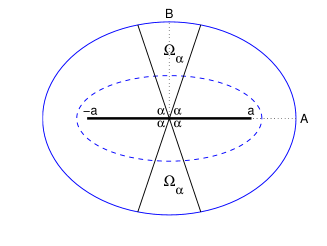
Fig. 2: Two ellipses of radii $R=0.5$ (dashed line) and $R=1$ (solid line), with the focal distance $a=1$. The major and minor semi-axes, $A=a\cosh R$ and $B=a\sinh R$, are shown by black dotted lines. The horizontal thick segment connects the foci.

In the elliptic coordinates, the variables can be separated, $u(r,\theta)=f(r)g(\theta)$, from which Eq. (1) reads as

$$\left(\frac{1}{f(r)}\frac{d^{2}f}{dr^{2}}+\frac{\lambda a^{2}}{2}\cosh(2r)\right)=-\left(\frac{1}{g(\theta)}\frac{d^{2}g}{d\theta^{2}}-\frac{\lambda a^{2}}{2}\cos(2\theta)\right)$$

so that both sides are equal to a constant (denoted $c$). As a consequence, the angular and radial parts, $g(\theta)$ and $f(r)$, are solutions of the Mathieu equation and the modified Mathieu equation, respectively [352, 513, 126]

$$g^{\prime\prime}(\theta)+\left(c-2q\cos 2\theta\right)g(\theta)=0,\qquad f^{\prime\prime}(r)-\left(c-2q\cosh 2r\right)f(r)=0,$$

where $q=\lambda a^{2}/4$ and the parameter $c$ is called the characteristic value of Mathieu functions. Periodic solutions of the Mathieu equation are possible for specific values of $c$. They are denoted as ${\rm ce}_{n}(\theta,q)$ and ${\rm se}_{n+1}(\theta,q)$ (with $n=0,1,2,...$) and called the angular Mathieu functions of the first and second kind. Each function ${\rm ce}_{n}(\theta,q)$ and ${\rm se}_{n+1}(\theta,q)$ corresponds to its own characteristic value $c$ (the relation being implicit, see [352]).

For the radial part, there are two linearly independent solutions for each characteristic value $c$: two modified Mathieu functions ${\rm Mc}_{n}^{(1)}(r,q)$ and ${\rm Mc}_{n}^{(2)}(r,q)$ correspond to the same $c$ as ${\rm ce}_{n}(\theta,q)$, and two modified Mathieu functions ${\rm Ms}_{n+1}^{(1)}(r,q)$ and ${\rm Ms}_{n+1}^{(2)}(r,q)$ correspond to the same $c$ as ${\rm se}_{n+1}(\theta,q)$. As a consequence, there are four families of eigenfunctions (distinguished by the index $l=1,2,3,4$) in an elliptical domain

$$u_{nk1}(r,\theta) = {\rm ce}_{n}(\theta,q_{nk1}){\rm Mc}_{n}^{(1)}(r,q_{nk1}),$$

$$u_{nk2}(r,\theta) = {\rm ce}_{n}(\theta,q_{nk2}){\rm Mc}_{n}^{(2)}(r,q_{nk2}),$$

$$u_{nk3}(r,\theta) = {\rm se}_{n+1}(\theta,q_{nk3}){\rm Ms}_{n+1}^{(1)}(r,q_{nk3}),$$

$$u_{nk4}(r,\theta) = {\rm se}_{n+1}(\theta,q_{nk4}){\rm Ms}_{n+1}^{(2)}(r,q_{nk4}),$$

where the parameters $q_{nkl}$ are determined by the boundary condition. For instance, for a filled ellipse of radius $R$ with Dirichlet boundary condition, there are four individual equations for the parameter $q$ for each $n=0,1,2,...$

$${\rm Mc}_{n}^{(1)}(R,q_{nk1})=0,\hskip 5.69054pt{\rm Mc}_{n}^{(2)}(R,q_{nk2})=0,\hskip 5.69054pt{\rm Ms}_{n+1}^{(1)}(R,q_{nk3})=0,\hskip 5.69054pt{\rm Ms}_{n+1}^{(2)}(R,q_{nk4})=0,$$

each of them having infinitely many positive solutions $q_{nkl}$ enumerated by $k=1,2,\dots$ [352, 1]. Finally, the associated eigenvalues are $\lambda_{nkl}=4q_{nkl}/a^{2}$.

3.5 Equilateral triangle

Lamé discovered the Dirichlet eigenvalues and eigenfunctions of the equilateral triangle $\Omega=\{(x_{1},x_{2})\in{\mathbb{R}}^{2}~{}:0<x_{1}<1,~{}0<x_{2}<x_{1}\sqrt{3},~{}x_{2}<\sqrt{3}(1-x_{1})\}$ by using reflections and the related symmetries [301]:

$$\lambda_{mn}=\frac{16\pi^{2}}{27}\bigl{(}m^{2}+n^{2}-mn\bigr{)}\qquad(m,n\in{\mathbb{Z}}),$$ (28)

where $3$ divides $m+n$, $m\neq 2n$, and $n\neq 2m$, and the associate eigenfunction is

$$u_{mn}(x_{1},x_{2})=\sum\limits_{(m^{\prime},n^{\prime})}\pm\exp\left[\frac{2\pi i}{3}\biggl{(}m^{\prime}x_{1}+(2n^{\prime}-m^{\prime})\frac{x_{2}}{\sqrt{3}}\biggr{)}\right],$$ (29)

where $(m^{\prime},n^{\prime})$ runs over $(-n,m-n)$, $(-n,-m)$, $(n-m,-m)$, $(n-m,n)$, $(m,n)$ and $(m,m-n)$ with the $\pm$ sign alternating (see also [339] for basic introduction, as well as [334, 315]). Pinsky showed that this set of eigenfunctions is complete in $L_{2}(\Omega)$ [395, 396]. Note that the conditions $m\neq 2n$ and $n\neq 2m$ should be satisfied for all 6 pairs in the sum that yields one additional condition: $m\neq-n$. The following relations hold: $u_{-m,-n}=u_{m,n}^{*}$, $u_{n,m}=-u_{m,n}^{*}$ and $u_{m,0}=u_{m,m}$. All symmetric eigenfunctions are enumerated by the index $(m,0)$. The eigenvalue $\lambda_{mn}$ corresponds to a symmetric eigenfunction if and only if $m$ is a multiple of $3$ [395].

The eigenfunctions for Neumann boundary condition are

$$u_{mn}(x_{1},x_{2})=\sum\limits_{(m^{\prime},n^{\prime})}\exp\left[\frac{2\pi i}{3}\biggl{(}m^{\prime}x_{1}+(2n^{\prime}-m^{\prime})\frac{x_{2}}{\sqrt{3}}\biggr{)}\right],$$ (30)

where the only condition is that $m+n$ are multiples of $3$ (and no sign change). Further references and extensions (e.g., to Robin boundary conditions) can be found in a series of works by McCartin [342, 343, 344, 345, 347]. McCartin also developed a classification of all polygonal domains possessing a complete set of trigonometric eigenfunctions of the Laplace operator under either Dirichlet or Neumann boundary conditions [346].

4 Eigenvalues

4.1 Weyl’s law

The Weyl’s law is one of the first connections between the spectral properties of the Laplace operator and the geometrical structure of a bounded domain $\Omega$. In 1911, Hermann Weyl derived the asymptotic behavior of the Laplacian eigenvalues [501, 502]:

$$\lambda_{m}\propto\frac{4\pi^{2}}{(\omega_{d}\mu_{d}(\Omega))^{2/d}}~{}m^{2/d}\qquad(m\to\infty),$$ (31)

where $\mu_{d}(\Omega)$ is the Lebesgue measure of $\Omega$ (its area in 2D and volume in 3D), and

$$\omega_{d}=\frac{\pi^{d/2}}{\Gamma(d/2+1)}$$ (32)

is the volume of the unit ball in $d$ dimensions ($\Gamma(z)$ being the Gamma function). As a consequence, plotting eigenvalues versus $m^{2/d}$ allows one to extract the area in 2D or the volume in 3D. This result can equivalently be written for the counting function $N(\lambda)=\#\{m~{}:~{}\lambda_{m}<\lambda\}$ (i.e., the number of eigenvalues smaller than $\lambda$):

$$N(\lambda)\propto\frac{\omega_{d}\mu_{d}(\Omega)}{(2\pi)^{d}}~{}\lambda^{d/2}\qquad(\lambda\to\infty).$$ (33)

Weyl also conjectured the second asymptotic term which in two and three dimensions reads as

$$N(\lambda)\propto\begin{cases}\displaystyle\frac{\mu_{2}(\Omega)}{4\pi}~{}\lambda\mp\frac{\mu_{1}({\partial\Omega})}{4\pi}\sqrt{\lambda}\qquad(d=2)\cr\displaystyle\frac{\mu_{3}(\Omega)}{6\pi^{2}}~{}\lambda^{3/2}\mp\frac{\mu_{2}({\partial\Omega})}{16\pi}\lambda\qquad(d=3)\end{cases}\qquad(\lambda\to\infty),$$ (34)

where $\mu_{2}(\Omega)$ and $\mu_{1}({\partial\Omega})$ are the area and perimeter of $\Omega$ in 2D, $\mu_{3}(\Omega)$ and $\mu_{2}({\partial\Omega})$ are the volume and surface area of $\Omega$ in 3D, and sign “–” (resp. “+”) refers to the Dirichlet (resp. Neumann) boundary condition. The correction terms which yield information about the boundary of the domain, were justified, under certain conditions on $\Omega$ (e.g., convexity) only in 1980 [252, 354] (see [11] for a historical review and further details).

Alternatively, one can study the heat trace (or partition function)

$$Z(t)\equiv\int\limits_{\Omega}dx~{}G_{t}(x,x)=\sum\limits_{m=1}^{\infty}e^{-\lambda_{m}t}=\int\limits_{0}^{\infty}e^{-\lambda t}dN(\lambda)$$ (35)

(here $G_{t}(x,y)$ is the heat kernel, cf. Eq. (10)), for which the following asymptotic expansion holds [356, 351, 412, 87, 146, 147, 203]

$$Z(t)=(4\pi t)^{-d/2}\left(\sum\limits_{k=0}^{K}c_{k}t^{k/2}+o(t^{(K+1)/2})\right)\qquad(t\to 0),$$ (36)

where the coefficients $c_{k}$ are again related to the geometrical characteristics of the domain:

$$c_{0}=\mu_{d}(\Omega),\quad c_{1}=-\frac{\sqrt{\pi}}{2}\mu_{d-1}({\partial\Omega}),\quad...$$ (37)

(see [424] for further discussion). Some estimates for the trace of the Dirichlet Laplacian were given by Davies [148] (see also [492] for the asymptotic behavior of the heat content).

A number of extensions have been proposed. Berry conjectured that, for irregular boundaries, for which the Lebesgue measure in the correction term is infinite, the correction term should be $\lambda^{H/2}$ instead of $\lambda^{(d-1)/2}$, where $H$ is the Hausdorff dimension of the boundary [63, 64]. However, Brossard and Carmona constructed a counter-example to this conjecture and suggested a modified version, in which the Hausdorff dimension was replaced by Minkowski dimension [88]. The modified Weyl-Berry conjecture was discussed at length by Lapidus who proved it for $d=1$ [303, 304] (see these references for further discussion). For dimension $d$ higher than $1$, this conjecture was disproved by Lapidus and Pomerance [306]. The correction term to the Weyl’s formula for domains with rough boundary (in particular, for Lipschitz class) was studied by Netrusov and Safarov [368]. Levitin and Vassiliev also considered the asymptotic formulas for iterated sets with fractal boundary [320]. Extensions to various manifolds and higher order Laplacians were discussed [154, 155].

The high-frequency Weyl’s law and the related short-time asymptotics of the heat kernel have been thoroughly investigated [11]. The dependence of these asymptotic laws on the volume and surface of the domain has found applications in physics. For instance, diffusion-weighted nuclear magnetic resonance experiments were proposed and conducted to estimate the surface-to-volume ratio of mineral samples and biological tissues [358, 359, 308, 250, 309, 236, 454, 213].

The multiplicity of eigenvalues is yet a more difficult problem [363]. From basic properties (see Sec. 2), the first eigenvalue $\lambda_{1}$ is simple. Cheng proved that the multiplicity $m(\lambda_{2})$ of the second Dirichlet eigenvalue $\lambda_{2}$ is not greater than $3$ [128]. This inequality is sharp since an example of domain with $m(\lambda_{2})=3$ was constructed. For $k\geq 3$, Hoffmann-Ostenhof et al. proved the inequality $m(\lambda_{k})\leq 2k-3$ [246, 247].

4.2 Isoperimetric inequalities for eigenvalues

In the low-frequency limit, the relation between the shape of a domain and the associated eigenvalues manifests in the form of isoperimetric inequalities. Since there are many excellent reviews on this topic, we only provide a list of the best-known inequalities, while further discussion and references can be found in [401, 390, 36, 243, 300, 227, 27, 424, 238, 29, 58].

(i) The Rayleigh-Faber-Krahn inequality states that the disk minimizes the first Dirichlet eigenvalue $\lambda_{1}$ among all planar domains of the same area $\mu_{2}(\Omega)$, i.e.

$$\lambda_{1}^{D}\geq\frac{\pi}{\mu_{2}(\Omega)}(j_{0,1})^{2},$$ (38)

where $j_{\nu,1}$ is the first positive zero of $J_{\nu}(z)$ (e.g., $j_{0,1}\approx 2.4048...$). This inequality was conjectured by Lord Rayleigh and proven independently by Faber and Krahn [174, 289]. The corresponding isoperimetric inequality in $d$ dimensions,

$$\lambda_{1}^{D}\geq\left(\frac{\omega_{d}}{\mu_{d}(\Omega)}\right)^{2/d}(j_{\frac{d}{2}-1,1})^{2},$$ (39)

was proven by Krahn [290].

Another lower bound for the first Dirichlet eigenvalue for a simply connected planar domain was obtained by Makai [333] and later rediscovered (in a weaker form) by Hayman [231]

$$\lambda_{1}^{D}\geq\frac{\alpha}{\rho^{2}}$$ (40)

where $\alpha$ is a constant, and

$$\rho=\max\limits_{x\in\Omega}\min\limits_{y\in{\partial\Omega}}\{|x-y|\}$$ (41)

is the inradius of $\Omega$ (i.e., the radius of the largest ball inscribed in $\Omega$). The above inequality means that the lowest frequency (bass note) can be made arbitrarily small only if the domain includes an arbitrarily large circular drum (i.e., $\rho$ goes to infinity). The constant $\alpha$, which was equal to $1/4$ in the original Makai’s proof (see also [380]) and to $1/900$ in the Hayman’s proof, was gradually increased, to the best value (up to date) $\alpha=0.6197...$ by Banuelos and Carroll [39]. For convex domains, the lower bound (40) with $\alpha=\pi^{2}/4\approx 2.4674$ was derived much earlier by Hersch [241], with the equality if and only if $\Omega$ is an infinite strip (see also a historical overview in [29]).

An obvious upper bound for the first Dirichlet eigenvalue can be obtained from the domain monotonicity (property (v) in Sec. 2):

$$\lambda_{1}^{D}\leq\lambda_{1}^{D}(B_{\rho})=\rho^{-2}~{}j_{\frac{d}{2}-1,1}^{2},$$ (42)

with the first Dirichlet eigenvalue $\lambda_{1}^{D}(B_{\rho})$ for the largest ball $B_{\rho}$ inscribed in $\Omega$ ($\rho$ is the inradius). However, this upper bound is not accurate in general. Pólya and Szegő gave another upper bound for planar star-shaped domains [401]. Freitas and Krejčiřík extended their result to higher dimensions [192]: for a bounded strictly star-shaped domain $\Omega\subset{\mathbb{R}}^{d}$ with locally Lipschitz boundary, they proved

$$\lambda_{1}^{D}\leq\lambda_{1}^{D}(B_{1})\frac{F(\Omega)}{d~{}\mu_{d}(\Omega)},$$ (43)

where the function $F(\Omega)$ is defined in [192]. From this inequality, they also deduced a weaker but more explicit upper bound which is applicable to any bounded convex domain in ${\mathbb{R}}^{d}$:

$$\lambda_{1}^{D}\leq\lambda_{1}^{D}(B_{1})~{}\frac{\mu_{d-1}({\partial\Omega})}{d~{}\rho~{}\mu_{d}(\Omega)}.$$ (44)

The second Dirichlet eigenvalue $\lambda_{2}^{D}$ is minimized by the union of two identical balls

$$\lambda_{2}^{D}\geq 2^{2/d}\left(\frac{\omega_{d}}{\mu_{d}(\Omega)}\right)^{2/d}(j_{\frac{d}{2}-1,1})^{2}.$$ (45)

This inequality, which can be deduced by looking at nodal domains for $u_{2}$ and using Rayleigh-Faber-Krahn inequality (39) on each nodal domain, was first established by Krahn [290]. It is also sometimes attributed to Peter Szegő (see [404]). Note that finding the minimizer of $\lambda_{2}^{D}$ among convex planar sets is still an open problem [239]. Bucur and Henrot proved the existence of a minimizer for the third eigenvalue in the family of domains in ${\mathbb{R}}^{d}$ of given volume, although its shape remains unknown [93]. The range of the first two eigenvalues was also investigated [505, 92].

The first nontrivial Neumann eigenvalue $\lambda_{2}^{N}$ (as $\lambda_{1}^{N}=0$) also satisfies the isoperimetric inequality

$$\lambda_{2}^{N}\leq\left(\frac{\omega_{d}}{\mu_{d}(\Omega)}\right)^{2/d}(\tilde{j}_{\frac{d}{2},1})^{2},$$ (46)

which states that $\lambda_{2}^{N}$ is maximized by a $d$-dimensional ball (here $\tilde{j}_{\nu,1}$ is the first positive zero of the function $\frac{d}{dz}[z^{1-d/2}J_{\frac{d}{2}-1+\nu}(z)]$ which reduces to $J^{\prime}_{\nu}(z)$ and $\sqrt{2/\pi}~{}j^{\prime}_{\nu}(z)$ for $d=2$ and $d=3$, respectively). This inequality was proven for simply-connected planar domains by Szegő [479] and in higher dimensions by Weinberger [499]. Pólya conjectured the following upper bound for all Neumann eigenvalues [403] in planar bounded regular domains (see also [450])

$$\lambda_{n}^{N}\leq\frac{4(n-1)\pi}{\mu_{2}(\Omega)}\qquad(n=2,3,4,...)$$ (47)

(the domain is called regular if its Neumann eigenspectrum is discrete, see [204] for details). This inequality is true for all domains that tile the plane, e.g., for any triangle and any quadrilateral [405]. For $n=2$, the inequality (47) follows from (46). For $n\geq 3$, Pólya’s conjecture is still open, although Kröger proved a weaker estimate $\lambda_{n}^{N}\leq 8\pi(n-1)$ [292]. Recently, Girouard et al. obtained a sharp upper bound for the second nontrivial Neumann eigenvalue $\lambda_{3}^{N}$ for a regular simply-connected planar domain [204]:

$$\lambda_{3}^{N}\leq\frac{2\pi(\tilde{j}_{0,1})^{2}}{\mu_{2}(\Omega)},$$ (48)

with the equality attained in the limit by a family of domains degenerating to a disjoint union of two identical disks.

Payne and Weinberger obtained the lower bound for the second Neumann eigenvalue in $d$ dimensions [389]

$$\lambda_{2}^{N}\geq\frac{\pi^{2}}{\delta^{2}},$$ (49)

where $\delta$ is the diameter of $\Omega$:

$$\delta=\max\limits_{x,y\in{\partial\Omega}}\{|x-y|\}.$$ (50)

This is the best bound that can be given in terms of the diameter alone in the sense that $\lambda_{2}^{N}\delta^{2}$ tends to $\pi^{2}$ for a parallelepiped all but one of whose dimensions shrink to zero.

Szegő and Weinberger noticed that Szegő’s proof of the inequality (46) for planar simply connected domains extends to prove the bound

$$\frac{1}{\lambda_{2}^{N}}+\frac{1}{\lambda_{3}^{N}}\geq\frac{2\mu_{2}(\Omega)}{\pi(\tilde{j}_{1,1})^{2}},$$ (51)

with equality if and only if $\Omega$ is a disk [479, 499]. Ashbaugh and Benguria derived another bound for arbitrary bounded domain in ${\mathbb{R}}^{d}$ [25]

$$\frac{1}{\lambda_{2}^{N}}+...+\frac{1}{\lambda_{d+1}^{N}}\geq\frac{d}{d+2}\left(\frac{\mu_{d}(\Omega)}{\omega_{d}}\right)^{2/d}$$ (52)

In particular, one gets $1/\lambda_{2}^{N}+1/\lambda_{3}^{N}\geq\frac{\mu_{2}(\Omega)}{2\pi}$ for $d=2$ (see also extensions in [244, 506]).

(ii) The Payne-Pólya-Weinberger inequality, which can also be called Ashbaugh-Benguria inequality, concerns the ratio between first two Dirichlet eigenvalues and states that

$$\frac{\lambda_{2}^{D}}{\lambda_{1}^{D}}\leq\left(\frac{j_{\frac{d}{2},1}}{j_{\frac{d}{2}-1,1}}\right)^{2},$$ (53)

with equality if and only if $\Omega$ is the $d$-dimensional ball. This inequality (in 2D form) was conjectured by Payne, Pólya and Weinberger [388] and proved by Ashbaugh and Benguria in 1990 [23, 24, 25, 26]. A weaker estimate $\lambda_{2}^{D}/\lambda_{1}^{D}\leq 1+4/d$ was proved for $d=2$ in the original paper by Payne, Pólya and Weinberger [388].

(iii) Singer et al. derived the upper and lower estimates for the spectral (or fundamental) gap between the first two Dirichlet eigenvalues for a smooth convex bounded domain $\Omega$ in ${\mathbb{R}}^{d}$ (in [465], a more general problem in the presence of a potential was considered):

$$\frac{d\pi^{2}}{\rho^{2}}\geq\lambda_{2}^{D}-\lambda_{1}^{D}\geq\frac{\pi^{2}}{4\delta^{2}},$$ (54)

where $\delta$ is the diameter of $\Omega$ and $\rho$ is the inradius [465]. For a convex planar domain, Donnelly proposed a sharper lower estimate [160]

$$\lambda_{2}^{D}-\lambda_{1}^{D}\geq\frac{3\pi^{2}}{\delta^{2}}.$$ (55)

However, Ashbaugh et al. pointed out on a flaw in the proof [30]. The estimate was later rigorously proved by Andrews and Clutterbuck for any bounded convex domain $\Omega$ in ${\mathbb{R}}^{d}$, even in the presence of a semi-convex potential [10] (for more background on the spectral gap, see notes by Ashbaugh [28]).

(iv) The isoperimetric inequalities for Robin eigenvalues are less known. Daners proved that among all bounded domains $\Omega\subset{\mathbb{R}}^{d}$ of the same volume, the ball $B$ minimizes the first Robin eigenvalue [144, 95]

$$\lambda_{1}^{R}(\Omega)\geq\lambda_{1}^{R}(B).$$ (56)

Kennedy showed that among all bounded domains in ${\mathbb{R}}^{d}$, a domain $B_{2}$ composed of two disjoint balls minimizes the second Robin eigenvalue [278]

$$\lambda_{2}^{R}(\Omega)\geq\lambda_{2}^{R}(B_{2}).$$ (57)

(v) The minimax principle ensures that the Neumann eigenvalues are always smaller than the corresponding Dirichlet eigenvalues: $\lambda^{N}_{n}\leq\lambda^{D}_{n}$. Pólya proved $\lambda^{N}_{2}<\lambda^{D}_{1}$ [402] while Szegő got a sharper inequality $\lambda^{N}_{2}\leq c\lambda^{D}_{1}$ for a planar domain bounded by an analytic curve, where $c=(\tilde{j}_{1,1}/j_{0,1})^{2}\approx 0.5862...$ [479] (note that this result also follows from inequalities (38, 46)). Payne derived a stronger inequality for a planar domain with a $C^{2}$ boundary: $\lambda^{N}_{n+2}<\lambda^{D}_{n}$ for all $n$ [387]. Levine and Weinberger generalized this result for higher dimensions $d$ and proved that $\lambda^{N}_{n+d}<\lambda^{D}_{n}$ for all $n$ when $\Omega$ is smooth and convex, and that $\lambda^{N}_{n+d}\leq\lambda^{D}_{n}$ if $\Omega$ is merely convex [319]. Friedlander proved the inequality $\lambda^{N}_{n+1}\leq\lambda^{D}_{n}$ for a general bounded domain with a $C^{1}$ boundary [194]. Filonov found a simpler proof of this inequality in a more general situation (see [187] for details).

Many other inequalities can be found in several reviews [27, 29, 58]. It is worth noting that isoperimetric inequalities are related to shape optimization problems [112, 397, 468, 6, 94, 85, 113].

4.3 Kac’s inverse spectral problem

The problem of finding relations between the Laplacian eigenspectrum and the shape of a domain was formulated in the famous Kac’s question “Can one hear the shape of a drum?” [266]. In fact, the drum’s frequencies are uniquely determined by the eigenvalues of the Laplace operator in the domain of drum’s shape. By definition, the shape of the domain fully determines the Laplacian eigenspectrum. Is the opposite true, i.e., does the set of eigenvalues which appear as “fingerprints” of the shape, uniquely identify the domain? The negative answer to this question for general planar domains was given by Gordon and co-authors [207] who constructed two different (nonisometric) planar polygons (Fig. 3a,b) with the identical Laplacian eigenspectra, both for Dirichlet and Neumann boundary conditions (see also [59]). Their construction was based on Sunada’s paper on isospectral manifolds [478]. An elementary proof, as well as many other examples of isospectral domains, were provided by Buser and co-workers [111] and by Chapman [124] (see Fig. 3c,d). An experimental evidence for this not “hearing the shape” of drums was brought by Sridhar and Kudrolli [471] (see also [135]). In all these examples, isospectral domains are either non-convex, or disjoint. Gordon and Webb addressed the question of existence of isospectral convex connected domains and answered this question positively (i.e., negatively to the original Kac’s question) for domains in Euclidean spaces of dimension $d\geq 4$ [208]. To our knowledge, this question remains open for convex domains in two and three dimensions, as well as for domains with smooth boundaries. It is worth noting that the positive answer to Kac’s question can be given for some classes of domains. For instance, Zelditch proved that for domains that possess the symmetry of an ellipse and satisfy some generic conditions on the boundary, the spectrum of the Dirichlet Laplacian uniquely determines the shape [510]. Later, he extended this result to real analytic planar domains with only one symmetry [511, 512].

Fig. 3: Two examples of nonisometric domains with the identical Laplace operator eigenspectra (with Dirichlet or Neumann boundary conditions): the original example (shapes ’a’ and ’b’) constructed by Gordon et al. [207], and a simpler example with disconnected domains (shapes ’c’ and ’d’) by Chapman [124]. In the latter case, the eigenspectrum is simply obtained as the union of the eigenspectra of two subdomains known explicitly. For instance, the Dirichlet eigenspectrum is $\{\pi^{2}(m^{2}+n^{2})~{}:~{}m,n\in{\mathbb{N}}\}\cup\{\pi^{2}((i/2)^{2}+(j/2)^{2})~{}:~{}i,j\in{\mathbb{N}},~{}i>j\}$ .

A somewhat similar problem was recently formulated for domains in which one part of the boundary admits Dirichlet boundary condition and the other Neumann boundary condition. Does the spectrum of the Laplace operator determine uniquely which condition is imposed on which part? Jakobsen and co-workers gave the negative answer to this question by assigning Dirichlet and Neumann conditions onto different parts of the boundary of the half-disk (and some other domains), in a way to produce the same eigenspectra [255].

The Kac’s inverse spectral problem can also be seen from a different point of view. For a given sequence $0\leq\lambda_{1}<\lambda_{2}\leq\lambda_{3}\leq...$, whether does exist a domain $\Omega$ in ${\mathbb{R}}^{d}$ for which the Laplace operator with Dirichlet or Neumann boundary condition has the spectrum given by this sequence. A similar problem can be formulated for a compact Riemannian manifold with arbitrary Riemannian metrics. Colin de Verdière studied these problems for finite sequences $\{\lambda_{n}\}_{n=1}^{N}$ and proved the existence of such domains or manifolds under certain restrictions [137]. We also mention the work of Sleeman who discusses the relationship between the inverse scattering theory (i.e., the Helmholtz equation for an exterior domain) and the Kac’s inverse spectral problem (i.e., for an interior domain) [466] (see [133] for further discussion on inverse eigenvalue problems).

5 Nodal lines

The first insight onto the geometrical structure of eigenfunctions can be gained from their nodal lines. Kuttler and Sigillito gave a brief overview of the basic properties of nodal lines for Dirichlet eigenfunctions in two dimensions [300] that we partly reproduce here:

“The set of points in $\Omega$ where $u_{m}=0$ is the nodal set of $u_{m}$. By the unique continuation property, it consists of curves that are $C^{\infty}$ in the interior of $\Omega$. Where nodal lines cross, they form equal angles [138]. Also, when nodal lines intersect a $C^{\infty}$ portion of the boundary, they form equal angles. Thus, a single nodal line intersects the $C^{\infty}$ boundary at right angles, two intersect it at $60^{\circ}$ angles, and so forth. Courant’s nodal line theorem [138] states that the nodal lines of the $m$-th eigenfunction divide $\Omega$ into no more than $m$ subregions (called nodal domains): $\nu_{m}\leq m$, $\nu_{m}$ being the number of nodal domains. In particular, $u_{1}$ has no interior nodes and so $\lambda_{1}$ is a simple eigenvalue (has multiplicity one).”

It is worth noting that any eigenvalue $\lambda_{m}$ of the Dirichlet-Laplace operator in $\Omega$ is the first eigenvalue for each of its nodal domains. This simple observation allows one to construct specific domains with a prescribed eigenvalue (see [300] for examples). Eigenfunctions with few nodal domains were constructed in [138, 321].

Even for such a simple domain as a square, the nodal lines and domains may have complicated structure, especially for high-frequency eigenfunctions (Fig. 4). This is particularly true for degenerate eigenfunctions for which one can “tune” the coefficients of the corresponding linear combination to modify continuously the nodal lines.

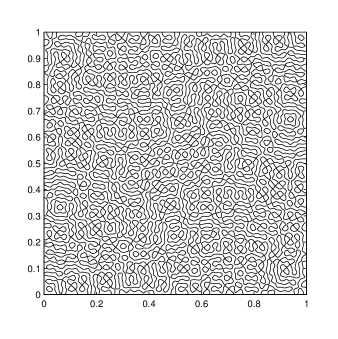
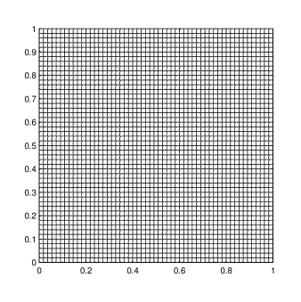
Fig. 4: The nodal lines of a Dirichlet eigenfunction $u(x_{1},x_{2})$ on the unit square, with the associated eigenvalue $\lambda=5525\pi^{2}$ of multiplicity 12. The eigenfunction was obtained as a linear combination of terms $\sin(\pi n_{1}x_{1})\sin(\pi n_{2}x_{2})$, with $n_{1}^{2}+n_{2}^{2}=5525$ and randomly chosen coefficients. For comparison, another eigenfunction with the same eigenvalue, $\sin(50\pi x_{1})\sin(55\pi x_{2})$, is shown.

Pleijel sharpened the Courant’s theorem by showing that the upper bound $m$ for the number $\nu_{m}$ of nodal domains is attained only for a finite number of eigenfunctions [399]. Moreover, he obtained the upper limit: $\varlimsup\limits_{m\to\infty}\nu_{m}/m=4/j_{0,1}^{2}\approx 0.691...$. Note that Lewy constructed spherical harmonics of any degree $n$ whose nodal sets have one component for odd $n$ and two components for even $n$ implying that no non-trivial lower bound for $\nu_{m}$ is possible [321]. We also mention that the counting of nodal domains can be viewed as partitioning of the domain into a fixed number of subdomains and minimizing an appropriate “energy” of the partition (e.g., the maximum of the ground state energies of the subdomains). When a partition corresponds to an eigenfunction, the ground state energies of all the nodal domains are the same, i.e., it is an equipartition [60].

Blum et al. considered the distribution of the (properly normalized) number of nodal domains of the Dirichlet-Laplacian eigenfunctions in 2D quantum billiards and showed the existence of the limiting distribution in the high-frequency limit (i.e., when $\lambda_{m}\to\infty$) [76]. These distributions were argued to be universal for systems with integrable or chaotic classical dynamics that allows one to distinguish them and thus provides a new criterion for quantum chaos (see Sec. 7.7.4). It was also conjectured that the distribution of nodal domains for chaotic systems coincides with that for Gaussian random functions.

Bogomolny and Schmit proposed a percolation-like model to describe the nodal domains which permitted to perform analytical calculations and agreed well with numerical simulations [77]. This model allows one to apply ideas and methods developed within the percolation theory [472] to the field of quantum chaos. Using the analogy with Gaussian random functions, Bogomolny and Schmit obtained that the mean and variance of the number $\nu_{m}$ of nodal domains grow as $m$, with explicit formulas for the prefactors. From the percolation theory, the distribution of the area $s$ of the connected nodal domains was conjectured to follow a power law, $n(s)\propto s^{-187/91}$, as confirmed by simulations [77]. In the particular case of random Gaussian spherical harmonics, Nazarov and Sodin rigorously derived the asymptotic behavior for the number $\nu_{n}$ of nodal domains of the harmonic of degree $n$ [367]. They proved that as $n$ grows to infinity, the mean of $\nu_{n}/n^{2}$ tends to a positive constant, and that $\nu_{n}/n^{2}$ exponentially concentrates around this constant (we recall that the associate eigenvalue is $n(n+1)$).

The geometrical structure of nodal lines and domains has been intensively studied (see [366, 400] for further discussion of the asymptotic nodal geometry). For instance, the length of the nodal line of an eigenfunction of the Laplace operator in two-dimensional Riemannian manifolds was separately investigated by Brüning, Yao and Nadirashvili who obtained its lower and upper bounds [90, 507, 362]. In addition, a number of conjectures about the properties of particular eigenfunctions were discussed in the literature. We mention three of them:

(i) In 1967, Payne conjectured that the second Dirichlet eigenfunction $u_{2}$ cannot have a closed nodal line in a bounded planar domain [390, 394]. This conjecture was proved for convex domains [5, 353] and disproved by non-convex domains [245], see also [256, 216].

(ii) The hot spots conjecture formulated by J. Rauch in 1974 says that the maximum of the second Neumann eigenfunction is attained at a boundary point. This conjecture was proved by Banuelos and Burdzy for a class of planar domains [41] but in general the statement is wrong, as shown by several counter-examples [102, 257, 54, 104].

(iii) Liboff formulated several conjectures; one of them states that the nodal surface of the first-excited state of a 3D convex domain intersects its boundary in a single simple closed curve [323].

The analysis of nodal lines that describe zeros of eigenfunctions, can be extended to other level sets. For instance, a level set of the first Dirichlet eigenfunction $u_{1}$ on a bounded convex domain $\Omega\in{\mathbb{R}}^{d}$ is itself convex [274]. Grieser and Jerison estimated the size of the first eigenfunction uniformly for all convex domains [217]. In particular, they located the place where $u_{1}$ achieves its maximum to within a distance comparable to the inradius, uniformly for arbitrarily large diameter. Other geometrical characteristics (e.g., the volume of a set on which an eigenfunction is positive) can also be analyzed [364].

6 Estimates for Laplacian eigenfunctions

The “amplitudes” of eigenfunctions can be characterized either globally by their $L_{p}$ norms

$$\|u\|_{p}\equiv\left(\int\limits_{\Omega}dx~{}|u(x)|^{p}\right)^{1/p}\qquad(p\geq 1),$$ (58)

or locally by pointwise estimates. Since eigenfunctions are defined up to a multiplicative constant, one often uses $L_{2}(\Omega)$ normalization: $\|u\|_{2}=1$. Note also the limiting case of $L_{\infty}$-norm

$$\|u\|_{\infty}\equiv\operatorname{ess\,sup}\limits_{x\in\Omega}|u(x)|=\max\limits_{x\in\Omega}|u(x)|$$ (59)

(the first equality is the general definition, while the second equality is applicable for eigenfunctions). It is worth recalling Hölder’s inequality for any two measurable functions $u$ and $v$ and for any positive $p$, $q$ such that $1/p+1/q=1$:

$$\|uv\|_{1}\leq\|u\|_{p}\|v\|_{q}.$$ (60)

For a bounded domain $\Omega\subset{\mathbb{R}}^{d}$ (with a finite Lebesgue measure $\mu_{d}(\Omega)$), Hölder’s inequality implies

$$\|u\|_{p}\leq[\mu_{d}(\Omega)]^{\frac{1}{p}-\frac{1}{p^{\prime}}}\|u\|_{p^{\prime}}\qquad(1\leq p\leq p^{\prime}).$$ (61)

We also mention Minkowski’s inequality for two measurable functions and any $p\geq 1$:

$$\|u+v\|_{p}\leq\|u\|_{p}+\|v\|_{p}.$$ (62)

6.1 First (ground) Dirichlet eigenfunction

The Dirichlet eigenfunction $u_{1}$ associated with the first eigenvalue $\lambda_{1}>0$ does not change the sign in $\Omega$ and may be taken to be positive. It satisfies the following inequalities.

(i) Payne and Rayner showed in two dimensions that

$$\|u_{1}\|_{2}\leq\frac{\sqrt{\lambda_{1}}}{\sqrt{4\pi}}~{}\|u_{1}\|_{1},$$ (63)

with equality if and only if $\Omega$ is a disk [391, 392]. Kohler-Jobin gave an extension of this inequality to higher dimensions [283] (see [392, 284, 132] for other extensions):

$$\|u_{1}\|_{2}\leq\frac{\lambda_{1}^{d/4}}{\sqrt{2d\omega_{d}[j_{\frac{d}{2}-1,1}]^{d-2}}}~{}\|u_{1}\|_{1}.$$ (64)

(ii) Payne and Stakgold derived two inequalities for a convex domain in 2D

$$\frac{\pi}{2\mu_{2}(\Omega)}\|u_{1}\|_{1}\leq\|u_{1}\|_{\infty}$$ (65)

and

$$u_{1}(x)\leq|x-{\partial\Omega}|\frac{\sqrt{\lambda_{1}}}{\mu_{2}(\Omega)}\|u_{1}\|_{1}\qquad(x\in\Omega),$$ (66)

where $|x-{\partial\Omega}|$ is the distance from a point $x$ in $\Omega$ to the boundary ${\partial\Omega}$ [393].

(iii) van den Berg proved the following inequality for $L_{2}$-normalized eigenfunction $u_{1}$ when $\Omega$ is an open, bounded and connected set in ${\mathbb{R}}^{d}$ ($d=2,3,\dots$):

$$\|u_{1}\|_{\infty}\leq\frac{2^{\frac{2-d}{2}}}{\pi^{d/4}\sqrt{\Gamma(d/2)}}~{}\frac{\left({j_{\frac{d-2}{2},1}}\right)^{\frac{d-2}{2}}}{|{J_{\frac{d}{2}}\bigl{(}j_{\frac{d-2}{2},1}\bigr{)}}|}~{}\rho^{-d/2},$$ (67)

with equality if and only if $\Omega$ is a ball, where $\rho$ is the inradius (Eq. (41)) [493]. van den Berg also conjectured the stronger inequality for an open bounded convex domain $\Omega\subset{\mathbb{R}}^{d}$:

$$\|u_{1}\|_{\infty}\leq C_{d}\rho^{-d/2}(\rho/\delta)^{1/6},$$ (68)

where $\delta$ is the diameter of $\Omega$, and $C_{d}$ is a universal constant independent of $\Omega$.

(iv) Kröger obtained another upper bound for $\|u_{1}\|_{\infty}$ for a convex domain $\Omega\subset{\mathbb{R}}^{d}$. Suppose that $\lambda_{1}(D)\geq\Lambda(\delta)$ for every convex subdomain $D\subset\Omega$ with $\mu_{d}(D)\leq\delta\mu_{d}(\Omega)$ and positive numbers $\delta$ and $\Lambda(\delta)$. The first eigenfunction $u_{1}$ which is normalized such that $\|u_{1}\|_{2}^{2}=\mu_{d}(\Omega)$, satisfies

$$\|u_{1}\|_{\infty}\leq C_{d}\delta^{-1/2}\bigl{[}1+\ln\|u_{1}\|_{\infty}-\ln(1-\lambda_{1}/\Lambda(\delta))\bigr{]}^{d/2},$$ (69)

with a universal positive constant $C_{d}$ which depends only on the dimension $d$ [293].

(v) Pang investigated how the first Dirichlet eigenvalue and eigenfunction would change when the domain slightly shrinks [383, 384]. For a bounded simply connected open set $\Omega\subset{\mathbb{R}}^{2}$, let

$$\Omega_{\epsilon}\supseteq\left\{x\in\Omega:|x-{\partial\Omega}|\geq\epsilon\right\}$$

be its interior, i.e., $\Omega$ without an $\epsilon$ boundary layer. Let $\lambda_{m}^{\epsilon}$ and $u_{m}^{\epsilon}$ be the Dirichlet eigenvalues and $L_{2}$-normalized eigenfunctions in $\Omega_{\epsilon}$ (with $\lambda_{m}^{0}=\lambda_{m}$ and $u_{m}^{0}=u_{m}$ referring to the original domain $\Omega$). Then, for all $\epsilon\in(0,\rho/2)$,

$$\begin{split}|\lambda_{1}^{\epsilon}-\lambda_{1}|&\leq C_{1}\epsilon^{1/2},\\ \|u_{1}-T_{\epsilon}u_{1}^{\epsilon}\|_{L_{\infty}(\Omega)}&\leq\left[{C_{2}+C_{3}(\lambda_{2}-\lambda_{1})^{-1/2}+C_{4}(\lambda_{2}-\lambda_{1})^{-1}}\right]\epsilon^{1/2},\\ \end{split}$$ (70)

where $\rho$ is the inradius of $\Omega$ (Eq. (41)), $T_{\epsilon}$ is the extension operator from $\Omega_{\epsilon}$ to $\Omega$, and

$$C_{1} = \rho^{-3/2}\beta^{9/4}~{}\frac{2^{9}\gamma_{1}^{4}}{3\pi^{9/4}},\qquad C_{2}=\rho^{-3/2}\beta^{13/4}~{}\frac{2^{12}\gamma_{1}^{5}}{\pi^{15/4}},$$

$$C_{3} = \rho^{-5/2}\beta^{4}\biggl{(}\frac{2^{15}\gamma_{1}^{6}\gamma_{2}}{3\sqrt{2\alpha}\pi^{9/2}}\biggr{)}\biggl{[}1+\frac{9\gamma_{1}}{\pi^{3/4}}\beta^{3/4}\biggr{]},$$

$$C_{4} = \rho^{-7/2}\beta^{7}\biggl{(}\frac{2^{26}\gamma_{1}^{10}\gamma_{2}^{2}}{81\sqrt{2}~{}\alpha~{}\pi^{15/2}}\biggr{)}\biggl{[}1+18\gamma_{1}\beta^{3/4}+\frac{81\gamma_{1}^{2}}{\pi^{3/2}}\beta^{3/2}\biggr{]},$$

where $\beta=\mu_{2}(\Omega)/\rho^{2}$, $\alpha$ is the constant from Eq. (40) (for which one can use the best known estimate $\alpha=0.6197...$ from [39]), and $\gamma_{1}$ and $\gamma_{2}$ are the first and second Dirichlet eigenvalues for the unit disk: $\gamma_{1}=j_{0,1}^{2}\approx 5.7832$ and $\gamma_{2}=j_{1,1}^{2}\approx 14.6820$. Moreover, when $\Omega$ is the cardioid in ${\mathbb{R}}^{2}$, the term $\epsilon^{1/2}$ cannot be improved.

In addition, Davies proved that for a bounded simply connected open set $\Omega\in{\mathbb{R}}^{2}$ and for any $\beta\in(0,1/2)$, there exists $c_{\beta}\geq 1$ such that [149]

$$|\lambda_{1}^{\epsilon}-\lambda_{1}|\leq c_{\beta}\epsilon^{\beta}$$ (71)

for all sufficiently small $\epsilon>0$. The estimate also holds for higher Dirichlet eigenvalues.

6.2 Estimates applicable for all eigenfunctions

6.2.1 Estimates through the Green function

Using the spectral decomposition (9) of the Green function $G(x,y)$, one can rewrite Eq. (1) as

$$u_{m}(x)=\lambda_{m}\int\limits_{\Omega}G(x,y)u_{m}(y)dy,$$

from which Hölder inequality (60) yields a family of simple pointwise estimates

$$|u_{m}(x)|\leq\lambda_{m}\|u_{m}\|_{\frac{p}{p-1}}\left(\int\limits_{\Omega}|G(x,y)|^{p}dy\right)^{1/p},$$ (72)

with any $p\geq 1$. Here, a single function of $x$ in the right-hand side bounds all the eigenfunctions. In particular, for $p=1$, one gets

$$|u_{m}(x)|\leq\lambda_{m}\|u_{m}\|_{\infty}\int\limits_{\Omega}|G(x,y)|dy.$$ (73)

For Dirichlet boundary condition, $G(x,y)$ is positive everywhere in $\Omega$ so that

$$|u_{m}(x)|\leq\lambda_{m}\|u_{m}\|_{\infty}~{}U(x),\qquad U(x)=\int\limits_{\Omega}G(x,y)dy,$$ (74)

where $U(x)$ solves the boundary value problem

$$-\Delta U(x)=1\quad(x\in\Omega),\qquad U(x)=0\quad(x\in{\partial\Omega}).$$ (75)

The solution of this equation is known to be the mean first passage time to the boundary ${\partial\Omega}$ from an interior point $x$ [420]. The inequalities (73, 74) (or their extensions) were reported by Moler and Payne [360] (Sect. 6.2.2) and were used by Filoche and Mayboroda for determining the geometrical structure of eigenfunctions [186] (Sect. 6.2.6). Note that the function $U(x)$ was also considered by Gorelick et al. for a reliable extraction of various shape properties of a silhouette, including part structure and rough skeleton, local orientation and aspect ratio of different parts, and convex and concave sections of the boundaries [209].

6.2.2 Bounds for eigenvalues and eigenfunctions of symmetric operators

Moler and Payne derived simple bounds for eigenvalues and eigenfunctions of symmetric operators by considering their extensions [360]. As a typical example, one can think of the Dirichlet-Laplace operator in a bounded domain $\Omega$ (symmetric operator $A$) and of the Laplace operator without boundary conditions (extension $A_{*}$). An approximation to an eigenvalue and eigenfunction of $A$ can be obtained by solving a simpler eigenvalue problem $A_{*}u_{*}=\lambda_{*}u_{*}$ without boundary condition. If there exists a function $w$ such that $A_{*}w=0$ and $w=u_{*}$ at the boundary of $\Omega$ and if $\displaystyle\varepsilon=\frac{\|w\|_{L_{2}(\Omega)}}{\|u_{*}\|_{L_{2}(\Omega)}}<1$, then there exists an eigenvalue $\lambda_{k}$ of $A$ satisfying

$$\frac{|\lambda_{*}|}{1+\varepsilon}\leq|\lambda_{k}|\leq\frac{|\lambda_{*}|}{1-\varepsilon}.$$ (76)

Moreover, if $\|u_{*}\|_{L_{2}(\Omega)}=1$ and $u_{k}$ is the $L_{2}$-normalized projection of $u_{*}$ onto the eigenspace of $\lambda_{k}$, then

$$\|u_{*}-u_{k}\|_{L_{2}(\Omega)}\leq\frac{\varepsilon}{\alpha}\left(1+\frac{\varepsilon^{2}}{\alpha^{2}}\right)^{1/2},\qquad{\rm with}\quad\alpha=\min\limits_{\lambda_{n}\neq\lambda_{k}}\frac{|\lambda_{n}-\lambda_{*}|}{|\lambda_{n}|}.$$ (77)

If $u_{*}$ is a good approximation to an eigenfunction of the Dirichlet-Laplace operator, then it must be close to zero on the boundary of $\Omega$, yielding small $\varepsilon$ and thus accurate lower and upper bounds in (76). The accuracy of the bound (77) also depends on the separation $\alpha$ between eigenvalues.

In the same work, Moler and Payne also provided pointwise bounds for eigenfunctions that rely on Green’s functions (an extension of Sec. 6.2.1).

6.2.3 Estimates for $L_{p}$-norms

Chiti extended Payne-Rayner’s inequality (63) to the eigenfunctions of linear elliptic second order operators in divergent form, with Dirichlet boundary condition [132]. For the Laplace operator in a bounded domain $\Omega\subset{\mathbb{R}}^{d}$, Chiti’s inequality for any real numbers $q\geq p>0$ states:

$$\|u\|_{q}\leq\|u\|_{p}~{}(d\omega_{d})^{\frac{1}{q}-\frac{1}{p}}\lambda^{\frac{q-p}{2pq}d}\frac{\biggl{(}\int\limits_{0}^{j_{\frac{d}{2}-1,1}}dr~{}r^{d-1+q(1-d/2)}[J_{\frac{d}{2}-1}(r)]^{q}\biggr{)}^{1/q}}{\biggl{(}\int\limits_{0}^{j_{\frac{d}{2}-1,1}}dr~{}r^{d-1+p(1-d/2)}[J_{\frac{d}{2}-1}(r)]^{p}\biggr{)}^{1/p}},$$ (78)

where $\omega_{d}$ is given by Eq. (32).

6.2.4 Pointwise bounds for Dirichlet eigenfunctions

Banuelos derived a pointwise upper bound for $L_{2}$-normalized Dirichlet eigenfunctions [40]

$$|u_{m}(x)|\leq\lambda_{m}^{d/4}\qquad(x\in\Omega).$$ (79)

van den Berg and Bolthausen proved several estimates for $L_{2}$-normalized Dirichlet eigenfunctions [491]. Let $\Omega\subset{\mathbb{R}}^{d}$ $(d=2,3,\dots)$ be an open bounded domain with boundary ${\partial\Omega}$ which satisfies an $\alpha$-uniform capacitary density condition with some $\alpha\in(0,1]$, i.e.

$$\textrm{Cap}\{{\partial\Omega}\cap B(x;r)\}\geq\alpha\textrm{Cap}\{B(x;r)\},\quad x\in{\partial\Omega},~{}0<r<\delta,$$ (80)

where $B(x,r)$ is the ball of radius $r$ centered at $x$, $\delta$ is the diameter of $\Omega$ (Eq. (50)), and Cap is the logarithmic capacity for $d=2$ and the Newtonian (or harmonic) capacity for $d>2$ (the harmonic capacity of an Euclidean domain presents a measure of its “size” through the total charge the domain can hold at a given potential energy [161]). The condition (80) guarantees that all points of ${\partial\Omega}$ are regular. The following estimates hold

(i) in two dimensions ($d=2$), for all $m=1,2,\dots$ and all $x\in\Omega$ such that $|x-{\partial\Omega}|\sqrt{\lambda_{m}}<1$, one has

$$|u_{m}(x)|\leq\left\{\frac{6\lambda_{m}\ln(\alpha^{2\pi}/2)}{\ln{\left({|x-{\partial\Omega}|\sqrt{\lambda_{m}}}\right)}}\right\}^{1/2}.$$ (81)

(ii) in higher dimensions ($d>2$), for all $m=1,2,\dots$ and all $x\in\Omega$ such that

$$|x-{\partial\Omega}|\sqrt{\lambda_{m}}\leq\left({\frac{\alpha^{6}}{2^{13}}}\right)^{1+\gamma(d-1)/(d-2)},$$ (82)

with $\displaystyle\gamma=\frac{3^{-d-1}\alpha}{\ln(2(2/\alpha)^{1/(d-2)})}$, one has

$$|u_{m}(x)|\leq 2\lambda_{m}^{d/4}\biggl{(}|x-{\partial\Omega}|\sqrt{\lambda_{m}}\biggr{)}^{\frac{1}{2}((1/\gamma)+(d-1)/(d-2))^{-1}}.$$ (83)

(iii) for a planar simply connected domain and all $m=1,2,\dots$,

$$|u_{m}(x)|\leq m~{}2^{9/2}\pi^{1/4}\frac{(\mu_{2}(\Omega))^{1/4}}{\rho^{2}}~{}|x-{\partial\Omega}|^{1/2}\qquad(x\in\Omega),$$ (84)

where $\rho$ is the inradius of $\Omega$ (see Eq. (41)), and the inequality is sharp.

6.2.5 Upper and lower bounds for normal derivatives of Dirichlet eigenfunctions

Suppose that $M$ is a compact Riemannian manifold with boundary and $u$ is an $L_{2}$-normalized Dirichlet eigenfunction with eigenvalue $\lambda$. Let $\psi$ be its normal derivative at the boundary. A scaling argument suggests that the $L_{2}$-norm of $\psi$ will grow as $\sqrt{\lambda}$ as $\lambda\to\infty$. Hassell and Tao proved that

$$c_{M}\sqrt{\lambda}\leq\|\psi\|_{L_{2}(\partial M)}\leq C_{M}\sqrt{\lambda},$$ (85)

where the upper bound holds for any Riemannian manifold, while the lower bound is valid provided that $M$ has no trapped geodesics [228]. The positive constants $c_{M}$ and $C_{M}$ depend on $M$, but not on $\lambda$.

6.2.6 Estimates for restriction onto a subdomain

For a bounded domain $\Omega\subset{\mathbb{R}}^{d}$, Filoche and Mayboroda obtained the upper bound for the $L_{2}$-norm of a Dirichlet-Laplacian eigenfunction $u$ associated to $\lambda$, in any open subset $D\subset\Omega$ [186]:

$$\|u\|_{L_{2}(D)}\leq\left(1+\frac{\lambda}{d_{D}(\lambda)}\right)\|v\|_{L_{2}(D)},$$ (86)

where the function $v$ solves the boundary value problem in $D$:

$$\Delta v=0\quad(x\in D),\qquad v=u\quad(x\in{\partial D}).$$

and $d_{D}(\lambda)$ is the distance from $\lambda$ to the spectrum of the Dirichlet-Laplace operator in $D$. Note also that the above bound was proved for general self-adjoint elliptic operators [186]. When combined with Eq. (74), this inequality helps one investigate the spatial distribution of eigenfunctions because harmonic functions are in general much easier to analyze or estimate than eigenfunctions.

We complete the above estimate by a lower bound [371]

$$\|u\|_{L_{2}(D)}\geq\frac{\lambda_{1}(D)}{\lambda+\lambda_{1}(D)}\|v\|_{L_{2}(D)},$$ (87)

where $\lambda_{1}(D)$ is the first Dirichlet eigenvalue of the subdomain $D$.

7 Localization of eigenfunctions

“Localization” is defined in the Webster’s dictionary as “act of localizing, or state of being localized”. The notion of localization appears in various fields of science and often has different meanings. Throughout this review, a function $u$ defined on a domain $\Omega\subset{\mathbb{R}}^{d}$, is called $L_{p}$-localized (for $p\geq 1$) if there exists a bounded subset $\Omega_{0}\subset\Omega$ which supports almost all $L_{p}$-norm of $u$, i.e.

$$\frac{\|u\|_{L_{p}(\Omega\setminus\Omega_{0})}}{\|u\|_{L_{p}(\Omega)}}\ll 1\qquad\textrm{and}\qquad\frac{\mu_{d}(\Omega_{0})}{\mu_{d}(\Omega)}\ll 1.$$ (88)

Qualitatively, a localized function essentially “lives” on a small subset of the domain and takes small values on the remaining part. For instance, a Gaussian function $\exp(-x^{2})$ on $\Omega={\mathbb{R}}$ is $L_{p}$-localized for any $p\geq 1$ since one can choose $\Omega_{0}=[-a,a]$ with large enough $a$ so that the ratio of $L_{p}$-norms can be made arbitrarily small, while the ratio of lengths $\mu_{1}(\Omega_{0})/\mu_{1}(\Omega)$ is strictly $0$. In turn, when $\Omega=[-A,A]$, the localization character of $\exp(-x^{2})$ on $\Omega$ becomes dependent on $A$ and thus conventional. A simple calculation shows that both ratios in (88) cannot be simultaneously made smaller than $1/(A+1)$ for any $p\geq 1$. For instance, if $A=3$ and the “threshold” 1/4 is viewed small enough, then we are justified to call $\exp(-x^{2})$ localized on $[-A,A]$. This example illustrates that the above inequalities do not provide a universal quantitative criterion to distinguish localized from non-localized (or extended) functions. In this section, we will describe various kinds of localization for which some quantitative criteria can be formulated. We will also show that the choice of the norm (i.e., $p$) may be important.

Another “definition” of localization was given by Felix et al. who combined $L_{2}$ and $L_{4}$ norms to define the “existence area” as [175]

$$S(u)=\frac{\|u\|_{L_{2}(\Omega)}^{4}}{\|u\|_{L_{4}(\Omega)}^{4}}.$$ (89)

A function $u$ was called localized when its existence area $S(u)$ was much smaller than the area $\mu_{2}(\Omega)$ [175] (this definition trivially extends to other dimensions). In fact, if a function is small in a subdomain, the fourth power diminishes it stronger than the second power. For instance, if $\Omega=(0,1)$ and $u$ is $1$ on the subinterval $\Omega_{0}=(1/4,1/2)$ and $0$ otherwise, one has $\|u\|_{L_{2}(\Omega)}=1/2$ and $\|u\|_{L_{4}(\Omega)}=1/\sqrt{2}$ so that $S(u)=1/4$, i.e., the length of the subinterval $\Omega_{0}$. This definition is still qualitative: e.g., in the above example, is the ratio $S(u)/\mu_{1}(\Omega)=1/4$ small enough to call $u$ localized? Note that a whole family of “existence areas” can be constructed by comparing $L_{p}$ and $L_{q}$ norms (with $p<q$),

$$S_{p,q}(u)=\left(\frac{\|u\|_{L_{p}(\Omega)}}{\|u\|_{L_{q}(\Omega)}}\right)^{\frac{1}{\frac{1}{p}-\frac{1}{q}}}.$$ (90)

7.1 Bound quantum states in a potential

The notion of bound, trapped or localized quantum states is known for a long time [421, 74]. The simplest “canonical” example is the quantum harmonic oscillator, i.e., a particle of mass $m$ in a harmonic potential of frequency $\omega$ which is described by the Hamiltonian

$$H=\frac{\hat{p}^{2}}{2m}+\frac{m\omega^{2}}{2}\hat{x}^{2}=-\frac{\hbar^{2}}{2m}\partial_{x}^{2}+\frac{m\omega^{2}}{2}x^{2},$$ (91)

where $\hat{p}=-i\hbar\partial_{x}$ is the momentum operator, and $\hat{x}=x$ is the position operator ($\hbar$ being the Planck’s constant). The eigenfunctions of this operator are well known:

$$\psi_{n}(x)=\sqrt{\frac{1}{2^{n}~{}n!}}\left(\frac{m\omega}{\pi\hbar}\right)^{1/4}\exp\left(-\frac{m\omega x^{2}}{2\hbar}\right)H_{n}\bigl{(}\sqrt{m\omega/\hbar}x\bigr{)},$$ (92)

where $H_{n}(x)$ are the Hermite polynomials. All these functions are localized in a region around the minimum of the harmonic potential (here, $x=0$), and rapidly decay outside this region. For this example, the definition (88) of localization is rigorous. In physical terms, the presence of a strong potential forbids the particle to travel far from the origin, the size of the localization region being $\sqrt{\hbar/(m\omega)}$. This so-called strong localization has been thoroughly investigated in physics and mathematics [337, 338, 3, 421, 460, 449, 453, 379].

7.2 Anderson localization

The previous example of a single quantum harmonic well is too idealized. A piece of matter contains an extremely large number of interacting atoms. Even if one focuses onto a single atom in an effective potential, the form of this potential may be so complicated that the study of the underlying eigenfunctions would in general be intractable. In 1958, Anderson considered a lattice model for a charge carrier in a random potential and proved the localization of eigenfunctions under certain conditions [9]. The localization of charge carriers means no electric current through the medium (insulating state), in contrast to metallic or conducting state when the charge carriers are not localized. The Anderson transition between insulating and conducting states is illustrated for the tight-binding model on Fig. 5. The shown eigenfunctions were computed by Obuse for three disorder strengths $W$ that correspond to metallic ($W<W_{0}$), critical ($W=W_{0}$), and insulating ($W>W_{0}$) states, $W_{0}=5.952$ being the critical disorder strength. The latter eigenfunction is strongly localized that prohibits diffusion of charge carriers (i.e., no electric current). The Anderson localization which explains the metal-insulator transitions in semiconductors, was thoroughly investigated during the last fifty years (see [482, 316, 291, 56, 428, 357, 170, 476, 475] for details and references). Similar localization phenomena were observed for microwaves with two-dimensional random scattering [142], for light in a disordered medium [504] and in disordered photonic crystals [452, 441], for matter waves in a controlled disorder [70] and in non-interacting Bose-Einstein condensate [429], and for ultrasound [248]. The multifractal structure of the eigenfunctions at the critical point (illustrated by Fig. 5b) has also been intensively investigated (see [170, 220] and references therein). Localization of eigenstates and transport phenomena in one-dimensional disordered systems are reviewed in [251]. An introduction to wave scattering and the related localization is given in [455].

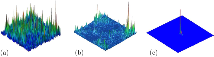
Fig. 5: Illustration of the Anderson transition in a tight-binding model (or so-called SU(2) model) in the two-dimensional symplectic class [20, 21, 372, 373]. Three shown eigenfunctions (with the energy close to $1$) were computed for three disorder strengths $W$ that correspond to (a) metallic state ($W<W_{0}$), (b) critical state ($W=W_{0}$), and (c) insulating state ($W>W_{0}$), $W_{0}=5.952$ being the critical disorder strength. The latter eigenfunction is strongly localized that prohibits diffusion of charge carriers (i.e., no electric current). The eigenfunctions were computed and provided by H. Obuse (unpublished earlier).

7.3 Trapping in infinite waveguides

In both previous cases, localization of eigenfunctions was related to an external potential. In particular, if the potential was not strong enough, Anderson localization could disappear (Fig. 5a). Is the presence of a potential necessary for localization? The formal answer is positive because the eigenstates of the Laplace operator in the whole space ${\mathbb{R}}^{d}$ are simply $e^{i(k\cdot x)}$ (parameterized by the vector $k$) which are all extended in ${\mathbb{R}}^{d}$. These waves are called “resonances” (not eigenfunctions) of the Laplace operator, as their $L_{2}$-norm is infinite.

The situation is different for the Laplace operator in a bounded domain with Dirichlet boundary condition. In quantum mechanics, such a boundary presents a “hard wall” that separates the interior of the domain with zero potential from the exterior of the domain with infinite potential. For instance, this “model” was employed by Crommie et al. to describe the confinement of electrons to quantum corrals on a metallic surface [140] (see also their figure 2 that shows the experimental spatial structure of the electron’s wavefunction). Although the physical interpretation of a boundary through an infinite potential is instructive, we will use the mathematical terminology and speak about the eigenvalue problem for the Laplace operator in a bounded domain without potential.

For unbounded domains, the spectrum of the Laplace operator consists of two parts: (i) the discrete (or point-like) spectrum, with eigenfunctions of finite $L_{2}$ norm that are necessarily “trapped” or “localized” in a bounded region of the waveguide, and (ii) the continuous spectrum, with associated functions of infinite $L_{2}$ norm that are extended over the whole domain. The continuous spectrum may also contain embedded eigenvalues whose eigenfunctions have finite $L_{2}$ norm. A wave excited at the frequency of the trapped eigenmode remains in the localization region and does not propagate. In this case, the definition (88) of localization is again rigorous, as for any bounded subset $\Omega_{0}$ of an unbounded domain $\Omega$, one has $\mu_{d}(\Omega_{0})/\mu_{d}(\Omega)=0$, while the ratio of $L_{2}$ norms can be made arbitrarily small by expanding $\Omega_{0}$.

This kind of localization in classical and quantum waveguides has been thoroughly investigated (see reviews [163, 328] and also references in [376]). In the seminal paper, Rellich proved the existence of a localized eigenfunction in a deformed infinite cylinder [422]. His results were significantly extended by Jones [264]. Ursell reported on the existence of trapped modes in surface water waves in channels [487, 488, 489], while Parker observed experimentally the trapped modes in locally perturbed acoustic waveguides [385, 386]. Exner and Seba considered an infinite bent strip of smooth curvature and showed the existence of trapped modes by reducing the problem to Schrödinger operator in the straight strip, with the potential depending on the curvature [171]. Goldstone and Jaffe gave the variational proof that the wave equation subject to Dirichlet boundary condition always has a localized eigenmode in an infinite tube of constant cross-section in any dimension, provided that the tube is not exactly straight [206]. This result was further extended by Chenaud et al. to arbitrary dimension [127]. The problem of localization in acoustic waveguides with Neumann boundary condition has also been investigated [167, 168]. For instance, Evans et al. considered a straight strip with an inclusion of arbitrary (but symmetric) shape [168] (see [150] for further extensions). Such an inclusion obstructed the propagation of waves and was shown to result in trapped modes. The effect of mixed Dirichlet, Neumann and Robin boundary conditions on the localization was also investigated (see [376, 97, 157, 191] and references therein). A mathematical analysis of guided water waves was developed by Bonnet-Ben Dhia and Joly [82] (see also [83]). Lower bounds for the eigenvalues below the cut-off frequency (for which the associated eigenfunctions are localized) were obtained by Ashbaugh and Exner for infinite thin tubes in two and three dimensions [22]. In addition, these authors derived an upper bound for the number of the trapped modes. Exner et al. considered the Laplacian in finite-length curved tubes of arbitrary cross-section, subject to Dirichlet boundary conditions on the cylindrical surface and Neumann conditions at the ends of the tube. They expressed a lower bound for the spectral threshold of the Laplacian through the lowest eigenvalue of the Dirichlet Laplacian in a torus determined by the geometry of the tube [173]. In a different work, Exner and co-worker investigated bound states and scattering in quantum waveguides coupled laterally through a boundary window [172].

Examples of waveguides with numerous localized states were reported in the literature. For instance, Avishai et al. demonstrated the existence of many localized states for a sharp “broken strip”, i.e., a waveguide made of two channels of equal width intersecting at a small angle $\theta$ [32]. Carini and co-workers reported an experimental confirmation of this prediction and its further extensions [116, 117, 331]. Bulgakov et al. considered two straight strips of the same width which cross at an angle $\theta\in(0,\pi/2)$ and showed that, for small $\theta$, the number of localized states is greater than $(1-2^{-2/3})^{3/2}/\theta$ [96]. Even for the simple case of two strips crossed at the right angle $\theta=\pi/2$, Schult et al. showed the existence of two localized states, one lying below the cut-off frequency and the other being embedded into the continuous spectrum [451].

7.4 Exponential estimate for eigenfunctions

Qualitatively, an eigenmode is trapped when it cannot “squeeze” outside the localization region through narrow channels or branches of the waveguide. This happens when typical spatial variations of the eigenmode, which are in the order of a wavelength $\pi\lambda^{-1/2}$, are larger than the size $a$ of the narrow part, i.e., $\pi\lambda^{-1/2}\geq a$ or $\lambda\leq\pi^{2}/a^{2}$ [253]. This simplistic argument suggests that there exists a threshold value $\mu$ (which may eventually be $0$), or so-called cut-off frequency, such that the eigenmodes with $\lambda\leq\mu$ are localized. Moreover, this qualitative geometrical interpretation is well adapted for both unbounded and bounded domains. While the former case of infinite waveguides was thoroughly investigated, the existence of trapped or localized eigenmodes in bounded domains has attracted less attention. Even the definition of localization in bounded domains remains conventional because all eigenfunctions have finite $L_{2}$ norm.

Fig. 6: Two examples of a bounded domain $\Omega=\Omega_{1}\cup\Omega_{2}$ with a branch of variable cross-sectional profile. When the eigenvalue $\lambda$ is smaller than the cut-off “frequency” $\mu$, the associated eigenfunction exponentially decays in the branch $\Omega_{2}$ and is thus mainly localized in $\Omega_{1}$. Note that the branch itself may even be increasing.

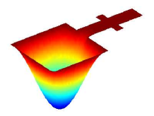
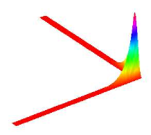
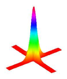
Fig. 7: Examples of localized Dirichlet Laplacian eigenfunctions with an exponential decay: square with a branch (from [151]), L-shape and crossing of two stripes (from [152]).

This problem was studied by Delitsyn and co-workers for domains with branches of variable cross-sectional profiles [151]. More precisely, one considers a bounded domain $\Omega\subset{\mathbb{R}}^{d}$ ($d=2,3,...$) with a piecewise smooth boundary ${\partial\Omega}$ and denote $Q(z)=\Omega\cap\{x\in{\mathbb{R}}^{d}~{}:~{}x_{1}=z\}$ the cross-section of $\Omega$ at $x_{1}=z\in{\mathbb{R}}$ by a hyperplane perpendicular to the coordinate axis $x_{1}$ (Fig. 6). Let

$$z_{1}=\inf\{z\in{\mathbb{R}}~{}:~{}Q(z)\neq\emptyset\},\qquad z_{2}=\sup\{z\in{\mathbb{R}}~{}:~{}Q(z)\neq\emptyset\},$$

and we fix some $z_{0}$ such that $z_{1}<z_{0}<z_{2}$. Let $\mu(z)$ be the first eigenvalue of the Laplace operator in $Q(z)$, with Dirichlet boundary condition on $\partial Q(z)$, and $\mu=\inf\limits_{z\in(z_{0},z_{2})}\mu(z)$. Let $u$ be a Dirichlet-Laplacian eigenfunction in $\Omega$, and $\lambda$ the associate eigenvalue. If $\lambda<\mu$, then

$$\|u\|_{L_{2}(Q(z))}\leq\|u\|_{L_{2}(Q(z_{0}))}\exp(-\beta\sqrt{\mu-\lambda}~{}(z-z_{0}))\quad(z\geq z_{0}),$$ (93)

with $\beta=1/\sqrt{2}$. Moreover, if $(e_{1}\cdot n(x))\geq 0$ for all $x\in{\partial\Omega}$ with $x_{1}>z_{0}$, where $e_{1}$ is the unit vector $(1,0,...,0)$ in the direction $x_{1}$, and $n(x)$ is the normal vector at $x\in{\partial\Omega}$ directed outwards the domain, then the above inequality holds with $\beta=1$.

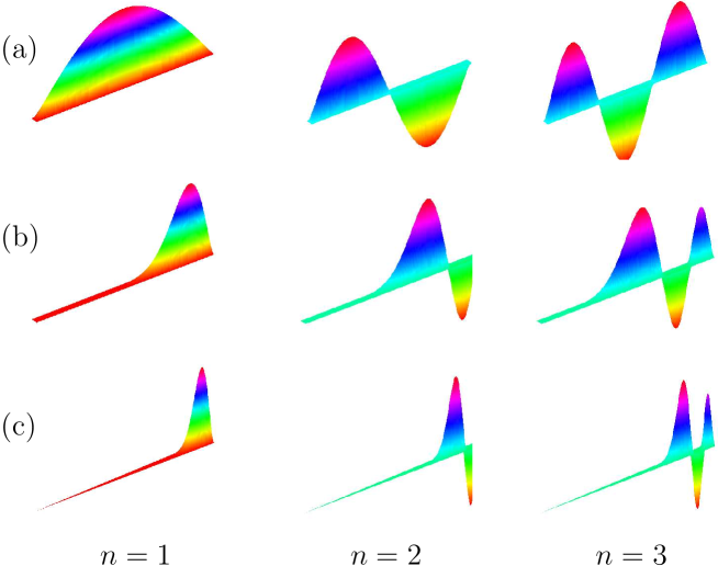
Fig. 8: The first three Dirichlet Laplacian eigenfunctions for three elongated domains: (a) rectangle of size $25\times 1$; (b) right trapezoid with bases $1$ and $0.9$ and height $25$ which is very close to the above rectangle; and (c) right triangle with edges $25$ and $1$ (half of the rectangle). There is no localization for the first shape, while the first eigenfunctions for the second and third domains tend to be localized.

In this statement, a domain $\Omega$ is arbitrarily split into two subdomains, $\Omega_{1}$ (with $x_{1}<z_{0}$) and $\Omega_{2}$ (with $x_{1}>z_{0}$), by the hyperplane at $x_{1}=z_{0}$ (the coordinate axis $x_{1}$ can be replaced by any straight line). Under the condition $\lambda<\mu$, the eigenfunction $u$ exponentially decays in the subdomain $\Omega_{2}$ which is loosely called “branch”. Note that the choice of the splitting hyperplane (i.e., $z_{0}$) determines the threshold $\mu$.

The theorem formalizes the notion of the cut-off frequency $\mu$ for branches of variable cross-sectional profiles and provides a constructive way for its computation. For instance, if $\Omega_{2}$ is a rectangular channel of width $a$, the first eigenvalue in all cross-sections $Q(z)$ is $\pi^{2}/a^{2}$ (independently of $z$) so that $\mu=\pi^{2}/a^{2}$, as expected. The exponential estimate quantifies the “difficulty” of penetration, or “squeezing”, into the branch $\Omega_{2}$ and ensures the localization of the eigenfunction $u$ in $\Omega_{1}$. Since the cut-off frequency $\mu$ is independent of the subdomain $\Omega_{1}$, one can impose any boundary condition on $\partial\Omega_{1}$ (that still ensures the self-adjointness of the Laplace operator). In turn, the Dirichlet boundary condition on the boundary of the branch $\Omega_{2}$ is relevant, although some extensions were discussed in [151]. It is worth noting that the theorem also applies to infinite branches $\Omega_{2}$, under supplementary condition $\mu(z)\to\infty$ to ensure the existence of the discrete spectrum.

According to this theorem, the $L_{2}$-norm of an eigenfunction with $\lambda<\mu$ in $\Omega(z)=\Omega\cap\{x\in{\mathbb{R}}^{d}~{}:~{}x_{1}>z\}$ can be made exponentially small provided that the branch $\Omega_{2}$ is long enough. Taking $\Omega_{0}=\Omega\setminus\Omega(z)$, the ratio of $L_{2}$-norms in Eq. (88) can be made arbitrarily small. However, the second ratio may not be necessarily small. In fact, its smallness depends on the shape of the domain $\Omega$. This is once again a manifestation of the conventional character of localization in bounded domains.

Figure 7 presents several examples of localized Dirichlet Laplacian eigenfunctions showing an exponential decay along the branches. Since an increase of branches diminishes the eigenvalue $\lambda$ and thus further enhances the localization, the area of the localized region $\Omega_{1}$ can be made arbitrarily small with respect to the total area (one can even consider infinite branches). Examples of an L-shape and a cross illustrate that the linear sizes of the localized region do not need to be large in comparison with the branch width (a sufficient condition for getting this kind of localization was proposed in [152]). It is worth noting that the separation into the localized region and branches is arbitrary. For instance, Fig. 8 shows several localized eigenfunctions for elongated triangle and trapezoid, for which there is no explicit separation.

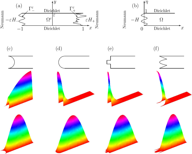
Fig. 9: (a) A thin cylinder $\Omega^{\varepsilon}\in{\mathbb{R}}^{2}$ of width $\varepsilon$ with two distorted ends defined by functions $H_{\pm}(\eta)$, $\eta\in\omega=(0,1)$. (b) In the limit $\varepsilon\to 0$, the analysis is reduced to a semi-infinite cylinder $\Omega$ with one distorted end. (c,d,e,f) Four semi-infinite cylinders with various distorted ends (top), the first eigenfunction for the Laplace operator in these shapes with mixed Dirichlet-Neumann boundary condition (middle), and the first eigenfunction for the Laplace operator with purely Dirichlet boundary condition. According to the sufficient conditions (94,95), the first eigenfunction is localized near the distorted end for cases ’d’, ’e’ and ’f’, and not localized for the case ’c’. No localization happens when the Dirichlet boundary condition is set over the whole domain. For numerical computation, semi-infinite cylinders were “truncated” and auxilary Dirichlet boundary condition was set at the right straight end.

Localization and exponential decay of Laplacian eigenfunctions were observed for various perturbations of cylindrical domains [272, 365, 115]. For instance, Kamotskii and Nazarov studied localization of eigenfunctions in a neighborhood of the lateral surface of a thin domain [272]. Nazarov and co-workers analyzed the behavior of eigenfunctions for thin cylinders with distorted ends [365, 115]. For a bounded domain $\omega\subset{\mathbb{R}}^{n-1}$ ($n\geq 2$) with a simple closed Lipschitz contour $\partial\omega$ and Lipschitz functions $H_{\pm}(\eta)$ in $\bar{\omega}=\omega\cup\partial\omega$, the thin cylinder with distorted ends is defined for a given small $\varepsilon>0$ as

$$\Omega^{\varepsilon}=\{(x,y)\in{\mathbb{R}}\times{\mathbb{R}}^{n-1}~{}:~{}y=\varepsilon\eta,~{}-1-\varepsilon H_{-}(\eta)<x<1+\varepsilon H_{+}(\eta),~{}\eta\in\omega\}.$$

One can view this domain as a thin cylinder $[-1,1]\times(\varepsilon\omega)$ to which two distorted “cups” characterized by functions $H_{\pm}$, are attached (Fig. 9a). The Neumann boundary condition is imposed on the curved ends $\Gamma^{\varepsilon}_{\pm}$:

$$\Gamma^{\varepsilon}_{\pm}=\{(x,y)\in{\mathbb{R}}\times{\mathbb{R}}^{n-1}~{}:~{}y=\varepsilon\eta,~{}x=\pm 1\pm\varepsilon H_{\pm}(\eta),~{}\eta\in\omega\},$$

while the Dirichlet boundary condition is set on the remaining lateral side of the domain: $\Sigma^{\varepsilon}=\partial\Omega^{\varepsilon}\backslash(\overline{\Gamma^{\varepsilon}_{+}\cup\Gamma^{\varepsilon}_{+}})$. When the ends of the cylinder are straight ($H_{\pm}\equiv 0$), the eigenfunctions are factored as $u_{mn}(x,y)=\cos(\pi m(x+1)/2)\varphi_{n}(y)$, where $\varphi_{n}(y)$ are the eigenfunctions of the Laplace operator in the cross-section $\omega$ with Dirichlet boundary condition. These eigenfunctions are extended over the whole cylinder, due to the cosine factor. Nazarov and co-workers showed that distortion of the ends (i.e., $H_{\pm}\neq 0$) may lead to localization of the ground eigenfunction in one (or both) ends, with an exponential decay toward the central part. In the limit $\varepsilon\to 0$, the thinning of the cylinder can be alternatively seen as its outstretching, allowing one to reduce the analysis to a semi-infinite cylinder with one distorted end (Fig. 9b), described by a single function $H(\eta)$:

$$\Omega=\{(x,\eta)\in{\mathbb{R}}\times{\mathbb{R}}^{n-1}~{}:~{}-H(\eta)<x,~{}\eta\in\omega\}.$$

Two sufficient conditions for getting the localized ground eigenfunction at the distorted end were proposed in [115]:

(i) For $H\in C(\bar{\omega})$, the sufficient condition reads

$$\int\limits_{\omega}d\eta~{}H(\eta)\biggl{(}|\nabla\varphi_{1}(\eta)|^{2}-\mu_{1}[\varphi_{1}(\eta)]^{2}\biggr{)}<0,$$ (94)

where $\mu_{1}$ is the smallest eigenvalue corresponding to $\varphi_{1}$ in the cross-section $\omega$ (in two dimensions, when $\omega=[-1/2,1/2]$, one has $\varphi_{1}(\eta)=\sin\pi(\eta+1/2)$ and $\mu_{1}=\pi^{2}$ so that this condition reads $\int_{-1/2}^{1/2}d\eta~{}H(\eta)\cos(2\pi\eta)>0$ [365]);

(ii) Under a stronger assumption $H\in C^{2}(\bar{\omega})$, the sufficient condition simplifies to

$$\int\limits_{\omega}d\eta~{}[\varphi_{1}(\eta)]^{2}\Delta H(\eta)<0.$$ (95)

This inequality becomes true for a subharmonic profile $-H$ (i.e., for $\Delta H(\eta)<0$) with but false for superharmonic.

Figure 9 shows several examples for which the sufficient condition is either satisfied (9d,e,f), or not (9c). Nazarov and co-workers showed that these results are applicable to bounded thin cylinders for small enough $\varepsilon$. In addition, they found out a domain where the first eigenfunction concentrates at the both ends simultaneously. Finally, they showed that no localization happens in the case in which the mixed Dirichlet-Neumann boundary condition is replaced by the Dirichlet boundary condition onto the whole boundary, as illustrated on Fig. 9 (see [115] for further discussions and results).

Friedlander and Solomyak studied the spectrum of the Dirichlet Laplacian in a family of narrow strips of variable profile: $\Omega=\{(x,y)\in{\mathbb{R}}^{2}~{}:~{}-a<x<b,~{}0<y<\varepsilon h(x)\}$ [195, 196]. The main assumption was that $x=0$ is the only point of global maximum of the positive, continuous function $h(x)$. In the limit $\varepsilon\to 0$, they found the two-term asymptotics of the eigenvalues and the one-term asymptotics of the corresponding eigenfunctions. The asymptotic formulas obtained involve the eigenvalues and eigenfunctions of an auxiliary ODE on ${\mathbb{R}}$ that depends only on the behavior of $h(x)$ as $x\to 0$, i.e., in the vicinity of the widest cross-section of the strip.

7.5 Dumbbell domains

Yet another type of localization emerges for domains that can be split into two or several subdomains with narrow connections (of “width” $\varepsilon$) [417], a standard example being a dumbbell: $\Omega^{\varepsilon}=\Omega_{1}\cup Q^{\varepsilon}\cup\Omega_{2}$ (Fig. 10a). The asymptotic behavior of eigenvalues and eigenfunctions in the limit $\varepsilon\to 0$ was thoroughly investigated for both Dirichlet and Neumann boundary conditions [261]. We start by considering Dirichlet boundary condition.

Fig. 10: (a) A dumbbell domain $\Omega^{\varepsilon}$ is the union of two bounded domains $\Omega_{1}$, $\Omega_{2}$ and a narrow “connector” $Q^{\varepsilon}$ of width $\varepsilon$. (b) In the limit $\varepsilon\to 0$, the connector degenerates to a curve (here, an interval) so that the subdomains $\Omega_{1}$ and $\Omega_{2}$ become disconnected. (c) In Beale’s work, $\Omega^{\varepsilon}$ is composed of two components, a bounded domain $\Omega_{1}$ and unbounded domain $\Omega_{2}$, which are connected by a narrow channel $Q^{\varepsilon}$.

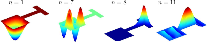
Fig. 11: Several Dirichlet Laplacian eigenfunctions for a dumbbell domain which is composed of two rectangles and connected by the third rectangle (from [151]). The 1st and 7th eigenfunctions are localized in the larger subdomain, the 8th eigenfunction is localized in the smaller subdomain, while the 11th eigenfunction is not localized at all. Note that the width of connection is not small ($1/4$ of the width of both subdomains).

In the limiting case of zero width connections, the subdomains $\Omega_{i}$ ($i=1,...,N$) become disconnected, and the eigenvalue problem can be independently formulated for each subdomain. Let $\Lambda_{i}$ be the set of eigenvalues for the subdomain $\Omega_{i}$. Each Dirichlet eigenvalue $\lambda^{\varepsilon}$ of the Laplace operator in the domain $\Omega^{\varepsilon}$ approaches to an eigenvalue $\lambda^{0}$ corresponding to one limiting subdomain $\Omega_{i}\subset\Omega^{0}$: $\lambda^{0}\in\Lambda_{i}$ for certain $i$. Moreover, if

$$\Lambda_{i}\cap\Lambda_{j}=\emptyset\quad\forall~{}i\neq j,$$ (96)

the space of eigenfunctions in the limiting (disconnected) domain $\Omega^{0}$ is the direct product of spaces of eigenfunctions for each subdomain $\Omega_{i}$ (see [143] for discussion on convergence and related issues). This is a basis for what we will call “bottle-neck localization”. In fact, each eigenfunction $u_{m}^{\varepsilon}$ on the domain $\Omega^{\varepsilon}$ approaches an eigenfunction $u_{m}^{0}$ of the limiting domain $\Omega^{0}$ which is fully localized in one subdomain $\Omega_{i}$ and zero in the others. For a small $\varepsilon$, the eigenfunction $u_{m}^{\varepsilon}$ is therefore mainly localized in the corresponding $i$-th subdomain $\Omega_{i}$, and is almost zero in the other subdomains. In other words, for any eigenfunction, one can take the width $\varepsilon$ small enough to ensure that the $L_{2}$-norm of the eigenfunction in the subdomain $\Omega_{i}$ is arbitrarily close to that in the whole domain $\Omega^{\varepsilon}$:

$$\forall~{}m\geq 1\quad\exists i\in\{1,...,N\}\quad\forall~{}\delta\in(0,1)\quad\exists~{}\varepsilon>0~{}:~{}\|u_{m}^{\varepsilon}\|_{L_{2}(\Omega_{i})}>(1-\delta)\|u_{m}^{\varepsilon}\|_{L_{2}(\Omega^{\varepsilon})}.$$ (97)

This behavior is exemplified for a dumbbell domain which is composed of two rectangles and connected by the third rectangle (Fig. 11). The 1st and 7th eigenfunctions are localized in the larger rectangle, the 8th eigenfunction is localized in the smaller rectangle, while the 11th eigenfunction is not localized at all. Note that the width of connection is not too small ($1/4$ of the width of both subdomains).

It is worth noting that, for a small fixed width $\varepsilon$ and a small fixed threshold $\delta$, there may be infinitely many high-frequency “non-localized” eigenfunctions, for which the inequality (97) is not satisfied. In other words, for a given connected domain with a narrow connection, one can only expect to observe a finite number of low-frequency localized eigenfunctions. We note that the condition (96) is important to ensure that limiting eigenfunctions are fully localized in their respective subdomains. Without this condition, a limiting eigenfunction may be a linear combination of eigenfunctions in different subdomains with the same eigenvalue that would destroy localization. Note that the asymptotic behavior of eigenfunctions at the “junction” was studied by Felli and Terracini [178].

For Neumann boundary condition, the situation is more complicated, as the eigenvalues and eigenfunctions may also approach the eigenvalues and eigenfunctions of the limiting connector (in the simplest case, the interval). Arrieta considered a planar dumbbell domain $\Omega_{\varepsilon}$ consisted of two disjoint domains $\Omega_{1}$ and $\Omega_{2}$ connected by a channel $Q^{\varepsilon}$ of variable profile $g(x)$: $Q^{\varepsilon}=\{{x\in{\mathbb{R}}^{2}~{}:~{}0<x_{1}<1,~{}0<x_{2}<\varepsilon g(x_{1})}\}$, where $g\in C^{1}(0,1)$ and $g(x_{1})>0$ for all $x_{1}\in[0,1]$. In the limit $\varepsilon\to 0$, each eigenvalue of the Laplace operator in $\Omega^{\varepsilon}$ with Neumann boundary condition was shown to converge either to an eigenvalue $\mu_{k}$ of the Neumann-Laplace operator in $\Omega_{1}\cup\Omega_{2}$, or to an eigenvalue $\nu_{k}$ of the Sturm-Liouville operator $-\frac{1}{g}(gu_{x})_{x}$ acting on a function $u$ on $(0,1)$, with Dirichlet boundary condition [14, 15]. The first-order term in the small $\varepsilon$-asymptotic expansion was obtained. The special case of cylindrical channels (of constant profile) in higher dimensions was studied by Jimbo [258] (see also results by Hempel et al. [237]). Jimbo and Morita studied an $N$-dumbbell domain, i.e., a family of $N$ pairwise disjoint domains connected by thin channels [259]. They proved that $\lambda_{m}^{\varepsilon}=C_{m}\varepsilon^{d-1}+o(\varepsilon^{d-1})$ as $\varepsilon\to 0$ for $m=1,2,\dots,N$, while $\lambda^{\varepsilon}_{N+1}$ is uniformly bounded away from zero, where $d$ is the dimension of the embedding space, and $C_{m}$ are shape-dependent constants. Jimbo also analyzed the asymptotic behavior of the eigenvalues $\lambda^{\varepsilon}_{m}$ with $m>N$ under the condition that the sets $\{\mu_{k}\}$ and $\{\nu_{k}\}$ do not intersect [260]. In particular, for an eigenvalue $\lambda_{m}^{\varepsilon}$ that converges to an element of $\{\mu_{k}\}$, the asymptotic behavior is $\lambda_{m}^{\varepsilon}=\mu_{k}+C_{m}\varepsilon^{d-1}+o(\varepsilon^{d-1})$.

Brown and co-workers studied upper bounds for $|\lambda_{m}^{\varepsilon}-\lambda_{m}^{0}|$ and showed [89]:

(i) If $\lambda_{m}^{0}\in\{\mu_{k}\}\setminus\{\nu_{k}\}$,

$$|\lambda^{\varepsilon}_{m}-\lambda_{m}^{0}| \leq C|\ln\varepsilon|^{-1/2}\hskip 14.22636pt(d=2),$$

$$|\lambda^{\varepsilon}_{m}-\lambda_{m}^{0}| \leq C\varepsilon^{(d-2)/d}\qquad(d\geq 3).$$

(ii) If $\lambda_{m}^{0}\in\{\nu_{k}\}\setminus\{\mu_{k}\}$,

$$|\lambda^{\varepsilon}_{m}-\lambda_{m}^{0}| \leq C\varepsilon^{1/2}|\ln\varepsilon|\qquad(d=2),$$

$$|\lambda^{\varepsilon}_{m}-\lambda_{m}^{0}| \leq C\varepsilon^{1/2}\hskip 42.67912pt(d\geq 3).$$

For a dumbbell domain in ${\mathbb{R}}^{d}$ with a thin cylindrical channel of a smooth profile, Gadyl’shin obtained the complete small $\varepsilon$ asymptotics of the Neumann-Laplace eigenvalues and eigenfunctions and explicit formulas for the first term of these asymptotics, including multiplicities [198, 199, 200].

Arrieta and Krejčiřík considered the problem of spectral convergence from another point of view [19]. They showed that if $\Omega_{0}\subset\Omega_{\varepsilon}$ are bounded domains and if the eigenvalues and eigenfunctions of the Laplace operator with Neumann boundary condition in $\Omega_{\varepsilon}$ converge to the ones in $\Omega_{0}$, then necessarily $\mu_{d}(\Omega_{\varepsilon}\backslash\Omega_{0})\to 0$ as $\varepsilon\to 0$, while it is not necessarily true that ${\rm dist}(\Omega_{\varepsilon},\Omega_{0})\to 0$. As a matter of fact, they constructed an example of a perturbation where the spectra behave continuously but ${\rm dist}(\Omega_{\varepsilon},\Omega_{0})\to\infty$ as $\varepsilon\to 0$.

A somewhat related problem of scattering frequencies of the wave equation associated to an exterior domain in ${\mathbb{R}}^{3}$ with an appropriate boundary condition was investigated by Beale [55] (for more general aspects of geometric scattering theory, see [355]). We recall that a scattering frequency $\sqrt{\lambda}$ of an unbounded domain $\Omega$ is a (complex) number for which there exists a nontrivial solution of $\Delta u+\lambda u=0$ in $\Omega$, subject to Dirichlet, Neumann, or Robin boundary condition and to an “outgoing” condition at infinity. In Beale’s work, a bounded cavity $\Omega_{1}$ was connected by a thin channel to the exterior (unbounded) space $\Omega_{2}$. More specifically, he considered a bounded domain $D$ such that its complement in ${\mathbb{R}}^{3}$ has a bounded component $\Omega_{1}$ and an unbounded component $\Omega_{2}$. After that, a thin “hole” $Q^{\varepsilon}$ in $D$ was made to connect both components (Fig. 10c). Beale showed that the joint domain $\Omega^{\varepsilon}=\Omega_{1}\cup Q^{\varepsilon}\cup\Omega_{2}$ with Dirichlet boundary condition has a scattering frequency which is arbitrarily close either to an eigenfrequency (i.e., the square root of the eigenvalue) of the Laplace operator in $\Omega_{1}$, or to a scattering frequency in $\Omega_{2}$, provided the channel $Q^{\varepsilon}$ is narrow enough. The same result was extended to Robin boundary condition of the form $\partial u/\partial n+hu=0$ on $\partial\Omega^{\varepsilon}$, where $h$ is a function on $\partial\Omega^{\varepsilon}$ with a positive lower bound. In both cases, the method in his proof relies on the fact that the lowest eigenvalue of the channel tends to infinity as the channel narrows. However, it is no longer true for Neumann boundary condition. In this case, with some restrictions on the shape of the channel, Beale proved that the scattering frequencies converge not only to the eigenfrequencies of $\Omega_{1}$ and scattering frequencies of $\Omega_{2}$ but also to the longitudinal frequencies of the channel. Similar results can be obtained in domains of space dimension other than $3$.

There are other problems for partial differential equations in dumbbell domains which undergo a singular perturbation [225, 240, 341]. For instance, in a series of articles, Arrieta et al. studied the behavior of the asymptotic nonlinear dynamics of a reaction-diffusion equation with Neumann boundary condition [16, 17, 18]. In this context, dumbbell domains appear naturally as the counterpart of convex domains for which the stable stationary solutions to a reaction-diffusion equation are necessarily spatially constant [123]. As explained in [16], one way to produce “patterns” (i.e., stable stationary solutions which are not spatially constant), is to consider domains which make it difficult to diffuse from one part of the domain to the other, making a constriction in the domain. Kosugi studied the convergence of the solution to a semilinear elliptic equation in a thin network-shaped domain which degenerates into a geometric graph when a certain parameter tends to zero [288] (see also [295, 430, 407, 431]).

7.6 Localization in irregularly-shaped domains

As we have seen, a narrow connection between subdomains could lead to localization. How narrow should it be? A rigorous answer to this question is only known for several “tractable” cases such as dumbbell-like or cylindrical domains (Sec. 7.5). Sapoval and co-workers have formulated and studied the problem of localization in irregularly-shaped or fractal domains through numerical simulations and experiments [442, 443, 444, 433, 224, 232, 169, 434, 175]. In the first publication, they monitored the vibrations of a prefractal “drum” (i.e., a thin membrane with a fixed boundary) which was excited at different frequencies [442]. Tuning the frequency allowed them to directly visualize different Dirichlet Laplacian eigenfunctions in a (prefractal) quadratic von Koch snowflake (an example is shown on Fig. 12). For this and similar domains, certain eigenfunctions were found to be localized in a small region of the domain, for both Dirichlet and Neumann boundary conditions (Fig. 13). This effect was first attributed to self-similar structure of the domain. However, similar effects were later observed through numerical simulations for non-fractal domains [175, 445], as illustrated by Fig. 14. In the study of sound attenuation by noise-protective walls, Félix and co-workers have further extended the analysis to the union of two domains with different refraction indices which are separated by an irregular boundary [175, 445, 176]. Many eigenfunctions of the related second order elliptic operator were shown to be localized on this boundary (so-called “astride localization”). A rigorous mathematical theory of these important phenomena is still missing. Takeda al. observed experimentally the electromagnetic field at specific frequency to be confined in the central part of the third stage of three-dimensional fractals called the Menger sponge [480]. This localization was attributed to a singular photon density of states realized in the fractal structure.

Fig. 12: The unit square and three prefractal domains obtained iteratively one from the other (two sides of these domains are finite generations of the Von Koch curve of fractal dimension $3/2$). These domains were intensively studied, both numerically and experimentally, by Sapoval and co-workers [442, 443, 444, 433, 224, 232, 169, 434].

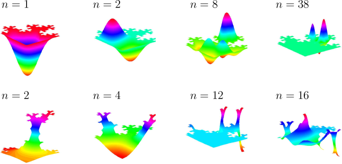
Fig. 13: Several Dirichlet (top) and Neumann (bottom) eigenfunctions for the third domain on Fig. 12 ($g=2$). The $38$th Dirichlet and the $12$th Neumann eigenfunctions are localized in a small subdomain (located in the upper right corner on Fig. 12), while the first/second Dirichlet and the $4$th Neumann eigenfunctions are almost zero on this subdomain. Finally, the $8$th Dirichlet and the second Neumann eigenfunctions are examples of eigenfunctions extended over the whole domain.

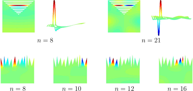
Fig. 14: Examples of localized Neumann Laplacian eigenfunctions in two domains adapted from [175]: square with many elongated holes (top) and random sawteeth (bottom). Colors represent the amplitude of eigenfunctions, from the most negative value (dark blue), through zero (green), to the largest positive value (dark red). One can notice that the eigenfunctions on the top are not negligible outside the localization region. This is yet another illustration for the conventional character of localization in bounded domains.

A number of mathematical studies were devoted to the theory of partial differential equations on fractals in general and to localization of Laplacian eigenfunctions in particular (see [280, 477] and references therein). For instance, the spectral properties of the Laplace operator on Sierpinski gasket and its extensions were thoroughly investigated [42, 43, 456, 197, 44, 46, 75]. Barlow and Kigami studied the localized eigenfunctions of the Laplacian on a more general class of self-similar sets (so-called post critically finite self-similar sets, see [281, 282] for details). They related the asymptotic behavior of the eigenvalue counting function to the existence of localized eigenfunctions and established a number of sufficient conditions for the existence of a localized eigenfunction in terms of the symmetries of a set [45].

Berry and co-workers developed a new method to approximate the Neumann spectrum of the Laplacian on a planar fractal set $\Omega$ as a renormalized limit of the Neumann spectra of the standard Laplacian on a sequence of domains that approximate $\Omega$ from the outside [66]. They applied this method to compute the Neumann-Laplacian eigenfunctions in several domains, including a sawtooth domain, Sierpinski gasket and carpet, as well as nonsymmetric and random carpets and the octagasket. In particular, they gave a numerical evidence for the localized eigenfunctions for a sawtooth domain, in agreement with the earlier work by Félix et al. [175].

Heilman and Strichartz reported several numerical examples of localized Neumann-Laplacian eigenfunctions in two domains [233], one of them is illustrated on Fig. 15a. Each of these domains consists of two subdomains with a narrow but not too narrow connection. This is a kind of dumbbell shape with a connector of zero length. Heilman and Strichartz argued that one subdomain must possess an axis of symmetry for getting localized eigenfunctions. Since an anti-symmetric eigenfunction vanishes on the axis of symmetry, it is necessarily small near the bottle-neck that somehow “prevents” its extension to the other domain. Although the argument is plausible, we have to stress that such a symmetry is neither sufficient, nor necessary for localization. It is obviously not sufficient because even for symmetric domain, there exist plenty of extended eigenfunctions (including the trivial example of the ground eigenmode which is a constant over the whole domain). In order to illustrate that the reflection symmetry is not necessary, we plot on Fig. 15b,c examples of localized eigenfunctions for modified domains for which the symmetry is broken. Although rendering the upper domain less and less symmetric gradually reduces or even fully destroys localization (Fig. 15d), its “mechanism” remains poorly understood. We also note that methods of Sec. 7.4 are not applicable in this case because of Neumann boundary condition.

Lapidus and Pang studied the boundary behavior of the Dirichlet Laplacian eigenfunctions and their gradients on a class of planar domains with fractal boundary, including the triangular and square von Koch snowflakes and their polygonal approximations [305]. A numerical evidence for the boundary behavior of eigenfunctions was reported in [307], with numerous pictures of eigenfunctions. Later, Daubert and Lapidus considered more specifically the localization character of eigenfunctions in von Koch domains [145]. In particular, different “measures” of localization were discussed.

Note also that Filoche and Mayboroda studied the problem of localization for bi-Laplacian in rigid thin plates and discovered that clamping just one point inside such a plate not only perturbs its spectral properties, but essentially divides the plate into two independently vibrating regions [185].

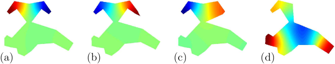
Fig. 15: Neumann-Laplace eigenfunction $u_{4}$ in the original “cow” domain from [233] (a) and in three modified domains (b,c,d), in which the reflection symmetry of the upper subdomain is broken. The fourth eigenfunction is localized for the first three domains (a,b,c), while the last domain with the strongest modification shows no localization (d). Colors represent the amplitude of an eigenfunction, from the most negative value (dark blue), through zero (green), to the largest positive value (dark red).

7.7 High-frequency localization

A hundred years ago, Lord Rayleigh documented an interesting acoustical phenomenon in the whispering gallery under the dome of Saint Paul’s Cathedral in London [419] (see also [415, 416]). A whisper of one person propagated along the curved wall to another person stood near the wall. Keller and Rubinow discussed the related “whispering gallery modes” and also “bouncing ball modes”, and showed that these modes exist for a two-dimensional domain with arbitrary smooth convex curve as its boundary [277]. A semiclassical approximation of Laplacian eigenfunctions in convex domains was developed by Lazutkin [33, 311, 312, 313, 314] (see also [13, 467, 413, 414]). Chen and co-workers analyzed Mathieu and modified Mathieu functions and reported another type of localization named “focusing modes” [126]. All these eigenmodes become more and more localized in a small subdomain when the associated eigenvalue increases. This so-called high-frequency or high-energy limit was intensively studied for various domains, named as quantum billiards [222, 235, 474, 254, 447]. In quantum mechanics, this limit is known as semi-classical approximation [61]. In optics, it corresponds to ray approximation of wave propagation, from which the properties of an optical, acoustical or quantum system can often be reduced to the study of rays in classical billiards. Jakobson et al. gave an overview of many results on geometric properties of the Laplacian eigenfunctions on Riemannian manifolds, with a special emphasis on high-frequency limit (weak star limits, the rate of growth of $L_{p}$ norms, relationships between positive and negative parts of eigenfunctions, etc.) [254] (see also [486, 4]). Bearing in mind this comprehensive review, we start by illustrating the high-frequency localization and the related problems in simple domains such as disk, ellipse and rectangle for which explicit estimates are available. After that, some results for quantum billiards are summarized.

7.7.1 Whispering gallery and focusing modes

The disk is the simplest shape for illustrating the whispering gallery and focusing modes. The explicit form (21) of eigenfunctions allows one to get accurate estimates and bounds, as shown below. When the index $k$ is fixed and $n$ increases, the Bessel functions $J_{n}(\alpha_{nk}r/R)$ become strongly attenuated near the origin (as $J_{n}(z)\sim(z/2)^{n}/n!$ at small $z$) and essentially localized near the boundary, yielding whispering gallery modes. In turn, when $n$ is fixed and $k$ increases, the Bessel functions rapidly oscillate, the amplitude of oscillations decreasing towards the boundary. In that case, the eigenfunctions are mainly localized at the origin, yielding focusing modes.

These qualitative arguments were rigorously formulated in [370]. For each eigenfunction $u_{nk}$ on the unit disk $\Omega$, one introduces the subdomain $\Omega_{nk}=\{x\in{\mathbb{R}}^{2}~{}:~{}|x|<d_{n}/\alpha_{nk}\}\subset\Omega$, where $d_{n}=n-n^{2/3}$, and $\alpha_{nk}$ are, depending on boundary conditions, the positive zeros of either $J_{n}(z)$ (Dirichlet), or $J^{\prime}_{n}(z)$ (Neumann) or $J^{\prime}_{n}(z)+hJ_{n}(z)$ for some $h>0$ (Robin), with $n=0,1,2,...$ denoting the order of Bessel function $J_{n}(z)$ and $k=1,2,3,...$ counting zeros. Then for any $p\geq 1$ (including $p=\infty$), there exists a universal constant $c_{p}>0$ such that for any $k=1,2,3,...$ and any large enough $n$, the Laplacian eigenfunction $u_{nk}$ for Dirichlet, Neumann or Robin boundary condition satisfies

$$\frac{\|u_{nk}\|_{L_{p}(\Omega_{nk})}}{\|u_{nk}\|_{L_{p}(\Omega)}}<c_{p}n^{\frac{1}{3}+\frac{2}{3p}}\exp(-n^{1/3}\ln(2)/3).$$ (98)

The definition of $\Omega_{nk}$ and the above estimate imply

$$\lim\limits_{n\to\infty}\frac{\|u_{nk}\|_{L_{p}(\Omega_{nk})}}{\|u_{nk}\|_{L_{p}(\Omega)}}=0,\hskip 28.45274pt\lim\limits_{n\to\infty}{\frac{\mu_{2}(\Omega_{nk})}{\mu_{2}(\Omega)}}=1.$$ (99)

This theorem shows the existence of infinitely many Laplacian eigenmodes which are $L_{p}$-localized in a thin layer near the boundary $\partial\Omega$. In fact, for any prescribed thresholds for both ratios in (88), there exists $n_{0}$ such that for all $n>n_{0}$, the eigenfunctions $u_{nk}$ are $L_{p}$-localized. These eigenfunctions are called “whispering gallery eigenmodes” and illustrated on Fig. 16.

We outline a peculiar relation between high-frequency and low-frequency localization. The explicit form (21) of Dirichlet Laplacian eigenfunctions $u_{nk}$ leads to their simple nodal structure which is formed by $2n$ radial nodal lines and $k-1$ circular nodal lines. The radial nodal lines split the disk into $2n$ circular sectors with Dirichlet boundary conditions. As a consequence, whispering gallery eigenmodes in the disk and the underlying exponential estimate (98) turn out to be related to the exponential decay of eigenfunctions in domains with branches (Sec. 7.4), as illustrated on Fig. 8 for elongated triangles.

A simple consequence of the above theorem is that for any $p\geq 1$ and any open subset $V$ compactly included in the unit disk $\Omega$ (i.e., $\bar{V}\cap\partial\Omega=\emptyset$), one has

$$\lim\limits_{n\to\infty}\frac{\|u_{nk}\|_{L_{p}(V)}}{\|u_{nk}\|_{L_{p}(\Omega)}}=0,$$ (100)

and

$$C_{p}(V)\equiv\inf\limits_{nk}\left\{\frac{\|u_{nk}\|_{L_{p}(V)}}{\|u_{nk}\|_{L_{p}(\Omega)}}\right\}=0.$$ (101)

Qualitatively, for any subset $V$, there exists a sequence of eigenfunctions that progressively “escape” $V$.

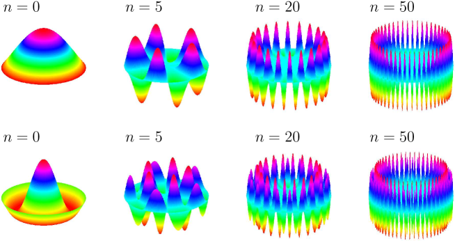
Fig. 16: Formation of whispering gallery modes for the unit disk with Dirichlet boundary condition: for a fixed $k$ ($k=1$ for top figures and $k=2$ for bottom figures), an increase of the index $n$ leads to stronger localization of eigenfunctions near the boundary.

The localization of focusing modes at the origin is revealed in the limit $k\to\infty$. For each $R\in(0,1)$, one defines an annulus $\Omega_{R}=\{x\in{\mathbb{R}}^{2}~{}:~{}R<|x|<1\}\subset\Omega$ of the unit disk $\Omega$. Then, for any $n=0,1,2,...$, the Laplacian eigenfunction $u_{nk}$ with Dirichlet, Neumann or Robin boundary condition satisfies

$$\lim\limits_{k\to\infty}\frac{\|u_{nk}\|_{L_{p}(\Omega_{R})}}{\|u_{nk}\|_{L_{p}(\Omega)}}=\begin{cases}(1-R^{2-p/2})^{1/p}\quad(1\leq p<4),\cr\hskip 28.45274pt0\hskip 62.59605pt(p>4).\end{cases}$$ (102)

When the index $k$ increases (with fixed $n$), the eigenfunctions $u_{nk}$ become more and more $L_{p}$-localized near the origin when $p>4$ [370]. These eigenfunctions are called “focusing eigenmodes” and illustrated on Fig. 17. The theorem shows that the definition of localization is sensitive to the norm: the above focusing modes are $L_{p}$-localized for $p>4$, but they are not $L_{p}$-localized for $p<4$. Similar results for whispering gallery and focusing modes hold for a ball in three dimensions [370].

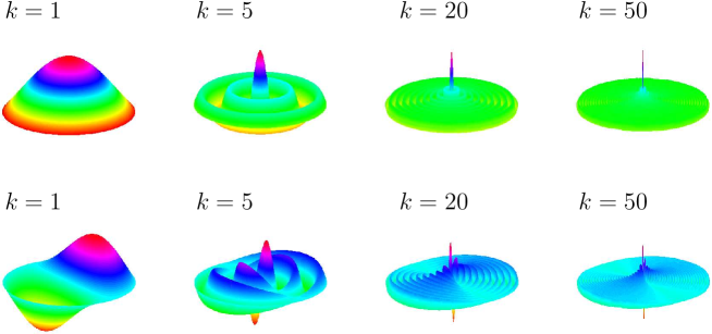
Fig. 17: Formation of focusing modes for the unit disk with Dirichlet boundary condition: for a fixed $n$ ($n=0$ for top figures and $n=1$ for bottom figures), an increase of the index $k$ leads to stronger localization of eigenfunctions at the origin.

7.7.2 Bouncing ball modes

Filled ellipses and elliptical annuli are simple domains for illustrating bouncing ball modes. For fixed foci (i.e., a given parameter $a$ in the elliptic coordinates in Eq. (27)), these domains are characterized by two radii, $R_{0}$ ($R_{0}=0$ for filled ellipses) and $R$, as $\Omega=\{(r,\theta)~{}:~{}R_{0}<r<R,~{}0\leq\theta<2\pi\}$, while the eigenfunctions $u_{nkl}$ were defined in Sec. 3.4. For each $\alpha\in\left(0,\frac{\pi}{2}\right)$, we consider an elliptical sector $\Omega_{\alpha}$ inside an elliptical domain $\Omega$ (Fig. 2)

$$\Omega_{\alpha}=\left\{(r,\theta)~{}:~{}R_{0}<r<R,~{}\theta\in(\alpha,\pi-\alpha)\cup(\pi+\alpha,2\pi-\alpha)\right\}.$$

For any $p\geq 1$, there exists $\Lambda_{\alpha,n}>0$ such that for any eigenvalue $\lambda_{nkl}>\Lambda_{\alpha,n}$, the corresponding eigenfunction $u_{nkl}$ satisfies [370] (see also [68])

$$\frac{\left\|u_{nkl}\right\|_{L_{p}(\Omega\setminus\Omega_{\alpha})}}{\left\|u_{nkl}\right\|_{L_{p}(\Omega)}}<D_{n}\left(\frac{16\alpha}{\pi-\alpha/2}\right)^{1/p}\exp\left(-a\sqrt{\lambda_{nkl}}\left[\sin\left(\frac{\pi}{4}+\frac{\alpha}{2}\right)-\sin\alpha\right]\right),$$ (103)

where

$$D_{n}=3\sqrt{\frac{1+\sin\left({\frac{3\pi}{8}+\frac{\alpha}{4}}\right)}{\bigl{[}\tan\left({\frac{\pi}{16}-\frac{\alpha}{8}}\right)\bigr{]}^{n}}}.$$

Given that $\lambda_{nkl}\to\infty$ as $k$ increases (for any fixed $n$ and $l$), while the area of $\Omega_{\alpha}$ can be made arbitrarily small by sending $\alpha\to\pi/2$, the estimate implies that there are infinitely many eigenfunctions $u_{nkl}$ which are $L_{p}$-localized in the elliptical sector $\Omega_{\alpha}$:

$$\lim\limits_{k\to\infty}\frac{\|u_{nkl}\|_{L_{p}(\Omega\setminus\Omega_{\alpha})}}{\|u_{nkl}\|_{L_{p}(\Omega)}}=0.$$ (104)

These eigenfunctions, which are localized near the minor axis, are called “bouncing ball modes” and illustrated on Fig. 18. The above estimate allows us to illustrate bouncing ball modes which are known to emerge for any convex planar domain with smooth boundary [277, 126]. At the same time, the estimate is as well applicable to elliptical annuli, providing thus an example of bouncing ball modes for non-convex domains.

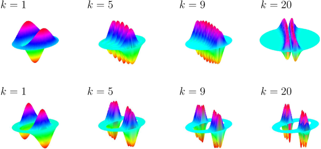
Fig. 18: Formation of bouncing ball modes $u_{nkl}$ in a filled ellipse of radius $R=1$ (top) and an elliptical annulus of radii $R_{0}=0.5$ and $R=1$ (bottom), with the focal distance $a=1$, and Dirichlet boundary condition. For fixed $n=1$ and $l=1$, an increase of the index $k$ leads to stronger localization of the eigenfunction near the vertical semi-axis (from [370]).

7.7.3 Domains without localization

The analysis of geometrical properties of eigenfunctions in rectangle-like domains $\Omega=(0,\ell_{1})\times...\times(0,\ell_{d})\subset{\mathbb{R}}^{d}$ (with sizes $\ell_{1}>0$, …, $\ell_{d}>0$) may seem to be the simplest case because the eigenfunctions are expressed through sines (Dirichlet) and cosines (Neumann), as discussed in Sec. 3.1. The situation is indeed elementary when all eigenvalues are simple, i.e., $(\ell_{i}/\ell_{j})^{2}$ are not rational numbers for all $i\neq j$. For any $p\geq 1$ and any open subset $V\subset\Omega$, one can prove that [370]

$$C_{p}(V)\equiv\inf\limits_{n_{1},...,n_{d}}\left\{\frac{\|u_{n_{1},...,n_{d}}\|_{L_{p}(V)}}{\|u_{n_{1},...,n_{d}}\|_{L_{p}(\Omega)}}\right\}>0.$$ (105)

This property is in sharp contrast to Eq. (101) for eigenfunctions in the unit disk (or ball). The fact that $C_{p}(V)>0$ for any open subset $V$ means that there is no eigenfunction that could fully “avoid” any location inside the domain, i.e., there is no $L_{p}$-localized eigenfunction. Since the set of rational numbers has zero Lebesgue measure, there is no $L_{p}$-localized eigenfunctions in almost any randomly chosen rectangle-like domain.

When at least one ratio $(\ell_{i}/\ell_{j})^{2}$ is rational, certain eigenvalues are degenerate, and the associated eigenfunctions are linear combinations of products of sines or cosines (see Sec. 3.1). Although the computation is still elementary for each eigenfunction, it is unknown whether the infimum $C_{p}(V)$ from Eq. (105) is strictly positive or not, for arbitrary rectangle-like domain $\Omega$ and any open subset $V$. For instance, the most general known result for a rectangle $\Omega=(0,\ell_{1})\times(0,\ell_{2})$ states that $C_{2}(V)>0$ for any $V\subset\Omega$ of the form $V=(0,\ell_{1})\times\omega$, where $\omega$ is any open subset of $(0,\ell_{2})$ [110] (see also [335]). Even for the unit square, the statement $C_{p}(V)>0$ for any open subset $V$ appears as an open problem. More generally, one may wonder whether $C_{p}(V)$ is strictly positive or not for any open subset $V$ in polygonal (convex) domains.

7.7.4 Quantum billiards

The above examples of whispering gallery or bouncing ball modes illustrate that certain high-frequency eigenfunctions tend to be localized in specific regions of circular and elliptical domains. But what is the structure of a high-frequency eigenfunction in a general domain? What are these specific regions on which a sequence of eigenfunctions may be localized, and whether do localized eigenfunctions exist for a given domain? Answers to these and other related questions can be found by relating the high-frequency behavior of a quantum system (in our case, the structure of Laplacian eigenfunctions) to the classical dynamics in a billiard of the same shape [12, 327, 221, 129, 271]. This relation is also known as a semi-classical approximation in quantum mechanics and a ray approximation of wave propagation in optics, while the correspondence between classical and quantum systems can be shown by the WKB method, Eikonal equation or Feynman path integrals [361, 179, 180]. For instance, the dynamics of a particle in a classical billiard is translated into quantum mechanism through the stationary Schrödinger equation $Hu_{n}(x)=E_{n}u_{n}(x)$ with Dirichlet boundary condition, where the free Hamiltonian is $H=p^{2}/(2m)=-\hbar^{2}\Delta/(2m)$, and the energy $E_{n}$ is related to the corresponding Laplacian eigenvalue $\lambda_{n}=2mE_{n}/\hbar^{2}$. Since $|u_{n}(x)|^{2}$ is the probability density for finding a quantum particle at $x$, this density should resemble some classical trajectory of that particle in the (high-frequency) semi-classical limit ($\hbar\to 0$ or $m\to\infty$). In particular, some orbits of a particle moving in a classical billiard may appear as “scars” in the spatial structure of eigenfunctions in the related quantum billiard [234, 222, 164, 65, 31, 473, 446, 267, 235, 269, 474, 223, 254, 447]. This effect is illustrated on Fig. 19 by Liu and co-workers who investigated the localization of Dirichlet Laplacian eigenfunctions on classical periodic orbits in a spiral-shaped billiard [330] (see also [317]).

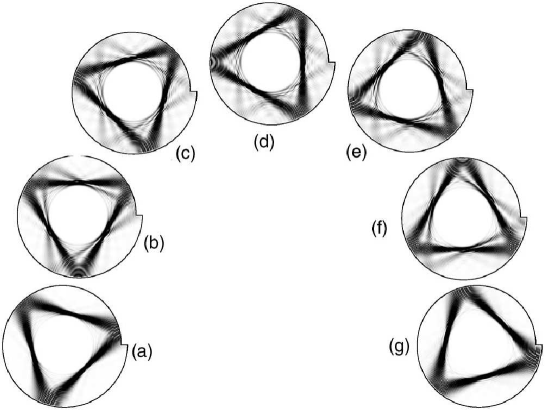
Fig. 19: Several eigenstates with localization on periodic orbits for the spiral-shaped billiard with $\epsilon=0.1$, from [330] (Reprinted Fig. 6 with permission from Liu et al., Physical Reviews E, 74, 046214, (2006). Copyright (2006) by the American Physical Society).

Fig. 20: Examples of chaotic billiards: (a) Bunimovich stadium (union of a square and two half-disks) [98, 99, 234, 483, 484, 131, 69], (b) Sinai’s billiard [463, 464], (c) mushroom billiard [100, 48], and (d) hyperbolic billiard [2]. Many other examples are given in [99].

In the classical dynamics, one may distinguish the domains with regular, integrable and chaotic dynamics. In particular, for a bounded domain $\Omega$ with an ergodic billiard flow [462], Shnirelman’s theorem (also known as quantum ergodicity theorem [136, 508, 509]) states that among the set of $L_{2}$-normalized Dirichlet (or Neumann) Laplacian eigenfunctions, there is a sequence $u_{j_{k}}$ of density $1$ (i.e., $\lim\limits_{k\to\infty}{j_{k}/k}=1$), such that for any open subset $V\subset\Omega$, one has [459]

$$\lim\limits_{k\rightarrow\infty}\int\limits_{V}|u_{j_{k}}(x)|^{2}dx=\frac{\mu_{d}(V)}{\mu_{d}(\Omega)}.$$ (106)

(this version of the theorem was formulated in [110]). Marklof and Rudnick extended this theorem to rational polygons (i.e., simple plane polygons whose interior is connected and simply connected and all the vertex angles are rational multiplies of $\pi$) [335]. Loosely speaking, $\{u_{j_{k}}\}$ is a sequence of non-localized eigenfunctions which become more and more uniformly distributed over the domain (see [254, 110, 201] for further discussion and references). At the same time, this theorem does not prevent the existence of localized eigenfunctions. How large the excluded subsequence of (localized) eigenfunctions may be? In the special case of arithmetic hyperbolic manifolds, Rudnick and Sarnak proved that there is no such excluded subsequence [432]. This statement is known as the quantum unique ergodicity (QUE). The validity of this statement for other dynamical systems (in particular, ergodic billiards) remains under investigation [159, 47, 230]. The related notion of weak quantum ergodicity was discussed by Kaplan and Heller [268]. A classification of eigenstates to regular and irregular ones was thoroughly discussed (see [409, 495] and references therein).

There were numerous studies of Laplacian eigenfunctions in chaotic domains such as, e.g., Bunimovich stadium [98, 99, 234, 375, 483, 484, 131, 69], Sinai’s billiard [463, 464], mushroom billiard [100, 48] or hyperbolic billiard [2], illustrated on Fig. 20. The literature on quantum billiards is vast, and we only mention selected works on the spatial structure of high-frequency eigenfunctions. McDonald and Kaufman studied the Bunimovich stadium billiard and reported a random structure of nodal lines of eigenfunctions and Wigner-type distribution for eigenvalue spacings [348, 349]. Bohigas and co-workers analyzed eigenvalue spacings for the Sinai’s billiard and also obtained the Wigner-type distribution [81]. It means that eigenvalue spacings for these chaotic billiards obey the same distribution as that for random matrices from the Gaussian Orthogonal Ensemble. This is in a sharp contrast to regular billiards for which eigenvalue spacings generally follow a Poisson distribution. The problem of circular-sector and related billiards was studied (e.g., see [324]).

Polygon billiards have attracted a lot of attention, especially the class of rational polygons for which all the vertex angles are rational multiples of $\pi$ [427, 325, 326]. As the dynamics in rational polygons is neither integrable nor ergodic (except several classical integrable cases such as rectangles, equilateral triangle, right triangles with an acute vertex angle $\pi/3$ or $\pi/4$), they are often called pseudo-integrable systems. Bellomo and Uzer studied scarring states in a pseudo-integrable triangular billiard and detected scars in regions which contain no periodic orbits [57]. Amar et al. gave a complete characterization of the polygons for which a Dirichlet eigenfunction can be found in terms of a finite superposition of plane waves [7, 8] (see also [310] for experimental study). Biswas and Jain investigated in detail the $\pi/3$-rhombus billiard which presents an example of the simplest pseudo-integrable system [72]. Hassell et al. proved for an arbitrary polygonal billiard that eigenfunction mass cannot concentrate away from the vertices [229] (see also [336]). The level spacing properties of rational and irrational polygons were studied numerically by Shimizu and Shudo [457]. They also analyzed the structure of the related eigenfunctions [458].

Bäcker and co-workers analyzed the number of bouncing ball modes in a class of two-dimensional quantized billiards with two parallel walls [35]. Bunimovich introduced a family of simple billiards (called “mushrooms”) that demonstrate a continuous transition from a completely chaotic system (stadium) to a completely integrable one (circle) [100]. Barnett and Betcke reported the first large-scale statistical study of very high-frequency eigenfunctions in these billiards [48]. Using nonstandard numerical techniques [47], Barnett also studied the rate of equidistribution for a uniformly hyperbolic, Sinai-type, planar Euclidean billiard with Dirichlet boundary condition, as illustrated on Fig. 21. This study brought a strong numerical evidence for the QUE in this system. The spatial structure of high-frequency eigenfunctions shown on Fig. 21 looks somewhat random. This observation goes back to Berry who conjectured that high-frequency eigenfunctions in domains with ergodic flow should look locally like a random superposition of plane waves with a fixed wavenumber [62]. This analogy is illustrated on Fig. 22 by Barnett [47]. O’Connor and co-workers analyzed the random pattern of ridges in a random superposition of plane waves [374].

Pseudo-integrable barrier billiards were intensively studied in a series of theoretical, numerical and experimental works by Bogomolny et al. [79, 80]. They reported on the emergence of scarring eigenstates which are related with families of classical periodic orbits that do not disappear at large quantum numbers in contrast to the case of chaotic systems. These so-called superscars were observed experimentally in a flat microwave billiard with a barrier inside [80]. Wiersig performed an extensive numerical study of nearest-neighbor spacing distributions, next-to-nearest spacing distributions, number variances, spectral form factors, and the level dynamics [503]. Dietz and co-workers analyzed the number of nodal domains in a barrier billiard [156].

Tomsovic and Heller verified a remarkable accuracy of the semi-classical approximation that relates the classical and quantum billiards [483, 484]. In some cases, eigenfunctions can therefore be constructed by purely semiclassical calculations. Li et al. studied the spatial distribution of eigenstates of a rippled billiard with sinusoidal walls [322]. For this type of ripple billiards, a Hamiltonian matrix can be found exactly in terms of elementary functions that greatly improves computation efficiency. They found both localized and extended eigenfunctions, as well as peculiar hexagon and circle-like pattern formations. Frahm and Shepelyansky considered almost circular billiards with a rough boundary which was realized as a random curve with some finite correlation length. On a first glance it may seem that such a rough boundary in a circular billiard would destroy the conservation of angular momentum and lead to ergodic eigenstates and the level statistics predicted by random matrix theory. They showed, however, that there is a region of roughness in which the classical dynamics is chaotic but the eigenstates are localized [190]. Bogomolny et al. presented the exact computation of the nearest-neighbor spacing distribution for a rectangular billiard with a pointlike scatterer inside [78].

Prosen computed numerically very high-lying energy spectra for a generic chaotic 3D quantum billiard (a smooth deformation of a unit sphere) and analyzed Weyl’s asymptotic formula and the nearest neighbor level spacing distribution. He found significant deviations from the Gaussian Orthogonal Ensemble statistics that were explained in terms of localization of eigenfunctions onto lower dimensional classically invariant manifolds [410]. He also found that the majority of eigenstates were more or less uniformly extended over the entire energy surface, except for a fraction of strongly localized scarred eigenstates [411]. An extensive study of 3D Sinai’s billiard was reported by Primack and Smilansky [408]. Deviations from a semi-classical description were discussed by Tanner [481]. Casati and co-workers investigated how the interplay between quantum localization and the rich structure of the classical phase space influences the quantum dynamics, with applications to hydrogen atoms under microwave fields [119, 120, 121, 122] (see also references therein).

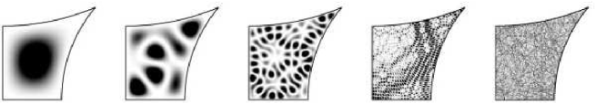
Fig. 21: Illustration of spatial distribution of the Dirichlet Laplacian eigenfunction $|u_{m}|^{2}$ (shown as density plots: larger values are darker) with $m=1,10,100,1000$ and $m\approx 50000$ [47] (by A. Barnett, with permission).

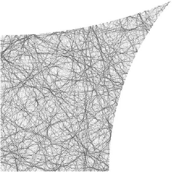
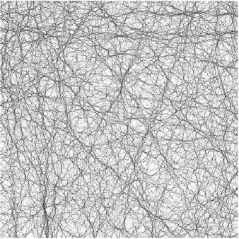
Fig. 22: (Left) Density plot of a Dirichlet-Laplacian eigenfunction $|u_{m}|^{2}$ for $m\approx 50000$ with the eigenvalue $\lambda_{m}\approx 10^{6}$. There are about 225 wavelengths across the diagonal; (Right) Density plot of one sample from the ensemble of random plane waves with the same wavenumber and mean intensity, shown in a square region of space (with no boundary conditions) [47] (by A. Barnett, with permission).

A large number of physical experiments were performed with classical and quantum billiards. For instance, Gräf and co-workers measured more than thousand first eigenmodes in a quasi two-dimensional superconducting microwave stadium billiard with chaotic dynamics [210]. Sridhar and co-workers performed a series of experiments in microwave cavities in the shape of Sinai’s billiard [469, 470]. In particular, they observed bouncing ball modes and modes with quasi-rectangular or quasi-circular symmetry which are associated with nonisolated periodic orbits (which avoid the central disk). Some scarring eigenstates, which are associated with isolated periodic orbits (which hit the central disk, see Fig. 20b), were also observed. Kudrolli et al. investigated the signatures of classical chaos and the role of periodic orbits in the eigenvalue spectra of two-dimensional billiards through experiments in microwave cavities [297, 298]. The eigenvalue spectra were analyzed by using the nearest neighbor spacing distribution for short-range correlations and the spectral rigidity for longer-range correlations. The density correlation function was used for studying the spatial structure of eigenstates. The role of disorder was also investigated. Chinnery and Humphrey visualized experimentally acoustic resonances within a stadium-shaped cavity [131]. Bittner et al. performed double-slit experiments with regular and chaotic microwave billiards [73]. Chaotic resonators were also employed for getting specific properties of lasers (e.g., high-power directional emission or “Fresnel filtering”) [205, 425].

8 Other points and concluding remarks

This review was focused on the geometrical properties of Laplacian eigenfunctions in Euclidean domains. We started from the basic properties of the Laplace operator and explicit representations of its eigenfunctions in simple domains. After that, the properties of eigenvalues and their relation to the shape of a domain were briefly summarized, including Weyl’s asymptotic behavior, isoperimetric inequalities, and Kac’s inverse spectral problem. The structure of nodal domains and various estimates for the norms of eigenfunctions were then presented. The main Section 7 was devoted to the spatial structure of eigenfunctions, with a special emphasis on their localization in small subsets of a domain. One of the major difficulties in the study of localization is that localization is a property of an individual eigenfunction. For the same domain, two consecutive eigenfunctions with very close eigenvalues may have drastically different geometrical structures (e.g., one is localized and the other is extended). One needs therefore fine analytical tools which would differently operate with localized and non-localized eigenfunctions. In the review, we distinguished two types of localization, for low-frequency and high-frequency eigenfunctions.

In the former case, an eigenfunction remains localized in a subset because of a geometric constraint that prohibits its extension to other parts of the domain. A standard example is a dumbbell (two domains connected by a narrow channel), for which an eigenfunction may be localized in one domain if its typical wavelength is larger than the width of the channel (meaning that an eigenfunction cannot “squeeze” through the channel). Such kind of “expulsion” from a channel is quite generic, as the analysis is applicable to domains with branches of variable cross-sectional profiles. It is important to note that a geometric constraint does not need to be strong (e.g., two domains may be separated by a cloud of point-like obstacles of zero measure). Another example is an elongated triangle, in which there is no “obstacles” at all. Low-frequency localization was found numerically in many irregularly-shaped domains, for both Dirichlet and Neumann boundary conditions. From a practical point of view, the low-frequency localization may find various applications, e.g., it is important for the theory of quantum, optical and acoustical waveguides and microelectronic devices, as well as for analysis and engineering of highly reflecting or absorbing materials (noise protective barriers, anti-radar coatings, etc).

The high-frequency localization manifests in quantum billiards when a sequence of eigenfunctions tends to concentrate onto some orbits of the associated classical billiard. In this regime, the asymptotic properties of eigenvalues and eigenfunctions are strongly related to the underlying classical dynamics (e.g., regular, integrable or chaotic). For instance, the ergodic character of the classical system is reflected in the spatial structure of eigenfunctions. Working on simple domains, we illustrated several kinds of localized eigenfunctions which emerge for a large class of domains. We also provided examples of rectangular domains without localization. Although a number of rigorous and numerical results were obtained (e.g., quantum ergodicity theorem for ergodic billiards), many questions about the spatial structure of high-frequency eigenfunctions remain open, even for very simple domains (e.g., a square).

Although the review counts more than five hundred citations, it is far from being complete. As already mentioned, we focused on the Laplace operator in bounded Euclidean domains and mostly omitted technical details, in order to keep the review at a level accessible to scientists from various fields. Many other issues had to be omitted:

(i) Many important results for Laplacians on Riemannian manifolds or weighted graphs could not be included. In addition, we did not discuss the spectral properties of domains with “holes” [439, 381, 340, 341, 497, 188, 382, 448, 287, 130, 302], as well as their consequences for diffusion in domains with static traps [211, 275, 276, 485, 369]. The behavior of the eigenvalues and eigenfunctions under deformations of a domain was partly considered in Sec. 6.1 and Sec. 7.5, while many significant results were not included (see [423, 270, 461, 91, 279] and references therein).

(ii) There are important developments of numerical techniques for computing the Laplacian eigenbasis. In fact, standard finite difference or finite element methods rely on a regular or adapted discretization of a domain that reduces the continuous eigenvalue problem to a finite set of linear equations [134, 435, 299, 141, 242, 193, 218]. Since finding the eigenbasis of the resulting matrix is still an expensive computational task, various hints and tricks are often implemented. For instance, for planar polygonal domains, one can exploit the behavior of eigenfunctions at corners through radial basis functions in polar coordinates and the integration of related Fourier-Bessel functions on subdomains [153, 162, 398]. Another “trick” is conformal mapping of planar polygonal domains onto the unit disk, for which the modified eigenvalue problem can be efficiently solved [37, 38]. Yet another approach, known as the method of particular solutions was suggested by Fox and co-workers [189] and later progressively improved [34, 67, 49]. The main idea is to consider various solutions of the eigenvalue equation for a given value of $\lambda$ and to vary $\lambda$ until a linear combination of such solutions would satisfy the boundary condition at a number of sample points along the boundary. One can also mention a stochastic method by Lejay and Maire for computing the principal eigenvalue [318]. The eigenvalue problem can also be reformulated in terms of boundary integral equations that reduces the dimensionality and allows for rapid computation of eigenvalues [332]. Kaufman and co-workers proposed a simple expansion method in which wave functions inside a two-dimensional quantum billiard are expressed in terms of an expansion of a complete set of orthonormal functions defined in a surrounding rectangle for which Dirichlet boundary conditions apply, while approximating the billiard boundary by a potential energy step of a sufficiently large size [273]. Vergini and Saraceno proposed a scaling method for computing high-frequency eigenmodes [496]. This method was later improved by Barnett and Hassell [50] (this reference is also a good review of numerical methods for high-frequency Dirichlet Laplacian eigenvalues).

(iii) We did not discuss various applications of Laplacian eigenfunctions which nowadays range from pure and applied mathematics to physics, chemistry, biology and computer sciences. One can mention manifold parameterizations by Laplacian eigenfunctions and heat kernels [265], the use of Laplacian spectra as a diagnostic tool for network structure and dynamics [350], efficient image recognition and analysis [424, 436, 437, 426], shape optimization and spectral partition problems [397, 468, 6, 94, 113, 114, 494], computation and analysis of diffusion-weighted NMR signals [213, 214, 215], localization in heterogeneous materials (e.g., photonic crystals) and the related optimization problem [262, 263, 181, 182, 183, 184, 285, 286, 296, 158, 438, 294], etc.

References

- [1] M. Abramowitz and I. A. Stegun, Handbook of Mathematical Functions, Dover Publisher, New York, 1965.
- [2] O. Agam and S. Fishman, Semiclassical criterion for scars of wavefunctions in chaotic systems, Phys. Rev. Lett. 73 (1994), pp. 806-809.
- [3] S. Agmon, Lectures on Exponential Decay of Solution of Second-Order Elliptic Equation, Princeton University Press, 1982.
- [4] J. H. Albert, Generic properties of eigenfunctions of elliptic partial differential operators, Trans. Amer. Math. Soc. 238 (1978), pp. 341-354.
- [5] G. Alessandrini, Nodal lines of eigenfunctions of the fixed membrane problem in general convex domains, Comment. Math. Helv. 69 (1994), pp. 142-154.
- [6] G. Allaire, Shape Optimization by the Homogenization Method, Applied Mathematical Sciences 146, Springer-Verlag, New York, 2002.
- [7] V. Amar, M. Pauri, and A. Scotti, Schrödinger equation for convex plane polygons: A tiling method for the derivation of eigenvalues and eigenfunctions, J. Math. Phys. 32 (1991), pp. 2442-2449.
- [8] V. Amar, M. Pauri, and A. Scotti, Schrödinger equation for convex plane polygons. II. A no-go theorem for plane waves representation of solutions, J. Math. Phys. 34 (1993), pp. 3343.
- [9] P. W. Anderson, Absence of Diffusion in Certain Random Lattices, Phys. Rev. 109 (1958), pp. 1492-1505.
- [10] B. Andrews and J. Clutterbuck, Proof of the fundamental gap conjecture, J. Am. Math. Soc. 24 (2011), pp. 899-916.
- [11] W. Arendt, R. Nittka, W. Peter and F. Steiner, Weyl’s Law: Spectral Properties of the Laplacian in Mathematics and Physics, in “Mathematical Analysis of Evolution, Information, and Complexity”, Eds. by W. Arendt and W. P. Schleich, Wiley-VCH Verlag, 2009.
- [12] V. I. Arnold, Mathematical Methods of Classical Mechanics, New York, 1978.
- [13] V. I. Arnold, Modes and quasimodes, Funct. Anal. Appl. 6 (1972), pp. 94-101.
- [14] J. M. Arrieta, Rates of eigenvalues on a dumbbell domain, simple eigenvalue case Trans. Am. Math. Soc. 347 (1995), pp. 3503-3531.
- [15] J. M. Arrieta, Neumann eigenvalue problems on exterior perturbations of the domain, J. Diff. Eq. 118 (1995), pp. 54-103.
- [16] J. M. Arrieta, A. N. Carvalho, and G. Lozada-Cruz, Dynamics in dumbbell domains I. Continuity of the set of equilibria, J. Diff. Eq. 231 (2006), pp. 551-597.
- [17] J. M. Arrieta, A. N. Carvalho, and G. Lozada-Cruz, Dynamics in dumbbell domains II. The limiting problem, J. Diff. Eq. 247 (2009), pp. 174-202.
- [18] J. M. Arrieta, A. N. Carvalho, and G. Lozada-Cruz, Dynamics in dumbbell domains III. Continuity of attractors, J. Diff. Eq. 247 (2009), pp. 225-259.
- [19] J. M. Arrieta and D. Krejčiřík, Geometric versus spectral convergence for the Neumann Laplacian under exterior perturbations of the domain, Integral methods in science and engineering. Vol. 1, 9-19, Birkhäuser Boston, MA, 2010.
- [20] Y. Asada, K. Slevin and T. Ohtsuki, Anderson Transition in Two-Dimensional Systems with Spin-Orbit Coupling, Phys. Rev. Lett. 89 (2002), 256601.
- [21] Y. Asada, K. Slevin and T. Ohtsuki, Numerical estimation of the function in two-dimensional systems with spin-orbit coupling, Phys. Rev. B 70 (2004), 035115.
- [22] M. S. Ashbaugh and P. Exner, Lower bounds to bound state energies in bent tubes, Phys. Lett. A 150 (1990), pp. 183-186.
- [23] M. S. Ashbaugh and R. D. Benguria, Proof of the Payne-Pólya-Weinberger conjecture, Bull. Amer. Math. Soc. 25 (1991), pp. 19-29.
- [24] M. S. Ashbaugh and R. D. Benguria, A sharp bound for the ratio of the first two eigenvalues of Dirichlet Laplacians and extensions, Ann. Math. 135 (1992), pp. 601-628.
- [25] M. S. Ashbaugh and R. D. Benguria, Universal Bounds for the Low Eigenvalues of Neumann Laplacians in n Dimensions, SIAM J. Math. Anal. 24 (1993), pp. 557-570.
- [26] M. S. Ashbaugh and R. D. Benguria, More bounds on eigenvalue ratios for Dirichlet Laplacians in n dimensions, SIAM J. Math. Anal. 24 (1993), pp. 1622-1651.
- [27] M. Ashbaugh, Isoperimetric and Universal Inequalities for Eigenvalues, in “Spectral Theory and Geometry, ICMS Instructional Conference, Edinburgh 1998, Eds. by E. B. Davies, Yu. Safarov, Cambridge Univ. Press, 1999, pp. 95-139 [online on ArXiv: math.SP 0008087 (2000)].
- [28] M. S. Ashbaugh, The Fundamental Gap, unpublished write-up for the AIMS meeting in May 2006, freely available online at http://www.aimath.org/WWN/loweigenvalues/gap.pdf
- [29] M. S. Ashbaugh and R. D. Benguria, Isoperimetric Inequalities for Eigenvalues of the Laplacian, Proc. Symp. Pure Math. 76 (2007), pp. 105-139.
- [30] M. S. Ashbaugh, A. Henrot and R. S. Laugesen, Rebuttal of Donnelly’s paper on the spectral gap, Math. Z. 269 (2011), pp. 5-7.
- [31] R. Aurich and F. Steiner, Exact theory for the quantum eigenstates of a strongly chaotic system, Physica D 48 (1991), pp. 445-470.
- [32] Y. Avishai, D. Bessis, B. G. Giraud, and G. Mantica, Quantum bound states in open geometries, Phys. Rev. B 44 (1991), pp. 8028-8034.
- [33] V. Babich and V. Lazutkin, Eigenfunctions concentrated near a closed geodesic, Topics in Math. Phys., vol. 2 (M. Sh. Birman, ed.), Consultants Bureau, New York 1968, pp. 9-18.
- [34] A. Bäcker, Numerical aspects of eigenvalue and eigenfunction computations for chaotic quantum systems, in The mathematical aspects of quantum maps, vol. 618 of Lecture Notes in Physics, Springer, Berlin, 2003, pp. 91-144.
- [35] A. Bäcker, R. Schubert, and P. Stifter, On the number of bouncing ball modes in billiards, J. Phys. A 30 (1997), pp. 6783-6795.
- [36] C. Bandle, Isoperimetric Inequalities and Applications, Pitman, London 1980.
- [37] L. Banjai and L. N. Trefethen, A Multipole Method for Schwarz-Christoffel Mapping of Polygons with Thousands of Sides, SIAM J. Sci. Comput. 25 (2003), pp. 1042-1065.
- [38] L. Banjai, Eigenfrequencies of fractal drums, J. Comput. Appl. Math. 198 (2007), pp. 1-18.
- [39] R. Banuelos and T. Carroll, Brownian motion and the fundamental frequency of a drum, Duke Math. J. 75 (1994), pp. 575-602.
- [40] R. Banuelos, Sharp estimates for Dirichlet eigenfunctions in simply connected domains, J. Diff. Eq. 125 (1996), pp. 282-298.
- [41] R. Banuelos and K. Burdzy, On the “hot spots” conjecture of J. Rauch, J. Funct. Anal. 164 (1999), pp. 1-33.
- [42] M. T. Barlow and E. A. Perkins, Brownian motion on the Sierpinski gasket, Probab. Theory Related Fields 79 (1988), pp. 542-624.
- [43] M. T. Barlow and R. F. Bass, The Construction of Brownian Motion on the Sierpinski Carpet, Ann. Inst. H. Poincaré Probab. Statist. 25 (1989), pp. 225-257.
- [44] M. T. Barlow, Diffusions on Fractals, In Lectures on Probability Theory and Statistics (Saint-Flour, 1995), Lecture Notes in Math. 1690, Berlin, Springer, 1998, pp. 1-121.
- [45] M. T. Barlow and J. Kigami, Localized eigenfunctions of the Laplacian on p.c.f. self-similar sets, J. London Math. Soc. 56 (1997), pp. 320-332.
- [46] M. T. Barlow and R. F. Bass, Brownian Motion and Harmonic Analysis on Sierpinski Carpets, Canad. J. Math. 51 (1999), pp. 673-744.
- [47] A. H. Barnett, Asymptotic rate of quantum ergodicity in chaotic Euclidean billiards, Comm. Pure Appl. Math. 59 (2006), pp. 1457-1488.
- [48] A. H. Barnett and T. Betcke, Quantum mushroom billiards, Chaos 17 (2007), 043125.
- [49] A. H. Barnett, Perturbative analysis of the method of particular solutions for improved inclusion of high-lying Dirichlet eigenvalues, SIAM J. Num. Anal. 47 (2009), pp. 1952-1970.
- [50] A. Barnett and A. Hassell, Fast computation of high frequency Dirichlet eigenmodes via the spectral flow of the interior Neumann-to-Dirichlet map, submitted to Comm. Pure Appl. Math. 2012 (available on Arxiv:1112.5665).
- [51] R. F. Bass, Diffusions and Elliptic Operators, Springer, New York, 1998.
- [52] R. F. Bass, Probabilistic Techniques in Analysis, Probab. Appl., Springer, New York, 1995.
- [53] R. F. Bass and K. Burdzy, On Domain Monotonicity of the Neumann Heat Kernel, J. Funct. Anal. 116 (1993), pp. 215-224.
- [54] R. F. Bass and K. Burdzy, Fiber Brownian motion and the ’hot spots’ problem, Duke Math. J. 105 (2000), pp. 25-58.
- [55] J. T. Beale, Scattering Frequencies of Resonators, Comm. Pure and Appl. Math. 26 (1973), pp. 549-564.
- [56] D. Belitz and T. R. Kirkpatrick, The Anderson-Mott transition, Rev. Mod. Phys. 66 (1994), pp. 261-380.
- [57] P. Bellomo and T. Uzer, State scarring by ”ghosts” of periodic orbits, Phys. Rev. E 50 (1994), pp. 1886-1893.
- [58] R. D. Benguria, Isoperimetric Inequalities for Eigenvalues of the Laplacian, Contemp. Math. 552 (2011), pp. 21-60.
- [59] P. Bérard, Transplantation et isospectralité, Math. Ann. 292 (1992), 547-559.
- [60] G. Berkolaiko, P. Kuchment, and U. Smilansky, Critical partitions and nodal deficiency of billiard eigenfunctions, Geom. Funct. Anal. 22 (2012), pp. 1517-1540.
- [61] M. V. Berry and K. E. Mount, Semiclassical approximations in wave mechanics Rep. Progr. Phys. 35 (1972), pp. 315-397.
- [62] M. Berry, Regular and irregular semiclassical wavefunctions, J. Phys. A 10 (1977), pp. 2083-2091.
- [63] M. V. Berry, Distribution of modes in fractal resonators, in “Structural Stability in Physics”, Eds. by W. Guttinger and H. Eikemeier, Springer-Verlag, Berlin, 1979, pp. 51-53.
- [64] M. V. Berry, Some geometric aspects of wave motion: wavefront dislocations, diffraction catastrophes, diffractals, in “Geometry of the Laplace Operator”, Proc. Sympos. Pure Math., vol 36., AMS Providence, 1980, pp. 13-38
- [65] M. V. Berry, Quantum Scars of Classical Closed Orbits in Phase Space, Proc. R. Soc. Lond. A 423 (1989), pp. 219-231.
- [66] T. Berry, S. M. Heilman, and R. S. Strichartz, Outer Approximation of the Spectrum of a Fractal Laplacian, Exp. Math. 18 (2009), pp. 449-480.
- [67] T. Betcke and L. N. Trefethen, Reviving the method of particular solutions, SIAM Rev. 47 (2005), pp. 469-491.
- [68] T. Betcke, S. N. Chandler-Wilde, I. G. Graham, S. Langdon, and M. Lindner, Condition Number Estimates for Combined Potential Integral Operators in Acoustics and Their Boundary Element Discretisation, Numer. Methods Part. Diff. Eq. 27 (2011), pp. 31-69.
- [69] W. E. Bies, L. Kaplan, M. R. Haggerty and E. J. Heller, Localization of eigenfunctions in the stadium billiard, Phys. Rev. E 63 (2001), 066214.
- [70] J. Billy, V. Josse, Z. Zuo, A. Bernard, B. Hambrecht, P. Lugan, D. Clément, L. Sanchez-Palencia, P. Bouyer, and A. Aspect, Direct observation of Anderson localization of matter waves in a controlled disorder, Nature 453 (2008), pp. 891-894.
- [71] M. S. Birman and M. Z. Solomyak, Spectral Theory of Self-Adjoint Operators in Hilbert Space, D. Reidel Publishing Company, 1987.
- [72] D. Biswas and S. R. Jain, Quantum description of a pseudointegrable system: The -rhombus billiard, Phys. Rev. A 42 (1990), pp. 3170-3185.
- [73] S. Bittner, B. Dietz, M. Miski-Oglu, P. Oria Iriarte, A. Richter, and F. Schäfer, Double-slit experiments with microwave billiards, Phys. Rev. E 84 (2011), 016221.
- [74] J. Blank, P. Exner and M. Havlicek, Hilbert Space Operators in Quantum Physics, 2nd Ed., Springer, Dordrecht, 2008.
- [75] A. Blasiak, R. S. Strichartz, and B. E. Ugurcan, Spectra of Self-Similar Laplacians on the Sierpinski Gasket with Twists, Fractals 16 (2008), pp. 43-68.
- [76] G. Blum, S. Gnutzmann, and U. Smilansky, Nodal Domains Statistics: A Criterion for Quantum Chaos, Phys. Rev. Lett. 88 (2002), 114101.
- [77] E. Bogomolny and C. Schmit, Percolation Model for Nodal Domains of Chaotic Wave Functions, Phys. Rev. Lett. 88 (2002), 114102.
- [78] E. Bogomolny, O. Giraud, and C. Schmit, Nearest-neighbor distribution for singular billiards, Phys. Rev. E 65 (2002), 056214.
- [79] E. Bogomolny and C. Schmit, Structure of wave functions of pseudointegrable billiards, Phys. Rev. Lett. 92 (2004), 244102.
- [80] E. Bogomolny, B. Dietz, T. Friedrich, M. Miski-Oglu, A. Richter, F. Schäfer, and C. Schmit, First experimental observation of superscars in a pseudointegrable barrier billiard, Phys. Rev. Lett. 97 (2006), 254102.
- [81] O. Bohigas, M. J. Gianoni and C. Schmit, Characterization of Chaotic Quantum Spectra and Universality of Level Fluctuation Laws, Phys. Rev. Lett. 52 (1984), pp. 1-4.
- [82] A. S. Bonnet-Ben Dhia and P. Joly, Mathematical analysis of guided water waves, SIAM J. Appl. Math. 53 (1993), pp. 1507-1550.
- [83] A. S. Bonnet-Ben Dhia, J. Duterte, and P. Joly, Mathematical analysis of elastic surface waves in topographic waveguides, Math. Models Methods Appl. Sci. 9 (1999), pp. 755-798.
- [84] A. N. Borodin and P. Salminen, Handbook of Brownian Motion: Facts and Formulae, Birkhauser Verlag, Basel-Boston-Berlin, 1996.
- [85] B. Bourdin, D. Bucur and E. Oudet, Optimal partition for eigenvalues, SIAM J. Sci. Comput. 31 (2009), pp. 4100-4114.
- [86] F. Bowman, Introduction to Bessel functions, Dover Publications Inc., 1958.
- [87] T. P. Branson and P. B. Gilkey, The Asymtotics of the Laplacian on a Manifold with Boundary, Comm. Part. Diff. Eq. 15 (1990), pp. 245-272.
- [88] J. Brossard and R. Carmona, Can one hear the dimension of a fractal?, Comm. Math. Phys. 104 (1986), pp. 103-122.
- [89] R. Brown, P. D. Hislop and A. Martinez, Eigenvalues and resonances for domains with tubes: Neumann boundary conditions, J. Diff. Eq. 115 (1995), pp. 458-476.
- [90] J. Brüning, Uber Knoten von Eigenfunktionen des Laplace-Beltrami-Operators, Math. Z. 158 (1978), pp. 15-21.
- [91] O. P. Bruno and F. Reitich, Boundary-variation solution of eigenvalue problems for elliptic operators, J. Fourier Anal. Appl. 7 (2001), pp. 169-187.
- [92] D. Bucur, G. Buttazzo and I. Figueiredo, On the attainable eigenvalues of the Laplace operator, SIAM J. Math. Anal. 30 (1999), pp. 527-536.
- [93] D. Bucur and A. Henrot, Minimization of the third eigenvalue of the Dirichlet Laplacian, Proc. Roy. Soc. London Ser. A 456 (2000), pp. 985-996.
- [94] D. Bucur and G. Buttazzo, Variational Methods in Shape Optimization Problems, Progress in Nonlinear Differential Equations 65, Birkhäuser Verlag, Basel, 2005.
- [95] D. Bucur and D. Daners, An alternative approach to the Faber-Krahn inequality for Robin problems, Calc. Var. Part. Diff. Eq. 37 (2010), pp. 75-86.
- [96] E. N. Bulgakov, P. Exner, K. N. Pichugin, and A. F. Sadreev, Multiple bound states in scissor-shaped waveguides, Phys. Rev. B 66 (2002), 155109.
- [97] W. Bulla, F. Gesztesy, W. Renger and B. Simon, Weakly coupled bound states in quantum waveguides, Proc. Amer. Math. Soc. 125 (1997), pp. 1487-1495.
- [98] L. A. Bunimovich, On ergodic properties of certain billiards, Funct. Anal. Appl. 8 (1974), pp. 254-255.
- [99] L. A. Bunimovich, On the Ergodic Properties of Nowhere Dispersing Billiards, Commun. Math. Phys. 65 (1979), pp. 295-312.
- [100] L. A. Bunimovich, Mushrooms and other billiards with divided phase space, Chaos 11 (2001), pp. 802.
- [101] K. Burdzy, R. Holyst, D. Ingerman, and P. March, Configurational transition in a Fleming-Viot-type model and probabilistic interpretation of Laplacian eigenfunctions, J. Phys. A 29 (1996), pp. 2633-2642.
- [102] K. Burdzy and W. Werner, A counterexample to the “hot spots” conjecture, Ann. Math. 149 (1999), pp. 309-317.
- [103] K. Burdzy, R. Holyst and P. March, A Fleming-Viot Particle Representation of the Dirichlet Laplacian, Comm. Math. Phys. 214 (2000), pp. 679-703.
- [104] K. Burdzy, The hot spots problem in planar domains with one hole, Duke Math. J. 129 (2005), pp. 481-502.
- [105] V. I. Burenkov and E. B. Davies, Spectral stability of the Neumann Laplacian, J. Diff. Eq. 186 (2002), pp. 485-508.
- [106] V. I. Burenkov and P. D. Lamberti, Spectral stability of general non-negative self-adjoint operators with applications to Neumann-type operators, J. Diff. Eq. 233 (2007), pp. 345-379.
- [107] V. I. Burenkov and P. D. Lamberti, Spectral stability of Dirichlet second order uniformly elliptic operators, J. Diff. Eq. 244 (2008), pp. 1712-1740.
- [108] V. I. Burenkov and M. Lanza de Cristoforis, Spectral Stability of the Robin Laplacian, Proc. Steklov Inst. Math. 260 (2008), pp. 68-89.
- [109] V. I. Burenkov and P. D. Lamberti, Sharp spectral stability estimates via the Lebesgue measure of domains for higher order elliptic operators, Rev. Mat. Complut. 25 (2012), pp. 435-457.
- [110] N. Burq and M. Zworski, Bouncing Ball Modes and Quantum Chaos, SIAM Rev. 7 (2005), pp. 43-49.
- [111] P. Buser, J. Conway, P. Doyle and K-D. Semmler, Some planar isospectral domains, Int. Math. Res. Not. 9 (1994), pp. 391-400.
- [112] G. Buttazzo and G. Dal Maso, Shape optimization for Dirichlet problems: relaxed formulation and optimality conditions, Appl. Math. Optim. 23 (1991), pp. 17-49.
- [113] G. Buttazzo, Spectral Optimization Problems, Rev. Mat. Complut. 24 (2011), pp. 277-322.
- [114] L. A. Caffarelli and F. H. Lin, An optimal partition problem for eigenvalues, J. Sci. Comput. 31 (2007), pp. 5-18.
- [115] G. Cardone, T. Durante and S. A. Nazarov, The localization effect for eigenfunctions of the mixed boundary value problem in a thin cylinder with distorted ends, SIAM J. Math. Anal. 42 (2010), pp. 2581-2609.
- [116] J. P. Carini, J. T. Londergan, K. Mullen and D. P. Murdock, Multiple bound states in sharply bent waveguides, Phys. Rev. B 48 (1993), pp. 4503-4515.
- [117] J. P. Carini, J. T. Londergan, D. P. Murdock, D. Trinkle and C. S. Yung, Bound states in waveguides and bent quantum wires. I. Applications to waveguide systems, Phys. Rev. B 55 (1997), pp. 9842-9851.
- [118] H. S. Carslaw and J. C. Jaeger, Conduction of Heat in Solids, 2nd Ed., Clarendon, Oxford, 1959.
- [119] G. Casati and B. Chirikov (eds.), Quantum chaos. Between order and disorder, Cambridge Univ. Press, Cambridge 1995.
- [120] G. Casati, B. V. Chirikov, D. L. Shepelyansky and I. Guarneri, Relevance of classical chaos in quantum mechanics: The hydrogen atom in a monochromatic field, Phys. Rep. 154 (1987), pp. 77-123.
- [121] G. Casati and B. Chirikov, Quantum chaos: unexpected complexity, Physica D 86 (1995), pp. 220-237.
- [122] G. Casati and T. Prosen, The quantum mechanics of chaotic billiards, Physica D 131 (1999), pp. 293-310.
- [123] R. G. Casten and C. J. Holland, Instability results for reaction-diffusion equations with Neumann boundary conditions, J. Diff. Eq. 27 (1978), pp. 266-273.
- [124] S. J. Chapman, Drums That Sound the Same, Am. Math. Monthly 102 (1995), pp. 124-138.
- [125] I. Chavel, Eigenvalues in Riemannian geometry, Academic Press, London, 1984.
- [126] G. Chen, P. J. Morris and J. Zhou, Visualization of special eigenmodes shapes of a vibrating elliptical membrane, SIAM Rev. 36 (1994), pp. 453-469.
- [127] B. Chenaud, P. Duclos, P. Freitas, and D. Krejčiřík, Geometrically induced discrete spectrum in curved tubes, Diff. Geom. Appl. 23 (2005), pp. 95-105.
- [128] S. Y. Cheng, Eigenfunctions and nodal sets, Commentarii. Math. Helv. 51 (1976), pp. 43-55.
- [129] N. Chernov and R. Markarian, Chaotic Billiards, AMS Surveys 127, 2006.
- [130] A. F. Cheviakov and M. J. Ward, Optimizing the principal eigenvalue of the Laplacian in a sphere with interior traps, Math. Computer Modelling 53 (2011), pp. 1394-1409.
- [131] P. A. Chinnery and V. F. Humphrey, Experimental visualization of acoustic resonances within a stadium-shaped cavity, Phys. Rev. E 53 (1996), 272-276.
- [132] G. Chiti, A reverse Hölder inequality for the eigenfunctions of linear second order elliptic operators, ZAMP 33 (1982), pp. 143-148.
- [133] M. T. Chu and G. H. Golub, Inverse Eigenvalue Problems: Theory, Algorithms, and Applications. Numerical Mathematics and Scientific Computation, Oxford University Press, 2005.
- [134] P. G. Ciarlet, The Finite Element Method for Elliptic Problems, North-Holland, Amsterdam, 1987.
- [135] B. Cipra, You Can’t Hear the Shape of a Drum, Science 255 (1992), 1642-1643.
- [136] Y. Colin de Verdière, Ergodicité et fonctions propres du laplacien, Comm. Math. Phys. 102 (1985), pp. 497-502.
- [137] Y. Colin de Verdière, Construction de Laplaciens dont une partie finie du spectre est donneé, Ann. Sci. Ecole Norm. S. 20 (1987), pp. 599-615.
- [138] R. Courant and D. Hilbert, Methods of Mathematical Physics, Wiley, New York, 1989.
- [139] J. Crank, The Mathematics of Diffusion, 2nd Ed., Clarendon, Oxford, 1975.
- [140] M. F. Crommie, C. P. Lutz and D. M. Eigler, Confinement of electrons to quantum corrals on a metal surface, Science 262 (1993), pp. 218-220.
- [141] L. M. Cureton and J. R. Kuttler, Eigenvalues of the Laplacian on regular polygons and polygons resulting from their disection, J. Sound Vib. 220 (1999), pp. 83-98.
- [142] R. Dalichaouch, J. P. Armstrong, S. Schultz, P. M. Platzman, and S. L. McCall, Microwave localization by 2-dimensional random scattering, Nature 354 (1991), pp. 53-55.
- [143] D. Daners, Dirichlet problems on varying domains, J. Diff. Eq. 188 (2003), pp. 591-624.
- [144] D. Daners, A Faber-Krahn inequality for Robin problems in any space dimension, Math. Ann. 335 (2006), pp. 767-785.
- [145] B. Daudert and M. Lapidus, Localization on Snowflake Domains, Fractals 15 (2007), pp. 255-272.
- [146] E. B. Davies, Heat kernels and spectral theory, Cambridge University Press, Cambridge, 1989.
- [147] E. B. Davies, Spectral Theory and Differential Operators, Cambridge University Press, Cambridge, 1995.
- [148] E. B. Davies, Trace properties of the Dirichlet Laplacian, Math. Z. 188 (1984), pp. 245-251.
- [149] E. B. Davies, Eigenvalue stability bounds via weighted Sobolev spaces, Math. Z. 214 (1993), pp. 357-371.
- [150] E. B. Davies and L. Parnovski, Trapped modes in acoustic waveguides, Q. J. Mech. Appl. Math. 51 (1998), pp. 477-492.
- [151] A. L. Delitsyn, B.-T. Nguyen and D. S. Grebenkov, Exponential decay of Laplacian eigenfunctions in domains with branches of variable cross-sectional profiles, Eur. Phys. J. B 85 (2012), pp. 371.
- [152] A. L. Delitsyn, B.-T. Nguyen and D. S. Grebenkov, Trapped modes in finite quantum waveguides, Eur. Phys. J. B 85 (2012), pp. 176.
- [153] J. Descloux and M. Tolley, An accurate algorithm for computing the eigenvalues of a polygonal membrane, Comput. Methods. Appl. Mech. Eng. 39 (1983), pp. 37-53.
- [154] S. Desjardins and P. Gilkey, Heat content asymptotics for operators of Laplace type with Neumann boundary conditions, Math. Z. 215 (1994), pp. 251-268.
- [155] S. Desjardins, Heat content asymptotics for higher order Laplacians, Diff. Geom. Appl. 8 (1998), pp. 257-272.
- [156] B. Dietz, T. Friedrich, M. Miski-Oglu, A. Richter, and F. Schäfer, Properties of nodal domains in a pseudointegrable barrier billiard, Phys. Rev. E 78 (2008), 045201(R).
- [157] J. Dittrich and J. Kríz, Curved planar quantum wires with Dirichlet and Neumann boundary conditions, J. Phys. A: Math. Gen. 35 (2002), pp. L269-L275.
- [158] D. C. Dobson and F. Santosa, Optimal localization of eigenfunctions in an inhomogeneous medium, SIAM J. Appl. Math. 64 (2004), pp. 762-774.
- [159] H. Donnelly, Quantum unique ergodicity, Proc. Amer. Math. Soc. 131 (2003), pp. 2945-2951.
- [160] H. Donnelly, Spectral gap for convex planar domains, Math. Z. 269 (2011), pp. 1-3.
- [161] J. L. Doob, Classical potential theory and its probabilistic counterpart, Grundlehren der Mathematischen Wissenschaften [Fundamental Principles of Mathematical Sciences], 262, Springer-Verlag, New York, 1984.
- [162] T. Driscoll, Eigenmodes of isospectral drums, SIAM Rev. 39 (1997), pp. 1-17.
- [163] P. Duclos and P. Exner, Curvature-induced bound states in quantum waveguides in two and three dimensions, Rev. Math. Phys. 7 (1995), pp. 73-102.
- [164] B. Eckhardt, Quantum mechanics of classically non-integrable systems, Phys. Rep. 163 (1988), pp. 205-297.
- [165] D. E. Edmunds and W. D. Evans, Spectral theory and differential operators, Oxford Mathematical Monographs, Oxford University Press, Oxford, 1987.
- [166] A. Elbert, Some recent results on the zeros of Bessel functions and orthogonal polynomials, J. Comput. Appl. Math. 133 (2001), pp. 65-83.
- [167] D. V. Evans, Trapped acoustic modes, IMA J. Appl. Math. 49 (1992), pp. 45-60.
- [168] D. V. Evans, M. Levitin and D. Vassiliev, Existence theorems for trapped modes, J. Fluid Mech. 261 (1994), pp. 21-31.
- [169] C. Even, S. Russ, V. Repain, P. Pieranski and B. Sapoval, Localizations in Fractal Drums: An Experimental Study, Phys. Rev. Lett. 83 (1999), 726-729.
- [170] F. Evers and A. D. Mirlin, Anderson transitions, Rev. Mod. Phys. 80 (2008), pp. 1355-1417.
- [171] P. Exner and P. Seba, Bound states in curved quantum waveguides, J. Math. Phys. 30 (1989), pp. 2574-2580.
- [172] P. Exner, P. Seba, M. Tater and D. Vanek, Bound states and scattering in quantum waveguides coupled laterally through a boundary window, J. Math. Phys. 37 (1996), pp. 4867-4887.
- [173] P. Exner, P. Freitas and D. Krejčiřík, A lower bound to the spectral threshold in curved tubes, Proc. R. Soc. Lond. A 460 (2004), pp. 3457-3467.
- [174] G. Faber, Beweis, dass unter allen homogenen Membranen von gleicher Flache und gleicher Spannung die kreisformige den tiefste, Grundton gibt, Sitzungsber. Bayer. Akad. Wiss. Muchen, Math. Phys. Kl. (1923), pp. 169-172.
- [175] S. Félix, M. Asch, M. Filoche and B. Sapoval, Localization and increased damping in irregular acoustic cavities, J. Sound. Vibr. 299 (2007), pp. 965-976.
- [176] S. Félix, B. Sapoval, M. Filoche and M. Asch, Enhanced wave absorption through irregular interfaces, EPL 85 (2009), pp. 14003.
- [177] W. Feller, An Introduction to Probability Theory and Its Applications, 3rd ed., John Wiley, New York, 1968.
- [178] V. Felli and S. Terracini, Singularity of eigenfunctions at the junction of shrinking tubes, ArXiv:1202.4414v1.
- [179] R. P. Feynman, Space-time approach to non-relativistic quantum mechanics, Rev. Mod. Phys. 20 (1948), 367-387.
- [180] R. P. Feynman and A. R. Hibbs, Quantum Mechanics and Path Integrals, New York, McGraw-Hill, 1965.
- [181] A. Figotin and A. Klein, Localization of classical waves I: Acoustic waves, Commun. Math. Phys. 180 (1996), pp. 439-482.
- [182] A. Figotin and A. Klein, Localization of classical waves II: Electromagnetic waves, Commun. Math. Phys. 184 (1997), pp. 411-441.
- [183] A. Figotin and A. Klein, Localized classical waves created by defects, J. Stat. Phys. 86 (1997), pp. 165-177.
- [184] A. Figotin and A. Klein, Localization of light in lossless inhomogeneous dielectrics, J. Opt. Soc. Amer. A 15 (1998), pp. 1423-1435.
- [185] M. Filoche and S. Mayboroda, Strong Localization Induced by One Clamped Point in Thin Plate Vibrations, Phys. Rev. Lett. 103 (2009), pp. 254301-1-4.
- [186] M. Filoche and S. Mayboroda, Universal mechanism for Anderson and weak localization, Proc. Nat. Acad. Sci. USA 109 (2012), pp. 14761-14766.
- [187] N. Filonov, On an inequality between Dirichlet and Neumann eigenvalues for the Laplace operator, St. Petersburg Math. J. 16 (2005), pp. 413-416.
- [188] M. Flucher, Approximation of Dirichlet eigenvalues on domains with small holes, J. Math. Anal. Appl. 193 (1995), pp. 169-199.
- [189] L. Fox, P. Henrici and C. Moler, Approximations and bounds for eigenvalues of elliptic operators, SIAM J. Numer. Anal. 4 (1967), pp. 89-102.
- [190] K. M. Frahm and D. L. Shepelyansky, Quantum Localization in Rough Billiards, Phys. Rev. Lett. 78 (1997), pp. 1440-1443.
- [191] P. Freitas and D. Krejčiřík, Waveguides with Combined Dirichlet and Robin Boundary Conditions, Math. Phys. Anal. Geom. 9 (2006), pp. 335-352.
- [192] P. Freitas and D. Krejčiřík, A sharp upper bound for the first Dirichlet eigenvalue and the growth of the isoperimetric constant of convex domains, Proc. Amer. Math. Soc. 136 (2008), pp. 2997-3006.
- [193] I. Fried and M. Chavez, Superaccurate finite element eigenvalue computation, J. Sound. Vib. 275 (2004), pp. 415-422.
- [194] L. Friedlander, Some inequalities between Dirichlet and Neumann eigenvalues, Arch. Rational Mech. Anal. 116 (1991), pp. 153-160.
- [195] L. Friedlander and M. Solomyak, On the spectrum of the Dirichlet Laplacian in a narrow strip, Israel J. Math. 170 (2009), pp. 337-354.
- [196] L. Friedlander and M. Solomyak, On the Spectrum of the Dirichlet Laplacian in a Narrow Infinite Strip, Amer. Math. Soc. Transl. 225 (2008), pp. 103-116.
- [197] M. Fukushima and T. Shima, On a spectral analysis for the Sierpinski gasket, J. Poten. Anal. 1 (1992), pp. 1-35.
- [198] R. R. Gadyl’shin, Characteristic frequencies of bodies with thin spikes. I. Convergence and estimates, Mathematical Notes 54 (1993), pp. 1192-1199.
- [199] R. R. Gadyl’shin, Characteristic frequencies of bodies with thin spikes. II. Asymptotics, Mathematical Notes 55 (1994), pp. 14-23.
- [200] R. R. Gadyl’shin, On the eigenvalues of a dumb-bell with a thin handle, Izvestiya: Mathematics 69 (2005), pp. 265-329.
- [201] P. Gérard and E. Leichtnam, Ergodic properties of eigenfunctions for the Dirichlet problem, Duke Math. J. 71 (1993), pp. 559-607.
- [202] J. B. Garnett and D. E. Marshall, Harmonic Measure, Cambridge University Press, 2005.
- [203] P. B. Gilkey, Asymptotic Formulae in Spectral Geometry, Chapman and Hall CRC, Boca Raton, 2004.
- [204] A. Girouard, N. Nadirashvili and I. Polterovich, Maximization of the second positive Neumann eigenvalue for planar domains, J. Diff. Geom. 83 (2009), pp. 637-662.
- [205] C. Gmachl, F. Capasso, E. E. Narimanov, J. U. Nöckel, A. D. Stone, J. Faist, D. L. Sivco, and A. Y. Cho, High-Power Directional Emission from Microlasers with Chaotic Resonators, Science 280 (1998), pp. 1556-1564.
- [206] J. Goldstone and R. L. Jaffe, Bound states in twisting tubes, Phys. Rev. B 45 (1992), pp. 14100-14107.
- [207] C. Gordon, D. L. Webb and S. Wolpert, One cannot hear the shape of a drum, Bull. Am. Math. Soc. 27 (1992), pp. 134-138.
- [208] C. Gordon and D. Webb, Isospectral convex domains in Euclidean space, Math. Res. Lett. 1 (1994), pp. 539-545.
- [209] L. Gorelick, M. Galun, E. Sharon, R. Basri, and A. Brandt, Shape representation and classification using the Poisson equation, IEEE Trans. Pattern Anal. Machine Intell. 28 (2006), pp. 1991-2005.
- [210] H.-D. Gräf, H. L. Harney, H. Lengeler, C. H. Lewenkopf, C. Rangacharyulu, A. Richter, P. Schardt, and H. A. Weidenmüller, Distribution of eigenmodes in a superconducting stadium billiard with chaotic dynamics, Phys. Rev. Lett. 69 (1992), pp. 1296-1299.
- [211] P. Grassberger and I Procaccia, The long time properties of diffusion in a medium with static traps, J. Chem. Phys. 77 (1982), pp. 6281-6284.
- [212] D. S. Grebenkov, Partially Reflected Brownian Motion: A Stochastic Approach to Transport Phenomena, in “Focus on Probability Theory”, Ed. L. R. Velle, Nova Science Publishers, 2006, pp. 135-169.
- [213] D. S. Grebenkov, NMR survey of reflected Brownian motion, Rev. Mod. Phys. 79 (2007), pp. 1077-1137.
- [214] D. S. Grebenkov, Laplacian Eigenfunctions in NMR I. A Numerical Tool, Conc. Magn. Reson. 32A (2008), pp. 277-301.
- [215] D. S. Grebenkov, Laplacian Eigenfunctions in NMR. II Theoretical Advances, Conc. Magn. Reson. 34A (2009), pp. 264-296.
- [216] D. Grieser and D. Jerison, Asymptotics of the first nodal line of a convex domain, Invent. Math. 125 (1996), pp. 197-219.
- [217] D. Grieser and D. Jerison, The size of the first eigenfunction of a convex planar domain, J. Am. Math. Soc. 11 (1998), pp. 41-72.
- [218] P. Grinfeld and G. Strang, The Laplacian eigenvalues of a polygon, Comput. Math. Appl. 48 (2004), pp. 1121-1133.
- [219] P. Grisvard, Elliptic Problem for nonsmooth domain, Pitman Advanced Publishing Company, Boston, 1985.
- [220] I. A. Gruzberg, A. W. W. Ludwig, A. D. Mirlin and M. R. Zirnbauer, Symmetries of Multifractal Spectra and Field Theories of Anderson Localization, Phys. Rev. Lett. 107 (2011), 086403.
- [221] E. Gutkin, Billiards in polygons, Physica D 19 (1986), pp. 311-333.
- [222] M. Gutzwiller, Chaos in classical and quantum mechanics, Springer-Verlag, New York, 1990.
- [223] F. Haake, Quantum signatures of chaos, 2nd Ed., Springer-Verlag, Berlin, 2001.
- [224] O. Haeberle, B. Sapoval, K. Menou and H. Vach, Observation of vibrational modes of irregular drums, Appl. Phys. Lett. 73 (1998), pp. 3357-3359.
- [225] J. K. Hale, Asymptotic Behavior of Dissipative Systems, Math. Surveys Monogr., vol. 25, Amer. Math. Soc., Providence, RI, 1988.
- [226] J. K. Hale, Eigenvalues and perturbed domains, in: J. Ferrera, J. López-Gómez, F.R. Ruiz del Portal (Eds.), Ten Mathematical Essays on Approximation in Analysis and Topology, Elsevier BV, Amsterdam, 2005, pp. 95-123.
- [227] W. Hansen and N. Nadirashvili, Isoperimetric inequalities in potential theory, Pot. Anal. 3 (1994), pp. 1-14.
- [228] A. Hassell and T. Tao, Upper and lower bounds for normal derivatives of Dirichlet eigenfunctions, Math. Res. Letters 9 (2002), pp. 289-305.
- [229] A. Hassell, L. Hillairet and J. Marzuola, Eigenfunction concentration for polygonal billiards, Comm. Partial Diff. Eq. 34 (2009), pp. 475-485.
- [230] A. Hassell, Ergodic billiards that are not quantum unique ergodic, Ann. Math. 171 (2010), pp. 605-618.
- [231] W. K. Hayman, Some bounds for principal frequency, Appl. Anal. 7 (1978), pp. 247-254.
- [232] B. Hébert, B. Sapoval and S. Russ, Experimental study of a fractal acoustical cavity, J. Acoust. Soc. Am. 105 (1999), pp. 1567-1574.
- [233] S. M. Heilman and R. S. Strichartz, Localized Eigenfunctions: Here You See Them, There You Don’t, Notices Amer. Math. Soc. 57 (2010), pp. 624-629.
- [234] E. J. Heller, Bound-state eigenfunctions of classically chaotic Hamiltonian systems: scars of periodic orbits, Phys. Rev. Lett. 53 (1984), pp. 1515-1518.
- [235] E. J. Heller and L. Kaplan, Linear and nonlinear theory of eigenfunction scars, Ann. Physics 264 (1998), pp. 171-206.
- [236] K. G. Helmer, M. D. Hürlimann, T. M. de Swiet, P. N. Sen, and C. H. Sotak, Determination of ratio of surface area to pore volume from restricted diffusion in a constant field gradient, J. Magn. Reson. A 115 (1995), pp. 257-259.
- [237] R. Hempel, L. Seco and B. Simon, The essential spectrum of Neumann Laplacians on some bounded singular domain, J. Funct. Anal. 102 (1991), pp. 448-483.
- [238] A. Henrot, Extremum Problems for Eigenvalues of Elliptic Operators, Frontiers in Mathematics, Birkhäuser, 2006.
- [239] A. Henrot and E. Oudet, Minimizing the second eigenvalue of the Laplace operator with Dirichlet boundary conditions, Arch. Ration. Mech. Anal. 169 (2003), pp. 73-87.
- [240] D. Henry, Perturbation of the boundary in boundary-value problems of partial differential equations, London Mathematical Society Lecture Note Series, 318. Cambridge University Press, Cambridge, 2005.
- [241] J. Hersch, Sur la fréquence fondamentale d’une membrane vibrante: évaluations par défaut et principe de maximum, Z. Angew. Math. Phys. (ZAMP) 11 (1960), pp. 387-413.
- [242] V. Heuveline, On the computation of a very large number of eigenvalues for selfadjoint elliptic operators by means of multigrid methods, J. Comput. Phys. 184 (2003), pp. 321-337.
- [243] G. N. Hile and M. H. Protter, Inequalities for Eigenvalues of the Laplacian, Indiana Univ. Math. J. 29 (1980), pp. 523-538.
- [244] G. N. Hile and Z. Y. Xu, Inequalities for Sums of Reciprocals of Eigenvalues, J. Math. Anal. Appl. 180 (1993), pp. 412-430.
- [245] M. Hoffmann-Ostenhof, T. Hoffmann-Ostenhof, and N. Nadirashvili, The nodal line of the second eigenfunction of the Laplacian in can be closed, Duke Math. J. 90 (1997), pp. 631-640.
- [246] T. Hoffmann-Ostenhof, P. Michor, and N. Nadirashvili, Bounds on the multiplicity of eigenvalues of fixed membrane, Geom. Funct. Anal. 9 (1999), pp. 1169-1188.
- [247] M. Hoffmann-Ostenhof, T. Hoffmann-Ostenhof, and N. Nadirashvili, On the multiplicity of eigenvalues of the Laplacian on Surfaces, Ann. Global Anal. Geom. 17 (1999), pp. 43-48.
- [248] H. Hu, A. Strybulevych, J. H. Page, S. E. Skipetrov, and B. A. van Tiggelen, Localization of ultrasound in a three-dimensional elastic network, Nature Phys. 4 (2008), pp. 945-948.
- [249] B. D. Hughes, Random Walks and Random Environments, Clarendon Press, Oxford, 1995.
- [250] M. D. Hürlimann, K. G. Helmer, L. L. Latour, and C. H. Sotak, Restricted Diffusion in Sedimentary Rocks. Determination of Surface-Area-to-Volume Ratio and Surface Relaxivity, J. Magn. Reson. A 111 (1994), pp. 169-178.
- [251] K. Ishii, Localization of Eigenstates and Transport Phenomena in the One-Dimensional Disordered System, Prog. Theor. Phys. Suppl. 53 (1973), pp. 77-138.
- [252] V. Y. Ivrii, Second term of the spectral asymptotic expansion of the Laplace-Beltrami operator on manifolds with boundary, Funct. Anal. Appl. 14 (1980), pp. 98-106.
- [253] J. D. Jackson, Classical Electrodynamics, 3rd Ed., Wiley & Sons, New York, 1999.
- [254] D. Jakobson, N. Nadirashvili and J. Toth, Geometric properties of eigenfunctions, Russ. Math. Surv. 56 (2001), pp. 1085-1105.
- [255] D. Jakobson, M. Levitin, N. Nadirashvili, and I. Polterovich, Spectral problems with mixed Dirichlet-Neumann boundary conditions: isospectrality and beyond, J. Comp. Appl. Math. 194 (2006), pp. 141-155.
- [256] D. Jerison, The diameter of the first nodal line of a convex domain, Ann. Math. 141 (1995), pp. 1-33.
- [257] D. Jerison and N. Nadirashvili, The “hot spots” conjecture for domains with two axes of symmetry J. Amer. Math. Soc. 13 (2000), pp. 741-772.
- [258] S. Jimbo, The singularly perturbed domain and the characterization for the eigenfunctions with Neumann boundary conditions, J. Diff. Eq. 77 (1989), pp. 322-350.
- [259] S. Jimbo and Y. Morita, Remarks on the behavior of certain eigenvalues on a singularly perturbed domain with several thin channels, Comm. Part. Diff. Eq. 17 (1992), pp. 523-552.
- [260] S. Jimbo, Perturbation formula of eigenvalues in a singularly perturbed domain, J. Math. Soc. Japan 45 (1993), pp. 339-356.
- [261] S. Jimbo and S. Kosugi, Spectra of domains with partial degeneration, J. Math. Sci. Univ. Tokyo 16 (2009), pp. 269-414.
- [262] S. John, Strong localization of photons in certain disordered dielectric superlattices, Phys. Rev. Lett. 58 (1987), pp. 2486-2489.
- [263] S. John, Localization of light, Phys. Today 44(5) (1991), pp. 32-40.
- [264] D. S. Jones, The eigenvalues of when the boundary conditions are on semi-infinite domains, Math. Proc. Camb. Phil. Soc. 49 (1953), pp. 668-684.
- [265] P. W. Jones, M. Maggioni, and R. Schul, Manifold parametrizations by eigenfunctions of the Laplacian and heat kernels, Proc. Nat. Ac. Sci. 105 (2008), pp. 1803-1808.
- [266] M. Kac, Can one hear the shape of a drum?, Am. Math. Mon. 73 (1966), pp. 1-23.
- [267] L. Kaplan and E. J. Heller, Linear and nonlinear theory of eigenfunction scars, Ann. Phys. 264 (1998), pp. 171-206.
- [268] L. Kaplan and E. J. Heller, Weak quantum ergodicity, Physica D 121 (1998), pp. 1-18.
- [269] L. Kaplan and E. J. Heller, Measuring scars of periodic orbits, Phys. Rev. E 59 (1999), pp. 6609-6628.
- [270] T. Kato, Perturbation Theory for Linear Operators, 2nd Ed., Springer-Verlag, Berlin, 1980.
- [271] A. Katok and B. Hasselblatt, Introduction to the modern theory of dynamical systems, Cambridge University Press, Cambridge, 1995.
- [272] I. V. Kamotskii and S. A. Nazarov, On eigenfunctions localized in a neighborhood of the lateral surface of a thin domain, Probl. Mat. Analiz. 19 Novosibirsk: Nauchnaya kniga (1999), pp. 105-148 [English translation: J. Math. Sci. 101 (2000), pp. 2941-2974].
- [273] D. L. Kaufman, I. Kosztin, and K. Schulten, Expansion method for stationary states of quantum billiards, Am. J. Phys. 67 (1999), pp. 133-141.
- [274] B. Kawohl, Rearrangements and convexity of level sets in PDE (Lecture Notes in Math., vol. 1150), Springer-Verlag, Berlin 1985.
- [275] R. F. Kayser and J. B. Hubbard, Diffusion in a medium with a random distribution of static traps, Phys. Rev. Lett. 51 (1983), pp. 79-82.
- [276] R. F. Kayser and J. B. Hubbard, Reaction diffusion in a medium containing a random distribution of nonoverlapping traps, J. Chem. Phys. 80 (1984), pp. 1127-1130.
- [277] J. B. Keller and S. I. Rubinow, Asymptotic solution of eigenvalue problem, Ann. Phys. 9 (1960), pp. 24-75.
- [278] J. Kennedy, An isoperimetric inequality for the second eigenvalue of the Laplacian with Robin boundary conditions, Proc. Amer. Math. Soc. 137 (2009), pp. 627-633.
- [279] A. Khelifi, On Spectral Properties Of The Laplace Operator Via Boundary Perturbation, Appl. Math. E-Notes 7 (2007), pp. 23-31.
- [280] J. Kigami, Analysis on fractals, Cambridge University Press, Cambridge, 2001.
- [281] J. Kigami, Harmonic calculus on p.c.f. self-similar sets, Trans. Amer. Math. Soc. 335 (1993), pp. 721-755.
- [282] J. Kigami and M. L. Lapidus, Weyl’s problem for the spectral distribution of Laplacians on p.c.f. self-similar sets, Comm. Math. Phys. 158 (1993), pp. 93-125.
- [283] M. T. Kohler-Jobin, Sur la première fonction propre d’une membrane: une extension à N dimensions de l’integalité isopérimétrique de Payne-Rayner, ZAMP 28 (1977), pp. 1137-1140.
- [284] M.-T. Kohler-Jobin, Isoperimetric monotonicity and isoperimetric inequalities of Payne-Rayner type for the first eigenfunction of the Helmholtz problem, ZAMP 32 (1981), pp. 625-646.
- [285] W. Kohler, G. Papanicolaou and B. White, Localization and mode conversion for elastic waves in randomly layered media I, Wave Motion 23 (1996), pp. 1-22.
- [286] W. Kohler, G. Papanicolaou and B. White, Localization and mode conversion for elastic waves in randomly layered media II, Wave Motion 23 (1996), pp. 181-201.
- [287] T. Kolokolnikov, M. S. Titcombe, and M. J. Ward, Optimizing the Fundamental Neumann Eigenvalue for the Laplacian in a Domain with Small Traps, Eur. J. Appl. Math. 16 (2005), pp. 161-200.
- [288] S. Kosugi, A semilinear elliptic equation in a thin network-shaped domain, J. Math. Soc. Japan 52 (2000), pp. 673-697.
- [289] E. Krahn, Uber eine von Rayleigh formulierte Minimaleigenschaft des Kreises, Math. Ann. 94 (1925), pp. 97-100.
- [290] E. Krahn, Uber Minimaleigenschaft der Kugel in drei und mehr Dimensionen, Acta Comm. Univ. Tartu (Dorpat) A9 (1926), pp. 1-44.
- [291] B. Kramer and A. MacKinnon, Localization: theory and experiment, Rep. Prog. Phys. 56 (1993), pp. 1469-1564.
- [292] P. Kröger, Upper bounds for the Neumann eigenvalues on a bounded domain in Euclidean space, J. Func. Anal. 106 (1992), pp. 353-357.
- [293] P. Kröger, On the ground state eigenfunction of a convex domain in Euclidean space, Pot. Anal. 5 (1996), pp. 103-108.
- [294] V. Kubytskyi, B. Sapoval, G. Dun and J.-F. Rosnarho, Fast optimization of microwave absorbers, Microwave Opt. Tech. Lett. 54 (2012), pp. 2472-2477.
- [295] P. Kuchment and H. Zeng, Asymptotics of spectra of Neumann Laplacians in thin domains, Contemp. Math. 327 (2003), pp. 199-213.
- [296] P. Kuchment, On some spectral problems of mathematical physics, Contemp. Math. 362 (2004), pp. 241-276.
- [297] A. Kudrolli, S. Sridhar, A. Pandey, and R. Ramaswamy, Signatures of chaos in quantum billiards: Microwave experiments, Phys. Rev. E 49 (1994), R11-R14.
- [298] A. Kudrolli, V. Kidambi, and S. Sridhar, Experimental Studies of Chaos and Localization in Quantum Wave Functions, Phys. Rev. Lett. 75 (1995), 822-825.
- [299] J. R. Kuttler, Direct Methods for Computing Eigenvalues of the Finite-Difference Laplacian, SIAM J. Numer. Anal. 11 (1974), pp. 732-740.
- [300] J. R. Kuttler and V. G. Sigillito, Eigenvalues of the Laplacian in two Dimensions, SIAM Rev. 26 (1984), pp. 163-193.
- [301] G. Lamé, Leçons sur la théorie mathématique de l’élasticité des corps solides, Bachelier, Paris, 1852.
- [302] M. Lanza de Cristoforis, Simple Neumann eigenvalues for the Laplace operator in a domain with a small hole. A functional analytic approach, Rev. Mat. Comput. 25 (2012), pp. 369-412.
- [303] M. L. Lapidus, Fractal Drum, Inverse Spectral Problems for Elliptic Operators and a Partial Resolution of the Weyl-Berry Conjecture, Trans. Amer. Math. Soc. 325 (1991), pp. 465-529.
- [304] M. L. Lapidus, The Riemann zeta-function and the one-dimensional Weyl-Berry conjecture for fractal drums, Proc. London Math. Soc. 66 (1993), pp. 41-69.
- [305] M. L. Lapidus and M. M. H. Pang, Eigenfunctions of the Koch snowflake domain, Commun. Math. Phys. 172 (1995), pp. 359-376.
- [306] M. L. Lapidus and C. Pomerance, Counterexamples to the modified Weyl-Berry conjecture on fractal drums, Math. Proc. Camb. Phil. Soc. 119 (1996), pp. 167-178.
- [307] M. L. Lapidus, J. W. Neuberger, R. J. Renka and C. A. Griffith, Snowflake Harmonics and Computer Graphics: Numerical Computation of Spectra on Fractal Drums, Int. J. Bifur. Chaos 6 (1996), pp. 1185-1210.
- [308] L. L. Latour, P. P. Mitra, R. L. Kleinberg, and C. H. Sotak, Time-dependent diffusion coefficient of fluids in porous media as a probe of surface-to-volume ratio, J. Magn. Reson. A 101 (1993), pp. 342-346.
- [309] L. L. Latour, K. Svoboda, P. P. Mitra, and C. H. Sotak, Time-dependent diffusion of water in a biological model system, Proc. Natl. Acad. Sci. USA 91 (1994), pp. 1229-1233.
- [310] H.-M. Lauber, P. Weidenhammer, and D. Dubbers, Geometric phases and hidden symmetries in simple resonators, Phys. Rev. Lett. 72 (1994), pp. 1004-1007.
- [311] V. F. Lazutkin, Construction of an asymptotic series of eigenfunctions of the bouncing ball type, Proc. Steklov Inst. Math. 95 (1968), pp. 106-118.
- [312] V. F. Lazutkin, The existence of caustics for a billiard problem in a convex domain, Math. USSR Izv. 7 (1973), pp. 185-214.
- [313] V. F. Lazutkin, Vypuklyj billiard i sobstvennye funkcii operatora Laplasa, Leningr. univ., 1981. [in Russian].
- [314] V. F. Lazutkin, KAM theory and semiclassical approximations to eigenfunctions, Ergebnisse der Mathematik und ihrer Grenzgebiete (3), Vol. 24, 1993.
- [315] S. S. Lee and S. H. Crandall, The eigenmodes of an equilateral triangle, Miscellanea, Presses Univ. Bruxelles, Brussels, 1978, pp. 255-268.
- [316] P. A. Lee and T. V. Ramakrishnan, Disordered electronic systems, Rev. Mod. Phys. 57 (1985), pp. 287-337.
- [317] S. Y. Lee, S. Rim, J. W. Ryu, T. Y. Kwon, M. Choi, and C. M. Kim, Quasiscarred Resonances in a Spiral-Shaped Microcavity, Phys. Rev. Lett. 93 (2004), 164102.
- [318] A. Lejay and S. Maire, Computing the principal eigenvalue of the Laplace operator by a stochastic method, Math. Comput. Simul. 73 (2007), pp. 351-363.
- [319] H. Levine and H. Weinberger, Inequalities between Dirichlet and Neumann eigenvalues, Arch. Rational Mech. Anal. 94 (1986), pp. 193-208.
- [320] M. Levitin and D. Vassiliev, Spectral Asymptotics, Renewal Theorem, and the Berry Conjecture for a Class of Fractals, Proc. London Math. Soc. 72 (1996), pp. 188-214.
- [321] H. Lewy, On the minimum number of domains into which the nodal lines of spherical harmonics divide the sphere, Comm. Partial Diff. Eq. 2 (1977), pp. 1233-1244.
- [322] W. Li, L. E. Reichl, and B. Wu, Quantum chaos in a ripple billiard, Phys. Rev. E 65 (2002), 056220.
- [323] R. L. Liboff, Nodal-surface conjectures for the convex quantum billiard, J. Math. Phys. 35 (1994), pp. 3881-3888.
- [324] R. L. Liboff, Circular-sector quantum-billiard and allied configurations, J. Math. Phys. 35 (1994), pp. 2218-2228.
- [325] R. L. Liboff, The polygon quantum-billiard problem, J. Math. Phys. 35 (1994), pp. 596-607.
- [326] R. L. Liboff and J. Greenberg, The Hexagon Quantum Billiard, J. Stat. Phys. 105 (2001), pp. 389-402.
- [327] A. J. Lichtenberg and M. A. Liberman, Regular and Chaotic Dynamics, 2nd Ed., New York, 1992.
- [328] C. M. Linton and P. McIver, Embedded trapped modes in water waves and acoustics, Wave Motion 45 (2007), pp. 16-29.
- [329] J. L. Lions and E. Magenes, Non-homogeneous boundary value problems and applications, Springer-Verlag, 1972.
- [330] C. C. Liu, T. H. Lu, Y. F. Chen, and K. F. Huang, Wave functions with localizations on classical periodic orbits in weakly perturbed quantum billiards, Phys. Rev. E 74 (2006), 046214.
- [331] J. T. Londergan, J. P. Carini, and D. P. Murdock, Binding and Scattering in Two-Dimensional Systems: Applications to Quantum Wires, Waveguides and Photonic Crystals, Springer, Berlin, 1999.
- [332] Y. Y. Lu and S.-T. Yau, Eigenvalues of the Laplacian Through Boundary Integral Equations, SIAM J. Matrix Anal. Appl. 12 (1991), pp. 597-609.
- [333] E. Makai, A lower estimation of simply connected membranes, Act. Math. Acad. Sci. Hungary 16 (1965), pp. 319-327.
- [334] E. Makai, Complete orthogonal systems of eigenfunctions of three triangular membranes, Studia Sci. Math. Hungar. 5 (1970), pp. 51-62.
- [335] J. Marklof and Z. Rudnick, Almost all eigenfunctions of a rational polygon are uniformly distributed, J. Spectr. Theory 2 (2012), pp. 107-113.
- [336] J. Marzuola, Eigenfunctions for partially rectangular billiards, Comm. Part. Diff. Eq. 31 (2007), pp. 775-790.
- [337] V. P. Maslov, Perturbation theory and asymptotic methods, Moscow State Univ., Moscow, 1965. [in Russian].
- [338] V. P. Maslov, The behavior at infinity of eigenfunctions of the Schrödinger equation, Sov. Math. Surv. 19 (1964), pp. 199-201 [in Russian].
- [339] J. Mathews and R. L. Walker, Mathematical Methods of Physics, 2nd Ed., Addison-Wesley Publishing Company, Redwood City, 1970.
- [340] V. G. Maz’ya, S. A. Nazarov and B. A. Plamenevskij, Asymptoticheskie razlozheniya sobstvennix chisel kraevix zadach operator Laplaca v oblastyax s malimi otvertiyami, Izv. RAN (math) 48 (1984), pp. 347-371 [in Russian].
- [341] V. G. Maz’ya, S. A. Nazarov and B. A. Plamenevskij, Asymptotic theory of elliptic boundary value problems in singularly perturbed domains, Vol. I, II, Series: “Operator Theory: Advances and Applications”, 111, 112, Birkhäuser 2000.
- [342] B. J. McCartin, Eigenstructure of the equilateral triangle. I. The Dirichlet problem, SIAM Rev. 45 (2003), pp. 267-287.
- [343] B. J. McCartin, Eigenstructure of the equilateral triangle, Part II: The Neumann problem, Math. Problems Engng. 8 (2002), pp. 517-539.
- [344] B. J. McCartin, Eigenstructure of the equilateral triangle. III. The Robin problem, Int. J. Math. Math. Sci. 16 (2004), pp. 807-825.
- [345] B. J. McCartin, Eigenstructure of the equilateral triangle. IV. The absorbing boundary, Int. J. Pure Appl. Math. 37 (2007), pp. 395-422.
- [346] B. J. McCartin, On polygonal domains with trigonometric eigenfunctions of the Laplacian under Dirichlet or Neumann boundary conditions, Appl. Math. Sci. 2 (2008), pp. 2891-2901.
- [347] B. J. McCartin, Laplacian eigenstructure of the equilateral triangle, Hikari Ltd., Ruse, 2011.
- [348] S. W. McDonald and A. N. Kaufman, Spectrum and Eigenfunctions for a Hamiltonian with Stochastic Trajectories, Phys. Rev. Lett. 42 (1979), pp. 1189-1191.
- [349] S. W. McDonald and A. N. Kaufman, Wave chaos in the stadium: Statistical properties of short-wave solutions of the Helmholtz equation, Phys. Rev. A 37 (1988), pp. 3067-3086.
- [350] P. N. McGraw and M. Menzinger, Laplacian spectra as a diagnostic tool for network structure and dynamics, Phys. Rev. E 77 (2008), 031102.
- [351] H. McKean and I. Singer, Curvature and the eigenvalues of the Laplacian, J. Differ. Geom. 1 (1967), pp. 43-69.
- [352] N. W. McLachlan, Theory and Application of Mathieu functions, Oxford University Press, 1947.
- [353] A. D. Melas, On the nodal line of the second eigenfunction of the Laplacian in , J. Diff. Geom. 35 (1992), pp. 255-263.
- [354] R. Melrose, Weyl’s conjecture for manifolds with concave boundary, Proc. Sympos. Pure Math. 36 (1980), pp. 257-274.
- [355] R. Melrose, Geometric Scattering Theory, Stanford Lectures, Cambridge University Press, Cambridge, 1995.
- [356] S. Minakshisundaram, Eigenfunctions on Riemannian manifolds, J. Indian Math. Soc. 17 (1953), pp. 159-165.
- [357] A. D. Mirlin, Statistics of energy levels and eigenfunctions in disordered systems, Phys. Rep. 326 (2000), pp. 259-382.
- [358] P. P. Mitra, P. N. Sen, L. M. Schwartz, and P. Le Doussal, Diffusion propagator as a probe of the structure of porous media, Phys. Rev. Lett. 68 (1992), pp. 3555-3558.
- [359] P. P. Mitra, P. N. Sen, and L. M. Schwartz, Short-time behavior of the diffusion coefficient as a geometrical probe of porous media, Phys. Rev. B 47 (1993), pp. 8565-8574.
- [360] C. B. Moler and L. E. Payne, Bounds for eigenvalues and eigenvectors of symmetric operators, SIAM J. Numer. Anal. 5 (1968), pp. 64-70.
- [361] P. M. Morse and H. Feshbach, Methods of Theoretical Physics, McGraw Hill Book Company, New York, 1953.
- [362] N. Nadirashvili, On the length of the nodal curve of an eigenfunction of the Laplace operator, Russ. Math. Surv. 43 (1988), pp. 227-228.
- [363] N. Nadirashvili, Multiple eigenvalues of Laplace operator, Math. USSR Sbornik 61 (1988), pp. 225-238.
- [364] N. S. Nadirashvili, Metric properties of eigenfunctions of the Laplace operator on manifolds, Ann. Inst. Fourier 41 (1991), pp. 259-265.
- [365] S. A. Nazarov, Localization effects for eigenfunctions near to the edge of a thin domain, Mathematica Bohemica 127 (2002), pp. 283-292.
- [366] F. Nazarov, L. Polterovich and M. Sodin, Sign and Area in Nodal Geometry of Laplace Eigenfunctions, Am. J. Math. 127 (2005), pp. 879-910.
- [367] F. Nazarov and M. Sodin, On the Number of Nodal Domains of Random Spherical Harmonics, Am. J. Math. 131 (2009), pp. 1337-1357.
- [368] Yu. Netrusov and Yu. Safarov, Weyl Asymptotic Formula for the Laplacian on Domains with Rough Boundaries, Commun. Math. Phys. 253 (2005), pp. 481-509.
- [369] B.-T. Nguyen and D. S. Grebenkov, A Spectral Approach to Survival Probabilities in Porous Media, J. Stat. Phys. 141 (2010), pp. 532-554.
- [370] B.-T. Nguyen and D. S. Grebenkov, Localization of Laplacian Eigenfunctions in Circular, Spherical and Elliptical Domains, SIAM J. Appl. Math. (2013, in press). [online: arxiv:1203.5022]
- [371] B.-T. Nguyen, Localization of Laplacian Eigenfunctions in Simple and Irregular Domains (PhD Thesis at Ecole Polytechnique, France, 2012).
- [372] H. Obuse and K. Yakubo, Anomalously localized states and multifractal correlations of critical wave functions in two-dimensional electron systems with spin-orbital interactions, Phys. Rev. B 69 (2004), 125301.
- [373] H. Obuse, A. R. Subramaniam, A. Furusaki, I. A. Gruzberg, and A. W. W. Ludwig, Multifractality and Conformal Invariance at 2D Metal-Insulator Transition in the Spin-Orbit Symmetry Class, Phys. Rev. Lett. 98 (2007), 156802.
- [374] P. W. O’Connor, J. Gehlen, and E. J. Heller, Properties of random superpositions of plane waves, Phys. Rev. Lett. 58 (1987), pp. 1296-1299.
- [375] P. W. O’Connor and E. J. Heller, Quantum Localization for a Strongly Classically Chaotic System, Phys. Rev. Lett. 61 (1988), pp. 2288-2291.
- [376] O. Olendski and L. Mikhailovska, Theory of a curved planar waveguide with Robin boundary conditions, Phys. Rev. E 81 (2010), pp. 036606
- [377] F. W. J. Olver, A further method for the evaluation of zeros of Bessel functions, and some new asymptotic expansions for zeros of functions of large order, Proc. Cambridge Philos. Soc. 47 (1951), pp. 699-712.
- [378] F. W. J. Olver, Some new asymptotic expansions for Bessel functions of large orders, Proc. Cambridge Philos. Soc. 48 (1952), pp. 414-427.
- [379] Y. B. Orocko, On the Application of the Spectral Theory to Obtain Estimates of Solutions of Schrödinger Equation, Math. USSR Sb. 22 (1974), pp. 167-186.
- [380] R. Osserman, A note on Hayman’s Theorem on the bass note of a drum, Comment. Math. Helv. 52 (1977), pp. 545-557.
- [381] S. Ozawa, Singular variation of domains and eigenvalues of the Laplacian, Duke Math. J. 48 (1981), pp. 767-778.
- [382] S. Ozawa, Eigenvalues of the Laplacian under singular variation of domains-the Robin problem with obstacle of general shape, Proc. Japan Acad. Ser. A Math. Sci. 72 (1996), pp. 124-134.
- [383] M. M. H. Pang, Approximation of Ground State Eigenfunctions on the snowflake region, Bull. Lond. Math. Soc. 28 (1996), pp. 488-494.
- [384] M. M. H. Pang, Approximation of Ground State Eigenvalues and Eigenfunctions of Dirichlet Laplacians, Bull. London Math. Soc. 29 (1997), pp. 720-730.
- [385] R. Parker, Resonance effects in wake shedding from parallel plates: some experimental observations, J. Sound Vib. 4 (1966), pp. 62-72.
- [386] R. Parker, Resonance effects in wake shedding from parallel plates: calculation of resonance frequencies, J. Sound Vib. 5 (1967), pp. 330-343.
- [387] L. E. Payne, Inequalities for eigenvalues of membranes and plates, J. Rational Mech. Anal. 4 (1955), pp. 517-529.
- [388] L. E. Payne, G. Pólya and H. F. Weinberger, On the ratios of consecutive eigenvalues, J. Math. and Phys. 35 (1956), pp. 289-298.
- [389] L. E. Payne and H. F. Weinberger, An optimal Poincaré inequality for convex domains, Arch. Rational Mech. Anal. 5 (1960), pp. 286-292.
- [390] L. E. Payne, Isoperimetric Inequalities and Their Applications, SIAM Rev. 9 (1967), pp. 453-488.
- [391] L. E. Payne and M. E. Rayner, An isoperimetric inequality for the first eigenfunction in the fixed membrane problem, ZAMP 23 (1972), pp. 13-15.
- [392] L. E. Payne and M. E. Rayner, Some isoperimetric norm bounds for solutions of the helmholtz equation, ZAMP 24 (1973), pp. 105-110.
- [393] L. E. Payne and I. Stakgold, On the mean values of the fundamental mode in the fixed membrane problem, Applicable Anal. 3 (1973), pp. 295-303.
- [394] L. E. Payne, On two conjectures in the fixed membrane eigenvalue problem, ZAMP 24 (1973), pp. 721-729.
- [395] M. A. Pinsky, The Eigenvalues of an Equilateral Triangle, SIAM J. Math. Anal. 11 (1980), pp. 819-827.
- [396] M. A. Pinsky, Completeness of the Eigenfunctions of the Equilateral Triangle, SIAM J. Math. Anal. 16 (1985), pp. 848-851.
- [397] O. Pironneau, Optimal Shape Design for Elliptic Systems, Springer-Verlag, Berlin, 1984.
- [398] R. B. Platte and T. A. Driscoll, Computing eigenmodes of elliptic operators using radial basis functions, Comput. Math. Appl. 48 (2004), pp. 561-576.
- [399] A. Pleijel, Remarks on courant’s nodal line theorem, Comm. Pure Appl. Math. 9 (1956), pp. 543-550.
- [400] L. Polterovich and M. Sodin, Nodal inequalities on surfaces, Math. Proc. Camb. Phil. Soc. 143 (2007), pp. 459-467.
- [401] G. Pólya and G. Szegő, Isoperimetric Inequalities in Mathematical Physics, Annals of Math. Studies 27, Princeton Univ. Presss, Princeton 1951.
- [402] G. Pólya, Remarks on the foregoing paper, J. Math. Physics 31 (1952), pp. 55-57.
- [403] G. Pólya, Induction and analogy in mathematics. Mathematics and plausible reasoning, vol. I, University Press, Princeton, N. J., 1954.
- [404] G. Pólya, On the characteristic frequencies of a symmetric membrane, Math. Z. 63 (1955), pp. 331-337.
- [405] G. Pólya, On the eigenvalues of vibrating membranes, Proc. London Math. Soc. 11 (1961), pp. 419-433.
- [406] S. C. Port and C. J. Stone, Brownian Motion and Classical Potential Theory, Academic, New York, 1978.
- [407] O. Post, Branched quantum wave guides with Dirichlet boundary conditions: the decoupling case, J. Phys. A 38 (2005), pp. 4917-4931.
- [408] H. Primack and U. Smilansky, Quantum 3D Sinai billiard. A semiclassical analysis, Phys. Rep. 327 (2000), pp. 1-107.
- [409] T. Prosen and M. Robnik, Survey of the eigenfunctions of a billiard system between integrability and chaos, J. Phys. A 26 (1993), pp. 5365.
- [410] T. Prosen, Quantization of a generic chaotic 3D billiard with smooth boundary. I. Energy level statistics, Phys. Lett. A 233 (1997), pp. 323-331.
- [411] T. Prosen, Quantization of a generic chaotic 3D billiard with smooth boundary. II. Structure of high-lying eigenstates, Phys. Lett. A 233 (1997), pp. 332-342.
- [412] M. H. Protter, Can one hear the shape of a drum? revisited, SIAM Rev. 29 (1987), pp. 185-197.
- [413] J. V. Ralston, On the construction of quasimodes associated with stable periodic orbits, Commun. Math. Phys. 51 (1976), pp. 219-242.
- [414] J. V. Ralston, Approximate eigenfunctions of the Laplacian, J. Diff. Geom. 12 (1977), pp. 87-100.
- [415] C. V. Raman and G. A. Sutherland, Whispering gallery phenomena at St. Paul’s Cathedral, Nature 108 (1921), pp. 42.
- [416] C. V. Raman and G. A. Sutherland, On the whispering-gallery phenomenon, Proc. Royal Soc. A 100 (1922), pp. 424-428.
- [417] G. Raugel, Dynamics of Partial Differential Equations on Thin Domains, Lecture Notes in Mathematics 1609, Springer Verlag, 1995, pp. 208-315.
- [418] J. W. S. Rayleigh, The Theory of Sound, 2nd Ed., Vol. 1 and 2, Dover Publications, New York, 1945.
- [419] J. W. S. Rayleigh, The problem of the whispering gallery, Phil. Mag. 20 (1910), pp. 1001-1004.
- [420] S. Redner, A Guide to First-Passage Processes, Cambridge University Press, Cambridge, England, 2001.
- [421] M. Reed and B. Simon, Methods of modern mathematical physics, Academic Press [Harcourt Brace Jovanovich Publishers], New York, 1978.
- [422] F. Rellich, Das Eigenwertproblem von in Halbrohren, Studies and essays presented to R. Courant. N-Y., 1948, pp. 329-344.
- [423] F. Rellich, Perturbation Theory of Eigenvalue Problems, Gordon and Breach Science Publishers, New York, 1969.
- [424] M. Reuter, F.-E. Wolter and N. Peinecke, Laplace-Beltrami spectra as ‘Shape-DNA’ of surfaces and solids, Comp.-Aided Design 38 (2006), pp. 342-366.
- [425] N. B. Rex, H. E. Tureci, H. G. L. Schwefel, R. K. Chang, and A. D. Stone, Fresnel Filtering in Lasing Emission from Scarred Modes of Wave-Chaotic Optical Resonators, Phys. Rev. Lett. 88 (2002), 094102.
- [426] M. B. H. Rhouma, M. Khabou, and L. Hermi, Shape recognition based on eigenvalues of the Laplacian, In P. W. Hawkes, editor, Advances in Imaging and Electron Physics, Vol. 167, Chapter 3, Academic Press, San Diego, CA, 2011, pp. 185-254.
- [427] P. J. Richens and M. V. Berry, Pseudointegrable systems in classical and quantum mechanics, Physica D 2 (1981), pp. 495-512.
- [428] R. del Rio, S. Jitomirskaya, Y. Last and B. Simon, What is Localization?, Phys. Rev. Lett. 75 (1995), pp. 117-119.
- [429] G. Roati, C. D’Errico, L. Fallani, M. Fattori, C. Fort, M. Zaccanti, G. Modugno, M. Modugno, and M. Inguscio, Anderson localization of a non-interacting Bose-Einstein condensate, Nature 453 (2008), pp. 895-899.
- [430] J. Rubinstein and M. Schatzman, Variational Problems on Multiply Connected Thin Strips I: Basic Estimates and Convergence of the Laplacian Spectrum, Arch. Rational Mech. Anal. 160 (2001), pp. 271-308.
- [431] J. Rubinstein, P. Sternberg and G. Wolansky, Elliptic problems on networks with constriction, Calc. Var. Part. Diff. Eq. 26 (2006), pp. 459-487.
- [432] Z. Rudnick and P. Sarnak, The behaviour of eigenstates of arithmetic hyperbolic manifolds, Comm. Math. Phys. 161 (1994), pp. 195-213.
- [433] S. Russ, B. Sapoval and O. Haeberle, Irregular and fractal resonators with Neumann boundary conditions: Density of states and localization, Phys. Rev. E 55 (1997), pp. 1413-1421.
- [434] S. Russ and B. Sapoval, Increased damping of irregular resonators, Phys. Rev. E 65 (2002), pp. 036614-1-10.
- [435] Y. Saad, Numerical Methods for Large Eigenvalue Problems, Halstead Press, New York, 1992.
- [436] N. Saito, Data analysis and representation on a general domain using eigenfunctions of Laplacian, Appl. Comput. Harmon. Anal. 25 (2008), pp. 68-97.
- [437] N. Saito and E. Woei, Analysis of neuronal dendrite patterns using eigenvalues of graph Laplacians, JSIAM Lett. 1 (2009), pp. 13-16.
- [438] K. Sakoda, Optical Properties of Photonic Crystals, Springer Verlag, Berlin, 2001.
- [439] A. A. Samarski, O vliyanii zakrepleniya na sobstvennie chastoty zamknutix ob’emov, Doklady Akad. Nauk 63 (1948), pp. 631-634 [in Russian].
- [440] E. Sánchez-Palencia, Non-homogeneous media and vibration theory, Springer-Verlag, New York, 1980.
- [441] L. Sapienza, H. Thyrrestrup, S. Stobbe, P. D. Garcia, S. Smolka and P. Lodahl, Cavity Quantum Electrodynamics with Anderson-Localized Modes, Science 327 (2010), pp. 1352-1355.
- [442] B. Sapoval, T. Gobron and A. Margolina, Vibrations of fractal drums, Phys. Rev. Lett. 67 (1991), pp. 2974-2977.
- [443] B. Sapoval and T. Gobron, Vibrations of strongly irregular or fractal resonators, Phys. Rev. E 47 (1993), pp. 3013-3024.
- [444] B. Sapoval, O. Haeberle and S. Russ, Acoustical properties of irregular and fractal cavities, J. Acoust. Soc. Am. 102 (1997), pp. 2014-2019.
- [445] B. Sapoval, S. Félix and M. Filoche, Localisation and damping in resonators with complex geometry, Eur. Phys. J. Special Topics 161 (2008), pp. 225-232.
- [446] P. Sarnak, Spectra and eigenfunctions of Laplacians. Partial differential equations and their applications (Toronto, ON, 1995), pp. 261-276. CRM Proceedings & Lecture Notes, 12. American Mathematical Society, Providence, R.I., 1997.
- [447] P. Sarnak, Recent progress on the quantum unique ergodicity conjecture, Bull. Am. Math. Soc. 48 (2011), pp. 211-228.
- [448] M. Schatzman, On the eigenvalues of the Laplace operator on a thin set with Neumann boundary condition, Appl. Anal. 61 (1996), pp. 293-306.
- [449] E. E. Schnol’, On Behaviour of the eigenfunctions of Schrödinger’s Equation, Mat. Sb. 42 (1957), pp. 273-286.
- [450] R. Schoen and S.-T. Yau, Lectures on differential geometry, International Press, Cambridge, MA, 1994.
- [451] R. L. Schult, D. G. Ravenhall and H. W. Wyld, Quantum bound states in a classically unbound system of crossed wires, Phys. Rev. B 39 (1989), 5476-5479.
- [452] T. Schwartz, G. Bartal, S. Fishman, and M. Segev, Transport and Anderson localization in disordered two-dimensional photonic lattices, Nature 446 (2007), pp. 52-55.
- [453] J. Schwinger, On the bound states of a given potential Proc. Nat. Acad. Sci. 47 (1961), pp. 122-129.
- [454] P. N. Sen, Time-dependent diffusion coefficient as a probe of geometry, Conc. Magn. Reson. 23A (2004), pp. 1-21.
- [455] P. Sheng, Introduction to Wave Scattering, Localization and Mesoscopic Phenomena, 2nd Ed., Springer-Verlag, Berlin, 2006.
- [456] T. Shima, On eigenvalue problems for the random walks on the Sierpinski pre-gaskets, Japan J. Indust. Appl. Math. 8 (1991), pp. 124-141.
- [457] Y. Shimizu and A. Shudo, Extensive numerical study of spectral statistics for rational and irrational polygonal billiards, Phys. Rev. E 47 (1993), pp. 54-62.
- [458] Y. Shimizu and A. Shudo, Polygonal billiards: correspondence between classical trajectories and quantum eigenstates, Chaos Solit. Fractals 5 (1995), 1337-1362.
- [459] A. Shnirelman, Ergodic properties of eigenfunctions, Uspechi Math. Nauk 29 (1974), pp. 181-182.
- [460] B. Simon, Functional integration and quantum physics, Academic press, London, New York, San Francisco, 1979.
- [461] B. Simon, Fifty years of eigenvalue perturbation theory, Bul. Amer. Math. Soc. 24 (1991), pp. 303-319.
- [462] Ya. G. Sinai, Introduction to Ergodic Theory, Princeton Univ., Princeton, 1976.
- [463] Ya. G. Sinai, On the foundations of the ergodic hypothesis for a dynamical system of statistical mechanics, Sov. Math. Dokl. 4 (1963), pp. 1818-1822.
- [464] Ya. G. Sinai, Dynamical systems with elastic reflections: ergodic properties of dispersing billiards, Russ. Math. Surv. 25 (1970), pp. 137-189.
- [465] I. M. Singer, B. Wong, S.-T. Yau and S. S.-T. Yau, An estimate of the gap of the first two eigenvalues of the Schrödinger operator, Ann. Scuola Norm. Sup. Pisa 12 (1985), pp. 319-333.
- [466] B. Sleeman, The inverse acoustic obstacle scattering problem and its interior dual, Inverse Probl. Imaging 3 (2009), pp. 211-229.
- [467] R. Smith, Bouncing ball waves, SIAM J. Appl. Math. 20 (1974), pp. 5-14.
- [468] J. Sokolowski and J.P. Zolésio, Introduction to Shape Optimization. Shape Sensitivity Analysis, Springer Series in Computational Mathematics 16, Springer-Verlag, Berlin, 1992.
- [469] S. Sridhar, Experimental observation of scarred eigenfunctions of chaotic microwave cavities, Phys. Rev. Lett. 67 (1991), pp. 785-788.
- [470] S. Sridhar, D. O. Hogenboom and B. A. Willemsen, Microwave experiments on chaotic billiards, J. Stat. Phys. 68 (1992), pp. 239-258.
- [471] S. Sridhar and A. Kudrolli, Experiments on not ‘hearing the shape’ of drums, Phys. Rev. Lett. 72 (1994), pp. 2175-2178.
- [472] D. Stauffer and A. Aharony, Introduction to Percolation Theory, Taylor and Francis, London, 1994.
- [473] F. Steiner, Quantum chaos, Invited Contribution to the Festschrift “Schlaglichter der Forschung: zum 75. Jahrestag der Universität Hamburg 1994” (Ed. R. Ansorge), 543-564, Dietrich Reimer Verlag, Berlin u. Hamburg, 1994, [online: ArXiv:chao-dyn/9402001].
- [474] H.-J. Stöckmann, Quantum Chaos: An Introduction, Cambridge University Press, Cambridge, UK, 1999.
- [475] P. Stollmann, Caught by Disorder: Bound States in Random Media, Birkhäuser, 2001.
- [476] G. Stolz, An introduction to the mathematics of Anderson localization, in R. Sims and D. Ueltschi (Eds.) Entropy and the Quantum II, Vol. 552 of Contemp. Math., Amer. Math. Soc. Providence, RI, 2011, pp. 71-108.
- [477] R. S. Strichartz, Differential Equations on Fractals: A Tutorial, Princeton University Press, Princeton, NJ 2006.
- [478] T. Sunada, Riemannian coverings and isospectral manifolds, Ann. Math. 121 (1985), pp. 169-186.
- [479] G. Szegő, Inequalities for certain eigenvalues of a membrane of given area, J. Rat. Mech. Anal. 3 (1954), pp. 343-356.
- [480] M. W. Takeda, S. Kirihara, Y. Miyamoto, K. Sakoda, and K. Honda, Localization of Electromagnetic Waves in Three-Dimensional Fractal Cavities, Phys. Rev. Lett. 92 (2004), pp. 093902.
- [481] G. Tanner, How chaotic is the stadium billiard? A semiclassical analysis, J. Phys. A 30 (1997), pp. 2863-2888.
- [482] D. J. Thouless, Electrons in disordered systems and the theory of localization, Phys. Rep. 13 (1974), pp. 93-142.
- [483] S. Tomsovic and E. J. Heller, Semiclassical Construction of Quantum Eigenstates, Phys. Rev. Lett. 70 (1993), pp. 1405-1408.
- [484] S. Tomsovic and E. J. Heller, Long-term dynamics of Chaos: The Stadium Billiard, Phys. Rev. E 47 (1993), pp. 282-299.
- [485] S. Torquato, Diffusion and reaction among traps: some theoretical and simulation results, J. Stat. Phys. 65 (1991), pp. 1173-1206.
- [486] K. Uhlenbeck, Generic properties of eigenfunctions, Amer. J. Math. 98 (1976), pp. 1059-1078.
- [487] F. Ursell, Trapping modes in the theory of surface waves, Math. Proc. Camb. Phil. Soc. 47 (1951), pp. 347-358.
- [488] F. Ursell, Mathematical aspects of trapping modes in the theory of surface waves, J. Fluid Mech. 183 (1987), pp. 421-437.
- [489] F. Ursell, Trapped Modes in a Circular Cylindrical Acoustic Waveguide, Proc. R. Soc. Lond. A 435 (1991), pp. 575-589.
- [490] M. van den Berg and E. B. Davies, Heat flow out of regions in , Math. Z. 202 (1989), pp. 463-482.
- [491] M. van den Berg and E. Bolthausen, Estimate for Dirichlet eigenfunction, J. London Math. Soc. 59 (1999), pp. 607-619.
- [492] M. van den Berg and F. den Hollander, Asymptotics for the Heat Content of a Planar Region with a Fractal Polygonal Boundary, Proc. London Math. Soc. 78 (1999), pp. 627-661.
- [493] M. van den Berg, On the Norm of the First Eigenfunction of the Dirichlet Laplacian, Pot. Anal. 3 (2000), pp. 361-366.
- [494] M. van den Berg and M. Iversen, On the minimization of Dirichlet eigenvalues of the Laplace operator, J. Geom. Anal. 21 (2011) [to appear]
- [495] G. Veble, M. Robnik, and J. Liu, Study of regular and irregular states in generic systems, J. Phys. A 32 (1999), pp. 6423-6444.
- [496] E. Vergini and M. Saraceno, Calculation by scaling of highly excited states of billiards, Phys. Rev. E 52 (1995), pp. 2204-2207.
- [497] M. J. Ward and J. B. Keller, Strong Localized Perturbations of Eigenvalue Problems, SIAM J. Appl. Math. 53 (1993), pp. 770-798.
- [498] G. N. Watson, A treatise on the theory of Bessel functions, 2nd Ed., Cambridge Mathematical Library, 1995.
- [499] H. F. Weinberger, An isoperimetric inequality for the dimensional free membrane problem, J. Rat. Mech. Anal. 5 (1956), pp. 633-636.
- [500] G. H. Weiss, Aspects and Applications of the Random Walk, North-Holland, Amsterdam, 1994.
- [501] H. Weyl, Über die asymptotische verteilung der Eigenwerte, Gott. Nach. (1911), pp. 110-117.
- [502] H. Weyl, Das asymptotische Verteilungsgesetz der Eigenwerte linearer partieller Differentialgleichungen, Math. Ann. 71 (1912), pp. 441-479.
- [503] J. Wiersig, Spectral properties of quantized barrier billiards, Phys. Rev. E 65 (2002), 046217.
- [504] D. S. Wiersma, P. Bartolini, A. Lagendijk, and R. Righini, Localization of light in a disordered medium, Nature 390 (1997), pp. 671-673.
- [505] S. A. Wolf and J. B. Keller, Range of the first two eigenvalues of the Laplacian, Proc. Royal Soc. Lond A 447 (1994), pp. 397-412.
- [506] C. Xia, A Universal Bound for the Low Eigenvalues of Neumann Laplacians on Compact Domains in a Hadamard Manifold, Mh. Math. 128 (1999), 165-171.
- [507] S. T. Yau, Survey on partial differential equations in differential geometry, Ann. of Math. Studies 102, Princeton Univ. Press, Princeton NJ, 1982, pp. 3-71.
- [508] S. Zelditch and M. Zworski, Ergodicity of eigenfunctions for ergodic billiards, Commun. Math. Phys. 175 (1996), pp. 673-682.
- [509] S. Zelditch, Quantum mixing, J. Funct. Anal. 140 (1996), pp. 68-86.
- [510] S. Zelditch, Spectral determination of analytic bi-axisymmetric plane domains, Geom. Func. Anal. 10 (2000), pp. 628-677.
- [511] S. Zelditch, Inverse spectral problem for analytic domains. I. Balian-Bloch trace formula, Comm. Math. Phys. 248 (2004), pp. 357-407.
- [512] S. Zelditch, Inverse spectral problem for analytic domains. II. z2 symmetric domains, Ann. Math. 170 (2009), pp. 205-269.
- [513] S. Zhang and J.-M. Jin, Computation of Special Functions, John Wiley and Sons Inc., New York, 1996.