Helix surfaces in the Berger Sphere

Abstract.

We characterize helix surfaces in the Berger sphere, that is surfaces which form a constant angle with the Hopf vector field. In particular, we show that, locally, a helix surface is determined by a suitable 1-parameter family of isometries of the Berger sphere and by a geodesic of a $2$-torus in the $3$-dimensional sphere.

1. Introduction

In the euclidean space $\mbox{${\mathbb{R}}$}^{3}$ a helix surface or a constant angle surface is an oriented surface such that its normal vector field forms a constant angle with a fixed direction in the space. These surfaces have an important role in the physics of interfaces in liquid crystals and of layered fluids, as shown by Cermelli and Di Scala in [2], where they have also obtained a remarkable relation with a Hamilton-Jacobi type equation.

A constant direction in the euclidean space can be thought as a Killing vector field with constant norm. Thus, if we want to generalize the notion of helix surfaces in a 3-dimensional Riemannian manifold, a natural problem is to study surfaces such that their normal vector field forms a constant angle with a Killing vector field of constant norm.

Among the three dimensional manifolds, beside the space forms, probably the most important are the 3-dimensional homogeneous manifolds. Most of these spaces admit a Killing vector field of constant norm and thus it is natural to study the corresponding helix surfaces. In fact, the study and classification of helix surfaces in 3-dimensional homogeneous manifolds was done: for surfaces in $\mbox{${\mathbb{S}}$}^{2}\times\mbox{${\mathbb{R}}$}$ by Dillen–Fastenakels–Van der Veken–Vrancken ([3]); for surfaces in $\mbox{${\mathbb{H}}$}^{2}\times\mbox{${\mathbb{R}}$}$ by Dillen–Munteanu ([3]); for surfaces in the Heisenberg group by Fastenakels–Munteanu–Van Der Veken ([7]); for surfaces in $Sol_{3}$ by López–Munteanu ([8]).

We also would like to point out that, in a similar way, we can define helix submanifolds in higher dimensional euclidean spaces and we advise the interested reader to have a look at [5, 6, 11].

In this paper, in order to take a step towards the classification of helix surfaces in 3-dimensional homogeneous manifolds, we consider surfaces in the 3-dimensional Berger sphere which is defined, using the Hopf fibration, as follows. Let $\mbox{${\mathbb{S}}$}^{2}({1}/{2})=\{(z,t)\in\mbox{${\mathbb{C}}$}\times\mbox{${\mathbb{R}}$}\colon|z|^{2}+t^{2}={1}/{4}\}\subset\mbox{${\mathbb{C}}$}\times\mbox{${\mathbb{R}}$}$ be the usual 2-sphere and let $\mbox{${\mathbb{S}}$}^{3}=\{(z,w)\in\mbox{${\mathbb{C}}$}^{2}\colon|z|^{2}+|w|^{2}=1\}\subset\mbox{${\mathbb{C}}$}\times\mbox{${\mathbb{C}}$}=\mbox{${\mathbb{R}}$}^{4}$ be the usual 3-sphere. Then the Hopf map $\psi:\mbox{${\mathbb{S}}$}^{3}\to\mbox{${\mathbb{S}}$}^{2}({1}/{2})$, defined by

$$\psi(z,w)=\frac{1}{2}\,(2z\bar{w},|z|^{2}-|w|^{2})\,,$$

is a Riemannian submersion and the vector fields

$$X_{1}(z,w)=(iz,iw),\quad X_{2}(z,w)=(-i\bar{w},i\bar{z}),\quad X_{3}(z,w)=(-\bar{w},\bar{z})\,,$$

parallelize $\mbox{${\mathbb{S}}$}^{3}$ with $X_{1}$ being vertical and $X_{2}$, $X_{3}$ horizontal. The vector field $X_{1}$ is called the Hopf vector field. The Berger sphere $\mbox{${\mathbb{S}}$}^{3}_{\varepsilon}$, $\varepsilon>0$, is the sphere $\mbox{${\mathbb{S}}$}^{3}$ endowed with the metric

$$g_{\varepsilon}(X,Y)=\langle X,Y\rangle+(\varepsilon^{2}-1)\langle X,X_{1}\rangle\,\langle Y,X_{1}\rangle\,,$$

where $\langle,\rangle$ represents the canonical metric of $\mbox{${\mathbb{S}}$}^{3}$.

The Hopf vector field $X_{1}$ is a Killing vector field of constant norm, thus we define a helix surface in $\mbox{${\mathbb{S}}$}^{3}_{\varepsilon}$ as a surface such that its unit normal $N$ satisfies

$$|g_{\varepsilon}(X_{1},N)|=\varepsilon\cos\vartheta,$$

for fixed $\vartheta\in[0,\pi/2]$.

From a classical result of Reeb [10], a compact surface in the Berger sphere cannot be transverse to the Hopf vector field everywhere. This means that the notion of helix surfaces in $\mbox{${\mathbb{S}}$}^{3}_{\varepsilon}$, with $\vartheta\neq\pi/2$, is meaningful only in the non compact case. For this reason our study will be local and it will aim to the following characterization of helix surfaces which represents the main result of the paper.

Theorem 3.1. Let $M^{2}$ be a helix surface in the Berger sphere $\mbox{${\mathbb{S}}$}^{3}_{\varepsilon}$ with constant angle $\vartheta\neq\pi/2$. Then there exist local coordinates on $M^{2}$ such that the position vector of $M^{2}$ in $\mbox{${\mathbb{R}}$}^{4}$ is

$$F(u,v)=A(v)\,\beta(u)\,,$$

where

$$\beta(u)=(\sqrt{c_{1}}\,\cos(\alpha_{1}u),\sqrt{c_{1}}\,\sin(\alpha_{1}u),\sqrt{c_{2}}\,\cos(\alpha_{2}u),\sqrt{c_{2}}\,\sin(\alpha_{2}u))$$

is a geodesic in the torus $\mbox{${\mathbb{S}}$}^{1}(\sqrt{c_{1}})\times\mbox{${\mathbb{S}}$}^{1}(\sqrt{c_{2}})\subset\mbox{${\mathbb{S}}$}^{3}$, with

$$c_{1,2}=\frac{1}{2}\mp\frac{\varepsilon\cos\vartheta}{2\sqrt{B}}\,,\quad\alpha_{1}=\frac{2B}{\varepsilon}c_{2}\,,\quad\alpha_{2}=\frac{2B}{\varepsilon}c_{1}\,,\quad B=1+(\varepsilon^{2}-1)\cos^{2}\vartheta\,,$$

while $A(v)=A(\xi,\xi_{1},\xi_{2},\xi_{3})(v)$ is a 1-parameter family of $4\times 4$ orthogonal matrices commuting with a complex structure $J_{1}$ of $\mbox{${\mathbb{R}}$}^{4}$, as described in (36), with $\xi=\operatorname{constant}$ and

$$\cos^{2}(\xi_{1}(v))\,\xi_{2}^{\prime}(v)-\sin^{2}(\xi_{1}(v))\,\xi_{3}^{\prime}(v)=0\,.$$

Conversely, a parametrization $F(u,v)=A(v)\,\beta(u)$, with $\beta(u)$ and $A(v)$ as above, defines a helix surface in the Berger sphere $\mbox{${\mathbb{S}}$}^{3}_{\varepsilon}$ with constant angle $\vartheta\neq\pi/2$.

2. Helix surfaces

With respect to the orthonormal basis on $\mbox{${\mathbb{S}}$}^{3}_{\varepsilon}$ defined by

(1) $$E_{1}=\varepsilon^{-1}\,X_{1},\quad E_{2}=X_{2},\quad E_{3}=X_{3},$$

the Levi-Civita connection ${{\nabla}}^{\varepsilon}$ of $(\mbox{${\mathbb{S}}$}^{3}_{\varepsilon},g_{\varepsilon})$ is given by:

(2) $$\begin{array}[]{lll}\mbox{${{\nabla}}^{\varepsilon}$}_{E_{1}}E_{1}=0,&\mbox{${{\nabla}}^{\varepsilon}$}_{E_{2}}E_{2}=0,&\mbox{${{\nabla}}^{\varepsilon}$}_{E_{3}}E_{3}=0,\\ \mbox{${{\nabla}}^{\varepsilon}$}_{E_{1}}E_{2}=\varepsilon^{-1}(2-\varepsilon^{2})E_{3},&&\mbox{${{\nabla}}^{\varepsilon}$}_{E_{1}}E_{3}=-\varepsilon^{-1}(2-\varepsilon^{2})E_{2},\\ \mbox{${{\nabla}}^{\varepsilon}$}_{E_{2}}E_{1}=-\varepsilon E_{3},&\mbox{${{\nabla}}^{\varepsilon}$}_{E_{3}}E_{1}=\varepsilon E_{2},&\mbox{${{\nabla}}^{\varepsilon}$}_{E_{3}}E_{2}=-\varepsilon E_{1}=-\mbox{${{\nabla}}^{\varepsilon}$}_{E_{2}}E_{3}.\end{array}$$

Let $M^{2}$ be an oriented helix surface in $\mbox{${\mathbb{S}}$}^{3}_{\varepsilon}$ and let $N$ be a unit normal vector field. Then, by definition,

$$|g_{\varepsilon}(E_{1},N)|=\cos\vartheta,$$

for fixed $\vartheta\in[0,\pi/2]$. Note that $\vartheta\neq 0$. In fact, if it were then the vector fields $E_{2}$ and $E_{3}$ would be tangent to the surface $M^{2}$, which is absurd since the horizontal distribution of the Hopf map is not integrable. If $\vartheta=\pi/2$, we have that $E_{1}$ is always tangent to $M$ and, therefore, $M$ is a Hopf tube. Therefore, from now on we assume that the constant angle $\vartheta\neq\pi/2,0$.

The Gauss and Weingarten formulas, for all $X,Y\in C(TM)$, are

(3) $$\mbox{${{\nabla}}^{\varepsilon}$}_{X}Y =\nabla_{X}Y+\alpha(X,Y),$$

$$\mbox{${{\nabla}}^{\varepsilon}$}_{X}N =-A(X),$$

where with $A$ we have indicated the shape operator of $M$ in $\mbox{${\mathbb{S}}$}^{3}_{\varepsilon}$, with $\nabla$ the induced Levi-Civita connection on $M$ and by $\alpha$ the second fundamental form on $M$ in $\mbox{${\mathbb{S}}$}^{3}_{\varepsilon}$. Decomposing $E_{1}$ into its tangent and normal components we have

$$E_{1}=T+\cos\vartheta\,N\,,$$

where $T$ satisfies $\mbox{$g_{\varepsilon}$}(T,T)=\sin^{2}\vartheta.$

For all $X\in C(TM)$, we have that

(4) $$\mbox{${{\nabla}}^{\varepsilon}$}_{X}E_{1} =\mbox{${{\nabla}}^{\varepsilon}$}_{X}T-\cos\vartheta\,A(X)$$

$$=\nabla_{X}T+g_{\varepsilon}(A(X),T)\,N-\cos\vartheta\,A(X).$$

On the other hand (we refer to [1]), if $X=\sum X_{i}E_{i}$,

(5) $$\mbox{${{\nabla}}^{\varepsilon}$}_{X}E_{1} =\varepsilon\,(X_{3}E_{2}-X_{2}E_{3})$$

$$=\varepsilon\,\mbox{$g_{\varepsilon}$}(JX,T)\,N-\varepsilon\,\cos\vartheta JX,$$

where $JX$ denotes the rotation of angle $\pi/2$ on $TM$. Identifying the tangent and normal components of (4) and (5) respectively, we obtain

(6) $$\nabla_{X}T=\cos\vartheta\,(A(X)-\varepsilon\,JX)$$

and

(7) $$\mbox{$g_{\varepsilon}$}(A(X)-\varepsilon\,JX,T)=0.$$

Lemma 2.1.

Let $M^{2}$ be an oriented helix surface with constant angle $\vartheta$ in $\mbox{${\mathbb{S}}$}^{3}_{\varepsilon}$. Then, we have that:

• with respect to the basis $\{T,JT\}$, the matrix associated to the shape operator $A$ takes the following form

  $$A=\left(\begin{array}[]{cc}0&-\varepsilon\\ -\varepsilon&\lambda\\ \end{array}\right)\,,$$

  for some function $\lambda$ on $M$;

• the Levi-Civita connection $\nabla$ of $M$ is given by

  $$\nabla_{T}T=-2\varepsilon\cos\vartheta\,JT,\qquad\nabla_{JT}T=\lambda\cos\vartheta\,JT\,,$$

  $$\nabla_{T}JT=2\varepsilon\cos\vartheta\,T,\qquad\nabla_{JT}JT=-\lambda\cos\vartheta\,T\,;$$

• the Gauss curvature of $M$ is constant and satisfies

  $$K=4(1-\varepsilon^{2})\,\cos^{2}\vartheta\,;$$

• the function $\lambda$, defined in (i), satisfies the following equation

  (8) $$T\lambda+\lambda^{2}\,\cos\vartheta+4(\varepsilon^{2}-1)\,\cos^{3}\vartheta+4\cos\vartheta=0\,.$$

Proof.

Point (i) follows directly from (7). From (6) and using

$$\mbox{$g_{\varepsilon}$}(T,T)=\mbox{$g_{\varepsilon}$}(JT,JT)=\sin^{2}\vartheta,\quad\mbox{$g_{\varepsilon}$}(T,JT)=0\,,$$

we obtain (ii). From the Gauss equation of $M$ in $\mbox{${\mathbb{S}}$}^{3}_{\varepsilon}$ (see [1]), and taking into account (i), we have that the Gauss curvature of $M$ is given by

$$K =\det A+\varepsilon^{2}+4(1-\varepsilon^{2})\,\cos^{2}\vartheta$$

$$=4(1-\varepsilon^{2})\,\cos^{2}\vartheta\,.$$

Finally, (8) follows from the Codazzi equation (see [1]):

$$\nabla_{X}A(Y)-\nabla_{Y}A(X)-A[X,Y]=4(1-\varepsilon^{2})\,\cos\vartheta\,(\mbox{$g_{\varepsilon}$}(Y,T)X-\mbox{$g_{\varepsilon}$}(X,T)Y)\,,$$

putting $X=T$, $Y=JT$ and using (ii).

∎

Remark 2.2.

We point out that if a helix surface is minimal, that is $\operatorname{trace}A=0$, then $\vartheta=\pi/2$. In fact, from (i) of Lemma 2.1, $\lambda=0$ and using (8) it follows that $\cos\vartheta(1+(\varepsilon^{2}-1)\cos^{2}\vartheta)=0$, which implies, since $1+(\varepsilon^{2}-1)\cos^{2}\vartheta$ is different from zero for all $\vartheta\in[0,\pi/2]$, that $\vartheta=\pi/2$.

Now, as $g_{\varepsilon}(E_{1},N)=\cos\vartheta$, there exists a smooth function $\varphi$ on $M$ so that

$$N=\cos\vartheta E_{1}+\sin\vartheta\cos\varphi\,E_{2}+\sin\vartheta\sin\varphi\,E_{3}.$$

Therefore

(9) $$T=E_{1}-\cos\vartheta\,N=\sin\vartheta\,[\sin\vartheta\,E_{1}-\cos\vartheta\cos\varphi\,E_{2}-\cos\vartheta\sin\varphi\,E_{3}]$$

and

$$JT=\sin\vartheta\,(\sin\varphi\,E_{2}-\cos\varphi\,E_{3})\,.$$

Also

(10) $$A(T) =-\mbox{${{\nabla}}^{\varepsilon}$}_{T}N=(T\varphi+\varepsilon^{-1}(2-\varepsilon^{2})\,\sin^{2}\vartheta+\varepsilon\cos^{2}\vartheta)\,JT,$$

$$A(JT) =-\mbox{${{\nabla}}^{\varepsilon}$}_{JT}N=(JT\varphi)\,JT-\varepsilon\,T\,.$$

Comparing (10) with (i) of Lemma 2.1, it results that

(11) $$\left\{\begin{aligned} JT\varphi&=\lambda\,,\\ T\varphi&=-2\varepsilon^{-1}\,B\,,\end{aligned}\right.$$

where

(12) $$B=1+(\varepsilon^{2}-1)\cos^{2}\vartheta\,.$$

We observe that, as

$$[T,JT]=\cos\vartheta\,(2\varepsilon\,T-\lambda\,JT),$$

the compatibility condition of system (11),

$$(\nabla_{T}JT-\nabla_{JT}T)\varphi=[T,JT]\varphi=T(JT\varphi)-JT(T\varphi),$$

is equivalent to (8).

We now choose local coordinates $(u,v)$ on $M$ such that

(13) $$\partial_{u}=T.$$

Also, as $\partial_{v}$ is tangent to $M$, it can be written in the form

(14) $$\partial_{v}=a\,T+b\,JT\,,$$

for certain functions $a=a(u,v)$ and $b=b(u,v)$. Since

$$0=[\partial_{u},\partial_{v}]=(a_{u}+2\varepsilon b\cos\vartheta)\,T+(b_{u}-b\lambda\cos\vartheta)\,JT\,,$$

we obtain

(15) $$\left\{\begin{aligned} a_{u}&=-2\varepsilon b\cos\vartheta\,,\\ b_{u}&=b\lambda\cos\vartheta\,.\end{aligned}\right.$$

Moreover, writing (8) as

$$\lambda_{u}+\cos\vartheta\,\lambda^{2}+4(\varepsilon^{2}-1)\,\cos^{3}\vartheta+4\cos\vartheta=0\,,$$

after integration, one gets

(16) $$\lambda(u,v)=2\,\sqrt{B}\tan(\eta(v)-2\cos\vartheta\sqrt{B}\,u)\,,$$

for some smooth function $\eta$ depending on $v$. Replacing (16) in (15) and solving the system, we obtain

(17) $$\left\{\begin{aligned} a(u,v)&=\frac{\varepsilon}{\sqrt{B}}\sin(\eta(v)-2\cos\vartheta\sqrt{B}\,u),\\ b(u,v)&=\cos(\eta(v)-2\cos\vartheta\sqrt{B}\,u)\,.\end{aligned}\right.$$

Therefore (11) becomes

(18) $$\left\{\begin{aligned} \varphi_{u}&=-2\varepsilon^{-1}B\,,\\ \varphi_{v}&=0\,,\end{aligned}\right.$$

of which the general solution is given by

(19) $$\varphi(u,v)=-2\varepsilon^{-1}B\,u+c\,,$$

where $c$ is a real constant.

With respect to the local coordinates $(u,v)$ described above we have the following characterization of the position vector of a helix surface.

Proposition 2.3.

Let $M^{2}$ be a helix surface in $\mbox{${\mathbb{S}}$}^{3}_{\varepsilon}$ with constant angle $\vartheta$. Then, with respect to the local coordinates $(u,v)$ on $M$ defined in (13), the position vector $F$ of $M^{2}$ in $\mbox{${\mathbb{R}}$}^{4}$ satisfies the equation

(20) $$\frac{\partial^{4}F}{\partial u^{4}}+(\tilde{b}^{2}-2\tilde{a})\,\frac{\partial^{2}F}{\partial u^{2}}+\tilde{a}^{2}\,F=0\,,$$

where

(21) $$\tilde{a}=\varepsilon^{-2}\sin^{2}\vartheta\,B\,,\qquad\tilde{b}=-2\varepsilon^{-1}\,B$$

and $B=1+(\varepsilon^{2}-1)\cos^{2}\vartheta$.

Proof.

Let $M^{2}$ be a helix surface in $\mbox{${\mathbb{S}}$}_{\varepsilon}^{3}\subset\mbox{${\mathbb{R}}$}^{4}$ and let $F$ be the position vector of $M^{2}$ in $\mbox{${\mathbb{R}}$}^{4}$. Then, with respect to the local coordinates $(u,v)$ on $M$ defined in (13), we can write $F(u,v)=(F_{1}(u,v),\dots,F_{4}(u,v))$. By definition, taking into account (9), we have that

(22) $$\partial_{u}F =(\partial_{u}F_{1},\partial_{u}F_{2},\partial_{u}F_{3},\partial_{u}F_{4})=T$$

$$=\sin\vartheta\,[\sin\vartheta\,{E_{1}}_{|F(u,v)}-\cos\vartheta\cos\varphi\,{E_{2}}_{|F(u,v)}-\cos\vartheta\sin\varphi\,{E_{3}}_{|F(u,v)}]\,.$$

Using the expression of $E_{1}$, $E_{2}$ and $E_{3}$ with respect to the coordinates vector fields of $\mbox{${\mathbb{R}}$}^{4}$, the latter implies that

(23) $$\left\{\begin{aligned} \partial_{u}F_{1}&=\sin\vartheta\,(-\varepsilon^{-1}\sin\vartheta\,F_{2}+\cos\vartheta\cos\varphi\,F_{4}+\cos\vartheta\sin\varphi\,F_{3})\,,\\ \partial_{u}F_{2}&=\sin\vartheta\,(\varepsilon^{-1}\sin\vartheta\,F_{1}+\cos\vartheta\cos\varphi\,F_{3}-\cos\vartheta\sin\varphi\,F_{4})\,,\\ \partial_{u}F_{3}&=-\sin\vartheta\,(\varepsilon^{-1}\sin\vartheta\,F_{4}+\cos\vartheta\cos\varphi\,F_{2}+\cos\vartheta\sin\varphi\,F_{1})\,,\\ \partial_{u}F_{4}&=\sin\vartheta\,(\varepsilon^{-1}\sin\vartheta\,F_{3}-\cos\vartheta\cos\varphi\,F_{1}+\cos\vartheta\sin\varphi\,F_{2})\,.\\ \end{aligned}\right.$$

Moreover, taking the derivative with respect to $u$ of (23) we find two constants $\tilde{a}$ and $\tilde{b}$ such that

(24) $$\left\{\begin{aligned} (F_{1})_{uu}&=\tilde{a}\,F_{1}+\tilde{b}\,(F_{2})_{u}\,,\\ (F_{2})_{uu}&=\tilde{a}\,F_{2}-\tilde{b}\,(F_{1})_{u}\,,\\ (F_{3})_{uu}&=\tilde{a}\,F_{3}+\tilde{b}\,(F_{4})_{u}\,,\\ (F_{4})_{uu}&=\tilde{a}\,F_{4}-\tilde{b}\,(F_{3})_{u}\,,\\ \end{aligned}\right.$$

where, using (18),

$$\tilde{a}=-\frac{\varepsilon^{-1}\sin^{2}\vartheta}{2}\varphi_{u}=\varepsilon^{-2}\sin^{2}\vartheta B,\qquad\tilde{b}=\varphi_{u}=-2\varepsilon^{-1}\,B\,.$$

Finally, taking twice the derivative of (24) with respect to $u$ and using (23)–(24) in the derivative we obtain the desired equation (20). ∎

Integrating (20), we have the following

Corollary 2.4.

Let $M^{2}$ be a helix surface in $\mbox{${\mathbb{S}}$}^{3}_{\varepsilon}$ with constant angle $\vartheta$. Then, with respect to the local coordinates $(u,v)$ on $M$ defined in (13), the position vector $F$ of $M^{2}$ in $\mbox{${\mathbb{R}}$}^{4}$ is given by

$$F(u,v)=\cos(\alpha_{1}u)\,g^{1}(v)+\sin(\alpha_{1}u)\,g^{2}(v)+\cos(\alpha_{2}u)\,g^{3}(v)+\sin(\alpha_{2}u)\,g^{4}(v),$$

where

$$\alpha_{1,2}=\frac{1}{\varepsilon}(B\pm\varepsilon\sqrt{B}\cos\vartheta)$$

are real constants, while the $g^{i}(v)$, $i\in\{1,\dots,4\}$, are mutually orthogonal vector fields in $\mbox{${\mathbb{R}}$}^{4}$, depending only on $v$, such that

$$g_{11}=\langle g^{1}(v),g^{1}(v)\rangle=g_{22}=\langle g^{2}(v),g^{2}(v)\rangle=\frac{\varepsilon}{2B}\alpha_{2}\,,$$

$$g_{33}=\langle g^{3}(v),g^{3}(v)\rangle=g_{44}=\langle g^{4}(v),g^{4}(v)\rangle=\frac{\varepsilon}{2B}\alpha_{1}\,.$$

Proof.

Since (20) can be seen as an ODE in $u$ with constant coefficients, a direct integration, using the characteristic polynomial and taking into account that the integration constants depend on $v$, gives the solution

$$F(u,v)=\cos(\alpha_{1}u)\,g^{1}(v)+\sin(\alpha_{1}u)\,g^{2}(v)+\cos(\alpha_{2}u)\,g^{3}(v)+\sin(\alpha_{2}u)\,g^{4}(v)\,,$$

where

$$\alpha_{1,2}=\sqrt{\frac{\tilde{b}^{2}-2\tilde{a}\pm\sqrt{\tilde{b}^{4}-4\tilde{a}\tilde{b}^{2}}}{2}}$$

are two constants, while the $g^{i}(v)$, $i\in\{1,\dots,4\}$, are vector fields in $\mbox{${\mathbb{R}}$}^{4}$ which depend only on $v$. Now, taking into account the values of $\tilde{a}$ and $\tilde{b}$ given in (21), we obtain

$$\alpha_{1,2}=\frac{1}{\varepsilon}(B\pm\varepsilon\sqrt{B}\cos\vartheta)\,.$$

Next, since $|F|^{2}=1$ and using (20), (23) and (24) we find that the position vector $F(u,v)$ and its derivatives must satisfy the relations:

(25) $$\begin{array}[]{lll}\langle F,F\rangle=1\,,&\langle F_{u},F_{u}\rangle=\varepsilon^{-2}B\sin^{2}\vartheta\,,&\langle F,F_{u}\rangle=0\,,\\ \langle F_{u},F_{uu}\rangle=0\,,&\langle F_{uu},F_{uu}\rangle=D\,,&\langle F,F_{uu}\rangle=-\varepsilon^{-2}B\sin^{2}\vartheta,\\ \langle F_{u},F_{uuu}\rangle=-D\,,&\langle F_{uu},F_{uuu}\rangle=0\,,&\langle F,F_{uuu}\rangle=0\,,\\ \langle F_{uuu},F_{uuu}\rangle=E,&&\end{array}$$

where

$$D=\varepsilon^{-2}\,B\,\tilde{b}^{2}\sin^{2}\vartheta-3\tilde{a}^{2}\,,\qquad E=(\tilde{b}^{2}-2\tilde{a})\,D-\varepsilon^{-2}\,B\,\tilde{a}^{2}\sin^{2}\vartheta\,.$$

Putting $g_{ij}(v)=\langle g^{i}(v),g^{j}(v)\rangle$, and evaluating the relations (25) in $(0,v)$, we obtain:

(26) $$g_{11}+g_{33}+2g_{13}=1\,,$$

(27) $$\alpha_{1}^{2}\,g_{22}+\alpha_{2}^{2}\,g_{44}+2\alpha_{1}\alpha_{2}\,g_{24}=\varepsilon^{-2}B\sin^{2}\vartheta\,,$$

(28) $$\alpha_{1}\,g_{12}+\alpha_{2}\,g_{14}+\alpha_{1}\,g_{23}+\alpha_{2}\,g_{34}=0\,,$$

(29) $$\alpha_{1}^{3}\,g_{12}+\alpha_{1}\alpha_{2}^{2}\,g_{23}+\alpha_{1}^{2}\alpha_{2}\,g_{14}+\alpha_{2}^{3}g_{34}=0\,,$$

(30) $$\alpha_{1}^{4}\,g_{11}+\alpha_{2}^{4}\,g_{33}+2\alpha_{1}^{2}\alpha_{2}^{2}\,g_{13}=D\,,$$

(31) $$\alpha_{1}^{2}\,g_{11}+\alpha_{2}^{2}\,g_{33}+(\alpha_{1}^{2}+\alpha_{2}^{2})\,g_{13}=\varepsilon^{-2}B\sin^{2}\vartheta\,,$$

(32) $$\alpha_{1}^{4}\,g_{22}+\alpha_{1}^{3}\alpha_{2}\,g_{24}+\alpha_{1}\alpha_{2}^{3}\,g_{24}+\alpha_{2}^{4}\,g_{44}=D\,,$$

(33) $$\alpha_{1}^{5}\,g_{12}+\alpha_{1}^{3}\alpha_{2}^{2}\,g_{23}+\alpha_{1}^{2}\alpha_{2}^{3}\,g_{14}+\alpha_{2}^{5}\,g_{34}=0\,,$$

(34) $$\alpha_{1}^{3}\,g_{12}+\alpha_{1}^{3}\,g_{23}+\alpha_{2}^{3}\,g_{14}+\alpha_{2}^{3}\,g_{34}=0\,,$$

(35) $$\alpha_{1}^{6}\,g_{22}+\alpha_{2}^{6}\,g_{44}+2\alpha_{1}^{3}\alpha_{2}^{3}\,g_{24}=E\,.$$

From (28), (29), (33), (34), it follows that

$$g_{12}=g_{14}=g_{23}=g_{34}=0\,.$$

Also, from (26), (30) and (31), we obtain

$$g_{11}=\frac{\varepsilon^{2}\,(D+\alpha_{2}^{4})-2B\sin^{2}\vartheta\,\alpha_{2}^{2}}{\varepsilon^{2}(\alpha_{1}^{2}-\alpha_{2}^{2})^{2}}\,,\qquad g_{13}=0\,,\qquad g_{33}=\frac{\varepsilon^{2}\,(D+\alpha_{1}^{4})-2B\sin^{2}\vartheta\,\alpha_{1}^{2}}{\varepsilon^{2}(\alpha_{1}^{2}-\alpha_{2}^{2})^{2}}.$$

Moreover, using (27), (32) and (35), we get

$$g_{22}=\frac{\varepsilon^{2}\,(E-2D\alpha_{2}^{2})+B\sin^{2}\vartheta\,\alpha_{2}^{4}}{\varepsilon^{2}\alpha_{1}^{2}\,(\alpha_{1}^{2}-\alpha_{2}^{2})^{2}}\,,\quad g_{24}=0\,,\qquad g_{44}=\frac{\varepsilon^{2}\,(E-2D\alpha_{1}^{2})+B\sin^{2}\vartheta\,\alpha_{1}^{4}}{\varepsilon^{2}\alpha_{2}^{2}\,(\alpha_{1}^{2}-\alpha_{2}^{2})^{2}}\,.$$

Finally, a long but straightforward computation gives

$$g_{11}=g_{22}=\frac{\varepsilon}{2B}\alpha_{2}\,,\qquad g_{33}=g_{44}=\frac{\varepsilon}{2B}\alpha_{1}\,.$$

∎

3. The main result

We are now in the right position to state the main result of the paper. Before doing this we recall that, looking at $\mbox{${\mathbb{S}}$}^{3}_{\varepsilon}$ in $\mbox{${\mathbb{R}}$}^{4}$, its isometry group can be identified with:

$$\{A\in\mathrm{O}(4)\colon AJ_{1}=\pm J_{1}A\}\,,$$

where $J_{1}$ is the complex structure of $\mbox{${\mathbb{R}}$}^{4}$ defined by

$$J_{1}=\begin{pmatrix}0&-1&0&0\\ 1&0&0&0\\ 0&0&0&-1\\ 0&0&1&0\\ \end{pmatrix},$$

while $\mathrm{O}(4)$ is the orthogonal group (see, for example, [12]). Suppose now we are given a 1 - parameter family $A(v)\,,v\in(a,b)\subset\mbox{${\mathbb{R}}$}$, consisting of $4\times 4$ orthogonal matrices commuting with $J_{1}$. In order to describe explicitly the family $A(v)$, we shall use two others complex structures of $\mbox{${\mathbb{R}}$}^{4}$, namely

$$J_{2}=\begin{pmatrix}0&0&0&-1\\ 0&0&-1&0\\ 0&1&0&0\\ 1&0&0&0\\ \end{pmatrix}\,,\qquad J_{3}=\begin{pmatrix}0&0&-1&0\\ 0&0&0&1\\ 1&0&0&0\\ 0&-1&0&0\\ \end{pmatrix}\,.$$

Since $A(v)$ is an orthogonal matrix the first row must be a unit vector ${\mathbf{r}}_{1}(v)$ of $\mbox{${\mathbb{R}}$}^{4}$ for all $v\in(a,b)$. Thus, with out loss of generality, we can take

$${\mathbf{r}}_{1}(v)=(\cos\xi_{1}(v)\cos\xi_{2}(v),-\cos\xi_{1}(v)\sin\xi_{2}(v),\sin\xi_{1}(v)\cos\xi_{3}(v),-\sin\xi_{1}(v)\sin\xi_{3}(v))\,,$$

for some real functions $\xi_{1},\xi_{2}$ and $\xi_{3}$ defined in $(a,b)$. Since $A(v)$ commutes with $J_{1}$ the second row of $A(v)$ must be ${\mathbf{r}}_{2}(v)=J_{1}{\mathbf{r}}_{1}(v)$. Now, the four vectors $\{{\mathbf{r}}_{1},J_{1}{\mathbf{r}}_{1},J_{2}{\mathbf{r}}_{1},J_{3}{\mathbf{r}}_{1}\}$ form an orthonormal basis of $\mbox{${\mathbb{R}}$}^{4}$, thus the third row ${\mathbf{r}}_{3}(v)$ of $A(v)$ must be a linear combination of them. Since ${\mathbf{r}}_{3}(v)$ is unit and it is orthogonal to both ${\mathbf{r}}_{1}(v)$ and $J_{1}{\mathbf{r}}_{1}(v)$, there exists a function $\xi(v)$ such that

$${\mathbf{r}}_{3}(v)=\cos\xi(v)J_{2}{\mathbf{r}}_{1}(v)+\sin\xi(v)J_{3}{\mathbf{r}}_{1}(v)\,.$$

Finally the fourth row of $A(v)$ is ${\mathbf{r}}_{4}(v)=J_{1}{\mathbf{r}}_{3}(v)=-\cos\xi(v)J_{3}{\mathbf{r}}_{1}(v)+\sin\xi(v)J_{2}{\mathbf{r}}_{1}(v)$. This means that any $1$-parameter family $A(v)$ of $4\times 4$ orthogonal matrices commuting with $J_{1}$ can be described by four functions $\xi_{1},\xi_{2},\xi_{3}$ and $\xi$ as

(36) $$A(\xi,\xi_{1},\xi_{2},\xi_{3})(v)=\begin{pmatrix}{\mathbf{r}}_{1}(v)\\ J_{1}{\mathbf{r}}_{1}(v)\\ \cos\xi(v)J_{2}{\mathbf{r}}_{1}(v)+\sin\xi(v)J_{3}{\mathbf{r}}_{1}(v)\\ -\cos\xi(v)J_{3}{\mathbf{r}}_{1}(v)+\sin\xi(v)J_{2}{\mathbf{r}}_{1}(v)\end{pmatrix}\,.$$

Theorem 3.1.

Let $M^{2}$ be a helix surface in the Berger sphere $\mbox{${\mathbb{S}}$}^{3}_{\varepsilon}$ with constant angle $\vartheta\neq\pi/2$. Then, locally, the position vector of $M^{2}$ in $\mbox{${\mathbb{R}}$}^{4}$, with respect to the local coordinates $(u,v)$ on $M$ defined in (13), is

$$F(u,v)=A(v)\,\beta(u)\,,$$

where

(37) $$\beta(u)=(\sqrt{g_{11}}\,\cos(\alpha_{1}u),\sqrt{g_{11}}\,\sin(\alpha_{1}u),\sqrt{g_{33}}\,\cos(\alpha_{2}u),\sqrt{g_{33}}\,\sin(\alpha_{2}u))$$

is a geodesic in the torus $\mbox{${\mathbb{S}}$}^{1}(\sqrt{g_{11}})\times\mbox{${\mathbb{S}}$}^{1}(\sqrt{g_{33}})\subset\mbox{${\mathbb{S}}$}^{3}$, with $g_{11}$, $g_{33}$, $\alpha_{1}$, $\alpha_{2}$ the four constants given in Corollary 2.4, and $A(v)=A(\xi,\xi_{1},\xi_{2},\xi_{3})(v)$ is a 1-parameter family of $4\times 4$ orthogonal matrices commuting with $J_{1}$, as described in (36), with $\xi=\operatorname{constant}$ and

(38) $$\cos^{2}(\xi_{1}(v))\,\xi_{2}^{\prime}(v)-\sin^{2}(\xi_{1}(v))\,\xi_{3}^{\prime}(v)=0\,.$$

Conversely, a parametrization $F(u,v)=A(v)\,\beta(u)$, with $\beta(u)$ and $A(v)$ as above, defines a helix surface in the Berger sphere $\mbox{${\mathbb{S}}$}^{3}_{\varepsilon}$ with constant angle $\vartheta\neq\pi/2$.

Proof.

With respect to the local coordinates $(u,v)$ on $M$ defined in (13), Corollary 2.4 implies that the position vector of a helix surface in $\mbox{${\mathbb{R}}$}^{4}$ is given by

$$F(u,v)=\cos(\alpha_{1}u)\,g^{1}(v)+\sin(\alpha_{1}u)\,g^{2}(v)+\cos(\alpha_{2}u)\,g^{3}(v)+\sin(\alpha_{2}u)\,g^{4}(v)\,,$$

where the vector fields $\{g^{i}(v)\}$ are mutually orthogonal and

$$||g^{1}(v)||=||g^{2}(v)||=\sqrt{g_{11}}=\text{constant}\,,$$

$$||g^{3}(v)||=||g^{4}(v)||=\sqrt{g_{33}}=\text{constant}\,.$$

Thus, if we put $e_{i}(v)=g^{i}(v)/||g^{i}(v)||$, $i\in\{1,\dots,4\}$, we can write:

(39) $$F(u,v)=\sqrt{g_{11}}\,(\cos(\alpha_{1}\,u)\,e_{1}(v)+\sin(\alpha_{1}\,u)\,e_{2}(v))+\sqrt{g_{33}}\,(\cos(\alpha_{2}\,u)\,e_{3}(v)+\sin(\alpha_{2}\,u)\,e_{4}(v)\,.$$

Denote by $\bar{J}$ the $4\times 4$ matrix with entries $\bar{J}_{i,j}=\langle J_{1}e_{i},e_{j}\rangle$, $i,j=1,\ldots,4$. We shall prove that $\bar{J}=(J_{1})^{T}$. For this, since

$$J_{1}F(u,v)={X_{1}}_{|F(u,v)}=\varepsilon\,{E_{1}}_{|F(u,v)}=\varepsilon\,(F_{u}+\cos\vartheta\,N),$$

and using (20)–(25), we obtain the following identities

(40) $$\langle J_{1}F,F_{u}\rangle=\varepsilon^{-1}\sin^{2}\vartheta,$$

$$\langle J_{1}F,F_{uu}\rangle=0\,,$$

$$\langle F_{u},J_{1}F_{uu}\rangle=\varepsilon^{-3}B\sin^{2}\vartheta\,(\sin^{2}\vartheta-2B):=I\,,$$

$$\langle J_{1}F_{u},F_{uuu}\rangle=0\,,$$

$$\langle J_{1}F_{u},F_{uu}\rangle+\langle J_{1}F,F_{uuu}\rangle=0\,,$$

$$\langle J_{1}F_{uu},F_{uuu}\rangle+\langle J_{1}F_{u},F_{uuuu}\rangle=0\,.$$

Indeed, since $g_{\varepsilon}(F_{u},E_{1})=\varepsilon\langle F_{u},J_{1}F\rangle$ and, from (22), $g_{\varepsilon}(F_{u},E_{1})=\sin^{2}\vartheta$ we obtain the first of (40), from which, deriving with respect to $u$, it follows the second and the fifth. Also, (24) implies

$$\langle F_{u},J_{1}F_{uu}\rangle=\tilde{a}\,\langle J_{1}F,F_{u}\rangle+\tilde{b}\,|F_{u}|^{2}=I.$$

The fourth of (40) is a consequence of the fifth, in view of

$$\langle J_{1}F,F_{uuuu}\rangle=-\langle J_{1}F,(\tilde{b}^{2}-2\tilde{a})\,F_{uu}+\tilde{a}^{2}\,F\rangle=0.$$

Finally deriving the fourth of (40) with respect to $u$ we obtain the last equation of (40).

Evaluating (40) in $(0,v)$, they become respectively:

(41) $$\alpha_{1}g_{11}\langle J_{1}e_{1},e_{2}\rangle+\alpha_{2}\,g_{33}\langle J_{1}e_{3},e_{4}\rangle+\sqrt{g_{11}g_{33}}\,(\alpha_{1}\langle J_{1}e_{3},e_{2}\rangle+\alpha_{2}\langle J_{1}e_{1},e_{4}\rangle)=\varepsilon^{-1}\sin^{2}\vartheta,$$

(42) $$\langle J_{1}e_{1},e_{3}\rangle=0\,,$$

(43) $$\alpha_{1}^{3}\,g_{11}\langle J_{1}e_{1},e_{2}\rangle+\alpha_{2}^{3}\,g_{33}\langle J_{1}e_{3},e_{4}\rangle+\sqrt{g_{11}g_{33}}\,(\alpha_{1}\alpha_{2}^{2}\langle J_{1}e_{3},e_{2}\rangle+\alpha_{1}^{2}\alpha_{2}\langle J_{1}e_{1},e_{4}\rangle)=-I,$$

(44) $$\langle J_{1}e_{2},e_{4}\rangle=0\,,$$

(45) $$\alpha_{1}\langle J_{1}e_{2},e_{3}\rangle+\alpha_{2}\langle J_{1}e_{1},e_{4}\rangle=0\,,$$

(46) $$\alpha_{2}\langle J_{1}e_{2},e_{3}\rangle+\alpha_{1}\langle J_{1}e_{1},e_{4}\rangle=0\,.$$

We point out that to obtain the previous identities we have divided by $\alpha_{1}^{2}-\alpha_{2}^{2}=4\varepsilon^{-1}\sqrt{B^{3}\cos^{2}\vartheta}$ which is, by the assumption on $\vartheta$, always different from zero. From (45) and (46), taking into account that $\alpha_{1}^{2}-\alpha_{2}^{2}\neq 0$, it results that

(47) $$\langle J_{1}e_{3},e_{2}\rangle=0\,,\qquad\langle J_{1}e_{1},e_{4}\rangle=0\,.$$

Therefore

$$|\langle J_{1}e_{1},e_{2}\rangle|=1=|\langle J_{1}e_{3},e_{4}\rangle|.$$

Substituting (47) in (41) and (43), we obtain the system

(48) $$\left\{\begin{aligned} &\alpha_{1}g_{11}\langle J_{1}e_{1},e_{2}\rangle+\alpha_{2}\,g_{33}\langle J_{1}e_{3},e_{4}\rangle=\varepsilon^{-1}\sin^{2}\vartheta\\ &\alpha_{1}^{3}g_{11}\langle J_{1}e_{1},e_{2}\rangle+\alpha_{2}^{3}\,g_{33}\langle J_{1}e_{3},e_{4}\rangle=-I\,,\end{aligned}\right.$$

a solution of which is

$$\langle J_{1}e_{1},e_{2}\rangle=\frac{\varepsilon I+\alpha_{2}^{2}\sin^{2}\vartheta}{\varepsilon g_{11}\,\alpha_{1}(\alpha_{2}^{2}-\alpha_{1}^{2})}\,,\qquad\langle J_{1}e_{3},e_{4}\rangle=-\frac{\varepsilon I+\alpha_{1}^{2}\sin^{2}\vartheta}{\varepsilon g_{33}\,\alpha_{2}(\alpha_{2}^{2}-\alpha_{1}^{2})}\,.$$

Now, as

$$g_{11}\,g_{33}=\frac{\sin^{2}\vartheta}{4B}\,,\qquad\alpha_{1}\,\alpha_{2}=\frac{B}{\varepsilon^{2}}\sin^{2}\vartheta\,,\qquad(\alpha_{1}^{2}-\alpha_{2}^{2})^{2}=\frac{16B^{3}}{\varepsilon^{2}}\cos^{2}\vartheta\,,$$

it results that

$$\langle J_{1}e_{1},e_{2}\rangle\langle J_{1}e_{3},e_{4}\rangle=1\,.$$

Moreover, a direct check shows that $\langle J_{1}e_{1},e_{2}\rangle>0$. Consequently, $\langle J_{1}e_{1},e_{2}\rangle=\langle J_{1}e_{3},e_{4}\rangle=1$. We have thus proved that $\bar{J}=(J_{1})^{T}$.

If we fix the canonical orthonormal basis of $\mbox{${\mathbb{R}}$}^{4}$ given by

$$\bar{e}_{1}=(1,0,0,0))\,,\quad\bar{e}_{2}=(0,1,0,0)\,,\quad\bar{e}_{3}=(0,0,1,0)\,,\quad\bar{e}_{4}=(0,0,0,1)\,,$$

there must exists a 1-parameter family of $4\times 4$ orthogonal matrices $A(v)\in\mathrm{O}(4)$, with $J_{1}A(v)=A(v)J_{1}$, such that $e_{i}(v)=A(v)\bar{e}_{i}$. Replacing $e_{i}(v)=A(v)\bar{e}_{i}$ in (39) we obtain

$$F(u,v)=A(v)\beta(u)\,,$$

where the curve

$$\beta(u)=(\sqrt{g_{11}}\,\cos(\alpha_{1}u),\sqrt{g_{11}}\,\sin(\alpha_{1}u),\sqrt{g_{33}}\,\cos(\alpha_{2}u),\sqrt{g_{33}}\,\sin(\alpha_{2}u))\,,$$

is clearly a geodesic of the torus $\mbox{${\mathbb{S}}$}^{1}(\sqrt{g_{11}})\times\mbox{${\mathbb{S}}$}^{1}(\sqrt{g_{33}})\subset\mbox{${\mathbb{S}}$}^{3}$.

Let now examine the $1$-parameter family $A(v)$ that, according to (36), depends on four functions $\xi_{1}(v),\xi_{2}(v),\xi_{3}(v)$ and $\xi(v)$. From (14), and taking into account (17), it results that $\langle F_{v},F_{v}\rangle=\sin^{2}\vartheta=\operatorname{constant}$. The latter implies that

(49) $$\frac{\partial}{\partial u}\langle F_{v},F_{v}\rangle_{|u=0}=0\,.$$

Now, if we denote by ${\mathbf{c}_{1}},{\mathbf{c}_{2}},{\mathbf{c}_{3}},{\mathbf{c}_{4}}$ the four colons of $A(v)$, (49) implies that

(50) $$\begin{cases}\langle{\mathbf{c}_{2}}^{\prime},{\mathbf{c}_{3}}^{\prime}\rangle=0\\ \langle{\mathbf{c}_{2}}^{\prime},{\mathbf{c}_{4}}^{\prime}\rangle=0\,,\end{cases}$$

where with ^′ we means the derivative with respect to $v$. Replacing in (50) the expressions of the ${\mathbf{c}_{i}}$’s as functions of $\xi_{1}(v),\xi_{2}(v),\xi_{3}(v)$ and $\xi(v)$, we obtain

(51) $$\begin{cases}\xi^{\prime}\,h(v)=0\\ \xi^{\prime}\,k(v)=0\,,\end{cases}$$

where $h(v)$ and $k(v)$ are two functions such that

$$h^{2}+k^{2}=4(\xi_{1}^{\prime})^{2}+\sin^{2}(2\xi_{1})\,(-\xi^{\prime}+\xi_{2}^{\prime}+\xi_{3}^{\prime})^{2}\,.$$

Thus we have two possibilities:

• $\xi=\operatorname{constant}$;

• or

• $4(\xi_{1}^{\prime})^{2}+\sin^{2}(2\xi_{1})\,(-\xi^{\prime}+\xi_{2}^{\prime}+\xi_{3}^{\prime})^{2}=0$.

We will show that case (ii) cannot occurs, more precisely we will show that if (ii) happens than the parametrization $F(u,v)=A(v)\beta(u)$ defines a Hopf tube, that is the Hopf vector field $E_{1}$ is tangent to the surface. To this end let’s compute the unit normal vector field $N$ to the parametrization $F(u,v)=A(v)\beta(u)$. If we put

$$F_{u}=g_{\varepsilon}(F_{u},E_{1})E_{1}+g_{\varepsilon}(F_{u},E_{2})E_{2}+g_{\varepsilon}(F_{u},E_{3})E_{3}$$

and

$$F_{v}=g_{\varepsilon}(F_{v},E_{1})E_{1}+g_{\varepsilon}(F_{v},E_{2})E_{2}+g_{\varepsilon}(F_{v},E_{3})E_{3}\,,$$

where $\{E_{1},E_{2},E_{3}\}$ is the global tangent frame to $\mbox{${\mathbb{S}}$}^{3}_{\varepsilon}$ defined in (1), then

$$N=\frac{N_{1}E_{1}+N_{2}E_{2}+N_{3}E_{3}}{\sqrt{N_{1}^{2}+N_{2}^{2}+N_{3}^{2}}}\,,$$

where

(52) $$\begin{cases}N_{1}=g_{\varepsilon}(F_{u},E_{2})g_{\varepsilon}(F_{v},E_{3})-g_{\varepsilon}(F_{u},E_{3})g_{\varepsilon}(F_{v},E_{2}),\\ N_{2}=g_{\varepsilon}(F_{u},E_{3})g_{\varepsilon}(F_{v},E_{1})-g_{\varepsilon}(F_{u},E_{1})g_{\varepsilon}(F_{v},E_{3}),\\ N_{3}=g_{\varepsilon}(F_{u},E_{1})g_{\varepsilon}(F_{v},E_{2})-g_{\varepsilon}(F_{u},E_{2})g_{\varepsilon}(F_{v},E_{1})\,.\end{cases}$$

A long but straightforward computation (that can be also made using a software of symbolic computations) gives

$$N_{1}=1/2(\alpha_{1}-\alpha_{2})\sqrt{g_{11}}\sqrt{g_{33}}\sin(2\xi_{1})\sin(\alpha_{1}u-\alpha_{2}u+\xi_{2}-\xi_{2})(-\xi^{\prime}+\xi_{2}^{\prime}+\xi_{3}^{\prime})\,.$$

Now case (ii) occurs if and only if $\xi_{1}=\operatorname{constant}=k\pi/2,\,k\in\mbox{${\mathbb{Z}}$}$, or if $\xi_{1}=\operatorname{constant}\neq k\pi/2,\,k\in\mbox{${\mathbb{Z}}$}$ and $-\xi^{\prime}+\xi_{2}^{\prime}+\xi_{3}^{\prime}=0$. In both cases $N_{1}=0$ and this implies that $g_{\varepsilon}(N,J_{1}F)=\varepsilon g_{\varepsilon}(N,E_{1})=0$, i.e. the Hopf vector field is tangent to the surface. Thus we have proved that $\xi=\operatorname{constant}$.

Now, using (14), we find that $g_{\varepsilon}(F_{v},J_{1}F/\varepsilon)=a\sin^{2}\vartheta$ and similarly $g_{\varepsilon}(F_{v},F_{u})=a\sin^{2}\vartheta$. This implies that

$$g_{\varepsilon}(F_{v},J_{1}F)-\varepsilon g_{\varepsilon}(F_{v},F_{u})=0\,.$$

Using again a software of symbolic computations one can easily compute $g_{\varepsilon}(F_{v},J_{1}F)-\varepsilon g_{\varepsilon}(F_{v},F_{u})$, when $F(u,v)=A(v)\beta(u)$, and find

$$0=g_{\varepsilon}(F_{v},J_{1}F)-\varepsilon g_{\varepsilon}(F_{v},F_{u})=-\varepsilon\cos\vartheta\sqrt{B}[\cos^{2}(\xi_{1}(v))\,\xi_{2}^{\prime}(v)-\sin^{2}(\xi_{1}(v))\,\xi_{3}^{\prime}(v)].$$

Since $\vartheta\neq\pi/2$ we conclude that condition (38) is satisfied.

The converse of the theorem can be proved in the following way. Let $F(u,v)=A(v)\beta(u)$ be a parametrization of a surface in $\mbox{${\mathbb{S}}$}^{3}_{\varepsilon}$ with $\beta(u)$ given as in (37) and $A(v)=A(\xi(v),\xi_{1}(v),\xi_{2}(v),\xi_{3}(v))$ with $\xi=\operatorname{constant}$ and $\xi_{1}(v),\xi_{2}(v),\xi_{3}(v)$ satisfying (38). Then the $N_{i}$’s of the normal vector field described in (52) become (again to perform this computation it is better to use a software of symbolic computations and note we have used that $g_{11}=1-g_{33}$):

(53) $$\begin{cases}N_{1}=(1/\varepsilon)B\sqrt{(1-g_{33})g_{33}}(2g_{33}-1)\;\zeta,\\ N_{2}=2B(g_{33}-1)g_{33}\sin[(2Bu)/\varepsilon+\alpha]\;\zeta,\\ N_{3}=2B(g_{33}-1)g_{33}\cos[(2Bu)/\varepsilon+\alpha]\;\zeta\,,\end{cases}$$

where

$$\zeta=2\xi_{1}^{\prime}(v)\cos \left(\frac{2B(1-2{g_{33}})u}{\varepsilon}-\xi_{2}+\xi_{3}\right)$$

$$-\sin(2\xi_{1})\left(\xi_{2}^{\prime}+\xi_{3}^{\prime}\right)\sin\left(\frac{2B(1-2{g_{33}})u}{\varepsilon}-\xi_{2}+\xi_{3}\right)\,.$$

Finally, replacing the values of $B$ and of $g_{33}$, we obtain

(54) $$\frac{g_{\varepsilon}(N,E_{1})^{2}}{g_{\varepsilon}(N,N)}=\frac{N_{1}^{2}}{{N_{1}^{2}+N_{2}^{2}+N_{3}^{2}}}=\cos^{2}\vartheta\,,$$

which implies that $F(u,v)$ defines a helix surface with constant angle $\vartheta$. ∎

Remark 3.2.

The geodesic $\beta$ of the torus $\mbox{${\mathbb{S}}$}^{1}(\sqrt{g_{11}})\times\mbox{${\mathbb{S}}$}^{1}(\sqrt{g_{33}})\subset\mbox{${\mathbb{S}}$}^{3}$ in Theorem 3.1 has slope

$$m=\frac{\alpha_{2}}{\alpha_{1}}=\frac{\sqrt{B}-\varepsilon\cos\vartheta}{\sqrt{B}+\varepsilon\cos\vartheta}$$

that, for fixed $\varepsilon>0$, varying $\vartheta\in(0,\pi/2)$ it can assume all possible values in $(0,1)$.

Example 3.3.

We shall now find an explicit example of a 1-parameter family $A(v)$ as in Theorem 3.1. Since $\xi=\operatorname{constant}$ and $\xi_{1}(v),\xi_{2}(v),\xi_{3}(v)$ are solutions of (38) we can take

$$\xi=\pi/2\,,\quad\xi_{1}=\pi/4\,,\quad\xi_{2}(v)=\xi_{3}(v)\,.$$

Then $A(v)$ becomes

$$A(v)=\frac{1}{\sqrt{2}}\begin{pmatrix}\cos\xi_{2}(v)&-\sin\xi_{2}(v)&\cos\xi_{2}(v)&-\sin\xi_{2}(v)\\ \sin\xi_{2}(v)&\cos\xi_{2}(v)&\sin\xi_{2}(v)&\cos\xi_{2}(v))\\ -\cos\xi_{2}(v)&-\sin\xi_{2}(v)&\cos\xi_{2}(v)&\sin\xi_{2}(v)\\ \sin\xi_{2}(v)&-\cos\xi_{2}(v)&-\sin\xi_{2}(v)&\cos\xi_{2}(v)\end{pmatrix}\,.$$

Using the notation of Theorem 3.1 the map

$$F(u,v)=A(v)\beta(u)\,,$$

gives an explicit immersion of a helix surface into the Berger sphere. In Figure 1 we have plotted the stereographic projection in $\mbox{${\mathbb{R}}$}^{3}$ of the surface parametrized by $F$ in the case $\varepsilon=1$ and the constant angle is $\vartheta=\pi/4$.

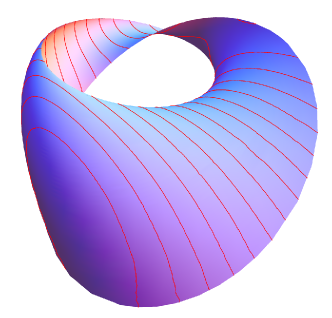
Figure 1. Stereographic projection in $\mbox{${\mathbb{R}}$}^{3}$ of the helix surface, of constant angle $\pi/4$, in $\mbox{${\mathbb{S}}$}^{3}$ given by $F$ in Example 3.3.

References

- [1] B. Daniel. Isometric immersions into -dimensional homogeneous manifolds, Comment. Math. Helv. 82, (2007), 87-131.
- [2] P. Cermelli, A. J. Di Scala. Constant-angle surfaces in liquid crystals. Phil. Mag. 87 (2007), 1871–1888.
- [3] F. Dillen, M.I. Munteanu. Constant angle surfaces in . Bull. Braz. Math. Soc. (N.S.) 40 (2009), 85–97.
- [4] F. Dillen, J. Fastenakels, J. Van der Veken, L. Vrancken. Constant angle surfaces in . Monatsh. Math. 152 (2007), 89–96.
- [5] A. Di Scala, G. Ruiz-Hernández. Higher codimensional Euclidean helix submanifolds. Kodai Math. J. 33 (2010), 192–210.
- [6] A. Di Scala, G. Ruiz-Hernández. Helix submanifolds of Euclidean spaces. Monatsh. Math. 157 (2009), 205–215.
- [7] J. Fastenakels, M.I. Munteanu, J. Van Der Veken. Constant angle surfaces in the Heisenberg group. Acta Math. Sin. (Engl. Ser.) 27 (2011), 747–756.
- [8] R. López, M.I. Munteanu. On the geometry of constant angle surfaces in . Kyushu J. Math. 65 (2011), 237–249.
- [9] D. McDuff, D. Salamon. Introduction to symplectic topology. Oxford Mathematical Monographs, Oxford University Press, New York, 1998.
- [10] G. Reeb. Sur certaines propriétés topologiques des trajectoires des systémes dynamiques. Acad. Roy. Belgique. Cl. Sci. Mém. 27 (1952).
- [11] G. Ruiz-Hernández. Minimal helix surfaces in . Abh. Math. Semin. Univ. Hambg. 81 (2011), 55–67.
- [12] F. Torralbo. Compact minimal surfaces in the Berger spheres. Indiana U. Math. J., to appear.