Electroweak form factors of heavy-light mesons –
a relativistic point-form approach

Abstract

We present a general relativistic framework for the calculation of the electroweak structure of heavy-light mesons within constituent-quark models. To this aim the physical processes in which the structure is measured, i.e. electron-meson scattering and semileptonic weak decays, are treated in a Poincaré invariant way by making use of the point-form of relativistic quantum mechanics. The electromagnetic and weak meson currents are extracted from the $1$-$\gamma$ and $1$-$W$-exchange amplitudes that result from a Bakamjian-Thomas type mass operator for the respective systems. The covariant decomposition of these currents provides the electromagnetic and weak (transition) form factors. Problems with cluster separability, which are inherent in the Bakamjian-Thomas construction, are discussed and it is shown how to keep them under control. It is proved that the heavy-quark limit of the electroweak form factors leads to one universal function, the Isgur-Wise function, confirming that the requirements of heavy-quark symmetry are satisfied. A simple analytical expression is given for the Isgur-Wise function and its agreement with a corresponding front-form calculation is verified numerically. Electromagnetic form factors for $B^{-}$ and $D^{+}$ and weak $B\rightarrow D^{(\ast)}$-decay form factors are calculated with a simple harmonic-oscilllator wave function and heavy-quark symmetry breaking due to finite masses of the heavy quarks is discussed.

I Introduction

A proper relativistic formulation of the electroweak structure of few-body bound states poses several problems. Even if one has model wave functions for the few-body bound states one is interested in, it is not straightforward to construct electromagnetic and weak currents with all the properties it should have. Two basic features are Poincaré covariance and cluster separability Sokolov (1979); Coester and Polyzou (1982); Keister and Polyzou (1991). The latter means that the bound-state current should become a sum of subsystem currents, if the interaction between the subsystems is turned off. This property is closely related to the requirement that the charge of the whole system should be the sum of the subsystem charges, irrespective whether the interaction is present or not Lev (1995). Electromagnetic currents should, furthermore, satisfy current conservation and in the case of electroweak currents of heavy-light systems one has restrictions coming from heavy-quark symmetry that should be satisfied if the mass of the heavy quark goes to infinity Isgur and Wise (1989, 1990); Neubert (1994). This is the topic which we will concentrate on in this paper keeping, of course, also the other requirements for a reasonable current in mind.

The main ingredients in the construction of currents are the wave functions of the incoming and outgoing few body bound states. Since momentum is transferred to the bound state in the course of an electroweak process, one has to know how to boost the wave function, which is usually calculated for the bound state at rest, to the initial and final state, respectively. A procedure which provides wave functions for interacting few-body systems with well defined relativistic boost properties is the, so called, Bakamjian-Thomas construction Bakamjian and Thomas (1953); Keister and Polyzou (1991). It gives an interacting representation of the Poincaré algebra on a few-body Hilbert space, allows even for instantaneous interactions, and it works in the 3 common forms of relativistic Hamiltonian dynamics Dirac (1949), the instant form, the front form and the point form. These forms are characterized by which of the Poincaré generators contain interaction terms and which are interaction free. In the point-form, which we are going to use, all 4 components of the 4-momentum operator are interaction dependent, whereas the Lorentz generators stay free of interactions. As a consequence boosts and the addition of angular momenta become simple.

There is a long list of papers in which relativistic constituent-quark models serve as a starting point for the calculation of the electroweak structure of heavy-light mesons. A lot of these calculations have been done in front form, like e.g. those in Refs.Jaus (1996); Simula (1996); Demchuk et al. (1996); Cheng et al. (1997) , to mention a few. In these papers the electromagnetic and weak meson currents are usually approximated by one-body currents, which means that those currents are assumed to be a sum of contributions in which the gauge boson couples only to one of the constituents, whereas the others act as spectators. It is well known that this approximation leads to problems with covariance of the currents in front form and in instant form Lev (1995). The form factors extracted from such a one-body approximation of a current depend, in general, on the frame in which the approximation is made. In the covariant front-form formulation suggested in Ref. Carbonell et al. (1998) this problem is circumvented by introducing additional, spurious covariants and form factors that are associated with the chosen orientation of the light front. Another way to cure this problem is the introduction of a non-valence contribution leading to a, so called, Z-graph Simula (2002); Bakker et al. (2003). Such a non-valence contribution to the currents is also included in an effective way in the instant-form approach of Ebert et al. Ebert et al. (2007). This is a very sophisticated constituent-quark model for heavy-light systems based on a quasipotential approach. A whole series of papers by Ebert and collaborators deals very comprehensively with spectroscopy, structure and decays of heavy-light mesons and baryons. In connection with instant form constituent-quark models one should also mention the papers of Le Yaouanc et al. (see, e.g., Ref. Morenas et al. (1997) and references therein). They were the first to prove that covariance of a one-body current is recovered, if the mass of the heavy quark goes to infinity Le Yaouanc et al. (1996). Thereby they made use of the known boost properties of wave functions within the Bakamjian-Thomas formulation of relativistic quantum mechanics.

On the contrary, the literature on point-form calculations of heavy-light systems is very sparse, although the point form seems to be particularly suited for the treatment of this kind of systems. We are only aware of two papers by Keister Keister (1992, 1997). This is one of our motivations to investigate the electroweak structure of heavy-light mesons within the point form of relativistic dynamics. Although it is possible to formulate a covariant one-body current in point form Klink (1998a); Melde et al. (2005), we will adopt a different strategy. Instead of making a particular ansatz for the electromagnetic and weak currents and extract the form factors from these currents, we rather want to derive these currents in such a way that they are compatible with the binding forces. The idea is to treat the physical processes in which the electroweak form factors are measured in a Poincaré invariant way by means of the Bakamjian-Thomas formalism. This gives us 1-$\gamma$ and 1-$W$-exchange amplitudes from which the currents and form factors can be extracted. This kind of procedure has already been applied successfully to the calculate electromagnetic form factors of spin-0 and spin-1 two-body bound states consisting of equal-mass particles Biernat et al. (2009); Biernat (2011). These calculations were restricted to space-like momentum transfers. For instantaneous binding forces the results were found to be equivalent with those obtained with a one-body ansatz for the current in the covariant front-form approach Carbonell et al. (1998). The present paper is an extension of the foregoing work to unequal-mass constituents and to weak decay form factors in the time-like momentum transfer region. It is also intended as a check whether the additional restrictions coming from heavy-quark symmetry can be accounted for within our approach.

The general Poincaré invariant framework that we use to describe electron-meson scattering and semileptonic weak decays of mesons will be introduced in Sec. II. It is a relativistic multichannel formalism for a Bakamjian-Thomas type mass operator Bakamjian and Thomas (1953); Keister and Polyzou (1991) that is represented in a velocity-state basis Klink (1998a). This multichannel formulation is necessary to account for the dynamics of $\gamma$- and $W$-exchange, respectively. The one-photon-exchange amplitude for electron scattering off a confined quark-antiquark pair is derived in Sec. II.2, the one-$W$-exchange amplitude for the semileptonic decay of a confined quark-antiquark state into another (confined) quark-antiquark state in Sec. II.3. Since these amplitudes have the usual structure, namely lepton current contracted with hadron current times gauge-boson propagator, it is easy to identify the electromagnetic and weak hadron currents. This is explicitly done for pseudoscalar mesons and pseodscalar-to-pseudoscalar as well as pseudoscalar-to-vector transitions assuming that the mesons are pure $s$-wave. The Lorentz-structure of the resulting electromagnetic and weak currents is then analyzed in Sec. III. As a result of this analysis we obtain the electroweak form factors. Section III.1 contains also a short discussion of cluster problems, connected with the Bakamjian-Thomas construction, and their effect on the electromagnetic current. The limit of heavy-quark mass going to infinity is investigated in Sec. IV. The precise definition of the “heavy-quark limit” is introduced and it is proved that the heavy-quark limit of the electromagnetic and weak from factors yields a single universal function, the Isgur-Wise function. Model calculations of the electromagnetic $D^{+}$ and $B^{-}$ form factors and weak $B\rightarrow D^{(\ast)}$ decay form factors for physical masses of the heavy quarks are presented in Sec. V. These are contrasted with the Isgur-Wise function to estimate heavy-quark-symmetry breaking effects due to finite masses of the heavy quarks. Our summary and conclusions are finally given in Sec. VI.

II Coupled-channel formalism

II.1 Prerequisites

In the point-form version of the Bakamjian-Thomas construction the 4-momentum operator for an interacting few-body system is written as a product of an interaction-dependent mass operator times a free 4-velocity operator Keister and Polyzou (1991),

$$\hat{P}^{\mu}=\hat{M}\,\hat{V}^{\mu}_{\mathrm{free}}=(\hat{M}_{\mathrm{free}}+\hat{M}_{\mathrm{int}})\,\hat{V}^{\mu}_{\mathrm{free}}\,.$$ (1)

Relativistic invariance holds if the interaction term $\hat{M}_{\mathrm{int}}$ is a Lorentz scalar and commutes with $\hat{V}^{\mu}_{\mathrm{free}}$. Equation (1) implies that the overall velocity of the system can be easily separated from the internal motion and one can concentrate on studying the mass operator $\hat{M}$ which is a function of the internal variables only.

In this type of approach the operators of interest are most conveniently represented in a velocity-state basis Klink (1998b). An $n$-particle velocity state $|v;\vec{k}_{1},\mu_{1};\vec{k}_{2},\mu_{2};\dots;\vec{k}_{n},\mu_{n}\rangle$ is just a multiparticle momentum state in the rest frame that is boosted to overall 4-velocity $v$ ($v_{\mu}v^{\mu}=1$) by means of a canonical spin boost $B_{c}(v)$ Keister and Polyzou (1991):

$$|v;\vec{k}_{1},\mu_{1};\vec{k}_{2},\mu_{2};\dots;\vec{k}_{n},\mu_{n}\rangle$$

$$:=\hat{U}_{B_{c}(v)}\,|\vec{k}_{1},\mu_{1};\vec{k}_{2},\mu_{2};\dots;\vec{k}_{n},\mu_{n}\rangle\,\,\mathrm{with}\,\,\sum_{i=1}^{n}\vec{k}_{i}=0\,.$$

The $\mu_{i}$s are the spin projections of the individual particles. By construction one of the $\vec{k}_{i}$s is redundant. Velocity states are orthogonal

$$\!\!\!\!\!\!\!\!\!\langle v^{\prime};\vec{k}_{1}^{\prime},\mu_{1}^{\prime};\vec{k}_{2}^{\prime},\mu_{2}^{\prime};\dots;\vec{k}_{n}^{\prime},\mu_{n}^{\prime}|\,v;\vec{k}_{1},\mu_{1};\vec{k}_{2},\mu_{2};\dots;\vec{k}_{n},\mu_{n}\rangle$$ (3)

$$=v_{0}\,\delta^{3}(\vec{v}^{\prime}-\vec{v})\,\frac{(2\pi)^{3}2\omega_{k_{n}}}{\left(\sum_{i=1}^{n}\omega_{k_{i}}\right)^{3}}$$

$$\phantom{=}\times\left(\prod_{i=1}^{n-1}(2\pi)^{3}2\omega_{k_{i}}\delta^{3}(\vec{k}_{i}^{\prime}-\vec{k}_{i})\right)\left(\prod_{i=1}^{n}\delta_{\mu_{i}^{\prime}\mu_{i}}\right)\,$$

and satisfy the completeness relation

$$\mathds{1}_{1,2,\dots,n} = \sum_{\mu_{1}=-j_{1}}^{j_{1}}\sum_{\mu_{2}=-j_{2}}^{j_{2}}\dots\sum_{\mu_{n}=-j_{n}}^{j_{n}}\int\frac{d^{3}v}{(2\pi)^{3}v_{0}}$$ (4)

$$\times\left[\prod_{i=1}^{n-1}\frac{d^{3}k_{i}}{(2\pi)^{3}2\omega_{k_{i}}}\right]\frac{\left(\sum_{i=1}^{n}\omega_{k_{i}}\right)^{3}}{2\omega_{k_{n}}}$$

$$\times|v;\vec{k}_{1},\mu_{1};\vec{k}_{2},\mu_{2};\dots;\vec{k}_{n},\mu_{n}\rangle$$

$$\times\langle v;\vec{k}_{1},\mu_{1};\vec{k}_{2},\mu_{2};\dots;\vec{k}_{n},\mu_{n}|\,,$$

with $m_{i}$, $\omega_{k_{i}}:=\sqrt{m_{i}^{2}+\vec{k}_{i}^{2}}$, and $j_{i}$, being the mass, the energy, and the spin of the $i$th particle, respectively. Without loss of generality we have taken the $n$th momentum to be redundant.

One of the big advantages of velocity states as compared with usual momentum states is their simple behavior under a Lorentz transformation $\Lambda$:

$$\hat{U}_{\Lambda}|v;\vec{k}_{1},\mu_{1};\vec{k}_{2},\mu_{2};\dots;\vec{k}_{n},\mu_{n}\rangle$$ (5)

$$=\sum_{\mu_{1}^{\prime},\mu_{2}^{\prime},\dots,\mu_{n}^{\prime}}\,\left\{\prod_{i=1}^{n}\,D^{j_{i}}_{\mu_{i}^{\prime}\mu_{i}}\left[R_{\mathrm{W}}(v,\Lambda)\right]\right\}|\Lambda v;\overrightarrow{R_{\mathrm{W}}(v,\Lambda)k}_{1},\mu_{1}^{\prime};\overrightarrow{R_{\mathrm{W}}(v,\Lambda)k}_{2},\mu_{2}^{\prime};\dots;\overrightarrow{R_{\mathrm{W}}(v,\Lambda)k}_{n},\mu_{n}^{\prime}\rangle\,,$$

with the Wigner-rotation matrix

$$R_{\mathrm{W}}(v,\Lambda)=B_{c}^{-1}(\Lambda v)\Lambda B_{c}(v)\,.$$ (6)

Since the Wigner rotations are the same for all particles angular momenta can be added as in non-relativistic quantum mechanics. In a velocity-state basis the Bakamjian-Thomas type 4-momentum operator, Eq. (1), is diagonal in the 4-velocity $v$.

II.2 Electron-meson scattering

We extract the electromagnetic meson current and the corresponding form factors from the invariant one-photon-exchange amplitude for electron-meson scattering. This requires to take the dynamics of the exchanged photon fully into account. Hence we formulate the scattering of an electron by a (composite) meson on a Hilbert space that is a direct sum of $eQ\bar{q}$ and $eQ\bar{q}\gamma$ Hilbert spaces. If the eigenstates $|\psi\rangle$ of the total mass operator $\hat{M}$ are decomposed into $eQ\bar{q}$ and $eQ\bar{q}\gamma$ components, i.e. $|\psi\rangle=|\psi_{eQ\bar{q}}\rangle+|\psi_{eQ\bar{q}\gamma}\rangle$, the mass-eigenvalue equations for these components may be written in the form:

$$\left(\begin{array}[]{cc}\hat{M}^{\mathrm{conf}}_{eQ\bar{q}}&\hat{K}_{\gamma}\\ \hat{K}_{\gamma}^{\dagger}&\hat{M}^{\mathrm{conf}}_{eQ\bar{q}\gamma}\end{array}\right)\left(\begin{array}[]{l}|\psi_{eQ\bar{q}}\rangle\\ |\psi_{eQ\bar{q}\gamma}\rangle\end{array}\right)=m\left(\begin{array}[]{l}|\psi_{eQ\bar{q}}\rangle\\ |\psi_{eQ\bar{q}\gamma}\rangle\end{array}\right)\,.$$ (13)

$\hat{K}_{\gamma}^{\dagger}$ and $\hat{K}_{\gamma}$ are vertex operators that describe the emission and absorption of a photon by the electron or (anti)quark. Without loss of generality we have assumed that the quark $Q$ ($=c,b$) is the heavy and the antiquark $\bar{q}$ ($=\bar{u},\bar{d},\bar{s}$) the light mesonic constituent, respectively. The instantaneous confining interaction between quark and antiquark is already included in the diagonal elements of this matrix mass operator, i.e.

$$\hat{M}^{\mathrm{conf}}_{eQ\bar{q}}=\hat{M}_{eQ\bar{q}}+\hat{V}^{(3)}_{\mathrm{conf}}\,,$$

$$\hat{M}^{\mathrm{conf}}_{eQ\bar{q}\gamma}=\hat{M}_{eQ\bar{q}\gamma}+\hat{V}^{(4)}_{\mathrm{conf}}\,,$$ (14)

with $\hat{V}^{(3)}_{\mathrm{conf}}$ and $\hat{V}^{(4)}_{\mathrm{conf}}$ denoting the embedding of the confining $Q\bar{q}$-potential into the 3- and 4-particle Hilbert spaces Keister and Polyzou (1991).

The invariant one-photon exchange amplitude for electron-meson scattering is now obtained by taking appropriate matrix elements of the optical potential $\hat{V}_{\mathrm{opt}}(m)$ that enters the equation for $|\psi_{eQ\bar{q}}\rangle$ after a Feshbach reduction:

$$(\hat{M}^{\mathrm{conf}}_{eQ\bar{q}}+\underbrace{\hat{K}_{\gamma}(m-\hat{M}^{\mathrm{conf}}_{eQ\bar{q}\gamma})^{-1}\hat{K}_{\gamma}^{\dagger}}_{\hat{V}_{\mathrm{opt}}(m)})|\psi_{eQ\bar{q}}\rangle=|\psi_{eQ\bar{q}}\rangle\,.$$ (15)

What we need are matrix elements of the optical potential $\hat{V}_{\mathrm{opt}}(m)$ between (velocity) eigenstates of the channel mass operator

$$M^{\mathrm{conf}}_{eQ\bar{q}}|\,\underline{v};\vec{\underline{k}}_{e},\underline{\mu}_{e};\vec{\underline{k}}_{\alpha},\underline{\mu}_{\alpha},\alpha\rangle$$ (16)

$$\qquad=(\omega_{\underline{k}_{e}}+\omega_{\underline{k}_{\alpha}})|\,\underline{v};\vec{\underline{k}}_{e},\underline{\mu}_{e};\vec{\underline{k}}_{\alpha},\underline{\mu}_{\alpha},\alpha\rangle\,.$$

$\underline{\mu}_{\alpha}$ denotes the spin orientation of the confined $q\bar{q}$ bound state, $\alpha$ is a shorthand notation for the remaining discrete quantum numbers necessary to specify it uniquely. The energy of the $Q\bar{q}$ bound state with quantum numbers $\alpha$ and mass $m_{\alpha}$ is $\omega_{\underline{k}_{\alpha}}=(m_{\alpha}^{2}+\vec{\underline{k}}_{\alpha}^{2})^{1/2}$. Eigenstates of $M^{\mathrm{conf}}_{eQ\bar{q}\gamma}$ are introduced in an analogous way. Later on we will also need (velocity) eigenstates of the free mass operators $M_{eQ\bar{q}}$ and $M_{eQ\bar{q}\gamma}$. To make a clear distinction between states with a confined $Q\bar{q}$ pair from those with a free $Q\bar{q}$ pair we underline velocities, momenta and spin projections for the former. For the calculation of electromagnetic meson form factors only on-shell matrix elements of $\hat{V}_{\mathrm{opt}}(m)$ are required with the discrete quantum numbers $\alpha$ being those of the meson of interest. The further analysis of these on-shell matrix elements is accomplished by inserting completeness relations for the eigenstates of $M^{\mathrm{conf}}_{eQ\bar{q}\gamma}$, $M_{eQ\bar{q}}$ and $M_{eQ\bar{q}\gamma}$ at the appropriate places:

$$\langle\underline{v}^{\prime};\vec{\underline{k}}_{e}^{\prime},\underline{\mu}_{e}^{\prime};\vec{\underline{k}}_{\alpha}^{\prime},\underline{\mu}_{\alpha}^{\prime},\alpha|\,\hat{V}_{\mathrm{opt}}(m)|\,\underline{v};\vec{\underline{k}}_{e},\underline{\mu}_{e};\vec{\underline{k}}_{\alpha},\underline{\mu}_{\alpha},\alpha\rangle_{\mathrm{os}}$$

$$=\langle\underline{v}^{\prime};\vec{\underline{k}}_{e}^{\prime},\underline{\mu}_{e}^{\prime};\vec{\underline{k}}_{\alpha}^{\prime},\underline{\mu}_{\alpha}^{\prime},\alpha|\,\mathds{1}_{eQ\bar{q}}\,\hat{K}_{\gamma}\mathds{1}_{eQ\bar{q}\gamma}\left(\hat{M}_{eQ\bar{q}\gamma}^{\text{conf}}\!-\!m\right)^{-1}$$

$$\quad\times\mathds{1}_{eQ\bar{q}\gamma}^{\mathrm{conf}}\mathds{1}_{eQ\bar{q}\gamma}\,\hat{K}^{\dagger}_{\gamma}\mathds{1}_{eQ\bar{q}}\,|\,\underline{v};\vec{\underline{k}}_{e},\underline{\mu}_{e};\vec{\underline{k}}_{\alpha},\underline{\mu}_{\alpha},\alpha\rangle_{\mathrm{os}}\,.$$

“os” means on-shell, i.e. $m=\omega_{\underline{k}_{e}}+\omega_{\underline{k}_{\alpha}}=\omega_{\underline{k}_{e}^{\prime}}+\omega_{\underline{k}_{\alpha}^{\prime}}$, $\omega_{\underline{k}_{e}}=\omega_{\underline{k}_{e}^{\prime}}$ and $\omega_{\underline{k}_{\alpha}}=\omega_{\underline{k}_{\alpha}^{\prime}}$. After insertion of the completeness relations one ends up with matrix elements of the form $\langle v;\vec{k}_{e},\mu_{e};\vec{k}_{Q},\mu_{Q};\vec{k}_{\bar{q}},\mu_{\bar{q}}|\,\underline{v};\vec{\underline{k}}_{e},\underline{\mu}_{e};\vec{\underline{k}}_{\alpha},\underline{\mu}_{\alpha},\alpha\rangle$, $\langle v;\vec{k}_{e},\mu_{e};\vec{k}_{Q},\mu_{Q};\vec{k}_{\bar{q}},\mu_{\bar{q}};\vec{k}_{\gamma},\mu_{\gamma}|\,\underline{v};\vec{\underline{k}}_{e},\underline{\mu}_{e};\vec{\underline{k}}_{\alpha},\underline{\mu}_{\alpha},\alpha;\vec{\underline{k}}_{\gamma},\underline{\mu}_{\gamma}\rangle$, $\langle v^{\prime};\vec{k}_{e}^{\prime},\!\mu_{e}^{\prime};\vec{k}_{Q}^{\prime},\!\mu_{Q}^{\prime};\vec{k}_{\bar{q}}^{\prime},\!\mu_{\bar{q}}^{\prime};\vec{k}_{\gamma}^{\prime},\!\mu_{\gamma}^{\prime}|\,\hat{K}^{\dagger}\,|v\,;\vec{k}_{e},\!\mu_{e};\vec{k}_{Q},\!\mu_{Q};\vec{k}_{\bar{q}},\!\mu_{\bar{q}}\rangle$ and the Hermitian conjugates, respectively. The first two are just wave functions of the confined $Q\bar{q}$ pair and a free electron (and photon). The third describes the transition from a free $Q\bar{q}e$ state to a free $Q\bar{q}e\gamma$ state by emission of a photon and is calculated from the usual interaction density ${\mathcal{L}}^{\mathrm{em}}_{\mathrm{int}}(x)$ of spinor quantum electrodynamics Klink (2003):

$$\langle v^{\prime};\vec{k}_{e}^{\prime},\!\mu_{e}^{\prime};\vec{k}_{Q}^{\prime},\!\mu_{Q}^{\prime};\vec{k}_{\bar{q}}^{\prime},\!\mu_{\bar{q}}^{\prime};\vec{k}_{\gamma}^{\prime},\!\mu_{\gamma}^{\prime}|\,\hat{K}^{\dagger}\,|v\,;\vec{k}_{e},\!\mu_{e};\vec{k}_{Q},\!\mu_{Q};\vec{k}_{\bar{q}},\!\mu_{\bar{q}}\rangle$$ (18)

$$= Nv_{0}\delta^{3}(\vec{v}^{\prime}-\vec{v})\,\langle\vec{k}_{e}^{\prime},\!\mu_{e}^{\prime};\vec{k}_{Q}^{\prime},\!\mu_{Q}^{\prime};\vec{k}_{\bar{q}}^{\prime},\!\mu_{\bar{q}}^{\prime};\vec{k}_{\gamma}^{\prime},\!\mu_{\gamma}^{\prime}|$$

$$\times\hat{\mathcal{L}}^{\mathrm{em}}_{\mathrm{int}}(0)\,|\vec{k}_{e},\!\mu_{e};\vec{k}_{Q},\!\mu_{Q};\vec{k}_{\bar{q}},\!\mu_{\bar{q}}\rangle\,.$$

The normalization factor $N$ is determined by the normalization of the velocity states. Explicit expressions for all the matrix elements are given in Ref. Biernat et al. (2009). Using these analytical results we can show that the on-shell matrix elements of the optical potential have the structure that one expects from the invariant one-photon-exchange amplitude, namely the electron current $j_{e}^{\mu}$ contracted with the hadron current $\tilde{J}^{\nu}_{[\alpha]}$ and multiplied with the covariant photon propagator $(-g_{\mu\nu}/Q^{2})$ (times some kinematical factors):

$$\langle\underline{v}^{\prime};\vec{\underline{k}}_{e}^{\prime},\underline{\mu}_{e}^{\prime};\vec{\underline{k}}_{\alpha}^{\prime},\underline{\mu}_{\alpha}^{\prime},\alpha|\,\hat{V}_{\mathrm{opt}}(m)|\,\underline{v};\vec{\underline{k}}_{e},\underline{\mu}_{e};\vec{\underline{k}}_{\alpha},\underline{\mu}_{\alpha}^{\prime},\alpha\rangle_{\mathrm{os}}$$ (19)

$$=\underline{v}_{0}\delta^{3}(\vec{\underline{v}}^{\,\prime}-\vec{\underline{v}}\,)\,\frac{(2\pi)^{3}}{\sqrt{(\omega_{\underline{k}_{e}^{\prime}}+\omega_{\underline{k}_{\alpha}^{\prime}})^{3}}\sqrt{(\omega_{\underline{k}_{e}^{\phantom{\prime}}}+\omega_{\underline{k}_{\alpha}^{\phantom{\prime}}})^{3}}}(-e^{2})\underbrace{\,\bar{u}_{\underline{\mu}_{e}^{\prime}}(\vec{\underline{k}}_{e}^{\prime})\gamma^{\mu}u_{\underline{\mu}_{e}}(\vec{\underline{k}}_{e})}_{j_{e}^{\mu}(\vec{\underline{k}}_{e}^{\prime},\underline{\mu}_{e}^{\prime};\vec{\underline{k}}_{e},\underline{\mu}_{e})}\frac{(-g_{\mu\nu})}{Q^{2}}\underbrace{(Q_{Q}J_{Q}^{\nu}(\dots)+Q_{\bar{q}}J_{\bar{q}}^{\nu}(\dots))}_{\tilde{J}_{[\alpha]}^{\nu}(\vec{\underline{k}}_{\alpha}^{\prime},\underline{\mu}_{\alpha}^{\prime};\vec{\underline{k}}_{\alpha},\underline{\mu}_{\alpha})}\,.$$

Here we have introduced the (negative) square of the (space-like) 4-momentum-transfer $Q^{2}=-\underline{q}_{\mu}\underline{q}^{\mu}$, with $\underline{q}^{\mu}=(\underline{k}_{\alpha}-\underline{k}_{\alpha}^{\prime})^{\mu}=(\underline{k}_{e}^{\prime}-\underline{k}_{e})^{\mu}$. $e$, $Q_{Q}|\,e|$ and $Q_{\bar{q}}|\,e|$ denote the electric charges of the electron, the quark and the antiquark, respectively. We want to emphasize that the kinematical factor in front of Eq. (19) and thus the normalization of the meson current $\tilde{J}^{\nu}_{[\alpha]}$ is uniquely fixed. It must be identical with the one that comes out if the optical potential is derived in an analogous way for the scattering of an electron by a point-like meson with discrete quantum numbers $\alpha$ (see Refs. Biernat et al. (2009); Biernat (2011)). Since the point-like current is known this kinematical factor can be uniquely identified. The two parts of the meson current, $J_{Q}^{\nu}$ and $J_{\bar{q}}^{\nu}$, correspond to the coupling of the photon to the quark or the antiquark, respectively. If $\alpha$ are the discrete quantum numbers of a pseudoscalar ground-state meson ($\underline{\mu}_{\alpha}=\underline{\mu}_{\alpha}^{\prime}=0$) it has to be a pure s-wave and we find that

$$J^{\nu}_{Q}(\vec{\underline{k}}_{\alpha}^{\prime},\vec{\underline{k}}_{\alpha})=\frac{\sqrt{\omega_{\underline{k}_{\alpha}}\omega_{\underline{k}_{\alpha}^{\prime}}}}{4\pi}\int\,\frac{d^{3}\tilde{k}_{\bar{q}}^{\prime}}{2\omega_{k_{Q}}}\,\sqrt{\frac{\omega_{{k}_{Q}}+\omega_{{k}_{\bar{q}}}}{\omega_{{k}^{\prime}_{Q}}+\omega_{{k}^{\prime}_{\bar{q}}}}}\,\sqrt{\frac{\omega_{\tilde{k}^{\prime}_{Q}}+\omega_{\tilde{k}^{\prime}_{\bar{q}}}}{\omega_{\tilde{k}_{Q}}+\omega_{\tilde{k}_{\bar{q}}}}}\,\sqrt{\frac{\omega_{\tilde{k}_{Q}}\omega_{\tilde{k}_{\bar{q}}}}{\omega_{\tilde{k}^{\prime}_{Q}}\omega_{\tilde{k}^{\prime}_{\bar{q}}}}}\,\bigg{\{}\!\sum_{\mu_{Q},\mu_{Q}^{\prime}=\pm\frac{1}{2}}\!\!\!\bar{u}_{\mu_{Q}^{\prime}}(\vec{k}_{Q}^{\prime})\,\gamma^{\nu}\,u_{\mu_{Q}}(\vec{k}_{Q})$$ (20)

$$\times D^{1/2}_{\mu_{Q}\mu_{Q}^{\prime}}\!\left[\!R_{\mathrm{W}}\!\left(\frac{\tilde{k}_{Q}}{m_{Q}},B_{c}(v_{Q\bar{q}})\right)\,\!R^{-1}_{\mathrm{W}}\!\left(\frac{\tilde{k}_{\bar{q}}}{m_{\bar{q}}},B_{c}(v_{Q\bar{q}})\right)\,\!R_{\mathrm{W}}\!\left(\frac{\tilde{k}_{\bar{q}}^{\prime}}{m_{\bar{q}}},B_{c}(v_{Q\bar{q}}^{\prime})\right)\,\!R^{-1}_{\mathrm{W}}\!\left(\frac{\tilde{k}_{Q}^{\prime}}{m_{Q}},B_{c}(v_{Q\bar{q}}^{\prime})\right)\right]\bigg{\}}\,\psi^{\ast}\,(|\vec{\tilde{k}}_{\bar{q}}^{\prime}|)\,\psi\,(|\vec{\tilde{k}}_{\bar{q}}|)\,\,.$$

The corresponding expression for $J^{\nu}_{\bar{q}}$ is obtained by interchanging $Q$ and $\bar{q}$ in Eq. (20). The quantities with a tilde are defined in the rest frame of the $Q\bar{q}$ subsystem. The s-wave bound-state wave function $\psi(\kappa)$ is also defined in this frame and normalized according to

$$\int_{0}^{\infty}\,d\kappa\kappa^{2}\,\psi^{\ast}(\kappa)\,\psi(\kappa)=1\,.$$ (21)

The transformation between the $Q\bar{q}$ rest frame and the $Q\bar{q}e$ rest frame is accomplished by means of a canonical spin boost Keister and Polyzou (1991)

$$B_{c}(v)=\left(\begin{array}[]{cc}v^{0}&\mathbf{v}^{T}\\ \mathbf{v}&\mathbf{1}+\frac{v^{0}-1}{\mathbf{v}^{2}}\mathbf{v}\mathbf{v}^{T}\end{array}\right)$$ (22)

with

$$v=v_{Q\bar{q}}=\frac{k_{Q}+k_{\bar{q}}}{m_{Q\bar{q}}}$$ (23)

and

$$m_{Q\bar{q}}=\omega_{\tilde{k}_{Q}}+\omega_{\tilde{k}_{\bar{q}}}=\sqrt{(\omega_{k_{Q}}+\omega_{k_{\bar{q}}})^{2}-(\vec{k}_{Q}+\vec{k}_{\bar{q}})^{2}}\,$$ (24)

denoting the invariant mass of the (unbound) $Q\bar{q}$ pair. Here it is useful to note that, due to our center-of-mass kinematics, $\vec{k}_{e}+\vec{k}_{Q}+\vec{k}_{\bar{q}}=\vec{k}_{e}+\vec{\underline{k}}_{\alpha}=0$ and hence $\vec{k}_{Q}+\vec{k}_{\bar{q}}=\vec{\underline{k}}_{\alpha}$ such that $\vec{v}_{Q\bar{q}}=\vec{\underline{k}}_{\alpha}/m_{Q\bar{q}}$. Analogous relations hold for $v_{Q\bar{q}}^{\prime}$ and the primed momenta. This implies further that not all of the 4-momentum that is transferred via the photon to the $Q\bar{q}$ bound state is also transferred to the active constituent. Only the 3-momentum transfer is the same. For the quark being the active particle we have, e.g., $\vec{\underline{q}}=\vec{\underline{k}}_{\alpha}-\vec{\underline{k}}_{\alpha}^{\prime}=\vec{k}_{Q}-\vec{k}_{Q}^{\prime}=:\vec{q}_{\mathrm{quark}}$. On the other hand one has $\omega_{\underline{k}_{\alpha}}=\omega_{\underline{k}_{\alpha}^{\prime}}$ and hence $\underline{q}^{0}=0$, whereas, in general, $q^{0}_{\mathrm{quark}}:=\omega_{k_{Q}}-\omega_{k_{Q}^{\prime}}\neq 0$. If the photon couples to the quark, the spectator condition $k_{\bar{q}}=k_{\bar{q}}^{\prime}$ for the antiquark implies the relation:

$$\tilde{k}_{\bar{q}} = B_{c}^{-1}(v_{Q\bar{q}})\,k_{\bar{q}}=B_{c}^{-1}(v_{Q\bar{q}})\,k_{\bar{q}}^{\prime}$$ (25)

$$= B_{c}^{-1}(v_{Q\bar{q}})\,B_{c}(v_{Q\bar{q}}^{\prime})\tilde{k}_{\bar{q}}^{\prime}\,.$$

The 4-momenta $\tilde{k}_{Q}^{(\prime)}$ for the active quark are then uniquely determined by $\vec{\tilde{k}}_{Q}^{(\prime)}=-\vec{\tilde{k}}_{\bar{q}}^{(\prime)}$. Associated with the boosts that connect incoming and outgoing wave functions are Wigner rotations of the quark and antiquark spins. The corresponding Wigner $D$ functions can be combined to the single one showing up in Eq. (20) by means of the spectator conditions and the Clebsch coefficients that couple the quark and the antiquark spins to zero meson spin (see, e.g., Ref. Biernat (2011)).

Having obtained the microscopic expression for the electromagnetic meson current $\tilde{J}^{\nu}_{[\alpha]}$ (cf. Eqs. (19) and (20)), we will show in the sequel how the derivation of the weak current, as occurring in semileptonic meson decays, is accomplished within our relativistic coupled-channel framework.

II.3 Semileptonic meson decay

In order to get the full (leading-order) invariant amplitude for the semileptonic weak decay of a heavy-light meson $\alpha$ into another heavy-light meson $\alpha^{\prime}$ one needs at least 4 channels. This can be seen immediately, if one decomposes this amplitude into its time-ordered contributions. This decomposition is depicted in Fig. 1 for the $\bar{B}^{0}\rightarrow D^{(\ast)+}e\bar{\nu}_{e}$ decay on which we will concentrate in the following. In addition to the incoming $b\bar{d}$ channel and the outgoing $c\bar{d}e\bar{\nu}_{e}$ channel one needs a $c\bar{d}W$ and a $b\bar{d}We\bar{\nu}_{e}$ channel to account for the intermediate states in which the $W$-boson is in flight. The matrix mass operator acting on all these channels has the form

$$\left(\begin{array}[]{cccc}\hat{M}^{\mathrm{conf}}_{b\bar{d}}&0&\hat{K}_{c\bar{d}W\rightarrow b\bar{d}}&\hat{K}_{b\bar{d}We\bar{\nu}_{e}\rightarrow b\bar{d}}\\ 0&\hat{M}^{\mathrm{conf}}_{c\bar{d}e\bar{\nu}_{e}}&\hat{K}_{c\bar{d}W\rightarrow c\bar{d}e\bar{\nu}_{e}}&\hat{K}_{b\bar{d}We\bar{\nu}_{e}\rightarrow c\bar{d}e\bar{\nu}_{e}}\\ \hat{K}^{\dagger}_{c\bar{d}W\rightarrow b\bar{d}}&\hat{K}^{\dagger}_{c\bar{d}W\rightarrow c\bar{d}e\bar{\nu}_{e}}&\hat{M}^{\mathrm{conf}}_{c\bar{d}W}&0\\ \hat{K}^{\dagger}_{b\bar{d}We\bar{\nu}_{e}\rightarrow b\bar{d}}&\hat{K}^{\dagger}_{b\bar{d}We\bar{\nu}_{e}\rightarrow c\bar{d}e\bar{\nu}_{e}}&0&\hat{M}^{\mathrm{conf}}_{b\bar{d}We\bar{\nu}_{e}}\end{array}\right)\,.$$ (26)

As in the electromagnetic case an instantaneous confining potential between the quark-antiquark pair is included in the channel mass operators on the diagonal. What we are interested in is the transition from the $b\bar{d}$ to the $c\bar{d}e\bar{\nu}_{e}$ channel. As can be seen from Eq. (26) this cannot happen directly. It only works via the intermediate states that contain the $W$. The corresponding (optical) transition potential $\hat{V}_{\mathrm{opt}}^{b\bar{d}\rightarrow c\bar{d}e\bar{\nu}_{e}}(m)$ may be again obtained by applying a Feshbach reduction to eliminate the $c\bar{d}W$ and the $b\bar{d}We\bar{\nu}_{e}$ channels such that one ends up with a mass eigenvalue problem for the (coupled) $b\bar{d}$ and $c\bar{d}e\bar{\nu}_{e}$ system. The transition potential has then the form

$$\hat{V}_{\mathrm{opt}}^{b\bar{d}\rightarrow c\bar{d}e\bar{\nu}_{e}}(m)=\hat{K}_{c\bar{d}W\rightarrow c\bar{d}e\bar{\nu}_{e}}(m-M^{\mathrm{conf}}_{c\bar{d}W})^{-1}\hat{K}^{\dagger}_{c\bar{d}W\rightarrow b\bar{d}}+\hat{K}_{b\bar{d}We\bar{\nu}_{e}\rightarrow c\bar{d}e\bar{\nu}_{e}}(m-\hat{M}^{\mathrm{conf}}_{b\bar{d}We\bar{\nu}_{e}})^{-1}\hat{K}^{\dagger}_{b\bar{d}We\bar{\nu}_{e}\rightarrow b\bar{d}}\,.$$ (27)

The two terms on the right-hand side correspond to the two time-orderings of the $W$ exchange that are depicted in Fig. 1.

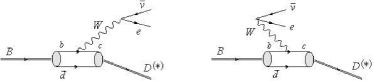
Figure 1: The two time ordered contributions to the semileptonic weak decay of a $\bar{B}^{0}$ into a $D^{(\ast)+}$ meson.

Like in the electromagnetic case the weak hadronic current and the $B\rightarrow D^{(\ast)}$ decay form factors are extracted from on-shell matrix elements of $\hat{V}_{\mathrm{opt}}^{b\bar{d}\rightarrow c\bar{d}e\bar{\nu}_{e}}(m)$, i.e. from

$$\langle\underline{v}^{\prime};\vec{\underline{k}}_{e}^{\prime},\underline{\mu}_{e}^{\prime};\vec{\underline{k}}_{\bar{\nu}_{e}}^{\prime};\vec{\underline{k}}_{\alpha^{\prime}}^{\prime},\underline{\mu}_{\alpha^{\prime}}^{\prime},\alpha^{\prime}|\hat{V}_{\mathrm{opt}}^{b\bar{d}\rightarrow c\bar{d}e\bar{\nu}_{e}}(m)|\vec{\underline{k}}_{\alpha},\underline{\mu}_{\alpha},\alpha\rangle_{\mathrm{os}}\,,$$ (28)

where the discrete quantum numbers $\alpha$ and $\alpha^{\prime}$ of the confined heavy-light system are those of the $B$ and $D^{(\ast)}$, respectively. “On shell”means now that $m=m_{B}=\omega_{\underline{k}_{\alpha}}=\omega_{\underline{k}_{\alpha^{\prime}}^{\prime}}+\omega_{\underline{k}_{e}^{\prime}}+\omega_{\underline{k}_{\bar{\nu}_{e}}^{\prime}}$. For the analysis of these matrix elements we can proceed as in the electromagnetic case. One has to insert the appropriate completeness relations at the pertinent places. This leads again to wave functions for the confined $Q^{(\prime)}\bar{q}$ pair in combination with a free $W$ and/or a free $e$-$\bar{\nu}_{e}$ pair. The matrix elements of the weak vertex operators $\hat{K}_{c\bar{d}W\rightarrow b\bar{d}}$, etc., can be derived from the weak interaction density $\mathcal{L}^{\mathrm{wk}}_{\mathrm{int}}(x)$ in analogy to Eq. (18). After insertion of the analytical expressions for the wave functions and the vertex matrix elements into Eq. (28) we observe again that the on-shell matrix elements of $V_{\mathrm{opt}}^{b\bar{d}\rightarrow c\bar{d}e\bar{\nu}_{e}}(m)$ have the same structure as the invariant $B\rightarrow D^{(\ast)}e\bar{\nu}_{e}$ decay amplitude that results from leading-order covariant perturbation theory:

$$\langle\underline{v}^{\prime};\vec{\underline{k}}_{e}^{\prime},\underline{\mu}_{e}^{\prime};\vec{\underline{k}}_{\bar{\nu}_{e}}^{\prime};\vec{\underline{k}}_{\alpha^{\prime}}^{\prime},\underline{\mu}_{\alpha^{\prime}}^{\prime},\alpha^{\prime}|\hat{V}_{\mathrm{opt}}^{b\bar{d}\rightarrow c\bar{d}e\bar{\nu}_{e}}(m)|\vec{\underline{k}}_{\alpha},\underline{\mu}_{\alpha},\alpha\rangle_{\mathrm{os}}$$

$$= \underline{v}_{0}\delta^{3}(\vec{\underline{v}}^{\,\prime}-\vec{\underline{v}}\,)\,\frac{(2\pi)^{3}}{\sqrt{(\omega_{\underline{k}_{e}^{\prime}}+\omega_{\underline{k}_{\bar{\nu}_{e}}^{\prime}}+\omega_{\underline{k}_{\alpha^{\prime}}^{\prime}})^{3}}\sqrt{\omega_{\underline{k}_{\alpha}^{\phantom{\prime}}}^{3}}}$$

$$\times\frac{e^{2}}{2\sin^{2}\vartheta_{\mathrm{w}}}V_{cb}\,\frac{1}{2}\underbrace{\bar{u}_{\underline{\mu}_{e}^{\prime}}(\vec{\underline{k}}_{e}^{\prime})\gamma^{\mu}(1-\gamma^{5})v_{\underline{\mu}_{\bar{\nu}_{e}}^{\prime}}(\vec{\underline{k}}_{\bar{\nu}_{e}}^{\prime})}_{j_{\nu_{e}\rightarrow e}^{\mu}(\vec{\underline{k}}_{e}^{\prime},\underline{\mu}_{e}^{\prime};\vec{\underline{k}}_{\bar{\nu}_{e}}^{\prime},\underline{\mu}_{\bar{\nu}_{e}}^{\prime})}$$

$$\times\frac{(-g_{\mu\nu})}{(\underline{k}^{\prime}_{e}+\underline{k}^{\prime}_{\bar{\nu}_{e}})^{2}-m_{W}^{2}}\frac{1}{2}{J_{\alpha\rightarrow\alpha^{\prime}}^{\nu}(\vec{\underline{k}}_{\alpha^{\prime}}^{\prime},\underline{\mu}_{\alpha^{\prime}}^{\prime};\vec{\underline{k}}_{\alpha},\underline{\mu}_{\alpha})}\,.$$

Here $\vartheta_{\mathrm{w}}$ denotes the electroweak mixing angle and $e$ the usual elementary electric charge and $V_{cb}$ is the CKM matrix element occurring at the $Wbc$-vertex. Like in the electromagnetic case the kinematical factor in front and hence the normalization of the weak hadronic transition current $J_{\alpha\rightarrow\alpha^{\prime}}^{\nu}$ is uniquely fixed. The only difference between the two time orderings contributing to the decay amplitude comes from the propagator in the intermediate state. Summing the two propagators (and dividing by $2\omega_{\underline{k}_{W}}$) leads to the covariant $W$ propagator that occurs in Eq. (II.3).

Let now $\alpha$ be the quantum numbers of a $B$ meson and $\alpha^{\prime}$ those of a $D$ meson. Since $B$ and $D$ have to be pure s-wave the weak transition current becomes

$$J^{\nu}_{B\rightarrow D}(\vec{\underline{k}}_{D}^{\prime};\vec{\underline{k}}_{B}=\vec{0}) = \frac{\sqrt{\omega_{\underline{k}_{B}}\omega_{\underline{k}_{D}^{\prime}}}}{4\pi}\int\,\frac{d^{3}\tilde{k}_{\bar{q}}^{\prime}}{2\omega_{k_{b}}}\,\sqrt{\frac{\omega_{\tilde{k}^{\prime}_{c}}+\omega_{\tilde{k}^{\prime}_{\bar{q}}}}{\omega_{{k}^{\prime}_{c}}+\omega_{{k}^{\prime}_{\bar{q}}}}}\,\sqrt{\frac{\omega_{\tilde{k}_{b}}\omega_{\tilde{k}_{\bar{q}}}}{\omega_{\tilde{k}^{\prime}_{c}}\omega_{\tilde{k}^{\prime}_{\bar{q}}}}}\,\bigg{\{}\!\sum_{\mu_{b},\mu_{c}^{\prime}=\pm\frac{1}{2}}\!\!\!\bar{q}_{\mu_{c}^{\prime}}(\vec{k}_{c}^{\prime})\,\gamma^{\nu}\,(1-\gamma^{5})\,u_{\mu_{b}}(\vec{k}_{b})$$ (30)

$$\times D^{1/2}_{\mu_{b}\mu_{c}^{\prime}}\!\left[\!R_{\mathrm{W}}\!\left(\frac{\tilde{k}_{\bar{q}}^{\prime}}{m_{\bar{q}}},B_{c}(v_{c\bar{q}}^{\prime})\right)\,\!R^{-1}_{\mathrm{W}}\!\left(\frac{\tilde{k}_{c}^{\prime}}{m_{c}},B_{c}(v_{c\bar{q}}^{\prime})\right)\right]\bigg{\}}\,\psi^{\ast}_{D}\,(|\vec{\tilde{k}}_{\bar{q}}^{\prime}|)\,\psi_{B}\,(|\vec{\tilde{k}}_{\bar{q}}|)\,.$$

$\psi_{B}$ as well as $\psi_{D}$ (and in the following $\psi_{D^{\ast}}$) are normalized like in Eq. (21). The primed constituents’ momenta are related by ${k}_{c}^{\prime}=B_{c}(v^{\prime}_{c\bar{q}})\tilde{k}_{c}^{\prime}$, ${k}_{\bar{q}}^{\prime}=B_{c}(v^{\prime}_{c\bar{q}})\tilde{k}_{\bar{q}}^{\prime}$, where $\vec{\tilde{k}}_{\bar{q}}^{\prime}=-\vec{\tilde{k}}_{c}^{\prime}$ and $\vec{v}^{\prime}_{c\bar{q}}=\vec{\underline{k}}_{D}^{\prime}/(\omega_{\tilde{k}^{\prime}_{c}}+\omega_{\tilde{k}^{\prime}_{\bar{q}}})$. Since the $B$ meson is at rest and the antiquark obeys a spectator condition the unprimed momenta are then given by $\vec{k}_{\bar{q}}=\vec{\tilde{k}}_{\bar{q}}=-\vec{\tilde{k}}_{b}=-\vec{k}_{b}=\vec{k}_{\bar{q}}^{\prime}$.

If $\alpha^{\prime}$ are the quantum numbers of a $D^{\ast}$ meson one has a pseudoscalar to vector transition. For such a transition both, the vector and axial-vector part of the weak current contribute. For $B$ and $D^{\ast}$ being again pure s-wave (neglecting possible d-wave contributions in $D^{\ast}$) the weak transition current differs then from the one in Eq. (30) mainly by Wigner $D$ functions and Clebsch Gordans:

$$J^{\nu}_{B\rightarrow D^{\ast}}(\vec{\underline{k}}_{D^{\ast}}^{\prime},\underline{\mu}_{D^{\ast}}^{\prime};\vec{\underline{k}}_{B}=\vec{0}) = \!\!\frac{\sqrt{\omega_{\underline{k}_{B}}\omega_{\underline{k}_{D^{\ast}}^{\prime}}}}{4\pi}\int\,\frac{d^{3}\tilde{k}_{\bar{q}}^{\prime}}{2\omega_{k_{b}}}\,\sqrt{\frac{\omega_{\tilde{k}^{\prime}_{c}}+\omega_{\tilde{k}^{\prime}_{\bar{q}}}}{\omega_{{k}^{\prime}_{c}}+\omega_{{k}^{\prime}_{\bar{q}}}}}\,\sqrt{\frac{\omega_{\tilde{k}_{b}}\omega_{\tilde{k}_{\bar{q}}}}{\omega_{\tilde{k}^{\prime}_{c}}\omega_{\tilde{k}^{\prime}_{\bar{q}}}}}\,\bigg{\{}\!\sum_{\mu_{b},\mu_{c}^{\prime},\tilde{\mu}_{c}^{\prime},\tilde{\mu}_{\bar{q}}^{\prime}=\pm\frac{1}{2}}\!\!\!\!\!\!\bar{q}_{\mu_{c}^{\prime}}(\vec{k}_{c}^{\prime})\,\gamma^{\nu}\,(1-\gamma^{5})u_{\mu_{b}}(\vec{k}_{b})$$ (31)

$$\times\sqrt{2}(-1)^{\frac{1}{2}-\mu_{b}}C^{1\mu^{\prime}_{\!D^{\ast}}}_{\frac{1}{2}\tilde{\mu}_{c}^{\prime}\frac{1}{2}\tilde{\mu}_{\bar{q}}^{\prime}}\,D^{1/2}_{\tilde{\mu}_{c}^{\prime}\mu_{c}^{\prime}}\!\left[\!R^{-1}_{\mathrm{W}}\!\left(\frac{\tilde{k}_{c}^{\prime}}{m_{c}},B_{c}(v_{c\bar{q}}^{\prime})\right)\right]\,D^{1/2}_{\tilde{\mu}_{\bar{q}}^{\prime}-\mu_{b}}\!\left[\!R^{-1}_{\mathrm{W}}\!\left(\frac{\tilde{k}^{\prime}_{\bar{q}}}{m_{\bar{q}}},B^{-1}_{c}(v_{c\bar{q}}^{\prime})\right)\right]\bigg{\}}\,\psi^{\ast}_{D^{\ast}}\,(|\vec{\tilde{k}}_{\bar{q}}^{\prime}|)\,\psi_{B}\,(|\vec{\tilde{k}}_{\bar{q}}|)\,.$$

The next step will be to analyze the covariant structure of the microscopic meson (transition) currents (20), (30) and (31) and to identify the electromagnetic and weak form factors.

III Currents and form factors

III.1 Electromagnetic form factor

Before we are going to extract the electromagnetic form factor for a pseudoscalar heavy-light meson we notice that the electromagnetic current $\tilde{J}_{[\alpha]}^{\nu}(\vec{\underline{k}}_{\alpha}^{\prime};\vec{\underline{k}}_{\alpha})$ which we have derived in Eqs. (19) and (20) still does not transform appropriately under Lorentz transformations. Since we are using velocity states, $\vec{\underline{k}}_{\alpha}$ and $\vec{\underline{k}}_{\alpha}^{\prime}$ are momenta defined in the center of mass of the electron-meson system. As a consequence $\tilde{J}_{[\alpha]}^{\nu}(\vec{\underline{k}}_{\alpha}^{\prime};\vec{\underline{k}}_{\alpha})$ does not behave like a 4-vector under a Lorentz transformation $\Lambda$. It rather transforms by the Wigner rotation $R_{W}(v,\Lambda)$. Going, however, back to the physical meson momenta $\underline{p}_{\alpha}^{(\prime)}=B_{c}(v)\underline{k}_{\alpha}^{(\prime)}$ gives a current with the desired transformation properties Biernat et al. (2009); Biernat (2011):

$$\tilde{J}_{[\alpha]}^{\nu}(\vec{\underline{p}}_{\alpha}^{\prime};\vec{\underline{p}}_{\alpha}):=[B_{c}(\underline{v})]^{\nu}_{\phantom{\nu}\rho}\tilde{J}_{[\alpha]}^{\rho}(\vec{\underline{k}}_{\alpha}^{\prime};\vec{\underline{k}}_{\alpha})\,.$$ (32)

$\tilde{J}_{[\alpha]}^{\nu}(\vec{\underline{p}}_{\alpha}^{\prime};\vec{\underline{p}}_{\alpha})$ transforms like a 4-vector and is a conserved current, i.e. $(\underline{p}_{\alpha}-\underline{p}_{\alpha}^{\prime})_{\nu}\tilde{J}_{[\alpha]}^{\nu}(\vec{\underline{p}}_{\alpha}^{\prime};\vec{\underline{p}}_{\alpha})=0$  Biernat et al. (2009); Biernat (2011). If it would be a perfect model for the electromagnetic current of a pseudoscalar heavy-light meson it should be possible to write it in the form

$$J_{[\alpha]}^{\nu}(\vec{\underline{p}}_{\alpha}^{\prime};\vec{\underline{p}}_{\alpha})=(\underline{p}_{\alpha}+\underline{p}^{\prime}_{\alpha})^{\nu}\,F(Q^{2})$$ (33)

for arbitrary values of $\underline{p}_{\alpha}$ and $\underline{p}^{\prime}_{\alpha}$. This, however, does not hold in our case. The reason is that our derivation of the current makes use of the Bakamjian-Thomas construction which guarantees Poincaré invariance, but is known to cause problems with cluster separability Keister and Polyzou (1991). As a consequence of wrong cluster properties the hadronic current we get may also depend on the electron momenta. We find indeed that $\tilde{J}_{[\alpha]}^{\nu}(\vec{\underline{p}}_{\alpha}^{\prime};\vec{\underline{p}}_{\alpha})$ cannot be expressed in terms of hadronic covariants only, but one needs one additional (current conserving) covariant, which is the sum of incoming and outgoing electron momenta:

$$\tilde{J}_{[\alpha]}^{\nu}(\vec{\underline{p}}_{\alpha}^{\prime};\vec{\underline{p}}_{\alpha}) = (\underline{p}_{\alpha}+\underline{p}^{\prime}_{\alpha})^{\nu}\,f(Q^{2},s)$$ (34)

$$\hskip 14.22636pt+(\underline{p}_{e}+\underline{p}^{\prime}_{e})^{\nu}\,g(Q^{2},s)\,.$$

This decomposition is valid in any inertial frame. The problems with cluster separability do not only modify the covariant structure of the current, they also affect the form factors associated with the covariants. As we have indicated in the notation, these form factors do not only depend on the squared 4-momentum transfer at the photon-meson vertex $Q^{2}=-(\underline{p}_{\alpha}-\underline{p}^{\prime}_{\alpha})^{2}$ but also on Mandelstam $s=(\underline{p}_{e}+\underline{p}_{\alpha})^{2}$, i.e. the square of the invariant mass of the electron-meson system.

The necessity of non-physical covariants and corresponding spurious form factors in our approach resembles the occurrence of analogous contributions within the covariant light-front formulation of Carbonell et al. Carbonell et al. (1998). Whereas our unphysical covariant, the sum of the incoming and outgoing electron 4-momenta $(\underline{p}_{e}+\underline{p}^{\prime}_{e})$, is caused by wrong cluster properties inherent in the Bakamjian-Thomas construction, their unphysical covariant is proportial to a 4-vector $\omega$. $\omega$ specifies the orientation of the light front and has to be introduced to render the front-form approach manifestly covariant.

The size of cluster-separability-violating effects can be studied numerically. To this end (and also for later purposes) we take a simple harmonic-oscillator wave function

$$\psi(\kappa)=\frac{2}{\pi^{\frac{1}{4}}a^{\frac{3}{2}}}\exp\left(-\frac{\kappa^{2}}{2a^{2}}\right)\,.$$ (35)

For further comparison we have chosen the oscillator parameter as well as the constituent-quark masses to be the same as in Ref. Cheng et al. (1997), where form factors of heavy light-mesons were calculated within the front-form approach. For all heavy-light mesons, which we will consider in the following, the oscillator parameter is $a=0.55$ GeV. The constituent-quark masses are $m_{u}=m_{d}=0.25$ GeV, $m_{c}=1.6$ GeV and $m_{b}=4.8$ GeV, respectively. Since our form factors are only functions of Lorentz invariants they can be extracted in any inertial frame. We choose a center-of-momentum frame in which $\vec{v}=\vec{0}$, i.e. $\underline{\vec{p}}^{(\prime)}_{\alpha}=\underline{\vec{k}}^{(\prime)}_{\alpha}$, with

$$\underline{\vec{k}}_{\alpha}=-\underline{\vec{k}}_{e}=\left(\begin{array}[]{c}-\frac{Q}{2}\\ 0\\ \sqrt{\kappa_{\alpha}^{2}-\frac{Q^{2}}{4}}\end{array}\right)\,\quad\hbox{and}\quad\vec{q}=\left(\begin{array}[]{c}-Q\\ 0\\ 0\end{array}\right)\,,$$ (36)

where $\kappa_{\alpha}=|\underline{\vec{k}}_{\alpha}|=|\underline{\vec{k}}_{\alpha}^{\prime}|$. In this parametrization the modulus of the CM momentum is subject to the constraint that $\kappa_{\alpha}^{2}\geq Q^{2}/4$, which means that $s\geq m_{\alpha}^{2}+m_{e}^{2}+Q^{2}/2+2\sqrt{m_{\alpha}^{2}+Q^{2}/4}\sqrt{m_{e}^{2}+Q^{2}/4}$. The only non-vanishing components of $\tilde{J}_{[\alpha]}^{\nu}$ in this frame are $\tilde{J}_{[\alpha]}^{0}$ and $\tilde{J}_{[\alpha]}^{3}$ from which we can extract the form factors $f(Q^{2},s)$ and $g(Q^{2},s)$ by means of Eq. (34) inserting our microscopic expression, Eqs. (19) and (20), for $\tilde{J}_{[\alpha]}^{\nu}$ on the left-hand side.

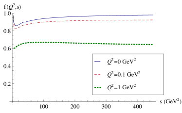
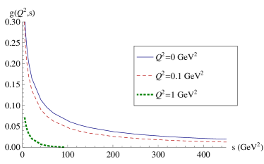
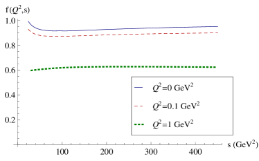
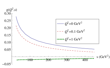
Figure 2: (Color online) Mandelstam-$s$ dependence of the physical and spurious $D^{+}$ (first row) and $B^{-}$ (second row) electromagnetic form factors $f(Q^{2},s)$ and $g(Q^{2},s)$, respectively, for different values of $Q^{2}$ ($0$ GeV² solid, $0.1$ GeV² dashed, $1$ GeV² dotted) calculated with the oscillator wave function, Eq. (35), and (mass) parameters given in the sequel.

The Mandelstam-$s$ dependence of these form factors for a few values of the momentum transfer $Q^{2}$ is plotted in Fig. 2 for $D^{+}$ and $B^{-}$ mesons, respectively. What we observe is that the spurious form factor $g(Q^{2},s)$ goes to zero for $s\rightarrow\infty$ and that the $s$-dependence of the physical form factor $f(Q^{2},s)$ vanishes with increasing $s$. It is therefore suggestive to take the $s\rightarrow\infty$ limit to get rid of cluster-separability violating effects and obtain sensible results for the physical form factors. Taking the $s\rightarrow\infty$ limit means that one extracts the form factor in the infinite momentum frame of the meson. Not surprisingly, for light-light systems the resulting analytical expression for the electromagnetic form factor of a pseudoscalar meson is then seen to be equivalent with the usual front-form result, obtained from a one-body current in the $q^{+}=0$ frame Biernat et al. (2009). For heavy-light systems the situation becomes more intricate. Looking more closely at the form factors for $D^{+}$ and $B^{-}$ (cf. Fig. 2) we observe that the rate of convergence to the $s\rightarrow\infty$ limit decreases with increasing heavy-quark mass. In order to extract sensible results for the Isgur-Wise function one thus has to be very careful when taking the heavy-quark limit $m_{Q}\rightarrow\infty$.

III.2 Decay form factors

III.2.1 P $\rightarrow$ P transition

As in the electromagnetic case a weak pseudoscalar-to-pseudoscalar transition current with the correct transformation properties under Lorentz transformations is obtained from Eq. (30) by applying the canonical boost $B_{c}(\underline{v})$ that connects physical momenta with CM momenta:

$$J^{\nu}_{B\rightarrow D}(\vec{\underline{p}}_{D}^{\prime};\vec{\underline{p}}_{B}):=[B_{c}(\underline{v})]^{\nu}_{\phantom{\nu}\rho}J_{B\rightarrow D}^{\rho}(\vec{\underline{k}}_{D}^{\prime};\vec{\underline{k}}_{B})\,.$$ (37)

An appropriate covariant decomposition of this 4-vector current which holds for arbitrary values of $\vec{\underline{p}}_{B}$ and $\vec{\underline{p}}_{D}^{\prime}$ takes on the form Wirbel et al. (1985)

$$J^{\nu}_{B\rightarrow D}(\vec{\underline{p}}_{D}^{\prime};\vec{\underline{p}}_{B})$$ (38)

$$=\left((\underline{p}_{B}+\underline{p}_{D}^{\prime})^{\nu}-\frac{m^{2}_{B}-m^{2}_{D}}{\underline{q}^{2}}\,\underline{q}^{\nu}\right)F_{1}(\underline{q}^{2})$$

$$\phantom{=}+\frac{m_{B}^{2}-m_{D}^{2}}{\underline{q}^{2}}\,\underline{q}^{\nu}F_{0}(\underline{q}^{2})\,,$$

with the time-like 4-momentum transfer $\underline{q}=(\underline{p}_{B}-\underline{p}_{D})$. Unlike the electromagnetic case wrong cluster properties of the Bakamjian-Thomas construction do not entail unphysical properties of the weak decay current $J^{\nu}_{B\rightarrow D}(\vec{\underline{p}}_{D}^{\prime};\vec{\underline{p}}_{B})$ if the microscopic expression, Eq. (30), is inserted on the right-hand-side of Eq. (37). One neither needs additional unphysical covariants to span the 4-vector $J^{\nu}_{B\rightarrow D}$, nor do the form factors exhibit a dependence on Lorentz invariants different $\underline{q}^{2}$.

The finding that wrong cluster properties of the Bakamjian-Thomas construction do not have obvious physical consequences for the weak decay current $J^{\nu}_{B\rightarrow D}$, whereas they lead to unphysical features of the electromagnetic current $\tilde{J}_{[\alpha]}^{\nu}$, has essentially three reasons:

• Only the final state of the decay process is affected by wrong cluster properties, since the initial state is just the confined quark-antiquark pair with no additional particle present. In electron scattering off a bound system the presence of the electron modifies the bound-state wave function in both, the initial and the final states.

• There is no constraint from current conservation for the decay current $J^{\nu}_{B\rightarrow D}$ such that both 4-vectors, $(\underline{p}_{B}+\underline{p}_{D}^{\prime})$ and $\underline{q}=(\underline{p}_{B}-\underline{p}_{D}^{\prime})$, can be used to express the decay current (cf. Eq. (38)). As it turns out, this suffices. The electromagnetic current $\tilde{J}_{[\alpha]}^{\nu}$, on the other hand, is conserved. It thus cannot have a component into the direction of the momentum transfer $(\underline{p}_{\alpha}-\underline{p}_{\alpha}^{\prime})$, but is also not just proportional to $(\underline{p}_{\alpha}+\underline{p}_{\alpha}^{\prime})$ alone. Therefore one is forced to introduce the unphysical covariant $(\underline{p}_{e}+\underline{p}_{e}^{\prime})$.

• Both, the electromagnetic and the weak form factors are functions of $|\vec{\underline{q}}|$, the modulus of the 3-momentum transfer between the meson in the incoming and outgoing state. Since form factors are frame independent quantities it should be possible to express $|\vec{q}|$ in terms of Lorentz-invariant quantities. In the case of the weak decay $|\vec{\underline{q}}|^{2}$ and $\underline{q}_{\mu}\underline{q}^{\mu}$ are directly related (see below). In the case of electron scattering one needs in general Mandelstam $s$ and $t=\underline{q}_{\mu}\underline{q}^{\mu}$ to express $|\vec{q}|^{2}$. This is the reason why the weak form factors can be written as functions of $\underline{q}_{\mu}\underline{q}^{\mu}$ only, whereas the electromagnetic form factors exhibit an additional (unphysical) dependence on Mandelstam $s$.

The observation that $J^{\nu}_{B\rightarrow D}$ does not exhibit unphysical features does not necessarily mean that there are no problems with wrong cluster properties within our approach in the decay process. As mentioned above wrong cluster properties could still affect the wave function of the final state. But, unlike the electromagnetic case, there is no simple way to separate corresponding contributions in the decay current. The emergence of heavy-quark symmetry, which relates electromagnetic and weak decay form factors, however, will let us conclude that such wrong cluster properties become negligible in the heavy-quark limit.

Equation (38) is a general representation for the weak decay current which holds in any inertial frame. A convenient choice for the extraction of the decay form factors $F_{0}(\underline{q}^{2})$ and $F_{1}(\underline{q}^{2})$ is the CM frame ($\vec{v}=\vec{0}$) in which

$$\underline{k}_{B}=\left(\begin{array}[]{c}m_{B}\\ 0\\ 0\\ 0\end{array}\right)\quad\hbox{and}\quad\underline{k}_{D}^{\prime}=\left(\begin{array}[]{c}\sqrt{m_{D}^{2}+\kappa_{D}^{2}}\\ \kappa_{D}\\ 0\\ 0\end{array}\right)$$ (39)

with

$$\kappa_{D}^{2}=\frac{1}{4m_{B}^{2}}(m_{B}^{2}+m_{D}^{2}-\underline{q}^{2})^{2}-m_{D}^{2}\,.$$ (40)

The modulus of the $D$ meson CM momentum $\kappa_{D}=|\underline{\vec{k}}_{D}^{\prime}|$ is thus restricted by $0\leq\kappa_{D}^{2}\leq(m_{B}^{2}-m_{D}^{2})^{2}/(4m_{B}^{2})$. As in the electromagnetic case the momentum is transferred in $x$-direction. The allowed values of the 4-momentum transfer squared are

$$0\leq\underline{q}^{2}\leq(m_{B}-m_{D})^{2}\,.$$ (41)

The $\nu=2,3$ components of the weak transition current $J^{\nu}_{B\rightarrow D}$ vanish in this kinematics. As it should be, the non-zero $\nu=0,1$ components of $J^{\nu}_{B\rightarrow D}$ are solely determined by the vector part ($\propto\gamma^{\nu}$) of the $Wbc$-vertex. The axial-vector part ($\propto\gamma^{\nu}\gamma^{5}$) of the vertex does not contribute to the $B\rightarrow D$ transition. The form factors $F_{0}(\underline{q}^{2})$ and $F_{1}(\underline{q}^{2})$ can be determined uniquely by projecting onto the corresponding 4-vectors:

$$F_{0}(\underline{q}^{2})=\frac{1}{m_{B}^{2}-m_{D}^{2}}\,\underline{q}_{\nu}J_{B\rightarrow D}^{\nu}(\vec{\underline{k}}_{D}^{\prime};\vec{\underline{k}}_{B})\,,$$ (42)

$$F_{1}(\underline{q}^{2})=-\frac{\underline{q}^{2}}{4m_{B}^{2}m_{D}^{2}}\left[\left(\frac{m_{B}^{2}+m_{D}^{2}-\underline{q}^{2}}{2m_{B}m_{D}}\right)^{2}-1\right]^{-1}$$

$$\times\left((\underline{p}_{B}+\underline{p}_{D}^{\prime})_{\nu}-\frac{m^{2}_{B}-m^{2}_{D}}{\underline{q}^{2}}\,\underline{q}_{\nu}\right)J_{B\rightarrow D}^{\nu}(\vec{\underline{k}}_{D}^{\prime};\vec{\underline{k}}_{B})\,.$$

The constraint $F_{0}(0)=F_{1}(0)$, that eliminates the spurious pole at $\underline{q}^{2}=0$, is automatically satisfied for the form factors calculated from our transition current, Eq. (30).

III.2.2 P $\rightarrow$ V transition

The weak pseudoscalar-to-vector transition current with the correct transformation properties under Lorentz transformations is obtained from Eq. (31) by applying again the canonical boost $B_{c}(\underline{v})$ that connects physical momenta with CM momenta. Linked with this boost is a Wigner rotation of the vector-meson spin:

$$J^{\nu}_{B\rightarrow D^{\ast}}(\vec{\underline{p}}_{D^{\ast}}^{\prime},\underline{\sigma}^{\prime}_{D^{\ast}};\vec{\underline{p}}_{B}):=[B_{c}(\underline{v})]^{\nu}_{\phantom{\nu}\rho}J_{B\rightarrow D^{\ast}}^{\rho}(\vec{\underline{k}}_{D^{\ast}}^{\prime},\underline{\mu}^{\prime}_{D^{\ast}};\vec{\underline{k}}_{B})$$

$$\hskip 71.13188pt\times D^{1\ast}_{\underline{\mu}^{\prime}_{D^{\ast}}\underline{\sigma}^{\prime}_{D^{\ast}}}\left[R^{-1}_{\mathrm{W}}\!\left({\underline{k}}_{D^{\ast}}^{\prime}/m_{D^{\ast}},B_{c}(v)\right)\right]\,.$$

A common covariant decomposition of this 4-vector current has the form Wirbel et al. (1985)

$$J^{\nu}_{B\rightarrow D^{\ast}}(\vec{\underline{p}}_{D^{\ast}}^{\prime},\underline{\sigma}^{\prime}_{D^{\ast}};\vec{\underline{p}}_{B})$$ (45)

$$= \frac{2i\epsilon^{\nu\mu\rho\sigma}}{m_{B}+m_{D^{*}}}\,\epsilon^{*}_{\mu}(\vec{\underline{p}}_{D^{\ast}}^{\prime},\underline{\sigma}^{\prime}_{D^{\ast}})\,\underline{p}^{\prime}_{D^{\ast}\rho}\,\underline{p}_{B\sigma}\,V(\underline{q}^{2})$$

$$-(m_{B}+m_{D^{*}})\,\epsilon^{*\nu}(\vec{\underline{p}}_{D^{\ast}}^{\prime},\underline{\sigma}^{\prime}_{D^{\ast}})\,A_{1}(\underline{q}^{2})$$

$$+\frac{\epsilon^{*}(\vec{\underline{p}}_{D^{\ast}}^{\prime},\underline{\sigma}^{\prime}_{D^{\ast}})\cdot\underline{q}}{m_{B}+m_{D^{*}}}\,(\underline{p}_{B}+\underline{p}_{D^{\ast}}^{\prime})^{\nu}\,A_{2}(\underline{q}^{2})$$

$$+2m_{D^{*}}\,\frac{\epsilon^{*}(\vec{\underline{p}}_{D^{\ast}}^{\prime},\underline{\sigma}^{\prime}_{D^{\ast}})\cdot\underline{q}}{\underline{q}^{2}}\,\underline{q}^{\nu}\,A_{3}(\underline{q}^{2})$$

$$-2m_{D^{*}}\,\frac{\epsilon^{*}(\vec{\underline{p}}_{D^{\ast}}^{\prime},\underline{\sigma}^{\prime}_{D^{\ast}})\cdot\underline{q}}{\underline{q}^{2}}\,\underline{q}^{\nu}\,A_{0}(\underline{q}^{2})\,,$$

with $\epsilon^{*}(\vec{\underline{p}}_{D^{\ast}}^{\prime},\underline{\sigma}^{\prime}_{D^{\ast}})$ being the polarization 4-vector of the $D^{\ast}$ meson and $A_{3}(\underline{q}^{2})$ the linear combination

$$A_{3}(\underline{q}^{2})=\frac{m_{B}+m_{D^{\ast}}}{2m_{D^{\ast}}}\,A_{1}(\underline{q}^{2})-\frac{m_{B}-m_{D^{\ast}}}{2m_{D^{\ast}}}A_{2}(\underline{q}^{2})\,.$$ (46)

The constraint $A_{3}(0)=A_{0}(0)$, that holds automatically for the form factors calculated from our transition current, Eq. (31), guarantees that there is no pole at $\underline{q}^{2}=0$. As for the $B\rightarrow D$ transition wrong cluster properties of the Bakamjian-Thomas construction do not lead to unphysical features of the $J^{\nu}_{B\rightarrow D^{\ast}}$ decay current. The vector $V(\underline{q}^{2})$ and the axial-vector form factors $A_{i}(\underline{q}^{2})$ are determined by the vector part ($\propto\gamma^{\nu}$) and the axial-vector part ($\propto\gamma^{\nu}\gamma^{5}$) of the $Wbc$-vertex, respectively.

Taking the same kinematics as for the $B\rightarrow D$ decay (cf. Eq. (39)) the polarization vectors $\epsilon(\underline{\vec{k}}^{\prime}_{D^{\ast}},\underline{\mu}_{D^{\ast}}^{\prime})$ are given by:

$$\epsilon(\underline{\vec{k}}^{\prime}_{D^{\ast}},\pm 1) = \frac{1}{\sqrt{2}}(\mp\frac{\kappa_{D^{\ast}}}{m_{D^{\ast}}},\mp\sqrt{1+(\frac{\kappa_{D^{\ast}}}{m_{D^{\ast}}})^{2}},-i,0)\,,$$

$$\epsilon(\underline{\vec{k}}^{\prime}_{D^{\ast}},0) = (0,0,0,1)\,.$$ (47)

This kinematics leads to 10 non-vanishing current matrix elements $J^{2}(0)$, $J^{3}(0)$, $J^{\mu}(\pm 1)$, $\mu=0,1,2,3$. Here we have introduced the short-hand notation $J^{\nu}(\underline{\mu}^{\prime}_{D^{\ast}}):=J^{\nu}_{B\rightarrow D^{\ast}}(\vec{\underline{k}}_{D^{\ast}}^{\prime},\underline{\mu}^{\prime}_{D^{\ast}};\vec{\underline{k}}_{B})$. $J^{\mu}(1)$ and $J^{\mu}(-1)$ are related by space reflection. We are thus left with 6 current matrix elements with only 4 of them being independent. The form factors $A_{0}$ and $A_{2}$ enter only $J^{0}(1)$ and $J^{1}(1)$. $J^{2}(0)$, $J^{3}(0)$, $J^{0}(1)$ and $J^{1}(1)$ constitute thus an appropriate set of current matrix elements from which all the $P\rightarrow V$ decay form factors can be extracted. Instead of solving the linear equations which relate the form factors to the current matrix elements $J^{\nu}(\underline{\mu}^{\prime}_{D^{\ast}})$ we express the form factors again in terms of appropriate projections:

$$V(\underline{q}^{2}) = \frac{i(m_{B}+m_{D^{\ast}})}{2m_{B}^{2}m_{D^{\ast}}^{2}}\left[\left(\frac{m_{B}^{2}+m_{D^{\ast}}^{2}-\underline{q}^{2}}{2m_{B}m_{D^{\ast}}}\right)^{2}-1\right]^{-1}$$ (48)

$$\times\epsilon_{\mu}(\vec{\underline{k}}_{D^{\ast}}^{\prime},\underline{\mu}^{\prime}_{D^{\ast}}=0)\,\underline{k}^{\prime}_{D^{\ast}\rho}\,\underline{k}_{B\sigma}\,$$

$$\times\epsilon_{\nu}^{\phantom{\nu}\mu\rho\sigma}J^{\nu}_{B\rightarrow D^{\ast}}(\vec{\underline{k}}_{D^{\ast}}^{\prime},\underline{\mu}^{\prime}_{D^{\ast}}=0;\vec{\underline{k}}_{B})\,,$$

$$A_{0}(\underline{q}^{2}) = \frac{1}{\sqrt{2}m_{B}m_{D^{\ast}}}\left[\left(\frac{m_{B}^{2}+m_{D^{\ast}}^{2}-\underline{q}^{2}}{2m_{B}m_{D^{\ast}}}\right)^{2}-1\right]^{-1/2}$$ (49)

$$\times\underline{q}_{\nu}J^{\nu}_{B\rightarrow D^{\ast}}(\vec{\underline{k}}_{D^{\ast}}^{\prime},\underline{\mu}^{\prime}_{D^{\ast}}=1;\vec{\underline{k}}_{B})\,,$$

$$A_{1}(\underline{q}^{2}) = \frac{1}{m_{B}+m_{D^{\ast}}}\,\epsilon_{\nu}(\vec{\underline{k}}_{D^{\ast}}^{\prime},\underline{\mu}^{\prime}_{D^{\ast}}=0)\,$$ (50)

$$\times J^{\nu}_{B\rightarrow D^{\ast}}(\vec{\underline{k}}_{D^{\ast}}^{\prime},\underline{\mu}^{\prime}_{D^{\ast}}=0;\vec{\underline{k}}_{B})\,.$$

The expression for $A_{2}(\underline{q}^{2})$ is a little bit more complicated:

$$A_{2}(\underline{q}^{2})\! = \!\!\frac{\underline{q}^{2}(m_{B}+m_{D^{\ast}})}{4m_{B}^{2}m_{D^{\ast}}^{2}}\left[\left(\frac{m_{B}^{2}+m_{D^{\ast}}^{2}-\underline{q}^{2}}{2m_{B}m_{D^{\ast}}}\right)^{2}\!\!\!\!-1\right]^{-1}$$

$$\times\Bigg{\{}\frac{\sqrt{2}}{m_{B}}\left[\left(\frac{m_{B}^{2}+m_{D^{\ast}}^{2}-\underline{q}^{2}}{2m_{B}m_{D^{\ast}}}\right)^{2}\!\!\!\!-1\right]^{-1/2}$$

$$\phantom{\times\Bigg{\{}}\times\left((\underline{p}_{B}+\underline{p}_{D^{\ast}}^{\prime})-\frac{m^{2}_{B}-m^{2}_{D^{\ast}}}{\underline{q}^{2}}\,\underline{q}\right)_{\nu}$$

$$\phantom{\times\Bigg{\{}}\times J_{B\rightarrow D^{\ast}}^{\nu}(\vec{\underline{k}}_{D^{\ast}}^{\prime},\underline{\mu}^{\prime}_{D^{\ast}}=1;\vec{\underline{k}}_{B})$$

$$\phantom{\times}-\left[1-\frac{m_{B}^{2}-m_{D^{\ast}}^{2}}{\underline{q}^{2}}\right]\epsilon_{\nu}(\vec{\underline{k}}_{D^{\ast}}^{\prime},\underline{\mu}^{\prime}_{D^{\ast}}=0)$$

$$\phantom{\times\Bigg{\{}}\times J^{\nu}_{B\rightarrow D^{\ast}}(\vec{\underline{k}}_{D^{\ast}}^{\prime},\underline{\mu}^{\prime}_{D^{\ast}}=0;\vec{\underline{k}}_{B})\Bigg{\}}\,.$$

Having derived analytical expressions for the electromagnetic and weak currents and form factors we are now going to study their properties in the heavy-quark limit.

IV The heavy-quark limit

In the heavy-quark limit the masses of the heavy quarks and, consequently, the masses of the heavy hadrons are sent to infinity. This leads to additional symmetries which will be discussed later. With the hadron masses also their momenta go to infinity. What, however, stays finite is the product $\underline{v}_{\alpha}\cdot\underline{v}_{\alpha^{(\prime)}}^{\prime}$ of the hadron 4-velocities. One is then interested in the dependence of form factors on the (finite) velocity product $\underline{v}_{\alpha}\cdot\underline{v}_{\alpha^{(\prime)}}^{\prime}$. Thus it makes more sense to characterize the state of a heavy hadron by its velocity rather than by its momentum. To be more precise, the limit $m_{Q}\rightarrow\infty$ has to be taken in such a way that

$$\underline{v}_{\alpha}\cdot\underline{v}_{\alpha^{(\prime)}}^{\prime}=\frac{\underline{k}_{\alpha}\cdot\underline{k}_{\alpha^{(\prime)}}^{\prime}}{m_{\alpha}m_{\alpha^{(\prime)}}}$$ (52)

stays constant. In this limit both, the binding energy and the light-quark mass, become negligible, i.e.

$$m_{Q^{(\prime)}}=m_{\alpha^{(\prime)}}\quad\hbox{and}\quad\frac{m_{q}}{m_{Q^{(\prime)}}}=0\quad\hbox{for}\quad m_{Q^{(\prime)}}\rightarrow\infty\,.$$ (53)

Furthermore it is assumed that the meson wave functions do not depend on the flavor of the heavy quarks when the masses of the heavy quarks go to infinity. This is our precise definition of the “heavy-quark limit”  (h.q.l.).

IV.1 Space-like momentum transfer

Let us start with the heavy-quark limit of the electromagnetic pseudoscalar-meson current $\tilde{J}_{[\alpha]}^{\nu}(\vec{\underline{k}}_{\alpha}^{\,\prime};\vec{\underline{k}}_{\alpha})$ (cf. Eqs. (19) and (20)). The first step towards the heavy-quark limit is to express the meson momenta and the momenta of the heavy quarks in terms of velocities. To this aim we note that

$$Q=\sqrt{-(\underline{k}_{\alpha}-\underline{k}_{\alpha}^{\prime})^{2}}=2m_{\alpha}\sqrt{\frac{\underline{v}_{\alpha}\cdot\underline{v}_{\alpha}^{\prime}-1}{2}}=:2m_{\alpha}u\,.$$ (54)

This means, in particular, that not only the heavy-quark mass, but also the momentum transfer goes to infinity, when taking the heavy-quark limit. As a consequence $\tilde{J}_{\bar{q}}^{\nu}(\vec{\underline{k}}_{\alpha}^{\,\prime};\vec{\underline{k}}_{\alpha})$, the part of the current in which the momentum is transferred to the light antiquark, vanishes. The formal reason is that the wave-function overlap vanishes (exponentially) when the light antiquark has to absorb an infinite amount of momentum. It thus remains to investigate the heavy-quark limit of $\tilde{J}_{Q}^{\nu}(\vec{\underline{k}}_{\alpha}^{\,\prime};\vec{\underline{k}}_{\alpha})$, i.e. the part of the current in which the momentum is transferred to the heavy quark. Taking the parametrization of meson momenta that has been defined in Eq. (36) and going over to velocities we have:

$$\underline{k}_{\alpha}=m_{\alpha}{\begin{pmatrix}\sqrt{1+\nu_{\alpha}^{2}}\\ -u\\ 0\\ \sqrt{\nu_{\alpha}^{2}-u^{2}}\end{pmatrix}}=m_{\alpha}{\underline{v}_{\alpha}}\,,$$

(55)

$$\underline{k}_{\alpha}^{\prime}=m_{\alpha}{\begin{pmatrix}\sqrt{1+\nu_{\alpha}^{2}}\\ u\\ 0\\ \sqrt{\nu_{\alpha}^{2}-u^{2}}\end{pmatrix}}=m_{\alpha}{\underline{v}_{\alpha}^{\prime}}\,,$$

where $\nu_{\alpha}=|\underline{\vec{v}}_{\alpha}|=|\underline{\vec{v}}_{\alpha}^{\prime}|$ and $u$ is the shorthand notation introduced in Eq. (54). The modulus of the 4-momentum transfer squared $Q^{2}=-q_{\mu}q^{\mu}$ and our new variable $\underline{v}_{\alpha}\cdot\underline{v}_{\alpha}^{\prime}$ are then related by

$$Q^{2}=2m_{\alpha}^{2}(\underline{v}_{\alpha}\cdot\underline{v}_{\alpha}^{\prime}-1)$$ (56)

which means that

$$\underline{v}_{\alpha}\cdot\underline{v}_{\alpha}^{\prime}\geq 1$$

for elastic electron-meson scattering. Using now that

$$\underline{\vec{k}}_{\alpha}^{\,(\prime)}\,,\vec{k}_{Q}^{\,(\prime)}\,\stackrel{{\scriptstyle\mathrm{h.q.l.}}}{{\longrightarrow}}\,m_{\alpha}\,\underline{\vec{v}}_{\alpha}^{\,(\prime)}\,,\quad\frac{|\vec{k}_{\bar{q}}^{\,(\prime)}|}{m_{Q}}\,,\frac{|\vec{\tilde{k}}_{\bar{q}}^{\,(\prime)}|}{m_{Q}}\,,\frac{|\vec{\tilde{k}}_{Q}^{\,(\prime)}|}{m_{Q}}\stackrel{{\scriptstyle\mathrm{h.q.l.}}}{{\longrightarrow}}0\,,\quad\hbox{and}\quad{\vec{v}}_{Q\bar{q}}^{\,(\prime)}\stackrel{{\scriptstyle\mathrm{h.q.l.}}}{{\longrightarrow}}\underline{\vec{v}}_{\alpha}^{\,(\prime)}\,,$$ (57)

the Wigner rotations of the heavy-quark spin become the identity in the heavy-quark limit and the kinematical factors in the pseudoscalar meson current $\tilde{J}_{Q}^{\nu}(\vec{\underline{k}}_{\alpha}^{\,\prime};\vec{\underline{k}}_{\alpha})$ (cf. Eq. (20)) simplify considerably:

$$J^{\nu}_{Q}(\vec{\underline{k}}_{\alpha}^{\prime},\vec{\underline{k}}_{\alpha})\quad\stackrel{{\scriptstyle\mathrm{h.q.l.}}}{{\longrightarrow}}\quad m_{\alpha}\tilde{J}^{\nu}_{\infty}(\vec{\underline{v}}_{\alpha}^{\prime},\vec{\underline{v}}_{\alpha}) = m_{\alpha}\int\,\frac{d^{3}\tilde{k}_{\bar{q}}^{\prime}}{4\pi}\,\sqrt{\frac{\omega_{\tilde{k}_{\bar{q}}}}{\omega_{\tilde{k}^{\prime}_{\bar{q}}}}}\,\bigg{\{}\!\sum_{\mu_{Q},\mu_{Q}^{\prime}=\pm\frac{1}{2}}\!\!\!\bar{q}_{\mu_{Q}^{\prime}}(\vec{\underline{v}}_{\alpha}^{\,\prime})\,\gamma^{\nu}\,u_{\mu_{Q}}(\vec{\underline{v}}_{\alpha})$$

$$\times\frac{1}{2}\,D^{1/2}_{\mu_{Q}\mu_{Q}^{\prime}}\!\left[\!R^{-1}_{\mathrm{W}}\!\left(\frac{\tilde{k}_{\bar{q}}}{m_{\bar{q}}},B_{c}(\underline{v}_{\alpha})\right)\,\!R_{\mathrm{W}}\!\left(\frac{\tilde{k}_{\bar{q}}^{\prime}}{m_{\bar{q}}},B_{c}(\underline{v}_{\alpha}^{\prime})\right)\,\right]\bigg{\}}\,\psi^{\ast}\,(|\vec{\tilde{k}}_{\bar{q}}^{\prime}|)\,\psi\,(|\vec{\tilde{k}}_{\bar{q}}|)\,\,.$$

One can see immediately that the integrand is independent of the heavy quark mass. The only dependencies showing up are those on the integration variables $\vec{\tilde{k}}_{\bar{q}}^{\,\prime}$  and on the meson velocities $\vec{\underline{v}}_{\alpha}^{\,(\prime)}$. The term within the curly brackets comes from the spin of the quarks. For spinless quarks it would coincide with the pointlike current of the pseudoscalar meson $(\underline{v}_{\alpha}+\underline{v}_{\alpha}^{\prime})^{\nu}$. Dropping this factor the integral on the right-hand side of Eq. (IV.1) would already give the Isgur-Wise function for a scalar meson composed of spinless quarks. The general covariant structure of $\tilde{J}^{\nu}_{\infty}(\vec{\underline{v}}_{\alpha}^{\prime},\vec{\underline{v}}_{\alpha})$ for spin-1/2 quarks follows from Eq. (34) by expressing the momenta in terms of velocities

$$\tilde{J}^{\nu}_{\infty}(\vec{\underline{v}}_{\alpha}^{\prime},\vec{\underline{v}}_{\alpha}) = (\underline{v}_{\alpha}+\underline{v}_{\alpha}^{\,\prime})^{\nu}\,\tilde{f}(\underline{v}_{\alpha}\cdot\underline{v}_{\alpha}^{\prime},\nu_{\alpha})$$ (59)

$$+\frac{m_{e}}{m_{\alpha}}(\underline{v}_{e}+\underline{v}_{e}^{\,\prime})^{\nu}\,\tilde{g}(\underline{v}_{\alpha}\cdot\underline{v}_{\alpha}^{\prime},\nu_{\alpha})\,,$$

where

$$\frac{m_{e}}{m_{\alpha}}(\underline{v}_{e}+\underline{v}_{e}^{\,\prime})=2(\nu_{\alpha},0,0,\sqrt{\nu_{\alpha}^{2}-u^{2}})\,.$$ (60)

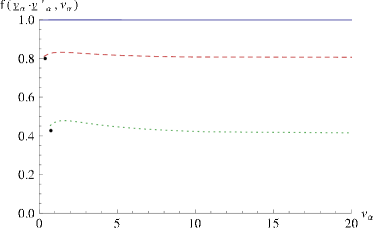
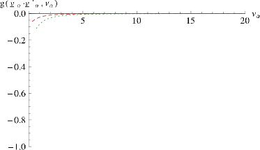
Figure 3: (Color online) Physical and spurious electromagnetic form factors, $\tilde{f}(\underline{v}_{\alpha}\cdot\underline{v}_{\alpha}^{\prime},\nu_{\alpha})$ and $\tilde{g}(\underline{v}_{\alpha}\cdot\underline{v}_{\alpha}^{\prime},\nu_{\alpha})$, of a heavy-light pseudoscalar meson in the heavy-quark limit with the model parameters being the same as in Fig. 2. Their dependence on the modulus of the meson velocities $\nu_{\alpha}$ is plotted for different values of $\underline{v}_{\alpha}\cdot\underline{v}_{\alpha}^{\prime}$ ($1$ solid, $1.2$ dashed, $2$ dotted). The black dots in the left figure are the values for the Isgur-Wise function directly calculated in the Breit frame ($\nu_{\alpha}=u$), where $\tilde{f}(\underline{v}_{\alpha}\cdot\underline{v}_{\alpha}^{\prime},\nu_{\alpha})$ and $\tilde{g}(\underline{v}_{\alpha}\cdot\underline{v}_{\alpha}^{\prime},\nu_{\alpha})$ cannot be separated.

As it turns out and as it is indicated in Eq. (59) $\tilde{J}^{\nu}_{\infty}(\vec{\underline{v}}_{\alpha}^{\prime},\vec{\underline{v}}_{\alpha})$ still does not have all the desired properties. Effects of wrong cluster properties, that are inherent in our approach, do not go away by taking the heavy-quark limit. It is, in general, not possible to write $\tilde{J}^{\nu}_{\infty}(\vec{\underline{v}}_{\alpha}^{\prime},\vec{\underline{v}}_{\alpha})$ as a product of the covariant $(\underline{v}_{\alpha}+\underline{v}_{\alpha}^{\,\prime})^{\nu}$ times the Isgur-Wise function $\xi(\underline{v}_{\alpha}\cdot\underline{v}_{\alpha}^{\prime})$. One rather needs a second covariant built from the electron velocities. In addition, the form factors are not only functions of $\underline{v}_{\alpha}\cdot\underline{v}_{\alpha}^{\prime}$, but exhibit also a dependence on the modulus of the meson velocities $\nu_{\alpha}$. The latter dependence corresponds to the Mandelstam-$s$ dependence ($\nu_{\alpha}=(\frac{\sqrt{s}}{m_{\alpha}}-\frac{m_{\alpha}}{\sqrt{s}})/2$ with $s=m_{\alpha}^{2}(\underline{v}_{\alpha}+\frac{m_{e}}{m_{\alpha}}\underline{v}_{e})^{2}$) which we have already discussed in Sec. III (cf. Fig. 2) for the case of finite heavy-quark mass and which also occurs in light-light systems Biernat et al. (2009); Biernat (2011). The $\nu_{\alpha}$-dependence of $\tilde{f}(\underline{v}_{\alpha}\cdot\underline{v}_{\alpha}^{\prime},\nu_{\alpha})$ and $\tilde{g}(\underline{v}_{\alpha}\cdot\underline{v}_{\alpha}^{\prime},\nu_{\alpha})$ is displayed in Fig. 3 for different values of $\underline{v}_{\alpha}\cdot\underline{v}_{\alpha}^{\prime}$ with the wave function of the heavy-light system being the one introduced in Eq. (35). One observes that both, the $\nu_{\alpha}$-dependence and the spurious form factor $\tilde{g}(\underline{v}_{\alpha}\cdot\underline{v}_{\alpha}^{\prime},\nu_{\alpha})$ vanish rather quickly with increasing $\nu_{\alpha}$. It is therefore suggestive to identify the Isgur-Wise function $\xi(\underline{v}_{\alpha}\cdot\underline{v}_{\alpha}^{\prime})$ with the $\nu_{\alpha}\rightarrow\infty$ limit of $\tilde{f}(\underline{v}_{\alpha}\cdot\underline{v}_{\alpha}^{\prime},\nu_{\alpha})$. In this limit the unwanted $\nu_{\alpha}$-dependence goes away and $\tilde{J}^{\nu}_{\infty}(\vec{\underline{v}}_{\alpha}^{\prime},\vec{\underline{v}}_{\alpha})$ acquires the expected structure

$$\tilde{J}^{\nu}_{\infty}(\vec{\underline{v}}_{\alpha}^{\prime},\vec{\underline{v}}_{\alpha})\stackrel{{\scriptstyle\nu_{\alpha}\rightarrow\infty}}{{\longrightarrow}}(\underline{v}_{\alpha}+\underline{v}_{\alpha}^{\prime})^{\nu}\,\xi_{\mathrm{IF}}(\underline{v}_{\alpha}\cdot\underline{v}_{\alpha}^{\prime})\,,$$ (61)

with a simple analytical expression for the Isgur-Wise function

$$\xi_{\mathrm{IF}}(\underline{v}_{\alpha}\cdot\underline{v}_{\alpha}^{\prime})=\int\,\frac{d^{3}\tilde{k}_{\bar{q}}^{\prime}}{4\pi}\,\sqrt{\frac{\omega_{\tilde{k}_{\bar{q}}}}{\omega_{\tilde{k}^{\prime}_{\bar{q}}}}}\,\mathcal{S}_{\mathrm{IF}}\,\psi^{\ast}\,(|\vec{\tilde{k}}_{\bar{q}}^{\prime}|)\,\psi\,(|\vec{\tilde{k}}_{\bar{q}}|)\,\,.$$ (62)

Taking the limit $\nu_{\alpha}\rightarrow\infty$ means that the $\gamma^{\ast}M_{\alpha}\rightarrow M_{\alpha}$ subprocess is considered in the infinite-momentum frame of the meson $M_{\alpha}$. This is the reason why a subscript “IF” is attached to the Isgur-Wise function and the spin-rotation factor. The relation between $\omega_{\tilde{k}_{\bar{q}}}$ and $\omega_{\tilde{k}^{\prime}_{\bar{q}}}$ (and hence between $|\vec{\tilde{k}}_{\bar{q}}|$ and $|\vec{\tilde{k}}_{\bar{q}}^{\prime}|$) follows from Eq. (25) and is given by ($2u^{2}=\underline{v}_{\alpha}\cdot\underline{v}_{\alpha}^{\prime}-1$)

$$\omega_{\tilde{k}_{\bar{q}}}=2\tilde{k}^{\prime 1}_{\bar{q}}\,u+2\tilde{k}^{\prime 3}_{\bar{q}}\,u^{2}+\omega_{\tilde{k}^{\prime}_{\bar{q}}}(2u^{2}+1)\,.$$ (63)

The spin-rotation factor $\mathcal{S}_{\mathrm{IF}}$ takes on the form

$$\mathcal{S}_{\mathrm{IF}}=\frac{m_{\bar{q}}+\omega_{\tilde{k}^{\prime}_{\bar{q}}}+\tilde{k}^{\prime 1}_{\bar{q}}\,u}{\sqrt{(m_{\bar{q}}+\omega_{\tilde{k}_{\bar{q}}})(m_{\bar{q}}+\omega_{\tilde{k}^{\prime}_{\bar{q}}})}}\,.$$ (64)

In the infinite-momentum frame the meson moves with large velocity in $z$-direction and the momentum is transferred in transverse direction. It is a special $q^{+}=0$ frame, in which the plus component of the 4-momentum transfer vanishes. Such frames are very popular for form-factor studies in front-form Keister and Polyzou (1991); Simula (1996). Another widely used frame to analyze the $\gamma^{\ast}M_{\alpha}\rightarrow M_{\alpha}$ subprocess is the Breit frame in which the energy-transfer between the meson in the initial and the final states vanishes Lev (1995); Klink (1998a). This corresponds to elastic electron-meson backward scattering in the (overall) center-of-momentum frame and is characterized by the minimal meson momentum necessary for reaching a particular momentum transfer $Q$. In this sense it is just the opposite situation to the infinite-momentum frame, in which the meson momentum goes to infinity. In our case the Breit frame is reached by taking the minimum value for $\nu_{\alpha}$, i.e. $\nu_{\alpha}^{2}=u^{2}=(\underline{v}_{\alpha}\cdot\underline{v}_{\alpha}^{\prime}-1)/2$ (cf. Eq. (IV.1)). If this is done,

$$\tilde{J}^{\nu}_{\infty}(\vec{\underline{v}}_{\alpha}^{\prime},\vec{\underline{v}}_{\alpha}) \stackrel{{\scriptstyle\nu_{\alpha}\rightarrow u}}{{\longrightarrow}} (\underline{v}_{\alpha}+\underline{v}_{\alpha}^{\prime})^{\nu}\,\Big{\{}\tilde{f}(\underline{v}_{\alpha}\cdot\underline{v}_{\alpha}^{\prime},\nu_{\alpha}=u)$$ (65)

$$+\sqrt{\frac{\underline{v}_{\alpha}\cdot\underline{v}_{\alpha}^{\prime}-1}{\underline{v}_{\alpha}\cdot\underline{v}_{\alpha}^{\prime}+1}}\,\tilde{g}(\underline{v}_{\alpha}\cdot\underline{v}_{\alpha}^{\prime},\nu_{\alpha}=u)\Big{\}}$$

$$=:(\underline{v}_{\alpha}+\underline{v}_{\alpha}^{\prime})^{\nu}\,\xi_{\mathrm{B}}(\underline{v}_{\alpha}\cdot\underline{v}_{\alpha}^{\prime})$$

and it is not possible any more to separate the physical form factor $\tilde{f}$ from the unphysical form factor $\tilde{g}$. We therefore denote the resulting combination that occurs as coefficient of the covariant $(\underline{v}_{\alpha}+\underline{v}_{\alpha}^{\prime})^{\nu}$ by $\xi_{\mathrm{B}}(\underline{v}_{\alpha}\cdot\underline{v}_{\alpha}^{\prime})$, i.e. the Isgur-Wise function in the Breit frame. The integral for $\xi_{\mathrm{B}}(\underline{v}_{\alpha}\cdot\underline{v}_{\alpha}^{\prime})$ has the same structure as the one for $\xi_{\mathrm{IF}}(\underline{v}_{\alpha}\cdot\underline{v}_{\alpha}^{\prime})$ (cf. Eq. (62)), namely

$$\xi_{\mathrm{B}}(\underline{v}_{\alpha}\cdot\underline{v}_{\alpha}^{\prime})=\int\,\frac{d^{3}\tilde{k}_{\bar{q}}^{\prime}}{4\pi}\,\sqrt{\frac{\omega_{\tilde{k}_{\bar{q}}}}{\omega_{\tilde{k}^{\prime}_{\bar{q}}}}}\,\mathcal{S}_{\mathrm{B}}\,\psi^{\ast}\,(|\vec{\tilde{k}}_{\bar{q}}^{\prime}|)\,\psi\,(|\vec{\tilde{k}}_{\bar{q}}|)\,\,.$$ (66)

Only the boosts that relate $\tilde{k}_{\bar{q}}^{\prime}$ and $\tilde{k}_{\bar{q}}$ are different. In the Breit frame $\omega_{\tilde{k}_{\bar{q}}}$ and $\omega_{\tilde{k}^{\prime}_{\bar{q}}}$ are connected via

$$\omega_{\tilde{k}_{\bar{q}}}=2\tilde{k}^{\prime 1}_{\bar{q}}\,u\sqrt{u^{2}+1}+\omega_{\tilde{k}^{\prime}_{\bar{q}}}(2u^{2}+1)$$ (67)

and the spin-rotation factor $\mathcal{S}_{\mathrm{B}}$ becomes

$$\mathcal{S}_{\mathrm{B}}=\frac{m_{\bar{q}}+\omega_{\tilde{k}^{\prime}_{\bar{q}}}+\tilde{k}^{\prime 1}_{\bar{q}}\,\frac{u}{\sqrt{u^{2}+1}}}{\sqrt{(m_{\bar{q}}+\omega_{\tilde{k}_{\bar{q}}})(m_{\bar{q}}+\omega_{\tilde{k}^{\prime}_{\bar{q}}})}}\,.$$ (68)

The integrands for the Isgur-Wise function in the infinite-momentum frame and the Breit frame are thus obviously different. Surprisingly, the numerical integration gives the same results for $\xi_{\mathrm{IF}}(\underline{v}_{\alpha}\cdot\underline{v}_{\alpha}^{\prime})$ and $\xi_{\mathrm{B}}(\underline{v}_{\alpha}\cdot\underline{v}_{\alpha}^{\prime})$. This can be seen in Fig. 3, where the results for $\xi_{\mathrm{B}}(\underline{v}_{\alpha}\cdot\underline{v}_{\alpha}^{\prime})$ are indicated by the black dots. These dots should be compared with the right end of the corresponding curves. This suggests that the integrands of $\xi_{\mathrm{IF}}(\underline{v}_{\alpha}\cdot\underline{v}_{\alpha}^{\prime})$ and $\xi_{\mathrm{B}}(\underline{v}_{\alpha}\cdot\underline{v}_{\alpha}^{\prime})$ are related by a change of integration variables. And indeed, the expressions for the energies in Eqs. (63) and (67) are connected via a simple rotation:

$$\begin{pmatrix}\tilde{k}_{\bar{q}}^{\prime\,1}\\ \tilde{k}_{\bar{q}}^{\prime\,3}\end{pmatrix}_{\mathrm{IF}}=\frac{1}{\sqrt{u^{2}+1}}\begin{pmatrix}1&-u\\ u&1\end{pmatrix}\begin{pmatrix}\tilde{k}_{\bar{q}}^{\prime\,1}\\ \tilde{k}_{\bar{q}}^{\prime\,3}\end{pmatrix}_{\mathrm{B}}\,.$$ (69)

Applying this change of variables to the spin-rotation factor $\mathcal{S}_{\mathrm{IF}}$ one ends up with $\mathcal{S}_{\mathrm{B}}$ plus an additional term which is an odd function of $\tilde{k}_{\bar{q}\mathrm{B}}^{\prime\,3}$ that vanishes upon integration. Our result for the Isgur-Wise function is thus independent on whether we extract it in the Breit frame or in the infinite-momentum frame. We therefore will drop the subscripts “IF” and “B”. For further purposes we will take the somewhat simpler analytical Breit-frame expression

$$\xi(v\cdot v^{\prime})=\int\,\frac{d^{3}\tilde{k}_{\bar{q}}^{\prime}}{4\pi}\,\sqrt{\frac{\omega_{\tilde{k}_{\bar{q}}}}{\omega_{\tilde{k}^{\prime}_{\bar{q}}}}}\,\mathcal{S}\,\psi^{\ast}\,(|\vec{\tilde{k}}_{\bar{q}}^{\prime}|)\,\psi\,(|\vec{\tilde{k}}_{\bar{q}}|)\,\,.$$ (70)

with

$$\omega_{\tilde{k}_{\bar{q}}}=\tilde{k}^{\prime 1}_{\bar{q}}\,\sqrt{(v\cdot v^{\prime})^{2}-1}+\omega_{\tilde{k}^{\prime}_{\bar{q}}}\,(v\cdot v^{\prime})$$ (71)

and

$$\mathcal{S}=\frac{m_{\bar{q}}+\omega_{\tilde{k}^{\prime}_{\bar{q}}}+\tilde{k}^{\prime 1}_{\bar{q}}\,\sqrt{\frac{{(v\cdot v^{\prime})-1}}{{(v\cdot v^{\prime})+1}}}}{\sqrt{(m_{\bar{q}}+\omega_{\tilde{k}_{\bar{q}}})(m_{\bar{q}}+\omega_{\tilde{k}^{\prime}_{\bar{q}}})}}\,.$$ (72)

as our Isgur-Wise function. Here we have just reexpressed $u$ in terms of $v\cdot v^{\prime}$. As one can check, the Isgur-Wise function introduced in this way is now only a function of $v\cdot v^{\prime}$ and it is correctly normalized, i.e.

$$\xi(v\cdot v^{\prime}=1)=1\,.$$ (73)

Its independence on the heavy-quark mass $m_{Q}$ is one of the consequences of heavy-quark flavor symmetry which is supposed to hold in the heavy-quark limit Isgur and Wise (1989, 1990); Neubert (1994).

Heavy-quark flavor symmetry reaches even further. The heavy flavor in the final state can be replaced by another heavy flavor without affecting the Isgur-Wise function. The physical processes leading to such flavor-changing heavy-to-heavy transitions are, e.g., weak decays. Thus our next aim will be to check whether the heavy-quark limit of the weak $B\rightarrow D$ transition current, as given in Eq. (30), provides the same Isgur-Wise function as the electromagnetic current, Eq. (20).

IV.2 Time-like momentum transfer

Like in the electromagnetic case we rewrite meson and heavy-quark momenta in terms of velocities. The meson momenta that specify our decay kinematics (cf. Eq. (39)) can be directly expressed in terms of $\underline{v}_{B}\cdot\underline{v}^{\prime}_{D^{(\ast)}}$:

$$\underline{k}_{B} = m_{B}\left(\begin{array}[]{c}1\\ 0\\ 0\\ 0\end{array}\right)=m_{B}\underline{v}_{B}\,,$$ (78)

$$\underline{k}_{D^{(\ast)}}^{\prime} = m_{D^{(\ast)}}\left(\begin{array}[]{c}\underline{v}_{B}\cdot\underline{v}^{\prime}_{D^{(\ast)}}\\ \sqrt{(\underline{v}_{B}\cdot\underline{v}^{\prime}_{D^{(\ast)}})^{2}-1}\\ 0\\ 0\end{array}\right)=m_{D^{(\ast)}}\underline{v}_{D^{(\ast)}}\,.$$ (83)

For the decay the momentum transferred between the initial and the final meson is time-like, i.e.

$$0\leq\underline{q}^{2} = (\underline{k}_{B}-\underline{k}_{D^{(\ast)}})^{2}$$

$$=m_{B}^{2}+m_{D^{(\ast)}}^{2}-2m_{B}m_{D^{(\ast)}}\underline{v}_{B}\cdot\underline{v}^{\prime}_{D^{(\ast)}}\leq(m_{B}-m_{D^{(\ast)}})^{2}\,.$$

From Eqs. (78) and (IV.2) we conclude that

$$1\leq\underline{v}_{B}\cdot\underline{v}^{\prime}_{D^{(\ast)}}\leq 1+\frac{(m_{B}-m_{D^{(\ast)}})^{2}}{2m_{B}m_{D^{(\ast)}}}\,.$$ (85)

Note that this $v\cdot v^{\prime}$-interval is also accessible in elastic electron-meson scattering for which only $v\cdot v^{\prime}\geq 1$ must hold. This makes it possible to directly compare the structure of heavy-light mesons as measured in elastic scattering with the structure inferred from the observation of weak decays, although these processes involve space-like and time-like momentum transfers, respectively.

Since the axial-vector contribution of the quark current vanishes for pseudoscalar to pseudoscalar transitions, the heavy-quark limit of the $B\rightarrow D$ transition current, Eq. (30), is given by

$$J^{\nu}_{B\rightarrow D}(\vec{\underline{k}}_{D}^{\prime},\vec{\underline{k}}_{B})\quad\stackrel{{\scriptstyle\mathrm{h.q.l.}}}{{\longrightarrow}}\quad\sqrt{m_{B}m_{D}}\,\tilde{J}^{\nu}_{B\rightarrow D}(\vec{\underline{v}}_{D}^{\prime},\vec{\underline{v}}_{B}) = \sqrt{m_{B}m_{D}}\,\int\,\frac{d^{3}\tilde{k}_{\bar{q}}^{\prime}}{4\pi}\,\sqrt{\frac{\omega_{\tilde{k}_{\bar{q}}}}{\omega_{\tilde{k}^{\prime}_{\bar{q}}}}}\,\bigg{\{}\!\sum_{\mu_{b},\mu_{c}^{\prime}=\pm\frac{1}{2}}\!\!\!\bar{q}_{\mu_{c}^{\prime}}(\vec{\underline{v}}_{D}^{\,\prime})\,\gamma^{\nu}\,u_{\mu_{b}}(\vec{\underline{v}}_{B})$$ (86)

$$\times\frac{1}{2}\,D^{1/2}_{\mu_{b}\mu_{c}^{\prime}}\!\left[\!R_{\mathrm{W}}\!\left(\frac{\tilde{k}^{\prime}_{\bar{q}}}{m_{\bar{q}}},B_{c}(\underline{v}_{D}^{\prime})\right)\,\,\right]\bigg{\}}\,\psi^{\ast}\,(|\vec{\tilde{k}}_{\bar{q}}^{\prime}|)\,\psi\,(|\vec{\tilde{k}}_{\bar{q}}|)\,\,.$$

Here we have made use of Eq. (57) and the fact that the Wigner rotation of the $c$-quark spin becomes the identity. Exploiting the general properties of the Wigner $D$-functions and

$$\bar{q}_{-\mu_{b}}(\vec{\underline{v}}_{D}^{\,\prime})\,\gamma^{\nu}\,u_{\mu_{b}}(\vec{\underline{v}}_{B}) = -\left(\bar{q}_{\mu_{b}}(\vec{\underline{v}}_{D}^{\,\prime})\,\gamma^{\nu}\,u_{-\mu_{b}}(\vec{\underline{v}}_{B})\right)^{\ast}\,,$$

$$\bar{q}_{\mu_{b}}(\vec{\underline{v}}_{D}^{\,\prime})\,\gamma^{\nu}\,u_{\mu_{b}}(\vec{\underline{v}}_{B}) = \sqrt{\frac{2}{\underline{v}_{B}\cdot\underline{v}^{\prime}_{D}+1}}\,(\underline{v}_{B}+\underline{v}^{\prime}_{D})^{\nu}\,,$$

it can be shown that the heavy-quark limit of the $B\rightarrow D$ transition current finally takes on the form

$$\tilde{J}^{\nu}_{B\rightarrow D}(\vec{\underline{v}}_{D}^{\prime},\vec{\underline{v}}_{B})=(\underline{v}_{B}+\underline{v}^{\prime}_{D})^{\nu}\,\xi(\underline{v}_{B}\cdot\underline{v}^{\prime}_{D})\,,$$ (88)

with $\xi(\underline{v}_{B}\cdot\underline{v}^{\prime}_{D})$ being the Isgur-Wise function defined in Eqs. (70)-(72). This proves that heavy-quark flavor symmetry is respected by our appproach to the electroweak structure of heavy-light mesons.

Whereas the Isgur-Wise function is just the heavy-quark limit of the electromagnetic form factor (expressed as function of $v\cdot v^{\prime}$) its relation to the decay form factors $F_{0}$ and $F_{1}$ is a little bit more complicated. By comparing Eq. (88) with Eq. (38) it follows that Neubert and Rieckert (1992)

$$R\,\left[1-\frac{q^{2}}{(m_{B}+m_{D})^{2}}\right]^{-1}\,F_{0}(q^{2})\stackrel{{\scriptstyle\mathrm{h.q.l.}}}{{\longrightarrow}}\,\xi(\underline{v}_{B}\cdot\underline{v}^{\prime}_{D})$$ (89)

and that

$$R\,\,F_{1}(q^{2})\stackrel{{\scriptstyle\mathrm{h.q.l.}}}{{\longrightarrow}}\,\xi(\underline{v}_{B}\cdot\underline{v}^{\prime}_{D})\,,$$ (90)

with

$$R=\frac{2\sqrt{m_{B}m_{D}}}{m_{B}+m_{D}}\,.$$ (91)

For finite heavy quark masses the deviation of the left-hand sides of Eqs. (89) and (90) from the Isgur-Wise function $\xi(\underline{v}_{B}\cdot\underline{v}^{\prime}_{D})$ is a measure for the amount of heavy-quark (flavor) symmetry breaking.

The heavy-quark flavor symmetry is not the only symmetry which is recovered in the heavy-quark limit. There is also a heavy-quark spin symmetry which has its origin in the decoupling of the heavy-quark spin from the spin of the light degrees of freedom. Heavy-quark spin symmetry allows to relate matrix elements involving vector mesons with corresponding ones for pseudoscalar mesons. A particular example is the statement that the current matrix elements of the pseudoscalar-to-vector $B\rightarrow D^{\ast}$ transition are determined by the same Isgur-Wise function as the current matrix elements of the pseudoscalar-to-pseudoscalar $B\rightarrow D$ transition Isgur and Wise (1990, 1989); Neubert (1994).

The heavy-quark limit of the $B\rightarrow D^{\ast}$ transition current, Eq. (31), becomes

$$J^{\nu}_{B\rightarrow D^{\ast}}(\vec{\underline{k}}_{D^{\ast}}^{\prime},\underline{\mu}_{D^{\ast}}^{\prime};\vec{\underline{k}}_{B})$$

$$\downarrow{\mathrm{h.q.l.}}$$

$$\sqrt{m_{B}m_{D}}\,\tilde{J}^{\nu}_{B\rightarrow D^{\ast}}(\vec{\underline{v}}_{D^{\ast}}^{\prime},\underline{\mu}_{D^{\ast}}^{\prime};\vec{\underline{v}}_{B}) =\sqrt{m_{B}m_{D}}\,\int\,\frac{d^{3}\tilde{k}_{\bar{q}}^{\prime}}{4\pi}\,\sqrt{\frac{\omega_{\tilde{k}_{\bar{q}}}}{\omega_{\tilde{k}^{\prime}_{\bar{q}}}}}\,\bigg{\{}\!\sum_{\mu_{b},\mu_{c}^{\prime},\tilde{\mu}_{\bar{q}}^{\prime}=\pm\frac{1}{2}}\!\!\!\!\!\!\bar{q}_{\mu_{c}^{\prime}}(\underline{\vec{v}}_{D^{\ast}}^{\prime})\,\gamma^{\nu}\,(1-\gamma^{5})u_{\mu_{b}}(\underline{\vec{v}}_{B})$$

$$\quad\times\sqrt{2}(-1)^{\frac{1}{2}-\mu_{b}}C^{1\underline{\mu}^{\prime}_{\!D^{\ast}}}_{\frac{1}{2}\mu_{c}^{\prime}\frac{1}{2}\tilde{\mu}_{\bar{q}}^{\prime}}\,D^{1/2}_{\tilde{\mu}_{\bar{q}}^{\prime}-\mu_{b}}\!\left[\!R^{-1}_{\mathrm{W}}\!\left(\frac{\tilde{k}^{\prime}_{\bar{q}}}{m_{\bar{q}}},B^{-1}_{c}(\underline{v}_{D^{\ast}}^{\prime})\right)\right]\bigg{\}}\,\psi^{\ast}_{D^{\ast}}\,(|\vec{\tilde{k}}_{\bar{q}}^{\prime}|)\,\psi_{B}\,(|\vec{\tilde{k}}_{\bar{q}}|)\,.$$

It can now be verified that $\tilde{J}^{\nu}_{B\rightarrow D^{\ast}}(\vec{\underline{v}}_{D^{\ast}}^{\prime},\underline{\mu}_{D^{\ast}}^{\prime};\vec{\underline{v}}_{B})$ has the desired covariant structure Isgur and Wise (1990)

$$\tilde{J}^{\nu}_{B\rightarrow D^{\ast}}(\vec{\underline{v}}_{D^{\ast}}^{\prime},\underline{\mu}_{D^{\ast}}^{\prime};\vec{\underline{v}}_{B}) = i\,\epsilon^{\nu\alpha\beta\gamma}\,\epsilon_{\alpha}(m_{D^{\ast}}\vec{\underline{v}}_{D^{\ast}}^{\prime},\underline{\mu}_{D^{\ast}}^{\prime})\,\underline{v}^{\prime}_{D^{\ast}\beta}\,\underline{v}_{B\gamma}\,\xi(\underline{v}_{B}\cdot\underline{v}^{\prime}_{D^{\ast}})\,,$$ (93)

$$-\left[\epsilon^{\nu}(m_{D^{\ast}}\vec{\underline{v}}_{D^{\ast}}^{\prime},\underline{\mu}_{D^{\ast}}^{\prime})\,(\underline{v}_{B}\cdot\underline{v}^{\prime}_{D^{\ast}}+1)-\underline{v}^{\prime\nu}_{D^{\ast}}\,\epsilon(m_{D^{\ast}}\vec{\underline{v}}_{D^{\ast}}^{\prime},\underline{\mu}_{D^{\ast}}^{\prime})\cdot\underline{v}_{B}\right]\,\xi(\underline{v}_{B}\cdot\underline{v}^{\prime}_{D^{\ast}})\,,$$

with $\xi(\underline{v}_{B}\cdot\underline{v}^{\prime}_{D^{\ast}})$ being again the Isgur-Wise function defined in Eqs. (70)-(72). This proves that also heavy-quark spin symmetry is recovered in the heavy-quark limit within our approach.

By comparing Eq. (93) with Eq. (III.2.2) we finally obtain the relations between the physical $B\rightarrow D^{\ast}$ decay form factors (in the heavy-quark limit) and the Isgur-Wise function Neubert and Rieckert (1992):

$$R^{\ast}\,\left[1-\frac{q^{2}}{(m_{B}+m_{D}^{\ast})^{2}}\right]^{-1}\,A_{1}(q^{2})\stackrel{{\scriptstyle\mathrm{h.q.l.}}}{{\longrightarrow}}\,\xi(\underline{v}_{B}\cdot\underline{v}^{\prime}_{D^{\ast}})\,,$$ (94)

$$R^{\ast}\,\,V(q^{2})\stackrel{{\scriptstyle\mathrm{h.q.l.}}}{{\longrightarrow}}\,\xi(\underline{v}_{B}\cdot\underline{v}^{\prime}_{D^{\ast}})\,,$$ (95)

and

$$R^{\ast}\,\,A_{i}(q^{2})\stackrel{{\scriptstyle\mathrm{h.q.l.}}}{{\longrightarrow}}\,\xi(\underline{v}_{B}\cdot\underline{v}^{\prime}_{D^{\ast}})\,,\quad i=0,2\,,$$ (96)

with

$$R^{\ast}=\frac{2\sqrt{m_{B}m_{D^{\ast}}}}{m_{B}+m_{D^{\ast}}}\,.$$ (97)

If the left-hand sides of Eqs. (94)-(96) are calculated with physical heavy-quark masses, their deviation from the Isgur-Wise function on the right-hand sides and the differences amongst each other can be taken as a measure for the amount of heavy-quark spin symmetry breaking.

V Numerical studies

At this point we want to emphasize that the aim of this paper is not to give quantitative predictions for electroweak heavy-light (transition) form factors based on a sophisticated constituent-quark model. It is rather our intention to demonstrate that the kind of relativistic coupled-channel approach that we are using to identify the electroweak structure of few-body bound states is general enough to provide also sensible results for heavy-light systems. First we note that the electromagnetic and weak currents are solely determined by the bound-state wave function and the constituent-quark masses (cf. Eqs. (20), (30) and (31)). For our numerical studies we adopt the simple harmonic-oscillator wave function already introduced in Eq. (35) and the oscillator and mass parameters quoted there. In order to calculate the weak transition form factors from the currents one also needs the meson masses calculated from the harmonic-oscillator confinement potential (cf. Eqs. (42),(III.2.1) and (48)-(III.2.2)). We take the physical masses, since the theoretically calculated spectrum can always be shifted by adding an appropriate constant to the confinement potential such that the experimentally measured pseudoscalar and vector-meson ground-state masses (which we deal with) are reproduced.

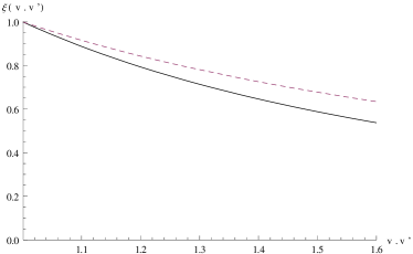
Figure 4: (Color online) Isgur-Wise function (solid line) calculated by means of Eqs. (70)-(72) with the model parameters being the same as in Fig. 2. The dashed line corresponds to spin-rotation factor $\mathcal{S}=1$.

The Isgur-Wise function, as resulting from this simple harmonic-oscillator model, is plotted in Figure 4. The effect of the quark spin onto the Isgur-Wise function can be estimated by comparing the solid with the dashed line. The latter corresponds to the coupling of the photon to spinless quarks and is obtained by setting the spin-rotation factor $\mathcal{S}=1$. The comparison shows the importance of the proper relativistic treatment of the spin rotation when boosting the $Q$-$\bar{q}$ bound-state wave function from the initial to the final state. Here it should be emphasized that it does not matter within our approach whether the Isgur-Wise function is taken as the heavy-quark limit of the electromagnetic $B$-meson form factor or as the heavy-quark limit of any of the $B\rightarrow D^{(\ast)}$ decay form factors, although these processes involve space- and time-like momentum transfers, respectively. In the foregoing section this is proved analytically, but it can also be verified numerically (see the right plots in Figs. 5-7). The authors of Ref. Cheng et al. (1997), from which we have taken our model parameters, have derived two different analytical expressions for the Isgur-Wise function within a front-form approach by taking the heavy-quark limit of the $B\rightarrow D$ and $B\rightarrow D^{\ast}$ decay form factors, respectively. These two expressions are then seen to provide the same numerical results for the Gaussian wave function which we also use, but give different results for the flavor dependent Wirbel-Stech-Bauer wave function Wirbel et al. (1985). From this they conclude that the Wirbel-Stech-Bauer wave function violates heavy-quark symmetry. Our numerical results, obtained with the Gaussian wave function, agree with those of Ref. Cheng et al. (1997) and we are also able to reproduce the value for the slope of the Isgur-Wise function at the normalization point $v\cdot v^{\prime}=1$, namely $\rho^{2}=-\xi^{\prime}(1)=1.24$.

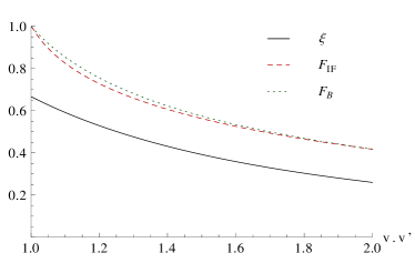
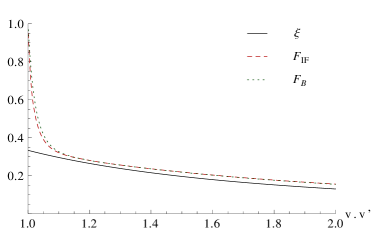
Figure 5: (Color online) Electromagnetic form factors of the $D^{+}$ (left) and $B^{-}$ (right) mesons calculated in the Breit frame (dotted line) and infinite-momentum frame (dashed line) in comparison with the Isgur-Wise function (solid line). For direct comparison the Isgur-Wise function is multiplied by $|Q_{Q}|$, i.e. the charge of the heavy quark. Model parameters are the same as in Fig. 2.

A reasonably simple analytical expression for the Isgur-Wise function in front form can be found in Ref. Cheng et al. (1998). Its structure bears some resemblance to Eqs. (70)-(72), but we have not attempted to prove the equivalence. There are, however, strong hints that such an equivalence holds. In the case of the pion we were able to show analytically that our electromagnetic pion form factor (for space-like momentum transfers) is equivalent with the usual front-form expression that results from the $+$-component of a one-body current in a $q^{+}=0$ frame Biernat et al. (2009). We suppose that this equivalence extends to the case of bound states with unequal-mass constituents and generalizes to electroweak $M\rightarrow M^{\prime}$ transition form factors (for space-like momentum transfers), although we have not tried to prove it analytically. If this is the case, the heavy-quark limit of electroweak heavy-light meson (transition) form factors in front-form and point-form should also lead to the same Isgur-Wise function.

There is still one gap in this reasoning. It refers to form factors in the space-like momentum-transfer region, whereas the authors of Refs. Cheng et al. (1997, 1998) derive their Isgur-Wise function from weak $B\rightarrow D^{(\ast)}$ decay form factors, i.e. in the time-like momentum transfer region. It cannot be taken for granted that the heavy-quark limit of a one-body current, like it is used in Refs.Cheng et al. (1997, 1998), gives the same result for the Isgur-Wise function in the space- and time-like momentum-transfer regions. Going from space- to time-like momentum transfers means that one has to give up the $q^{+}=0$ condition and, as a consequence, $Z$-graphs (i.e. non-valence contributions) may become important Simula (2002). This is confirmed by an analysis of the triangle diagram for $B\rightarrow D^{(\ast)}$ decays within a simple covariant model Bakker et al. (2003). There it is shown that analytic continuation ($q_{\perp}\rightarrow iq_{\perp}$) of the $B\rightarrow D^{(\ast)}$ transition form factors calculated in a $q^{+}=0$ frame for space-like momentum transfers to time-like momentum transfers leads to the same results as a direct calculation of the $B\rightarrow D^{(\ast)}$ decay form factors in the time-like region ($q^{+}\neq 0$), provided that $Z$-graph contributions are appropriately taken into account. The importance of $Z$-graph contributions, however, decreases with increasing mass of the heavy quark and is generally assumed to vanish in the heavy-quark limit, since an infinitely heavy quark-antiquark pair cannot be produced out of the vacuum. Thus it is most likely that the heavy-quark limit of a one-body current formulated within front-form dynamics gives the same result for the Isgur-Wise function in the space- and time-like momentum-transfer regions, as it is the case in our point-form approach.

Heavy-quark symmetry is broken for finite heavy-quark masses. But within any reasonable theoretical model for the electroweak structure of heavy-light hadrons the heavy-quark limit of the form factors (multiplied with appropriate kinematical factors) should go over into one universal function, the Isgur-Wise function. It is, however, also interesting see what has to be expected from experimental measurements of the form factors and to estimate how large heavy-quark-symmetry breaking effects are for physical masses of the heavy quarks. First we discuss our model predictions for the electromagnetic form factors of $D^{+}$ and $B^{-}$ mesons, as measured in the space-like momentum transfer region. Fig. 5 shows these form factors as functions of $\underline{v}\cdot\underline{v}^{\prime}$ in comparison with the Isgur-Wise function. Plotted is the full form factor, as it is measured experimentally. This includes the two contributions in which the photon goes to the light and the heavy quark, respectively. Only the latter survives in the heavy-quark limit. In the electromagnetic form factor these contributions are weighted with the charges of the corresponding quark. For direct comparison with the Isgur-Wise function one thus also has to multiply the Isgur-Wise function with the charge of the heavy quark. For $\underline{v}\cdot\underline{v}^{\prime}\rightarrow 1$ the contribution of the light quark provides a peak which becomes more pronounced with increasing mass of the heavy quark. In the case of the $B^{-}$-meson the heavy-quark contribution starts to dominate at $\underline{v}\cdot\underline{v}^{\prime}\gtrsim 1.1$ (which corresponds to $Q^{2}\gtrsim 5$ GeV²) and the $\underline{v}\cdot\underline{v}^{\prime}$-dependence of the form factor resembles the one of the Isgur-Wise function with the absolute magnitude differing by about $20\%$ in the considered $\underline{v}\cdot\underline{v}^{\prime}$-range. For the $D^{+}$-meson the dominance of the heavy-quark contribution sets in at about the same momentum transfer ($Q^{2}\gtrsim 5$ GeV²), corresponding to $\underline{v}\cdot\underline{v}^{\prime}\gtrsim 1.7$ (cf. Eq. (56)). Due to the smallness of the charm-quark mass, the absolute magnitude of the form factor at $\underline{v}\cdot\underline{v}^{\prime}\approx 2$ deviates from the Isgur-Wise function by about $60\%$.

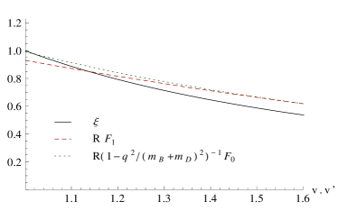
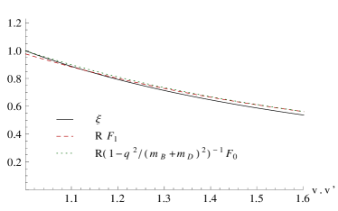
Figure 6: (Color online) Weak $B^{-}\rightarrow D^{0}$ decay form factors (multiplied with appropriate kinematical factors, cf. Eqs. (89) - (91)) for physical heavy-quark masses in comparison with the Isgur-Wise function (left figure). Model parameters are the same as in Fig. 2. In the right figure $c$ and $b$-quark masses are multiplied by a factor $6.25$ such that $m_{c}=10$ GeV and meson masses are taken equal to the corresponding quark masses.

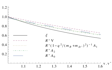
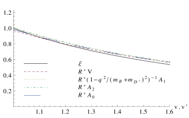
Figure 7: (Color online) Weak $B^{-}\rightarrow D^{0\ast}$ decay form factors (multiplied with appropriate kinematical factors, cf. Eqs. (94) - (97)) for physical heavy-quark masses in comparison with the Isgur-Wise function (left figure). Model parameters are the same as in Fig. 2. In the right figure $c$ and $b$-quark masses are multiplied by a factor $6.25$ such that $m_{c}=10$ GeV and meson masses are taken equal to the corresponding quark masses.

As we have discussed already in Sec. III.1, wrong cluster properties inherent in the Bakamjian-Thomas construction may lead to an unwanted dependence of the electromagnetic form factors on Mandelstam-$s$. Note that such an $s$-dependence does not spoil the Poincaré invariance of our $1$-photon-exchange amplitude, it rather hints at a non-locality of our photon-meson vertex. If one does not consider the full electron-meson scattering process, but rather the $\gamma^{\ast}M\rightarrow M$ subprocess, the $s$-dependence may be reinterpreted as a frame-dependence of our description of this subprocess. The two extreme cases are minimum $s$ to reach a particular momentum transfer $Q^{2}$ and $s\rightarrow\infty$ ($Q^{2}$ fixed). The first corresponds to the Breit frame, the latter to the infinite-momentum frame of the meson, respectively. In both cases the Lorentz structure of the electromagnetic current of a pseudoscalar meson may be expressed in terms of the physical covariant $(\underline{p}_{\alpha}+\underline{p}_{\alpha}^{\prime})^{\mu}$ alone and no spurious covariant or form factor is needed. The dashed and dotted lines in Fig. 5 show the electromagnetic form factors of the $D^{+}$ and $B^{-}$ mesons for $s\rightarrow\infty$ (infinite-momentum frame) and $s=m_{\alpha}^{2}+m_{e}^{2}+Q^{2}/2+2\sqrt{m_{\alpha}^{2}+Q^{2}/4}\sqrt{m_{e}^{2}+Q^{2}/4}$ (Breit frame), respectively. The differences are already rather small for the $D^{+}$ meson, become even smaller for the $B^{-}$ meson and vanish in the heavy-quark limit, as we have shown analytically in Sec. IV.1.

Semileptonic decays, involving time-like momentum transfers, are easier to handle. The decay currents that follow from our coupled channel approach can be expanded in terms of physical covariants alone and the form factors depend only on the 4-momentum transfer squared (cf. Sec. III.2). Plotted in Fig. 6 (left) are the two transition form factors that can be measured in the weak $B^{-}\rightarrow D^{0}e^{-}\bar{\nu}_{e}$ decay. These form factors are multiplied with appropriate kinematical factors such that they go over into the Isgur-Wise function when taking the heavy-quark limit. One prediction of heavy-quark symmetry is the approximate equality of $RF_{1}$ and $R(1-q^{2}/(m_{B}+m_{D})^{2})F_{0}$. For physical masses of the heavy quarks the differences are indeed less than $7\%$ of the absolute values of the form factors and tend to become smaller with increasing $\underline{v}\cdot\underline{v}^{\prime}$. Similar to the case of the space-like form factor of the $B^{-}$ meson the deviation from the Isgur-Wise function is still about $15\%$. In order to demonstrate numerically that $RF_{1}$ and $R(1-q^{2}/(m_{B}+m_{D})^{2})F_{0}$ converge to the Isgur-Wise function in the heavy-quark limit, we have made a calculation with $b$- and $c$-quark masses that are $6.25$ times larger than the physical masses (such that $m_{c}=10$ GeV). The result is shown in the right plot of Fig. 6. For such large masses of the heavy quark the discrepancy between $RF_{1}$, $R(1-q^{2}/(m_{B}+m_{D})^{2})F_{0}$ and $\xi$ shrinks already to less than $10\%$. A quantity that is often quoted is the slope of the Isgur-Wise function at zero recoil, $\rho^{2}=-\xi^{\prime}(1)$. For our simple wave function model we we have found $\rho^{2}=-\xi^{\prime}(1)=1.24$. This should be compared with the slope of $F_{D}(w)=RF_{1}(q^{2}(w))$ at zero recoil, $w=\underline{v}\cdot\underline{v}^{\prime}=1$, a quantity which is directly related to the (unpolarized) semileptonic decay rate, $d\Gamma_{B\rightarrow De\bar{\nu}}/dw\propto(w^{2}-1)^{3/2}|F_{D}(w)|^{2}$ Neubert (1994). In our case we get $F_{D}(1)=0.93$ and $\rho^{2}_{D}:=-F_{D}^{\prime}(1)/F_{D}(1)=0.59$, i.e. a considerably smaller slope than one would get in the heavy-quark limit. The up to date experimental value for the slope, as quoted by the Heavy Flavor Averaging Group Asner et al. (2010), is $\rho^{2}_{D}=1.18\pm 0.06$. Combining the results for the electromagnetic form factor of the $B^{-}$-meson in the space-like region and for the weak $B^{-}\rightarrow D^{0}$ decay form factors in the time-like region one can say that the breaking of heavy-quark flavor symmetry due to the finite masses of the heavy quarks is at most a $15-20\%$ effect.

Similar quantitative conclusions can be drawn for the breaking of heavy quark spin symmetry from the comparison of the weak $B^{-}\rightarrow D^{0\ast}$ decay form factors amongst each other and with the Isgur-Wise function. Heavy-quark symmetry predicts that $R^{\ast}V$, $R^{\ast}A_{0}$, $R^{\ast}A_{2}$, and $R^{\ast}(1-q^{2}/(m_{B}+m_{D})^{2})A_{1}$ should coincide in the heavy-quark limit. The maximum difference is again about $5\%$ of the absolute value, whereas the maximum deviation from the Isgur-Wise function is about $20\%$, such that breaking of heavy-quark spin symmetry for physical quark masses in $B^{-}\rightarrow D^{0\ast}e^{-}\bar{\nu}_{e}$ amounts also to about $20\%$. The right plot in Fig. 7 shows how heavy-quark spin-symmetry is approximately restored if $b$- and $c$-quark masses are increased by about one order of magnitude.

At the end of this section we want to stress that our discussion of heavy-quark-symmetry breaking was restricted to effects that come from the finite mass of the heavy quarks. We have ignored effects that result from a (heavy) flavor dependence of the $B$- and $D^{(\ast)}$-meson wave functions, which would show up in more sophisticated constituent-quark models for heavy-light mesons. With a smaller oscillator parameter for the $D$-meson, as it is suggested in a front form analysis of heavy-meson decay constants Hwang (2010), one could, e.g., come closer to the experimental value for $\rho^{2}_{D}$.

VI Conclusions

In this paper we have extended and generalized previous work on the electromagnetic structure of spin-0 and spin-1 two-body bound states consisting of equal-mass particles Biernat et al. (2009); Biernat (2011); Biernat et al. (2011). Working within the point form of relativistic quantum mechanics and using a constituent-quark model with instantaneous confining force we have derived electroweak current matrix elements and (transition) form factors for heavy-light mesons in the space- and time-like momentum-transfer regions. Starting point of this derivation is a multichannel formulation of the physical processes in which these form factors are measured, i.e electron-meson scattering and semileptonic weak decays. This formulation accounts fully for the dynamics of the exchanged gauge boson ($\gamma$ or $W$). Poincaré invariance is guaranteed by adopting the Bakamjian-Thomas construction with gauge-boson-fermion vertices taken from quantum field theory. Vector and axial-vector currents of the mesons can then be uniquely identified from the one-boson-exchange ($\gamma$ or $W$) amplitudes. These currents have already the right Lorentz-covariance properties and the electromagnetic current of any pseudoscalar meson is conserved. But wrong cluster properties, inherent in the Bakamjian-Thomas construction Keister and Polyzou (1991), give rise to spurious dependencies of the electromagnetic current on the electron momenta. For pseudoscalar mesons this unwanted dependencies are eliminated by taking the invariant mass of the electron-meson system large enough Biernat et al. (2009); Biernat (2011); Biernat et al. (2011). The resulting electromagnetic form factor of a pseudoscalar meson is then equivalent to the one obtained in front form from the $+$-component of a one-body current in a $q^{+}=0$ frame. The weak pseudoscalar $\rightarrow$ pseudoscalar and pseudoscalar $\rightarrow$ vector transition currents are not plagued by such spurious contributions. They can be expressed in terms of physical covariants and form factors with the form factors depending on the (time-like) momentum transfer squared, as it should be. In front form one observes some frame dependence of the $B\rightarrow D^{\ast}$ decay form factors if they are extracted from the $+$-component of a simple one-body current Cheng et al. (1997). This is attributed to a missing non-valence (Z-graph) contribution, which makes the triangle diagram, from which the form factors are calculated, covariant Cheng et al. (1997); Bakker et al. (2003). In the case of the point form it is, of course, also not excluded that $Z$-graphs may play a role, but they are not necessary to ensure covariance of the current, since Lorentz boosts are purely kinematical and thus do not mix in higher Fock states.

Having derived comparably simple analytical expressions for the electromagnetic form factor of a pseudoscalar heavy-light meson and the $B\rightarrow D^{(\ast)}$ decay form factors we discussed the heavy-quark limit. We found that the decay form factors (multiplied with appropriate kinematical factors) go over into one universal function, the Isgur-Wise function, as demanded by heavy-quark symmetry. For the electromagnetic form factor we observed that the heavy-quark limit does not completely remove the spurious dependence on the electron momentum. One still has a spurious covariant and the $s$-dependence of the form factors goes over into a dependence on the (common) modulus of the incoming and outgoing 3-velocities of the heavy meson. This dependence on the modulus of the meson velocities vanishes by taking it large enough. In the limit of infinitely large meson velocities we found a rather simple analytical expression for the Isgur-Wise function which turned out to be (apart of a change of integration variables) the same as the expression which we got from the decay form factors. Interestingly, we have also got the same result for the Isgur-Wise function for the minimum value of the meson velocities that is necessary to reach a particular value of $\underline{v}\cdot\underline{v}^{\prime}$ (the argument of the Isgur-Wise function). For minimum velocities it is not possible to separate physical and spurious contributions since the respective covariants become proportional. The dependence of the electromagnetic pseudoscalar meson form factor on Mandelstam-$s$ and the dependence of the resulting Isgur-Wise function on the modulus of the meson velocities may be interpreted as a frame dependence of the $\gamma^{\ast}M\rightarrow M$ subprocess. The $s\rightarrow\infty$ (velocities $\rightarrow\infty$) limit corresponds to the infinite-momentum frame, whereas minimum $s$ (minimum velocities) corresponds to the Breit frame. Our finding thus means that it does not matter whether we calculate the Isgur-Wise function in the infinite-momentum frame or the Breit frame. In the heavy-quark limit the results are the same and agree with the heavy-quark limit of the decay form factors. Numerical agreement was also found with the front-form calculation of Ref. Cheng et al. (1997).

As a first application and numerical check of our approach we have calculated electromagnetic $D^{+}$- and $B^{-}$ form factors, the $B\rightarrow D^{(\ast)}$ decay form factors and the Isgur-Wise function with a simple (flavor independent) Gaussian wave function. For the electromagnetic $B^{-}$ form factor and for the $B\rightarrow D^{(\ast)}$ decay form factors the effect of heavy-quark symmetry breaking due to finite physical masses of the heavy quarks turned out be $15-20\%$. For the electromagnetic $D^{+}$ form factor it rather amounted to about $60\%$.

To conclude, we have presented a relativistic point-form formalism for the calculation of the electroweak structure of heavy-light mesons within constituent quark models with instantaneous confining forces. This formalism provides the electromagnetic form factor of pseudoscalar heavy-light systems for space-like momentum transfers and weak pseudoscalar-to-pseudoscalar as well as pseudoscalar-to-vector decay form factors for time like momentum transfers. It exhibits the correct heavy-quark-symmetry properties in the heavy-quark limit. Although we have not presented results, our approach is immediately applicable to semileptonic heavy-to-light transitions and it is general enough to deal with additional dynamical degrees of freedom, such that one could, e.g., account for non-valence Fock-state contributions in the mesons Kleinhappel and Schweiger (2011).