Abstract

We study a model of directed polymers in random environment in dimension $1+d$, given by a Brownian motion in a Poissonian potential. We study the effect of the density and the strength of inhomogeneities, respectively the intensity parameter $\nu$ of the Poisson field and the temperature inverse $\beta$. Our results are: (i) fine information on the phase diagram, with quantitative estimates on the critical curve; (ii) pathwise localization at low temperature and/or large density; (iii) complete localization in a favourite corridor for large $\nu\beta^{2}$ and bounded $\beta$.

Short Title: Brownian Polymers

Key words and phrases: Directed polymers, random environment

AMS 1991 subject classifications: Primary 60K37; secondary 60Hxx, 82A51, 82D30

1 Introduction

We study in the present article the long-time behavior of the Brownian directed polymer in dimension $d\geq 1$, under the influence of a random Poissonian environment, as introduced in [10]. Let $B=(B_{t})_{t\geq 0}$ be the canonical Brownian motion in ${\mathbb{R}}^{d}$ starting at the origin, and $P$ the Wiener measure. Let also $Q$ be the law of the canonical Poisson point process $\eta$ in ${\mathbb{R}}_{+}\times{\mathbb{R}}^{d}$ with intensity measure $\nu dtdx$, where $\nu$ is a positive parameter. Denote by $U(x)\subset{\mathbb{R}}^{d}$ the closed ball with the unit volume, centered at $x\in{\mathbb{R}}^{d}$, and by

$$H_{t}^{\eta}(B)={\rm Card}\left\{{\rm points}\;(s,x)\;{\rm in\ }\eta:s\leq t,\;x\in U(B_{s})\right\},$$

the number of Poisson points which are ”seen” by the path $B$ up to time $t$. We are interested in the behavior of $B$ for large $t$ and typical $\eta$, under the polymer measure $\mu_{t}$ on the path space $C({\mathbb{R}}_{+}\rightarrow{\mathbb{R}}^{d})$ given by

$$d\mu_{t}=\frac{1}{Z_{t}}\exp\{\beta H_{t}^{\eta}(B)\}\;dP$$ (1.1)

Here, $Z_{t}$ is the normalizing constant, and $\beta\in{\mathbb{R}}$ is a parameter. Its absolute value, being proportional to the temperature inverse, measures the strength of the inhomogeneities produced by the random environment, whereas its sign indicates whether the path prefer to visit Poisson points or to stay clear from them. The model has an interpretation in terms of branching Brownian motions in random environment. When $\beta>0$, the Poisson points are catalyzers, and every point $(s,x)$ in $\eta$ causes an instantaneous (possibly multiple) branching with mean offspring $e^{\beta}$ to every individual passing by $x$ within distance $r_{d}$ at time $s$. When $\beta<0$, the Poisson points are soft obstacles, and every point $(s,x)$ in $\eta$ kills individual passing by $x$ within distance $r_{d}$ at time $s$ with probability $1-e^{\beta}$. Then, $Z_{t}$ is the average population at time $t$ in the environment $\eta$, e.g., the survival probability when $\beta\leq 0$, and the restriction of $\mu_{t}$ to time interval $[0,t]$ is the law of the ancestral line of a randomly selected individual in the population at time $t$, conditionally on survival.

This particular model was considered in [10, 11] with $\nu=1$. As is the rule for general polymer models, a salient feature in dimension $d\geq 3$, is a phase transition between a high temperature phase ($|\beta|$ small) where inhomogeneities are inessential, and a low temperature phase ($|\beta|$ large) where inhomogeneities are crucial. The phases are first defined by thermodynamic functions, namely by the dis/agreement of the quenched and annealed free energies, but it was discovered that they correspond to delocalized and localized behavior respectively, see [7, 9] for simpler models. The thermodynamic transition coincides with localization transition. The counterpart of the diffusive and of localized behaviors for branching Brownian motions have been studied in [33, 34] with a particular dynamics.

The proof that there exists a high temperature phase goes back to [22, 5]. The sub-region defined by the condition in (2.13) below, is called the $L^{2}$-region, is where $Z_{t}/QZ_{t}$ is bounded in $L^{2}$. There, second moment method works, showing that the polymer measure is much similar to the Wiener measure. Non perturbative results covering the full high temperature region are rare.

At low temperature, localization properties are traditionally formulated for the end point of the polymer as in [7, 9]. Recent results in [8] for the parabolic Anderson model, have led to substantial progress in understanding that localization holds in a stronger, pathwise manner there: The polymer path spends a positive proportion of time at the same location as some particular path depending on the realization of the medium. The proof crucially uses the Gaussian nature of the environment, via integration by parts formula, and it is not clear how general pathwise localization is. We observe that the concentration effect is a global phenomenon in our model, in contrast with heavy-tails potentials where only extreme statistics are relevant [2, 20] and it only matters that the random path visits the few corresponding locations. By nature, available information in the present model concerns replica overlaps. Moments, covariances, conditional moments can often be represented as expected values of independent copies of the paths sharing the same environment, so-called replica. A necessary step is to extract, from the latter, information on a single polymer.

The present model is quite natural, and interestingly enough, it is related to other polymer models. For instance, the mean field limit, $\nu\to\infty$ and $\beta\to 0$ in such a way that $\nu\beta^{2}\to b^{2}>0$, is the Brownian directed polymer in a Gaussian environment. In this model introduced in [31], the environment is the generalized Gaussian process $g(t,x)$ with mean 0 and covariance

$$Q[g(t,x)g(s,y)]=b^{2}\delta(t-s)|U(x)\cap U(y)|,$$

where $|\;\cdot\;|$ above denotes the Lebesgue measure. As mentioned in [26], the proofs of superdiffusivity in one space dimension and the analysis of the influence of spatial correlations for the Gaussian environment case, can be adapted to our case of a Poissonian environment.

A few exactly solvable polymer models are known so far, all of them being for $d=1$: (i) the infinite series of Brownian queues [30, 28], which is a limit of strongly asymmetric polymers [27]; (ii) the discrete model with log-gamma weights [32, 15]; (iii) the Hopf-Cole solution of the one-dimensional Kardar-Parisi-Zhang equation [1], which is expected the universal scaling limit for polymers [12]. Exact solutions are also available at zero temperature, via determinantal processes. Note that, from [25], there is no high temperature region in dimension $d=1$ and $2$.

For disordered polymer pinning on an interface, which also shows localized and a delocalized phases, estimating the critical curve is an important and difficult problem [16, 21]. The similar remark also holds for bulk disorder with long range correlation [6]. Unrelated disordered systems, including the Sherrington-Kirkpatrick model, have seen the emergence of smart interpolation techniques [38, 18, 19], allowing to compare the free energy with that of an auxiliary, simpler model.

We finally mention the relations to the non directed, model of Brownian motion in a space-dependent (but time independent) Poissonian potential, which has been extensively studied in many different perspectives; We refer to [37] for a detailed overview. The spectral theory approach and the coarse-graining method of enlargement of obstacles developed in [37] does not apply to our directed model. The latter one can be thought as the case of very strong drift in a fixed direction, or, equivalently, the problem of long crossings, which has been considered in such continuous models [40] as well as in discrete ones [23, 41].

The main objective of the present paper is to study the joint effect of the density and the strength of inhomogeneities, i.e., the influence of the intensity parameter $\nu$ and of the temperature inverse $\beta$. We obtain qualitative and quantitative estimates on the critical curve separing the two phases in the plane $(\beta,\nu)$. We find some auxiliary curves in this plane along which the difference between the annealed and quenched free energies is monotone, thus they do not re-enter a phase after leaving. In the spirit of the interpolation techniques mentioned above, the control of the sign of the derivative is made possible in the present model by the integration by parts formula for the Poisson process. A second set of results is for the pathwise localization in the localized phase, it applies in all space dimension $d=1,2\ldots$ (the polymer ”physical” dimension being $1+d$). We define a trajectory – we call it the favourite path for obvious reasons – depending on the realization of the medium and on the parameters, in the vicinity of which the random polymer path spends a positive fraction of time. Moreover, the localization in the favourite corridor becomes complete in some region of the parameter space: we show that this fraction converges to 1 as $\nu\beta^{2}\to\infty$ with $\beta$ remaining bounded. To parallel the notion of geodesics in last passage percolation [29], the favourite path can be viewed as a ”fuzzy geodesics”, and this one is essentially unique in this asymptotics.

Our paper is organized as follows: We start with notations and previous results. We then formulate our main results in section 3. In the next section we define the favourite path, the overlap between two polymer paths (replica), and prove a ”two-to-one lemma”, which extracts information on a single polymer path from the overlap of two replica. Section 5 contains the proofs of localization, except for an estimate, needed for complete localization, of the discrepancy of quenched and annealed free energies, which is obtained in section 6. The final section is devoted to the estimates of the critical curve.

2 The model of Brownian directed polymers in random environment

2.1 Preliminaries

We set some more notations. The environment $\eta$ is the Poisson random measure on ${\mathbb{R}}_{+}\times{\mathbb{R}}^{d}$ with the intensity $\nu>0$, defined on the probability space $({\cal M},{\cal G},Q)$, with ${\cal M}$ is the set of integer-valued Radon measure on ${\mathbb{R}}_{+}\times{\mathbb{R}}^{d}$, ${\cal G}$ is the $\sigma$-field generated by the variables $\eta(A)\;,\;A\in{\cal B}({\mathbb{R}}_{+}\times{\mathbb{R}}^{d})$. $Q$ is the unique probability measure on $({\cal M},{\cal G})$ such that, for disjoint and bounded $A_{1},...,A_{n}\in{\cal B}({\mathbb{R}}_{+}\times{\mathbb{R}}^{d})$, the variables $\eta(A_{j})$ are independent with Poisson distribution of mean $\nu|A_{j}|$; Here, $|\cdot|$ denotes the Lebesgue measure on ${\mathbb{R}}^{1+d}$. For $t>0$, it is natural and convenient to introduce its restriction

$$\eta_{t}(A)=\eta(A\cap((0,t]\!\times\!{\mathbb{R}}^{d}))\;,\;\;\;A\in{\cal B}({\mathbb{R}}_{+}\times{\mathbb{R}}^{d}).$$ (2.1)

We denote by $V_{t}$ the tube around the graph $\{(s,B_{s})\}_{0<s\leq t}$ of the Brownian path,

$$V_{t}=V_{t}(B)=\{(s,x)\;;\;s\in(0,t],\;x\in U(B_{s})\},$$ (2.2)

where $U(x)\subset{\mathbb{R}}^{d}$ is the closed ball with the unit volume, centered at $x\in{\mathbb{R}}^{d}$. ($U(x)$ has radius $r_{d}$.) Then, for any $t>0$, the polymer measure $\mu_{t}^{x}$ can be expressed as

$$d\mu_{t}={(Z_{t})^{-1}}{\exp\left(\beta\eta(V_{t})\right)}\;dP,$$ (2.3)

with the partition function $Z_{t}$

$$Z_{t}=P[\exp\left(\beta\eta(V_{t})\right)]\;.$$ (2.4)

Let $f,g:I\rightarrow(0,\infty)$ be functions and $a\in\overline{I}$, where $I\subset{\mathbb{R}}$ is an interval. We write $f(x)\sim g(x)$ ($x\rightarrow a$), if $\lim_{x\rightarrow a}f(x)/g(x)=1$. We write $f(x)\asymp g(x)$ ($x\rightarrow a$), if $0<\mathop{\underline{\lim}}_{x\rightarrow a}f(x)/g(x)\leq\mathop{\overline{\lim}}_{x\rightarrow a}f(x)/g(x)<\infty$.

2.2 Former results

Denote by $\lambda$ the logarithmic moment generating function of a mean-one Poisson distribution,

$$\lambda=\lambda(\beta)=e^{\beta}-1\in(-1,\infty)\;.$$ (2.5)

The quenched free energy $p_{t}(\beta,\nu)$ of the polymer model with finite time horizon $t$ is

$$p_{t}(\beta,\nu)=\frac{1}{t}Q\ln Z_{t},$$ (2.6)

though $\frac{1}{t}\ln QZ_{t}=\nu\lambda(\beta)$ is the annealed free energy. The case of a fixed $\nu=1$ was considered in the papers [10, 11], but the results trivially extend to a general $\nu$. We summarize them without repeating the proof.

Theorem 2.2.1

Let $d\geq 1,\nu>0$ and $\beta\in{\mathbb{R}}$ be arbitrary.

(a)

There exists a deterministic number $p(\beta,\nu)\in{\mathbb{R}}$ such that

$$p(\beta,\nu) = \lim_{t\nearrow\infty}p_{t}(\beta,\nu),$$ (2.7)

$$= \lim_{t\nearrow\infty}\frac{1}{t}\ln Z_{t},\;\;\;\mbox{$Q$-a.s. and in $L^{2}(Q)$.}$$ (2.8)

(b)

The function $\beta\mapsto p(\beta,\nu)$ is convex on ${\mathbb{R}}$, with

$$\nu\beta\leq p(\beta,\nu)\leq\nu\lambda.$$ (2.9)

The function $\beta\mapsto\nu\lambda(\beta)-p(\beta,\nu)$ is non-decreasing on ${\mathbb{R}}_{+}$ and non-increasing on ${\mathbb{R}}_{-}$.

(c)

There exist critical values $\beta_{c}^{\pm}=\beta_{c}^{\pm}(\nu)=\beta_{c}^{\pm}(d,\nu)$ with $-\infty\leq\beta^{-}_{c}\leq 0\leq\beta^{+}_{c}<+\infty,$ such that

$$p(\beta,\nu)=\nu\lambda\;\; \;\;\beta\in[\beta_{c}^{-},\beta^{+}_{c}]\cap{\mathbb{R}},$$ if (2.10)

$$p(\beta,\nu)<\nu\lambda,\;\; \;\;\beta\in{\mathbb{R}}\backslash[\beta_{c}^{-},\beta^{+}_{c}].$$ if (2.11)

(d)

For $d\geq 3$, $\beta^{-}_{c}(d,\nu)<0<\beta^{+}_{c}(d,\nu)$, ${\displaystyle\lim_{d\nearrow\infty}\beta_{c}^{\pm}(d,\nu)=\pm\infty}$, and there exists $\nu_{c}\in[1,\infty]$ (cf. Proposition 3.1.1 below) such that

$$\beta^{-}_{c}(d,\nu)\left\{\begin{array}[]{ll}=-\infty&\mbox{if $\nu<\nu_{c}$},\\ >-\infty&\mbox{if $\nu>\nu_{c}$}.\end{array}\right.$$ (2.12)

More precisely, letting

$$a_{L^{2}}=\sup\left\{a>0:P\Big{[}\exp\left({a\over 2}\int^{\infty}_{0}|U(0)\cap U(B_{s})|ds\right)\Big{]}<\infty\right\}>0,$$

then

$$\nu\lambda(\beta)^{2}<a_{L^{2}}\Longrightarrow p(\beta,\nu)=\nu\lambda(\beta)\;,$$ (2.13)

and thus, $\nu_{c}\geq a_{L^{2}}$ and

$$\beta^{-}_{c}(d,\nu)\leq\ln\left(1-\sqrt{a_{L^{2}}/\nu}\right)<\ln\left(1+\sqrt{a_{L^{2}}/\nu}\right)\leq\beta^{+}_{c}(d,\nu).$$ (2.14)

For completeness, we mention a numerical lower bound for $a_{L^{2}}$, and thus for $\nu_{c}$ itself, which can be derived from the techniques of section 4.2 in [10]. Let $\gamma_{d}$ denote the smallest positive zero of the Bessel function $J_{\frac{d-4}{2}}(\gamma)=(\gamma/2)^{{\frac{d-4}{2}}}\sum_{k\geq 0}{(-\gamma^{2}/4)^{k}}/({k!\Gamma({\frac{d-4}{2}}+k+1)}),$ $\gamma\geq 0.$ Then, with $r_{d}$ the radius of the ball $U(0)$ with unit volume,

$$\nu_{c}\geq\left(\frac{\gamma_{d}}{2r_{d}}\right)^{2}.$$ (2.15)

The lower bound has value 1.265…for $d=3$, 1.792…for $d=4$, 2.190…for $d=5$, and $\liminf_{d\to\infty}d^{-1/2}\nu_{c}\geq\sqrt{e/(8\pi)}=0.329\ldots$.

3 Main results

3.1 Phase diagram

The parameter space $(0,\infty)\times{\mathbb{R}}$ splits into two regions,

$${\cal D}=\{(\nu,\beta):p(\nu,\beta)=\nu\lambda(\beta)\},\qquad{\cal L}=\{(\nu,\beta):p(\nu,\beta)<\nu\lambda(\beta)\}={\cal D}^{c},$$

which are called high temperature / low density region and low temperature / high density region respectively. The name is justified by observing that infinite temperature, or equivalently, $\beta=0$, belongs to $\mathcal{D}$, though zero density $\nu=0$ belongs to this set. We already know from [10] that they correspond to end-point delocalized and localized phase, see (3.27) below. In the next section, we will discuss deeper aspects of localization.

We state some properties of ${\cal L},{\cal D}$, and of the critical curve separating the two sets,

$$\tt Crit={\cal D}\cap\overline{\cal L}.$$

It is proved in [3] that ${\cal D}$ reduces to the semi-axis $\{\nu>0,\beta=0\}$ in dimensions $d=1$ and $d=2$, so we focus on the case of a larger dimension. By Theorem 2.2.1 , (2.10), (2.11), we already know that $\tt Crit$ is the union of the graphs of the functions $\nu\mapsto\beta_{c}^{-}(d,\nu)$ and $\nu\mapsto\beta_{c}^{+}(d,\nu)$. Moreover, by Lemma 7.1.1 we see that $\nu\lambda(\beta)-p(\nu,\beta)$ is non-decreasing in $\nu$, non-decreasing in $\beta$ for $\beta\geq 0$ and non-increasing in $\beta$ for $\beta\leq 0$. The qualitative features of the phase diagram are summarized in figure 1, corresponding to statements all through the present Section 3.

We first answer some questions which were left open in Theorem 2.2.1, (e).

Proposition 3.1.1

For all dimension $d\geq 3$, we have

$$\nu_{c}<\infty$$ (3.1)

and

$$\beta_{c}^{-}(\nu_{c})=-\infty,$$ (3.2)

Recall for completeness that, in lower dimensions $d=1,2,$ we know from [3] that $\beta^{-}_{c}(\nu)=0$ for all $\nu$. We prove (3.1) as a part of Corollary 5.3.2 below. By (3.1), the set ${\cal D}$ contains North-West quadrants $[\nu^{\prime},\infty)\times(-\infty,\beta^{\prime}]$ with $\nu^{\prime}>\nu_{c},\beta^{\prime}<\beta_{c}^{-}((\nu_{c}+\nu^{\prime})/2)$. Once (3.1) is confirmed, (3.2) follows immediately from the definition of $\nu_{c}$ and the fact that ${\cal D}$ is a closed set.

3.2 Critical curves

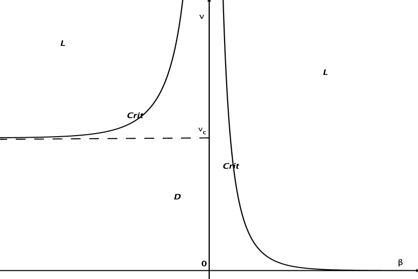
Figure 1: Phase diagram, $d\geq 3$. The high temperature/low density and low temperature/high density phases $\cal D$ and $\cal L$ are separated by the critical curve $\{(\beta_{c}^{+}(\nu),\nu);\nu>0\}\cup\{(\beta_{c}^{-}(\nu),\nu);\nu>\nu_{c}\}$

We introduce:

$$\alpha(\beta)={(e^{\beta}-1)^{2}\over e^{\beta}(e^{\beta}-1-\beta)},\;\;\;\beta\in{\mathbb{R}},\;\;\mbox{with $\alpha(0)\stackrel{{\scriptstyle\rm def.}}{{=}}2$.}$$ (3.3)

We note that

$$\alpha(\beta) \alpha(-\infty)=+\infty \alpha(\infty)=1$$ decreases from to . (3.4)

Our first main result consists in upper and lower bounds on the critical values $\beta^{\pm}_{c}(\nu)$. The following estimates show in particular that $\beta^{+}_{c}(\nu)$ (resp. $\beta^{-}_{c}(\nu)$) is locally Lipschitz continuous and strictly decreasing (resp. increasing) in $\nu$.

Theorem 3.2.1

Let $d\geq 3$.

(a1)

If $0<\nu_{0}<\nu$ and $1\leq\alpha\leq\alpha(\beta^{+}_{c}(\nu_{0}))$, then,

$$\ln\left(1+c_{1}^{+}(\nu_{0})\left(\nu_{0}\over\nu\right)^{1/\alpha}\right)\leq\beta^{+}_{c}(\nu)\leq\ln\left(1+c_{1}^{+}(\nu_{0})\left(\nu_{0}\over\nu\right)^{1/2}\right),$$ (3.5)

$$c_{2}^{+}(\nu_{0})\left(1-\left(\nu_{0}\over\nu\right)^{1/2}\right)\leq\beta^{+}_{c}(\nu_{0})-\beta^{+}_{c}(\nu)\leq c_{2}^{+}(\nu_{0})\left(\left(\nu\over\nu_{0}\right)^{1/\alpha}-1\right),$$ (3.6)

where $c_{1}^{+}(\nu_{0})=\lambda(\beta^{+}_{c}(\nu_{0}))$ and $c_{2}^{+}(\nu_{0})=1-\exp(-\beta^{+}_{c}(\nu_{0}))$.

(a2)

If $0<\nu_{1}\leq\nu<\nu_{0}$ and $1\leq\alpha\leq\alpha(\beta^{+}_{c}(\nu_{1}))$, then,

$$\ln\left(1+c_{1}^{+}(\nu_{0})\left(\nu_{0}\over\nu\right)^{1/2}\right)\leq\beta^{+}_{c}(\nu)\leq\ln\left(1+c_{1}^{+}(\nu_{0})\left(\nu_{0}\over\nu\right)^{1/\alpha}\right),$$ (3.7)

$$c_{2}^{+}(\nu_{0})\left(1-\left(\nu\over\nu_{0}\right)^{1/2}\right)\leq\beta^{+}_{c}(\nu)-\beta^{+}_{c}(\nu_{0})\leq c_{2}^{+}(\nu_{0})\left(\left(\nu_{0}\over\nu\right)^{1/\alpha}-1\right).$$ (3.8)

(b1)

If $\nu_{c}<\nu_{0}<\nu$ (cf. (2.12)) and $\alpha(\beta^{-}_{c}(\nu_{0}))\leq\alpha$, then,

$$\ln\left(1-c_{1}^{-}(\nu_{0})\left(\nu_{0}\over\nu\right)^{1/\alpha}\right)\leq\beta^{-}_{c}(\nu)\leq\ln\left(1-c_{1}^{-}(\nu_{0})\left(\nu_{0}\over\nu\right)^{1/2}\right),$$ (3.9)

$$c_{2}^{-}(\nu_{0})\left(1-\left(\nu_{0}\over\nu\right)^{1/\alpha}\right)\leq\beta^{-}_{c}(\nu)-\beta^{-}_{c}(\nu_{0})\leq c_{2}^{-}(\nu_{0})\left(\left(\nu\over\nu_{0}\right)^{1/2}-1\right),$$ (3.10)

where $c_{1}^{-}(\nu_{0})=|\lambda(\beta^{-}_{c}(\nu_{0}))|$ and $c_{2}^{-}(\nu_{0})=\exp(-\beta^{-}_{c}(\nu_{0}))-1$.

(b2)

If $\nu_{c}<\nu_{1}\stackrel{{\scriptstyle\rm def}}{{=}}\nu_{0}c_{2}^{-}(\nu_{0})^{2}<\nu<\nu_{0}$ and $\alpha\geq\alpha(\beta^{-}_{c}(\nu_{1}))$, then,

$$\ln\left(1-c_{1}^{-}(\nu_{0})\left(\nu_{0}\over\nu\right)^{1/2}\right)\leq\beta^{-}_{c}(\nu)\leq\ln\left(1-c_{1}^{-}(\nu_{0})\left(\nu_{0}\over\nu\right)^{1/\alpha}\right),$$ (3.11)

$$c_{2}^{-}(\nu_{0})\left(\left(\nu_{0}\over\nu\right)^{1/\alpha}-1\right)\leq\beta^{-}_{c}(\nu_{0})-\beta^{-}_{c}(\nu)\leq c_{2}^{-}(\nu_{0})\left(1-\left(\nu\over\nu_{0}\right)^{1/2}\right).$$ (3.12)

The proof of Theorem 3.2.1 will be presented in section 7.1. From the above estimates we derive the following quantitative informations. The first one follows from (3.7) with $\nu=\nu_{1}$ and $\alpha=1$, and the second one is from Corollary 5.3.2:

Corollary 3.2.2

For $d\geq 3$, we have

$$\beta^{+}_{c}(d,\nu)\asymp\ln(1/\nu)\;\;\mbox{as $\nu\searrow 0$},$$ (3.13)

and also,

$$|\beta^{\pm}_{c}(d,\nu)|\asymp 1/\sqrt{\nu}\quad{\rm as}\quad\nu\nearrow\infty.$$ (3.14)

Remark 3.2.3

In dimension $d\geq 3$, a phase transition occurs on the curve $\tt Crit$. The function $p(\beta,\nu)$, being equal to the analytic function $\nu\lambda(\beta)$ on one side of the curve, takes a different value on the other side. We do not know what is the order of the phase transition. However, we will show that, when $d\geq 3$, the gradient of $p_{t}(\beta,\nu)$ converges as $t\to\infty$ to that of the limit $\nu\lambda(\beta)$, at all points of ${\cal D}$, in particular those in $\tt Crit$ (See the argument at the end of section 7.2).

3.3 Path localization

For all $t>0$ we define, in Proposition 4.1.1 below, a measurable function $(s,\eta)\mapsto{\mathsf{Y}}^{(t)}(s)$ with values in ${\mathbb{R}}^{d}$ such that

$$\mu_{t}\big{(}B_{s}\in U({\mathsf{Y}}^{(t)}(s))\big{)}=\max_{x\in{\mathbb{R}}^{d}}\mu_{t}\big{(}B_{s}\in U(x)\big{)},\qquad s\in[0,t].$$ (3.15)

${\mathsf{Y}}^{(t)}$ depends on the environment $\eta$, it is not continuous in general, however we call it the ”optimal path” or ”favorite path”. It is convenient to introduce the notation

$$\chi_{s,x}={\mathbf{1}}_{B_{s}\in U(x)}$$

for the indicator function that the path sees the point $(s,x)$, so that $\chi_{s,x}=\chi_{s,x}(B)={\mathbf{1}}_{V_{t}}(s,x)$, and

$$\eta(V_{t})=\int\chi_{s,x}\eta_{t}(ds,dx).$$

We define the overlap between two replicas $B$ and $\tilde{B}$, which plays a major role in quantitative estimates for localization:

$$R_{t}=R_{t}(B,\tilde{B})=\frac{1}{t}|V_{t}(B)\cap V_{t}(\tilde{B})|$$ (3.16)

and the overlap between a polymer path and the optimal path,

$$R^{*}_{t}=R^{*}_{t}(B,\eta)=\frac{1}{t}\int_{0}^{t}{\mathbf{1}}_{\{B_{s}\in U({\mathsf{Y}}^{(t)}(s))\}}ds.$$ (3.17)

Note that $R,R^{*}$ take values in the interval $[0,1]$, that

$$\mu_{t}^{\otimes 2}(R_{t})=\frac{1}{t}\int_{0}^{t}ds\int_{{\mathbb{R}}^{d}}\mu_{t}(\chi_{s,x})^{2}dx,$$ (3.18)

by Fubini’s theorem, and

$$\mu_{t}(R^{*}_{t})=\frac{1}{t}\int_{0}^{t}\mu_{t}\left[\chi_{s,{\mathsf{Y}}^{(t)}(s)}\right]ds=\frac{1}{t}\int_{0}^{t}\max_{x}\mu_{t}\left[B_{s}\in U(x)\right]ds.$$ (3.19)

We say that $\beta>0$ [resp., $\beta<0$] is a point of increase of $\nu\lambda-p$ if $\nu\lambda(\beta^{\prime})-p(\beta^{\prime},\nu)>\nu\lambda(\beta)-p(\beta,\nu)$ for all $\beta^{\prime}>\beta$ [resp., $\beta^{\prime}<\beta$]. If $\beta>0$ is a point of increase for $\nu\lambda-p$, then necessarily $\beta\geq\beta^{+}_{c}$. By monotonicity in Theorem 2.2.1 (b), we already know that

$$\left({\partial p\over\partial\beta}\right)_{+}(\beta,\nu)\leq\nu\lambda^{\prime}(\beta)\;\;\;{\rm for\ }\beta\geq 0,\qquad\left({\partial p\over\partial\beta}\right)_{-}(\beta,\nu)\geq\nu\lambda^{\prime}(\beta)\;\;\;{\rm for\ }\beta\leq 0,$$ (3.20)

where $\left(\frac{\partial}{\partial\beta}\right)_{\!\!-}$ [resp., $\left(\frac{\partial}{\partial\beta}\right)_{\!\!+}$] denote the left [resp., right] derivative. For a fixed $\nu$, $\beta\mapsto p(\beta,\nu)$ is differentiable except for at most countably many $\beta$’s, and hence, $\left(\frac{\partial p}{\partial\beta}\right)_{\pm}(\beta,\nu)=\frac{\partial p}{\partial\beta}(\beta,\nu)$ except such $\beta$’s.

The following result, in particular (3.24) which is the punchline, shows that a localization properties of the polymer is equivalent to the strictness of the inequality (3.20), up to the exceptional non-differentiability of $p(\cdot,\nu)$.

Theorem 3.3.1

(a)

There exists $c=c(d)\in(0,1]$ such that

$$c\left(Q\mu_{t}\left(R^{*}_{t}\right)\right)^{2}\leq Q\mu_{t}^{\otimes 2}\left(R_{t}\right)\leq Q\mu_{t}\left(R^{*}_{t}\right).$$ (3.21)

(b)

For $\beta\neq 0$ and $\nu>0$, define

$$\delta_{\pm}(\beta,\nu)=(\nu\lambda)^{-1}\left(\nu\lambda^{\prime}(\beta)-\left(\frac{\partial p}{\partial\beta}\right)_{\pm}(\beta,\nu)\right)\geq 0\;,\;\;\;$$ (3.22)

(cf. (3.20)). Then,

$$\liminf_{t\to\infty}Q\mu_{t}^{\otimes 2}\left(R_{t}\right)\geq\left\{\begin{array}[]{ll}e^{-\beta}\delta_{+}(\beta,\nu)&\mbox{if $\beta>0$},\\ \delta_{-}(\beta,\nu)&\mbox{if $\beta<0$}.\end{array}\right.$$ (3.23)

In particular,

$$\liminf_{t\to\infty}Q\mu_{t}\left(R^{*}_{t}\right)\geq\liminf_{t\to\infty}Q\mu_{t}^{\otimes 2}\left(R_{t}\right)>0$$ (3.24)

whenever the inequality (3.20) is strict. Moreover,

$$\limsup_{t\to\infty}Q\mu_{t}^{\otimes 2}\left(R_{t}\right)\leq\left\{\begin{array}[]{ll}\delta_{-}(\beta,\nu)&\mbox{if $\beta>0$},\\ e^{|\beta|}\delta_{+}(\beta,\nu)&\mbox{if $\beta<0$}.\end{array}\right.$$ (3.25)

(c1)

For a fixed $\nu$, $\delta_{-}(\beta,\nu)\geq\delta_{+}(\beta,\nu)>0$ if $\beta>0$ is large enough.

(c2)

For all points $\beta$ of increase of $\nu\lambda-p(\cdot,\nu)$, there exists a sequence $(\beta_{k})_{k}$ converging to $\beta$ such that for all $k$, $p(\cdot,\nu)$ is differentiable at $\beta_{k}$ and $\delta_{+}(\beta_{k},\nu)=\delta_{-}(\beta_{k},\nu)>0$.

The proof of Theorem 3.3.1 will be presented in section 5.2. Such statements express the strong localization properties of the polymer. In particular, the time-average $(1/t)\int_{0}^{t}{\mathbf{1}}_{B_{s}\in U({\mathsf{Y}}^{(t)}(s))}ds$ is the time fraction the polymer spends with the favourite path. Under the strictness of the inequality (3.20), the time fraction is positive. For a benchmark, we recall that, for the free measure $P$, for all smooth path ${\mathsf{Y}}$ and all $\delta>0$, there exists a positive $C$ such that for large $t$,

$$P\left(\frac{1}{t}\int_{0}^{t}{\mathbf{1}}_{B_{s}\in U({\mathsf{Y}}(s))}ds\geq\delta\right)\leq\exp\{-Ct\}$$ (3.26)

(In fact, it is not difficult to see (3.26) for $Y\equiv 0$ by applying Donsker-Varadhan’s large deviations [14]. Then, one can use Girsanov transformation to extend (3.26) to the case of smooth path ${\mathsf{Y}}$.)

The results of Theorem 3.3.1 are to be compared with the results in [10], that we recall now. These ones only deal with end points, i.e., with the location of the polymer at the last moment it interacts with the medium. If $p(\nu,\beta)<\nu\lambda(\beta)$, we have by Theorem 2.3.2 and Remark 2.3.1 of [10] that

$$\liminf_{t\to\infty}\frac{1}{t}\int_{0}^{t}\max_{x\in{\mathbb{R}}^{d}}\mu_{s}(B(s)\in U(x))ds\geq\liminf_{t\to\infty}\frac{1}{t}\int_{0}^{t}\int_{{\mathbb{R}}^{d}}\mu_{s}(\chi_{s,x})^{2}dsdx>0,\;\;\;\mbox{$Q$-a.s.}$$ (3.27)

Note that ${\mathsf{Y}}^{(t)}(t)$ is a maximizer of $\mu_{t}(B(t)\in U(x))$. As in [8], we conjecture that the set where localization occurs, coincides with the full low temperature/high density region ${\cal L}$, where the quenched free energy is strictly smaller than the annealed one:

Conjecture 3.3.2

$$\Big{\{}(\nu,\beta):\mbox{The inequality (\ref{eq:conj}) is strict}\Big{\}}={\cal L}.$$

We now turn to complete path localization. In the region where $\nu\beta^{2}$ is large with $\beta$ bounded, the localization becomes strong in various aspects. First of all, the fraction of time $t^{-1}\int_{0}^{t}{\mathbf{1}}_{B_{s}\in U({\mathsf{Y}}^{(t)}(s))}ds$ that the polymer spends in the neighborhood of the favourite path tends to its maximum value 1. This behavior is in a sharp contrast with the benchmark mentioned above.

Theorem 3.3.3

(Complete localization 1) Let $\beta_{0}\in(0,\infty)$ be arbitrary. Then, as $|\beta|\leq\beta_{0}$ and $\nu\beta^{2}\rightarrow\infty$,

$$\liminf_{t\to\infty}Q\mu_{t}\left(R^{*}_{t}\right) \geq \liminf_{t\to\infty}Q\mu_{t}^{\otimes 2}\left(R_{t}\right)$$ (3.28)

$$= 1-{\cal O}\left((\nu\beta^{2})^{-1/6}\right).$$ (3.29)

In other words, for any bounded function $\beta(\nu)$ with $\nu\beta(\nu)^{2}\to\infty$ as $\nu\to\infty$, the limit $\ell(\beta,\nu)=\liminf_{t\to\infty}Q\mu_{t}\left(R^{*}_{t}\right)\in[0,1]$ converges to its maximal value,

$$\ell(\beta(\nu),\nu)\to 1,\quad\nu\to\infty.$$

Of course, the parameter $\beta$ can become small, but not too much, since no localization occurs if $\beta=0$. The proof of Theorem 3.3.3, together with that of Theorem 3.3.4 below, will be presented in section 5.3.

We next extract fine additional information on the geometric properties of the Gibbs measure. For $\delta\in(0,1/2)$ define the $(\delta,t)$-negligible set as

$${\cal N}_{\delta,t}^{\eta}=\Big{\{}(s,x)\in[0,t]\times{\mathbb{R}}^{d}:\mu_{t}(\chi_{s,x})\leq\delta\Big{\}},$$

and the $(\delta,t)$-predominant set as

$${\cal P}_{\delta,t}^{\eta}=\Big{\{}(s,x)\in[0,t]\times{\mathbb{R}}^{d}:\mu_{t}(\chi_{s,x})\geq 1-\delta\Big{\}}.$$

As suggested by the names, ${\cal N}_{\delta,t}^{\eta}$ is the set of space-time locations the polymer wants to stay away from, and ${\cal P}_{\delta,t}^{\eta}$ is the set of locations the polymer likes to visit. Both sets depend on the environment.

Theorem 3.3.4

(Complete localization 2) For all $0<\delta<1/2$, we have as $|\beta|\leq\beta_{0}$ and $\nu\beta^{2}\rightarrow\infty$,

$$\limsup_{t\to\infty}Q\frac{1}{t}\Big{|}({\cal N}_{\delta,t}^{\eta}\cup{\cal P}_{\delta,t}^{\eta})^{\complement}\Big{|}={\cal O}\left((\nu\beta^{2})^{-1/6}\right),$$ (3.30)

$$\limsup_{t\to\infty}Q\mu_{t}\left[\frac{1}{t}\Big{|}V_{t}(B)\bigcap{\cal N}_{\delta,t}^{\eta}\Big{|}\right]={\cal O}\left((\nu\beta^{2})^{-1/6}\right),$$ (3.31)

$$\limsup_{t\to\infty}Q\mu_{t}\left[\frac{1}{t}\Big{|}V_{t}(B)^{\complement}\bigcap{\cal P}_{\delta,t}^{\eta}\Big{|}\right]={\cal O}\left((\nu\beta^{2})^{-1/6}\right).$$ (3.32)

Recall that $|\cdot|$ denotes the Lebesgue measure on ${\mathbb{R}}_{+}\times{\mathbb{R}}^{d}$, and note that $|{\cal N}_{\delta,t}^{\eta}|=|V_{t}(B)^{\complement}|=\infty$.

The limits (3.30), (3.31), (3.32), bring information on how is the corridor around the favourite path where the measure concentrates for large $\nu\beta^{2}$. In this limit:

• most (in Lebesgue measure) time-space locations become negligible or predominant,

• most (in Lebesgue and Gibbs measures) negligible locations are outside the tube around the polymer path,

• most (in Lebesgue and Gibbs measures) predominant locations are inside the tube around the polymer path.

The trace $\big{\{}x\in{\mathbb{R}}^{d}:\mu_{t}(\chi_{s,x})\geq 1-\delta\big{\}}$ at time $t$ of the $(\delta,t)$-predominant set is reminiscent of the $\epsilon$-atoms discovered in the discrete setting in [39], with $\epsilon=1-\delta$.

4 Replica overlaps and favourite path

We build on ideas similar to [8]. Since the state space is continuous, some measurability issues appear, but also the geometric properties of the path measure are of interest.

4.1 Favourite path

For all times $s\leq t$, the function $x\mapsto\mu_{t}(B_{s}\in U(x))=\mu_{t}(\chi_{s,x})$ achieves its maximum, and the set of maximizers is compact. We want to consider ”the maximizer”, by selecting a specific element in the argmax in case of multiplicity, but this can be effective only with some measurability property. For a function $f:{\mathbb{R}}^{d}\to{\mathbb{R}}$ and a set $A\subset{\mathbb{R}}^{d}$, we denote by

$$\arg\max_{x\in A}f(x)=\{x\in A:f(x)=\sup_{z\in A}f(z)\}$$ (4.1)

the set of the maximizer of $f$ on $A$.

Proposition 4.1.1

There exists a measurable subset ${\cal M}^{0}\subset{\cal M}$, and for each fixed $t>0$, a measurable function

$$(s,\eta)\mapsto{\mathsf{Y}}^{(t)}(s):[0,t]\times{\cal M}^{0}\to{\mathbb{R}}^{d}$$

such that

$$Q({\cal M}^{0})=1 Z_{t}(\eta)<\infty \beta\in{\mathbb{R}} t>0 \eta\in{\cal M}^{0}$$ and for all , and , (4.2)

$${\mathsf{Y}}^{(t)}(s)\in\arg\max_{x\in{\mathbb{R}}^{d}}\mu_{t}\big{(}B_{s}\in U(x)\big{)}.$$ (4.3)

As indicated in the notation, we will regard ${\mathsf{Y}}^{(t)}(\cdot)$ as a function on $[0,t]$, which depends on $t$, but we keep in mind that it also depends on $\beta$ and on $\eta\in{\cal M}^{0}$. It is not continuous in general, however we call it the ”favourite path”.

Proof of Proposition 4.1.1: We recall that ${\cal M}$ is a Polish space under the vague topology ${\cal T}$ [24, p. 170, 15.7.7] and that the Borel $\sigma$-field $\sigma[{\cal T}]$ coincides with ${\cal G}$ [24, p. 32, Lemma 4.1]. This observation enables us to exploit a measurable selection theorem from [36, p.289, Theorem 12.1.10], as we explain now.

We start with the definition of ${\cal M}^{0}$. Let $r=r_{d}$ be the radius of $U(0)$ and

$$\widetilde{V}_{t}=\{(s,x)\in[0,t]\times{\mathbb{R}}^{d}\;;\;\exists u\geq 0,|u-s|\leq 1,|x-B_{u}|\leq r+1\}$$

be an enlargement of $V_{t}$. We define

$${\cal M}^{0}=\bigcap_{\beta,t>0}\left\{\eta\in{\cal M}\;;\;P\big{[}\exp(\beta\eta(\widetilde{V}_{t}))\big{]}<\infty\right\},$$ (4.4)

which satisfies (4.2). In the following argument, we always assume that $\eta\in{\cal M}^{0}$. With

$$Z_{t}(s,x,\eta)=P[\zeta_{t}(\eta);B_{s}\in U(x)],\;\;\;\zeta_{t}(\eta)=\exp\{\beta\eta(V_{t})\},$$

we can write the right-hand side of (4.3) as

$$\arg\max_{x\in{\mathbb{R}}^{d}}\mu_{t}\big{(}B_{s}\in U(x)\big{)}=\arg\max_{x\in{\mathbb{R}}^{d}}Z_{t}(s,x,\eta).$$

Thus, we wish to select a maximizer of $x\mapsto Z_{t}(s,x,\eta)$ as a measurable function in $(s,\eta)$. As can be seen below, our method relies heavily on the continuity of the functions we work with (cf. the proof of Lemma 4.1.2). Unfortunately, $Z_{t}(s,x,\eta)$ is discontinuous at all $(s,x,\eta)$ such that $\eta(\{s\}\times U(x))\geq 1$. To circumvent this obstacle, we will consider a continuous approximation of $Z_{t}(s,x,\eta)$ (cf. (4.5) below), together with a cut-off of $x$-variables. Let $\varphi:{\mathbb{R}}\to{\mathbb{R}}_{+}$ be continuous, supported inside $[-1,1]$, and the integral equal to one. For $k\geq 1$, let $\varphi^{(k)}(t)=k\varphi(kt)$, and $\psi^{(k)}(x)=\big{[}1-k\times{\rm dist}(x,U(0))\big{]}^{+}$. Then we have, as $k\to\infty$, $\varphi^{(k)}(t)dt\to\delta_{0}(dt)$ weakly, and $\psi^{(k)}\to{\mathbf{1}}_{U(0)}$ pointwise. Define

$$\zeta^{(k)}_{t}(\eta)=\exp\{\beta\int\eta_{t}(dsdx)\int_{\mathbb{R}}\varphi^{(k)}(s-u)\psi^{(k)}(B_{u}-x)du\},$$

and

$$Z^{(k)}_{t}(s,x,\eta)=P[\zeta^{(k)}_{t}(\eta);B_{s}\in U(x)].$$ (4.5)

Note that, with $u^{+}=\max\{u,0\}$,

$$\zeta^{(k)}_{t}(\eta)\leq\exp(\beta^{+}\eta(\widetilde{V}_{t+1})),$$ (4.6)

and hence $Z^{(k)}_{t}(s,x,\eta)<\infty$ for all $\eta\in{\cal M}^{0}$. Let ${\cal K}$ be the totality of compact subsets in ${\mathbb{R}}^{d}$, equipped with the Hausdorff metric. Then, we will show in Lemma 4.1.2 below that, for any integer $\ell\geq 1$, the mapping,

$$(s,\eta)\mapsto K^{(k,\ell)}(s,\eta)=\arg\max_{x\in[-\ell,\ell]^{d}}Z^{(k)}_{t}(s,x,\eta)$$ (4.7)

defined by (4.1), is Borel measurable from $[0,t]\times{\cal M}^{0}$ to ${\cal K}$. Thanks to this measurability, which we will assume for the moment, we deduce from the measurable selection theorem mentioned above, that there exists a measurable mapping ${\mathsf{Y}}^{(t,k,\ell)}:[0,t]\times{\cal M}^{0}\to[-\ell,\ell]^{d}$ such that

$${\mathsf{Y}}^{(t,k,\ell)}(s,\eta)\in K^{(k,\ell)}(s,\eta).$$

We now let $k\rightarrow\infty$. First, we see from a standard mollifier argument that $\zeta^{(k)}_{t}(\eta)\stackrel{{\scriptstyle k\to\infty}}{{\to}}\zeta_{t}(\eta)$ for fixed $\eta$ and $B$. Thus, we have by (4.6) and the dominated convergence theorem that

$$\forall\eta\in{\cal M}^{0},\qquad Z^{(k)}_{t}(s,x,\eta)\stackrel{{\scriptstyle k\rightarrow\infty}}{{\to}}Z_{t}(s,x,\eta)\quad\mbox{uniformly in $(s,x)\in[0,t]\times{\mathbb{R}}^{d}$}.$$ (4.8)

This implies that every limit point of ${\mathsf{Y}}^{(t,k,\ell)}(s,\eta)$ as $k\to\infty$ is a maximizer of $x\rightarrow Z_{t}(s,x,\eta)$ on $[-\ell,\ell]^{d}$. We construct such a limit point in a measurable manner: the lower limit of the first component $\mathfrak{L}_{1}=\liminf_{k}{\mathsf{Y}}_{1}^{(t,k,\ell)}$ is measurable in $(s,\eta)$, and we can define an extractor by

$$k(m)=\inf\{k>k(m-1):{\mathsf{Y}}_{1}^{(t,k,\ell)}\leq\mathfrak{L}_{1}+(1/m)\},$$

which depends on $(s,\eta)$ in a measurable manner. We now restrict to the sequence $({\mathsf{Y}}^{(t,k(m),\ell)};m\geq 1)$ of measurable functions, whose first coordinate converges. Now we repeat extraction for the other coordinates, starting with the second one. We end up with a converging subsequence that we still denote by the same symbol $({\mathsf{Y}}^{(t,k(m),\ell)};m\geq 1)$ which converges pointwise as $m\to\infty$ to some ${\mathsf{Y}}^{(t,\ell)}$, a maximizer of $Z_{t}(s,x)$ on $[-\ell,\ell]^{d}$, and which is measurable. Note now that

$$\ell(s,\eta)=\inf\{\ell\geq 1:\max_{x\in[-\ell,\ell]^{d}}Z_{t}(s,x)=\max_{x\in{\mathbb{R}}^{d}}Z_{t}(s,x)\},$$

is measurable. Hence, it suffices to take ${\mathsf{Y}}^{(t)}(s)={\mathsf{Y}}^{(t,\ell(s,\eta))}$, this ends the proof. $\Box$

Lemma 4.1.2

The mapping (4.7) is Borel measurable.

Proof: We approximate the set ${\cal M}^{0}$ (cf. (4.4)) by:

$${\cal M}^{0}_{\beta,t,L}\stackrel{{\scriptstyle\rm def.}}{{=}}\{\eta\in{\cal M}^{0}\;;\;P\exp(2\beta^{+}\eta(\widetilde{V}_{t+1}))\leq L\}\nearrow{\cal M}^{0},\;\;\;L\nearrow\infty.$$

Here, the parameters $\beta$ and $t$ of ${\cal M}^{0}_{\beta,t,L}$ are the same as those of $Z^{(k)}_{t}(s,x,\eta)$. It is now enough to prove the Borel measurability of $K^{(k,\ell)}(s,\eta)$ on $[0,t]\times{\cal M}^{0}_{\beta,t,L}$ for any $L$. For such measurability, the following sufficient condition is known, cf. [36, p.289, Lemma 12.1.8]:

$$\begin{array}[]{l}\mbox{For any sequence $(s_{n},\eta_{n})\rightarrow(s_{0},\eta_{0})$ in $[0,t]\times{\cal M}^{0}_{\beta,t,L}$ and $x_{n}\in K^{(k,\ell)}(s_{n},\eta_{n})$, it is}\\ \mbox{true that $x_{n}$ has a limit point $x_{0}$ in $K^{(k,\ell)}(s_{0},\eta_{0})$.}\end{array}$$ (4.9)

Let us verify the above criterion. We start by noting that, for fixed $k$,

$$\mbox{$(s,x,\eta)\rightarrow Z^{(k)}_{t}(s,x,\eta)$ is continuous on $[0,t]\times{\mathbb{R}}^{d}\times{\cal M}^{0}_{\beta,t,L}$}.$$ (4.10)

In fact, suppose that $(s_{n},x_{n},\eta_{n})\rightarrow(s,x,\eta)$ in $[0,t]\times{\mathbb{R}}^{d}\times{\cal M}^{0}_{\beta,t,L}$. We write:

$$|Z^{(k)}_{t}(s_{n},x_{n},\eta_{n})-Z^{(k)}_{t}(s,x,\eta)|$$

$$\leq |Z^{(k)}_{t}(s_{n},x_{n},\eta_{n})-Z^{(k)}_{t}(s_{n},x_{n},\eta)|+|Z^{(k)}_{t}(s_{n},x_{n},\eta)-Z^{(k)}_{t}(s,x,\eta)|$$

$$\leq I_{n}+J_{n},$$

where

$$I_{n}=P[|\zeta^{(k)}_{t}(\eta_{n})-\zeta^{(k)}_{t}(\eta)|],\;\;\;J_{n}=P[\zeta^{(k)}_{t}(\eta)^{2}]^{1/2}P[|\chi_{s,x}-\chi_{s_{n},x_{n}}|^{2}]^{1/2}.$$

We have that $I_{n}\stackrel{{\scriptstyle n\rightarrow\infty}}{{\rightarrow}}0$, since $\zeta^{(k)}_{t}(\eta_{n})\stackrel{{\scriptstyle n\rightarrow\infty}}{{\rightarrow}}\zeta^{(k)}_{t}(\eta)$ for fixed $B$, and $\{\zeta^{(k)}_{t}(\eta)\;;\;\eta\in{\cal M}^{0}_{\beta,t,L}\}$ is uniformly integrable. On the other hand, we have $J_{n}\stackrel{{\scriptstyle n\rightarrow\infty}}{{\rightarrow}}0$, since $P[\zeta^{(k)}_{t}(\eta)^{2}]<\infty$ for $\eta\in{\cal M}^{0}_{\beta,t,L}$, and $P(B_{s}\in\partial U(x))=0$.

To verify (4.9), let $(s_{n},\eta_{n})$, $(s_{0},\eta_{0})$ and $x_{n}$ be as its assumption. Since $[-\ell,\ell]^{d}$ is compact, we can take a converging subsequence $x_{n(j)}{\rightarrow}x_{0}$ as $j{\rightarrow}\infty$. On the other hand, we see as a consequence of (4.10) that

$$\mbox{ ${\displaystyle(s,\eta)\mapsto\max_{x\in[-\ell,\ell]^{d}}Z^{(k)}_{t}(s,x,\eta)}$ is lower semi-continuous}.$$ (4.11)

Hence,

$$Z^{(k)}_{t}(s_{0},x_{0},\eta_{0}) \stackrel{{\scriptstyle\mbox{\scriptsize(\ref{eq:1v})}}}{{=}} \lim_{j\rightarrow\infty}Z^{(k)}_{t}(s_{n(j)},x_{n(j)},\eta_{n(j)})$$

$$= \lim_{j\rightarrow\infty}\max_{x\in[-\ell,\ell]^{d}}Z^{(k)}_{t}(s_{n(j)},x,\eta_{n(j)})$$

$$\stackrel{{\scriptstyle\mbox{\scriptsize(\ref{max*lsc})}}}{{\geq}} \max_{x\in[-\ell,\ell]^{d}}Z^{(k)}_{t}(s_{0},x,\eta_{0}).$$

Thus, we have verified (4.9). $\Box$

4.2 Overlaps

In the next section, we will obtain information in a two-replica system, hence on the value of $R_{t}$. In order to translate it into one for a single path of the polymer measure, we will use an elementary lemma, where the first item takes care of positive overlaps, and the second one of values close to 1. Recall definitions (3.16) and (3.17) of $R_{t},R^{*}_{t}$.

Lemma 4.2.1

(Two-to-one lemma) Almost surely, we have the following:
(i) $\exists c=c(d)\in(0,1)$ such that

$$c\;\mu_{t}(R^{*}_{t})^{2}\leq\mu_{t}^{\otimes 2}(R_{t})\leq\mu_{t}(R^{*}_{t});$$ (4.12)

(ii)

$$\mu_{t}\Big{(}1-R^{*}_{t}\Big{)}\leq\mu_{t}^{\otimes 2}\Big{(}1-R_{t}\Big{)}.$$ (4.13)

Moreover, for all $\delta\in(0,1/2]$,

$$\frac{1}{t}\Big{|}\Big{\{}(s,x)\in[0,t]\times{\mathbb{R}}^{d}:\mu_{t}(\chi_{s,x})\in[\delta,1-\delta]\Big{\}}\Big{|} \leq \frac{1}{\delta(1-\delta)}\;\mu_{t}^{\otimes 2}\Big{(}1-R_{t}\Big{)},$$ (4.14)

$$\mu_{t}\left[\frac{1}{t}\Big{|}V_{t}(B)\bigcap\Big{\{}(s,x):\mu_{t}(\chi_{s,x})\leq\delta\Big{\}}\Big{|}\right] \leq \frac{1}{1-\delta}\;\mu_{t}^{\otimes 2}\Big{(}1-R_{t}\Big{)},$$ (4.15)

$$\mu_{t}\left[\frac{1}{t}\Big{|}V_{t}(B)^{\complement}\bigcap\Big{\{}(s,x):\mu_{t}(\chi_{s,x})\geq 1-\delta\Big{\}}\Big{|}\right] \leq \frac{1}{1-\delta}\;\mu_{t}^{\otimes 2}\Big{(}1-R_{t}\Big{)}.$$ (4.16)

Proof of the Lemma: Since

$$\mu_{t}^{\otimes 2}(R_{t}) = \frac{1}{t}\int_{0}^{t}\int\mu_{t}(\chi_{s,x})^{2}dxds$$

$$\leq \frac{1}{t}\int_{0}^{t}ds\max_{x}\mu_{t}\left[B_{s}\in U(x)\right]\times\int_{{\mathbb{R}}^{d}}\mu_{t}(\chi_{s,x})dx$$

$$= \mu_{t}(R^{*}_{t})\;,$$

that is the right-hand-side inequality of (4.12). To prove the left-hand-side, we introduce a smaller ball $\frac{1}{2}U(0)=\{\mbox{$\frac{1}{2}$}z\;;\;z\in U(0)\}$. By the Schwarz inequality,

$$\int_{{\mathbb{R}}^{d}}\mu_{t}\left[B_{s}\in U(z)\right]^{2}dz \geq \left|\mbox{$\frac{1}{2}$}U(0)\right|^{-1}\left(\int_{y+\mbox{$\frac{1}{2}$}U(0)}\mu_{t}\left[B_{s}\in U(z)\right]dz\right)^{2}$$

$$\geq 2^{d}\left(\int_{y+\mbox{$\frac{1}{2}$}U(0)}\mu_{t}\left[B_{s}\in y+\mbox{$\frac{1}{2}$}U(0)\right]dz\right)^{2}$$

$$= 2^{-d}\mu_{t}\left[B_{s}\in y+\mbox{$\frac{1}{2}$}U(0)\right]^{2}\;,$$

where we have used the triangular inequality in the second line. By additivity of $\mu_{t}$,

$$\max_{y\in{\mathbb{R}}^{d}}\mu_{t}\left[B_{s}\in U(y)\right]\leq c^{\prime}\max_{y\in{\mathbb{R}}^{d}}\mu_{t}\left[B_{s}\in y+\mbox{$\frac{1}{2}$}U(0)\right]\;,$$

with $c^{\prime}=c^{\prime}(d)$ the minimal number of translates of $\frac{1}{2}U(0)$ necessary to cover $U(0)$. Combining these two estimates and integrating on $[0,t]$, we complete the proof of of (4.12).

The claim (4.13) is a reformulation of the second one in (4.12). The last claims follow from the inequality

$$u(1-u)\geq(1-\delta)u{\mathbf{1}}_{u<\delta}+\delta(1-\delta){\mathbf{1}}_{u\in[\delta,1-\delta]}+(1-\delta)(1-u){\mathbf{1}}_{u>1-\delta}.$$

Setting $A_{s}=\{x:\mu_{t}(\chi_{s,x})\in[\delta,1-\delta]\}$ and writing

$$\mu_{t}^{\otimes 2}(1-R_{t}) = \frac{1}{t}\int_{0}^{t}\int_{{\mathbb{R}}^{d}}\left[\mu_{t}(\chi_{s,x})-\mu_{t}(\chi_{s,x})^{2}\right]dxds$$

$$\geq \frac{1}{t}\int_{0}^{t}\int_{A_{s}}\left[\mu_{t}(\chi_{s,x})-\mu_{t}(\chi_{s,x})^{2}\right]dxds$$

$$\geq \delta(1-\delta)\frac{1}{t}\int_{0}^{t}\left|\{x:\mu_{t}(\chi_{s,x})\in[\delta,1-\delta]\}\right|ds,$$

which yields (4.14). For the next one, we write

$$\mu_{t}^{\otimes 2}(1-R_{t}) = \frac{1}{t}\int_{0}^{t}\int_{{\mathbb{R}}^{d}}\left[\mu_{t}(\chi_{s,x})-\mu_{t}(\chi_{s,x})^{2}\right]dxds$$

$$\geq (1-\delta)\frac{1}{t}\int_{0}^{t}\int_{{\mathbb{R}}^{d}}\mu_{t}(\chi_{s,x}){\mathbf{1}}_{\mu_{t}(\chi_{s,x})<\delta}dsdx$$

$$= (1-\delta)\mu_{t}\left[\frac{1}{t}\int_{0}^{t}\int_{{\mathbb{R}}^{d}}{\mathbf{1}}_{\mu_{t}(\chi_{s,x})<\delta,B_{s}\in U(x)}\right]dsdx,$$

which is (4.15). The last claim can be proved similarly. $\Box$

5 The arguments of the proof of path localization

We need estimates on the free energy $p(\beta,\nu)$ and/or its derivative. By definition of the critical values, we have strict inequality between the quenched free energy $p(\beta,\nu)$ and the annealed one $\nu\lambda(\beta)$, which was enough when dealing with fixed parameters such that $\beta\notin[\beta^{-}_{c},\beta^{+}_{c}]$ to get end-point localization via semi-martingale decomposition. For path localization, we use an integration by parts formula.

5.1 Integration by parts

By an elementary computation, we see that, for a Poisson variable $Y$ with parameter $\theta$, the identity ${\bf E}Yf(Y)=\theta{\bf E}f(Y+1)$ holds for all non negative function $f$. This is in fact the integration by parts formula for the Poisson distribution, it implies the first property below, already used in [10], that we complement by a second formula, more alike to usual integration by parts formulas.

Proposition 5.1.1

(i) For $h:[0,t]\times{\mathbb{R}}^{d}\times{\cal M}\to{\mathbb{R}}_{+}$ a measurable function, we have

$$Q\left[\int h(s,x;\eta_{t})\eta_{t}(dsdx)\right]=\nu\int_{[0,t]\times{\mathbb{R}}^{d}}dsdxQ\left[h(s,x;\eta_{t}+\delta_{s,x})\right]\;.$$ (5.1)

(ii) Let $h:[0,t]\times{\mathbb{R}}^{d}\times{\cal M}\to{\mathbb{R}}$ be a measurable function, such that there exists a compact $K\subset{\mathbb{R}}^{d}$ with $h(s,x;\eta)=0$ for all $s\leq t,\eta\in{\cal M},x\notin K$, and such that $\int_{[0,t]\times{\mathbb{R}}^{d}}dsdxQ\left[|h(s,x;\eta_{t})|\right]<\infty$. Then, with $\widetilde{\eta}_{t}(dsdx)=\eta(dsdx)-\nu dsdx$, we have

$$Q\left[\int h(s,x;\eta_{t})\widetilde{\eta}_{t}(dsdx)\right]=\nu\int_{[0,t]\times{\mathbb{R}}^{d}}dsdxQ\left[h(s,x;\eta_{t}+\delta_{s,x})-h(s,x;\eta_{t})\right]\;.$$ (5.2)

Proof: Recall the (shifted) Palm measure $Q_{s,x}$ of the point process $\eta_{t}$, which can be thought of as the law of $\eta_{t}$ “given that $\eta_{t}\{(s,x)\}=1$”: By definition of the Palm measure,

$$Q[\int h(s,x;\eta_{t})\eta_{t}(dsdx)]=\nu\int_{[0,t]\times{\mathbb{R}}^{d}}dsdx\int_{\cal M}h(s,x;\eta)Q_{s,x}(d\eta)\;.$$

By Slivnyak’s theorem [35, page 50] for the Poisson point process $\eta_{t}$, the Palm measure $Q_{s,x}$ is the law of $\eta_{t}+\delta_{s,x}$, hence the right-hand-side of the above formula is equal to the right-hand-side of (i). The equality (ii) follows by considering the positive and negative parts of $h$. $\Box$ Define

$$\qquad\widehat{p}_{t}(\beta,\nu)=p_{t}(\beta,\nu)-\nu\beta,$$ (5.3)

which is a convex function of $\beta$. By differentiation and using Proposition 5.1.1 we obtain the following

Lemma 5.1.2

For all $\beta\in{\mathbb{R}}$,

$$t\;\frac{\partial p_{t}}{\partial\beta}(\beta,\nu)=\nu e^{\beta}\int_{[0,t]\times{\mathbb{R}}^{d}}dsdx\;Q\;\frac{\mu_{t}(\chi_{s,x})}{1+\lambda\mu_{t}(\chi_{s,x})}\;,$$ (5.4)

and therefore

$$t\;\frac{\partial\hat{p}_{t}}{\partial\beta}(\beta,\nu)=\nu\lambda\int_{[0,t]\times{\mathbb{R}}^{d}}dsdx\;Q\;\frac{\mu_{t}(\chi_{s,x})-\mu_{t}(\chi_{s,x})^{2}}{1+\lambda\mu_{t}(\chi_{s,x})}\;,$$ (5.5)

$$t\;\frac{\partial}{\partial\beta}\big{(}\nu\lambda(\beta)-p_{t}(\beta,\nu)\big{)}=\nu e^{\beta}\lambda\int_{[0,t]\times{\mathbb{R}}^{d}}dsdx\;Q\;\frac{[\mu_{t}(\chi_{s,x})]^{2}}{1+\lambda\mu_{t}(\chi_{s,x})}\;.$$ (5.6)

Proof: With the identity $({\partial}/{\partial\beta})\ln Z_{t}=\mu_{t}(\eta(V_{t}))$, we obtain from Fubini’s theorem and Proposition 5.1.1,

$$t\;\frac{\partial p_{t}}{\partial\beta}(\beta,\nu) = Q[\mu_{t}(\eta(V_{t}))]$$ (5.7)

$$= Q\int\eta_{t}(dsdx)\mu_{t}[\chi_{s,x}]$$

$$= Q\int\eta_{t}(dsdx)\frac{P[\chi_{s,x}e^{\beta\eta(V_{t})}]}{P[e^{\beta\eta(V_{t})}]}$$

$$\stackrel{{\scriptstyle\mbox{\scriptsize(\ref{ipp1})}}}{{=}} \nu Q\int_{[0,t]\times{\mathbb{R}}^{d}}dsdx\frac{P[\chi_{s,x}e^{\beta(\eta+\delta_{s,x})(V_{t})}]}{P[e^{\beta(\eta+\delta_{s,x})(V_{t})}]}$$

$$= \nu Q\int_{[0,t]\times{\mathbb{R}}^{d}}dsdx\frac{e^{\beta}P[\chi_{s,x}e^{\beta\eta(V_{t})}]}{P[(\lambda\chi_{s,x}+1)e^{\beta\eta(V_{t})}]}$$

$$= \nu e^{\beta}Q\int_{[0,t]\times{\mathbb{R}}^{d}}dsdx\frac{\mu_{t}[\chi_{s,x}]}{1+\lambda\mu_{t}[\chi_{s,x}]}\;,$$

which is the first claim. Since $t=\int_{[0,t]\times{\mathbb{R}}^{d}}dsdx\mu_{t}[\chi_{s,x}]$, we can express the left-hand side of (5.5) as $\nu Q\int\int dsdx\psi(\mu_{t}(\chi_{s,x}))$, where

$$\psi(u)=e^{\beta}\frac{u}{1+\lambda u}-u=\lambda\frac{u-u^{2}}{1+\lambda u}$$ (5.8)

by definition of $\lambda$, and similarly, the left-hand side of (5.6) as $\nu Q\int\int dsdx\phi(\mu_{t}(\chi_{s,x}))$, where

$$\phi(u)=-e^{\beta}\frac{u}{1+\lambda u}+e^{\beta}u=e^{\beta}\lambda\frac{u^{2}}{1+\lambda u}$$ (5.9)

$\Box$

For further use, note that we have for $u\in[0,1]$ and $\beta\in{\mathbb{R}}$,

$$e^{-\beta^{+}}\lambda(u-u^{2})\leq\psi(u) \leq e^{-\beta^{-}}\lambda(u-u^{2}),$$ (5.10)

$$\lambda u^{2}\leq\phi(u) \leq e^{\beta}\lambda u^{2}.$$ (5.11)

5.2 Proof of path localization, Theorem 3.3.1

From Lemma 5.1.2 we can easily recover the following inequalities.

Lemma 5.2.1

We have

$$\nu\leq\left(\frac{\partial p}{\partial\beta}\right)_{\!\!-}(\beta,\nu)\leq\left(\frac{\partial p}{\partial\beta}\right)_{\!\!+}(\beta,\nu)\leq\nu\lambda^{\prime}(\beta),\qquad\beta\geq 0,$$

and

$$\nu\geq\left(\frac{\partial p}{\partial\beta}\right)_{\!\!+}(\beta,\nu)\geq\left(\frac{\partial p}{\partial\beta}\right)_{\!\!-}(\beta,\nu)\geq\nu\lambda^{\prime}(\beta),\qquad\beta\leq 0.$$

Proof: Inequalities follow from (5.5), (5.6) and the convexity. $\Box$

We now turn to the:
Proof of Theorem 3.3.1: We consider the case $\beta>0$, the other case being similar.
(a) follows from (4.12) and Jensen’s inequality.
(b): We first note that

$$e^{-\beta}Q\mu_{t}^{\otimes 2}(R_{t})\leq\frac{1}{t}\;\int_{[0,t]\times{\mathbb{R}}^{d}}dsdx\;Q\;\frac{\mu_{t}(\chi_{s,x})^{2}}{1+\lambda\mu_{t}(\chi_{s,x})}\leq Q\mu_{t}^{\otimes 2}(R_{t})$$

by (3.18) and (5.11). On the other hand, let $f_{n}:{\mathbb{R}}\rightarrow{\mathbb{R}}$, $n=1,2,...$ be a sequence of convex functions which converges to a function $f$ pointwise. Then, it is easy to see that

$$\left({df\over d\beta}\right)_{-}\leq\liminf_{n\rightarrow\infty}\left({df_{n}\over d\beta}\right)_{-}\leq\limsup_{n\rightarrow\infty}\left({df_{n}\over d\beta}\right)_{+}\leq\left({df\over d\beta}\right)_{+}.$$ (5.12)

This, together with (5.6), can be used as follows:

$$\nu\lambda e^{\beta}\liminf_{t\rightarrow\infty}\frac{1}{t}\;\int_{[0,t]\times{\mathbb{R}}^{d}}dsdx\;Q\;\frac{\mu_{t}(\chi_{s,x})^{2}}{1+\lambda\mu_{t}(\chi_{s,x})} \stackrel{{\scriptstyle\mbox{\scriptsize(\ref{3101})}}}{{=}} \nu\lambda^{\prime}(\beta)-\limsup_{t\rightarrow\infty}\frac{\partial p_{t}}{\partial\beta}(\beta,\nu)$$

$$\stackrel{{\scriptstyle\mbox{\scriptsize(\ref{lim*Dconv})}}}{{\geq}} \nu\lambda^{\prime}(\beta)-\left(\frac{\partial p}{\partial\beta}\right)_{+}(\beta,\nu),$$

$$\nu\lambda e^{\beta}\limsup_{t\rightarrow\infty}\frac{1}{t}\;\int_{[0,t]\times{\mathbb{R}}^{d}}dsdx\;Q\;\frac{\mu_{t}(\chi_{s,x})^{2}}{1+\lambda\mu_{t}(\chi_{s,x})} \stackrel{{\scriptstyle\mbox{\scriptsize(\ref{3101})}}}{{=}} \nu\lambda^{\prime}(\beta)-\liminf_{t\rightarrow\infty}\frac{\partial p_{t}}{\partial\beta}(\beta,\nu)$$

$$\stackrel{{\scriptstyle\mbox{\scriptsize(\ref{lim*Dconv})}}}{{\leq}} \nu\lambda^{\prime}(\beta)-\left(\frac{\partial p}{\partial\beta}\right)_{-}(\beta,\nu)$$

Putting things together, we get (3.23) and (3.25).
(c1):We see from the proof of [10, (2.9)] that, for a fixed $\nu>0$, and $\beta>0$ large,

$$p(\beta,\nu)\leq C_{1}\sqrt{\nu\lambda},\;\;\;C_{1}=C_{1}(d)\in(0,\infty).$$ (5.13)

Suppose that $\beta>0$ is sufficiently large. Then, by the convexity of $p(\cdot,\nu)$ and (5.13),

$$\left(\partial p\over\partial\beta\right)_{+}(\beta,\nu) \leq p(\beta+1,\nu)-p(\beta,\nu)$$

$$\leq C_{2}\sqrt{\nu\lambda},\;\;\;\qquad(C_{2}=C_{2}(d)\in(0,\infty))$$

$$\leq \nu e^{\beta},$$

hence $\delta_{+}(\beta,\nu)>0$.
(c2): By convexity, $p(\cdot,\nu)$ is almost everywhere differentiable. If $\beta$ is a point of increase, we have for $\beta_{0}>\beta$,

$$0<\nu\lambda(\beta_{0})-p(\beta_{0},\nu)-\nu\lambda(\beta)+p(\beta,\nu)=\int_{\beta}^{\beta_{0}}\left(\nu\lambda^{\prime}(b)-\frac{\partial p}{\partial\beta}(b,\nu)\right)db.$$

Then the set of $b\in(\beta,\beta_{0})$ such that the integrand is positive has non zero Lebesgue measure. Since this holds for all $\beta_{0}>\beta$, we conclude that there exists a decreasing sequence $\beta_{k}\searrow\beta$ with the desired properties. This ends the proof. $\Box$

5.3 Proof of complete localization

Complete localization holds in the asymptotics $|\beta|\leq\beta_{0}<\infty,\nu\beta^{2}\to\infty$ because the quenched free energy diverges in a slower manner than the annealed one. Precisely, we will establish the following asymptotic estimate, which is key for a number of our results.

Theorem 5.3.1

Let $\beta_{0}\in(0,\infty)$ be arbitrary. Then,

$$p(\nu,\beta)=\beta\nu+{\cal O}\big{(}(\nu\beta^{2})^{5/6}\big{)},\;\;\mbox{as $|\beta|\leq\beta_{0}$ and $\nu\beta^{2}\rightarrow\infty$}.$$ (5.14)

This estimate implies (3.14) as well as (3.1):

Corollary 5.3.2

In the notations of Theorem 2.2.1, we have:
(i) For all dimension $d$, $\nu_{c}<\infty$.
(ii) For $d\geq 3$, $|\beta^{\pm}_{c}(d,\nu)|\asymp 1/\sqrt{\nu}$ as $\nu\nearrow\infty$.

Proof: (i) It is enough to show that $p(\beta,\nu)<\nu\lambda$ for negative $\beta$ and large $\nu$. For fix $\beta<0$ and $\nu\to\infty$, we have $p(\beta,\nu)\sim\beta\nu$ by Theorem 5.3.1. In addition to $\beta<\lambda(\beta)$, this shows that $p(\beta,\nu)<\nu\lambda$ for large $\nu$, and then $\nu_{c}$ is finite.

(ii) Since

$$|\beta^{\pm}_{c}(d,\nu)|\stackrel{{\scriptstyle\mbox{\scriptsize(\ref{bc*sand*rough})}}}{{\geq}}|\ln(1\pm\sqrt{a_{L^{2}}/\nu})|\sim\sqrt{a_{L^{2}}/\nu},$$

we concentrate on the upper bound. We first consider the limit $\beta\rightarrow 0$ and $\nu\beta^{2}\rightarrow\infty$. Note that $\nu\lambda=\nu\beta+\nu\beta^{2}/2+o(\nu\beta^{2})$ in this limit. Comparing this to (5.14), we see that there exist a small $\beta_{0}>0$ and a large $M>0$ such that $p(\nu,\beta)<\nu\lambda$ if $|\beta|\leq\beta_{0}$ and $\nu\beta^{2}\geq M$. Hence, by monotonicity (Lemma 7.1.1(b)–(c)), we have $p(\nu,\beta)<\nu\lambda$, if $\nu\geq(M/\beta_{0}^{2})\vee(M/\beta^{2})$. This implies $\nu\beta^{\pm}_{c}(d,\nu)^{2}\leq M$ if $\nu\geq M/\beta_{0}^{2}$, which finishes the proof. $\Box$

With Theorem 5.3.1 at hand, we can complete:

Proof of Theorem 3.3.3: By Lemma 4.2.1, it is enough to prove (3.29). We assume $\beta>0$, the other case being similar. Recall (5.3). By the convexity of $\widehat{p}_{t}(\beta)$ in $\beta$,

$$\widehat{p}_{t}(2\beta)-\widehat{p}_{t}(\beta)\geq\beta{\partial\widehat{p}_{t}(\beta)\over\partial\beta}\stackrel{{\scriptstyle\mbox{\scriptsize(\ref{3100})}}}{{=}}{\beta\nu\lambda(\beta)\over t}\int_{[0,t]\times{\mathbb{R}}^{d}}dsdx\;Q\;{\mu_{t}(\chi_{s,x})-\mu_{t}(\chi_{s,x})^{2}\over 1+\lambda\mu_{t}(\chi_{s,x})}.$$

Note that ${1+\lambda(\beta)u}\leq e^{\beta}\leq e^{\beta_{0}}$ if $0\leq u\leq 1$. Therefore,

$$e^{\beta_{0}}\;{\widehat{p}_{t}(2\beta)-\widehat{p}_{t}(\beta)\over\beta\nu\lambda(\beta)} \geq {1\over t}\int_{[0,t]\times{\mathbb{R}}^{d}}dsdxQ\left[\mu_{t}(\chi_{s,x})-\mu_{t}(\chi_{s,x})^{2}\right]$$

$$= 1-Q\mu_{t}^{\otimes 2}(R_{t}),$$

and hence,

$$1-\mathop{\underline{\lim}}_{t\rightarrow\infty}Q\mu_{t}^{\otimes 2}(R_{t})\leq e^{\beta_{0}}{\widehat{p}(2\beta)-\widehat{p}(\beta)\over\nu\lambda\beta}\stackrel{{\scriptstyle\mbox{\scriptsize(\ref{eq:calO(...)})}}}{{=}}{\cal O}\left((\nu\beta^{2})^{-1/6}\right).$$

This is (3.29). Now, claim (3.28) is (4.13) in the two-to-one lemma Lemma 4.2.1. $\Box$

Proof of Theorem 3.3.4: We suppose that $|\beta|\leq\beta_{0}$ and $\nu\beta^{2}\rightarrow\infty$. It follows from (3.29) that

$$\limsup_{t\to\infty}Q\mu_{t}^{\otimes 2}(1-R_{t})={\cal O}\left((\nu\beta^{2})^{-1/6}\right).$$

Thus, (3.30)–(3.32) directly follow from this via (4.14)–(4.16). $\Box$

6 Bound on $p(\beta,\nu)$, proof of Theorem 5.3.1

This section is devoted to the proof of the bound in Theorem 5.3.1. Before going into the technical details, we sketch the

6.1 General strategy

We first explain the strategy of the estimate in the regime $|\beta|\leq\beta_{0}<\infty$ and $\nu\beta^{2}\rightarrow\infty$. Since $\nu\beta$ diverges (to $\pm\infty$), it is natural to normalize the partition function and define

$$\hat{Z}_{t}=Z_{t}\exp\{-\nu\beta t\}=P[\exp\left(\beta[\eta(V_{t})-\nu t]\right)]$$ (6.1)

with a centering of the hamiltonian. Now, the aim is to bound $\hat{Z}_{t}$ from above, since $p(\nu,\beta)\geq\nu\beta$ by (2.9). With two parameters $\gamma,\delta>0$ to be fixed later on, we will define an event of the environment ${\cal M}_{t,\gamma,\delta}\subset{\cal M}$ such that

$$\lim_{t\nearrow\infty}\mbox{$Q[{\cal M}_{t,\gamma,\delta}]$}=1,$$ (6.2)

and

$$\mathop{\overline{\lim}}_{t\to\infty}\frac{1}{t}\ln Q\left[\hat{Z}_{t}\;;\;{\cal M}_{t,\gamma,\delta}\right]={\cal O}\big{(}(\nu\beta^{2})^{5/6}\big{)}.$$ (6.3)

Then, in order to conclude (5.14), we first observe that

$$|\;Q\left[\ln Z_{t}|{\cal M}_{t,\gamma,\delta}\right]-Q\left[\ln Z_{t}\right]\;| \leq Q\left[|\ln Z_{t}-Q[\ln Z_{t}]|\;|\;{\cal M}_{t,\gamma,\delta}\right]$$ (6.4)

$$\leq Q\left[|\ln Z_{t}-Q[\ln Z_{t}]|\right]/Q[{\cal M}_{t,\gamma,\delta}]$$

$$= {\cal O}(\sqrt{t})$$

by the concentration property (2.31) in [10] and (6.2). Therefore, we have for fixed $\beta,\nu$,

$$p(\beta,\nu) = \lim_{t\to\infty}\frac{1}{t}Q\left[\ln Z_{t}\right]$$

$$\stackrel{{\scriptstyle(\ref{t^1/2})}}{{=}} \lim_{t\to\infty}\frac{1}{t}Q\left[\ln Z_{t}\;|\;{\cal M}_{t,\gamma,\delta}\right]$$

$$\stackrel{{\scriptstyle\rm Jensen}}{{\leq}} \mathop{\underline{\lim}}_{t\to\infty}\frac{1}{t}\ln Q\left[Z_{t}\;|\;{\cal M}_{t,\gamma,\delta}\right]$$

$$\stackrel{{\scriptstyle(\ref{QMgm->1})}}{{=}} \mathop{\underline{\lim}}_{t\to\infty}\frac{1}{t}\ln Q\left[\hat{Z}_{t}\;;\;{\cal M}_{t,\gamma,\delta}\right]+\nu\beta$$

This, together with (6.3) and the first bound in (2.9), proves (5.14).

6.2 The set of good environments

Let us now turn to the construction of the set ${\cal M}_{t,\gamma,\delta}$. For $a,t>0$ and continuous paths $\{f,g\}\subset\Omega$, we denote by $\rho_{t}(f,g)=\sup_{s\in[0,t]}\|f(s)-g(s)\|_{\infty}$ the uniform distance on $[0,t]$ for the supremum norm in ${\mathbb{R}}^{d}$, and by ${\cal K}_{t,a}$ the set of absolutely continuous function $f:{\mathbb{R}}\to{\mathbb{R}}^{d}$, such that $f(0)=0$ and

$$\frac{1}{t}\int_{0}^{t}|{\dot{f}}(s)|^{2}ds\leq a^{2}\;.$$

Lemma 6.2.1

Let $a,\delta\in(0,\infty)$ and $a\delta\geq 1/2$. Then, there exists $t_{0}(\delta)<\infty$ such that for all $t\geq t_{0}(\delta),$

$$P[\rho_{t}(B,{\cal K}_{t,a})\geq\delta]\leq 2d\exp\left(-\mbox{$\frac{a^{2}t}{2}$}+b(t,a,\delta)\right),$$

where

$$b(t,a,\delta)=2t\delta^{-2}\ln(2a\delta)[1+\ln(2a\delta)]+\ln(2a\delta)\in(0,\infty).$$ (6.5)

The lemma follows from a result of Goodman and Kuelbs [17, Lemma 2] (taking there $\lambda=a^{2}t$ and $\varepsilon=\delta/\sqrt{t}$) in the case when $t=1$, which can also be applied to cover general $t>0$ using the scaling property of Brownian motion.

Now, we construct the event ${\cal M}_{t,\gamma,\delta}$. We first cover the compact set ${\cal K}_{t,a}$ with finitely many $\rho_{t}$-balls with radius 1. The point here is that the number of the balls we need is bounded from above explicitly in terms of $a,\delta$ and $t$ as we explain now. We will use a result of Birman and Solomjak, Theorem 5.2 in [4] (taking there $p=2,\alpha=1,q=\infty,m=1,\omega=1$) which yields a precise estimate of the $\epsilon$-entropy of the unit sphere of Sobolev spaces for $L^{q}$-norms: For all $\delta>0$, the set ${\cal K}_{1,1}$ can be covered by a number smaller than $\exp\{C_{1}/\delta\}$ of $\rho_{1}$-balls with radius $\delta$, where $C_{1}=C_{1}(d)\in(0,\infty)$ Since, for $a,t>0$, a map $f\mapsto g$, $g(u)=(ta)^{-1}f(ut)$ defines a bijection from ${\cal K}_{t,a}$ to ${\cal K}_{1,1}$, it follows that, we can find $f_{i}\in{\cal K}_{t,a},1\leq i\leq i_{0}\leq\exp\{C_{1}ta/\delta\}$, such that

$${\cal K}_{t,a}\subset\bigcup_{1\leq i\leq i_{0}}\Big{\{}f\in\Omega:\rho_{t}(f,f_{i})\leq\delta\Big{\}}\;.$$

We define the set ${\cal M}_{t,\gamma,\delta}$ of “good environments” by

$${\cal M}_{t,\gamma,\delta}=\bigcap_{i=1}^{i_{0}}\Big{\{}\eta\in{\cal M}\;;\;\mbox{$\eta(V_{t}(f_{i}))\leq(1+\gamma)\nu t$}\Big{\}}\;.$$

Since $\eta(V_{t}(f_{i}))$ has Poisson distribution with mean $\nu t$, we have, by union bound and Cramér’s upper bound [13], for all $t>0$ and $\gamma>0$,

$$Q[{\cal M}_{t,\gamma,\delta}^{c}] \leq \sum_{i\leq i_{0}}\mbox{$Q[\eta(V_{t}(f_{i}))>(1+\gamma)\nu t]$}$$ (6.6)

$$\leq \mbox{$\exp\{-t[\nu\lambda^{*}(1+\gamma)-C_{1}a/\delta]\}$}\;,$$

where

$$\lambda^{*}(u)=\sup_{\beta\in{\mathbb{R}}}\{\beta u-\lambda(\beta)\}=u\ln u-u+1,\qquad u>0.$$

We will eventually take a vanishing $\gamma>0$, so that $\lambda^{*}(1+\gamma)\sim\gamma^{2}/2$.

6.3 The moment estimate (6.3)

Letting

$$\hat{\zeta}_{t}=\hat{\zeta}_{t}(B)=\exp\{\beta\eta(V_{t})-\nu\beta t\},$$

we decompose the expectation of $\hat{Z}_{t}=P[\hat{\zeta}_{t}]$ on the set ${\cal M}_{t,\gamma,\delta}$ into

$$Q\Big{[}\hat{Z}_{t};{\cal M}_{t,\gamma,\delta}\Big{]} = Q\Big{[}P[\hat{\zeta}_{t};\rho_{t}(B,{\cal K}_{t,a})\!<\!\delta];{\cal M}_{t,\gamma,\delta}\Big{]}+Q\Big{[}P[\hat{\zeta}_{t};\rho_{t}(B,{\cal K}_{t,a})\!\geq\!\delta];{\cal M}_{t,\gamma,\delta}\Big{]}$$ (6.7)

$$\leq Q\Big{[}P[\hat{\zeta}_{t};\rho_{t}(B,{\cal K}_{t,a})\!<\!\delta];{\cal M}_{t,\gamma,\delta}\Big{]}+P\Big{[}Q[\hat{\zeta}_{t}];\mbox{$\rho_{t}(B,{\cal K}_{t,a})\!\geq\!\delta$}\Big{]}$$

$$\leq P\Big{[}Q[\hat{\zeta}_{t};{\cal M}_{t,\gamma,\delta}];\rho_{t}(B,{\cal K}_{t,a})\!<\!\delta\Big{]}+2d\exp\left(tg(\beta,\nu,a,\delta)+\ln(2a\delta)\right)\;$$

using Lemma 6.2.1 for large enough $t$, and the notation

$$\hat{\lambda}=\lambda-\beta\geq 0,\;\;\mbox{and}\;\;g(\beta,\nu,\delta,a)=\nu\hat{\lambda}-\frac{a^{2}}{2}+{4\over\delta^{2}}\ln^{2}(2a\delta).$$

For a path $B$ such that $\rho_{t}(B,{\cal K}_{t,a})\!<\!\delta$, which contributes to the first term in the right-hand side of (6.7), we can select $i^{*}=i^{*}(B)\in\{1,\ldots,i_{0}\}$ such that $\rho_{t}(B,f_{i^{*}})\leq 2\delta$, allowing us to bound the $Q$-expectation as

$$Q[\hat{\zeta}_{t}(B);{\cal M}_{t,\gamma,\delta}] = Q[e^{\beta[\eta(V_{t}(B))-\eta(V_{t}(f_{i^{*}}))]}\times\hat{\zeta}_{t}(f_{i^{*}});{\cal M}_{t,\gamma,\delta}]$$

$$\leq Q[e^{\beta[\eta(V_{t}(B))-\eta(V_{t}(f_{i^{*}}))]};{\cal M}_{t,\gamma,\delta}]\times e^{\beta^{+}\nu\gamma t}$$

$$\leq Q[e^{\beta[\eta(V_{t}(B))-\eta(V_{t}(f_{i^{*}}))]}]\times e^{\beta^{+}\nu\gamma t}$$

by definition of the set ${\cal M}_{t,\gamma,\delta}$ of good environments. Now observe that the exponent only collects a few points from the Poissonian environment (this is where we significantly improve on the estimate in [10]): For paths $B$ such that $\rho_{t}(B,{\cal K}_{t,a})\!<\!\delta$,

$$\eta(V_{t}(B))-\eta(V_{t}(f_{i^{*}}))=\eta\Big{(}V_{t}(B)\setminus V_{t}(f_{i^{*}})\Big{)}-\eta\Big{(}V_{t}(f_{i^{*}})\setminus V_{t}(B)\Big{)},$$

that is, the difference of two independent Poisson variables with the same parameter given by $u=\nu|V_{t}(B)\setminus V_{t}(f_{i^{*}})|$ (with $|\cdot|$ denoting here the Lebesgue measure in ${\mathbb{R}}^{1+d}$). By simple geometric considerations, we see that this parameter is bounded by $C_{2}t\nu\delta$ with a constant $C_{2}=C_{2}(d)$, and the above expectation can be bounded using this parameter. Precisely, we obtain for such $B$’s,

$$Q[e^{\beta[\eta(V_{t}(B))-\eta(V_{t}(f_{i^{*}}))]}] = \exp\{u(\lambda(\beta)+\lambda(-\beta))\}$$

$$\leq \exp\{C_{2}t\nu\delta(\lambda(\beta)+\lambda(-\beta))\}$$

$$\leq \exp(C_{3}t\nu\delta\beta^{2}),$$

where $C_{3}=C_{3}(d,\beta_{0})$. Hence,

$$P\Big{[}Q[\hat{\zeta}_{t}(B);{\cal M}_{t,\gamma,\delta}];\rho_{t}(B,{\cal K}_{t,a})\!<\!\delta\Big{]}\leq\exp(th(\beta,\nu,\delta,\gamma)),$$ (6.8)

where $h(\beta,\nu,\delta,\gamma)=C_{3}\nu\delta\beta^{2}+\beta^{+}\nu\gamma$. Therefore, by (6.7) and (6.8),

$$\mathop{\overline{\lim}}_{t\to\infty}\frac{1}{t}\ln Q\left[\hat{Z}_{t}\;;\;{\cal M}_{t,\gamma,\delta}\right]\leq g(\beta,\nu,\delta,a)\vee h(\beta,\nu,\delta,\gamma).$$ (6.9)

To tune the parameters, we set

$$a = (2\nu\hat{\lambda})^{1/2}\asymp(\nu\beta^{2})^{1/2}\rightarrow\infty,$$

$$\delta = a^{-1/3}\asymp(\nu\beta^{2})^{-1/6}\rightarrow 0,$$

$$\gamma = \left({4C_{1}a\over\nu\delta}\right)^{1/2}\asymp|\beta|(\nu\beta^{2})^{-1/6}\rightarrow 0.$$

Note that $a\delta=a^{2/3}\rightarrow\infty$ (hence Lemma 6.2.1 is available), and for $\nu\beta^{2}$ large enough,

$$\nu\lambda^{*}(1+\gamma)\geq{\nu\gamma^{2}\over 3}={4C_{1}a\over 3\delta},$$

so that (6.2) is satisfied by (6.6). Moreover,

$$g(\beta,\nu,\delta,a)\asymp(\nu\beta^{2})^{1/3}\ln^{2}(\nu\beta^{2}),\;\;\;h(\beta,\nu,\delta,\gamma)\asymp(\nu\beta^{2})^{5/6}.$$

Thus, we get (6.3) from (6.9). This ends the proof. $\Box$

7 Estimates of the critical curves

In this section we prove the results for the phase diagram.

7.1 Some auxiliary curves and the proof of Theorem 3.2.1

We first remark that the function $p(\beta,\nu)$ is monotone and smooth in both variables $\beta,\nu$.

Lemma 7.1.1

(a)

$$\beta(\nu-\nu^{\prime})\leq p(\beta,\nu)-p(\beta,\nu^{\prime})\leq\lambda(\beta)(\nu-\nu^{\prime})\;\;\;\mbox{for $0<\nu^{\prime}<\nu$ and $\beta\in{\mathbb{R}}$.}$$ (7.1)

(b)

$(0,\infty)\times[0,\infty)\ni(\nu,\beta)\mapsto\lambda(\beta)\nu-p(\beta,\nu)$ is non-decreasing in both $\nu$ and $\beta$.

(c)

$(0,\infty)\times(-\infty,0]\ni(\nu,\beta)\mapsto\lambda(\beta)\nu-p(\beta,\nu)$ is non-decreasing in $\nu$ and non-increasing in $\beta$.

(d)

$(0,\infty)\times{\mathbb{R}}\ni(\nu,\beta)\mapsto p(\beta,\nu)$ is continuous.

Proof: (a) On an enlarged probability space, we can couple $\eta$ with two mutually independent Poisson point processes $\eta^{\prime},\eta^{\prime\prime}$ with intensity measures $\nu^{\prime}dsdx,(\nu-\nu^{\prime})dsdx$, so that $\eta=\eta^{\prime}+\eta^{\prime\prime}$. Denote by $Q^{\prime},Q^{\prime\prime}$ the expectation with respect to these new Poisson processes. By Jensen inequality and by independence, we have,

$$Q\ln Z_{t}=Q^{\prime}Q^{\prime\prime}\ln P[\exp\{\beta\eta(V_{t})\}]\left\{\begin{array}[]{l}\geq Q^{\prime}\ln P[\exp\{\beta Q^{\prime\prime}\eta(V_{t})\}],\\ \leq Q^{\prime}\ln Q^{\prime\prime}P[\exp\{\beta\eta(V_{t})\}],\end{array}\right.$$

leading to

$$p_{t}(\beta,\nu^{\prime})+\beta(\nu-\nu^{\prime})\leq p_{t}(\beta,\nu)\leq p_{t}(\beta,\nu^{\prime})+\lambda(\beta)(\nu-\nu^{\prime}),$$

cf. (2.6). This proves (7.1) via (2.7).
(b)–(c): These follow from (7.1) and Theorem 2.2.1(b).
(d) We also see from (7.1) that $\nu\mapsto p(\nu,\beta)$ is uniformly continuous, when $\beta$ varies over a compactum. This, together with the continuity of $\beta\mapsto p(\nu,\beta)$, shows (d). $\Box$

Let us state now the main technical result, which will be proved in the next section. It reveals that the families of curves

$${\cal C}^{\alpha}_{a}:\;\;\;\nu(\beta)=a|\lambda(\beta)|^{-\alpha},\;\;\beta\in{\mathbb{R}}\backslash\{0\}$$ (7.2)

with $\alpha\in[1,\infty)$ and $a>0,$ convey relevant information on the critical curve.

Theorem 7.1.2

Assume $d\geq 3$.

(a)

Let $0<\beta_{0}<\beta_{1}$ with $(\beta_{0},\nu_{0})\in\tt Crit$ (Hence $\beta_{0}=\beta_{c}^{+}(\nu)$). Then, for $\beta>0$,

$$\nu>\nu_{0},\;\nu\lambda(\beta)^{2}>\nu_{0}\lambda(\beta_{0})^{2} \Rightarrow (\beta,\nu)\in{\cal L},$$ (7.3)

$$0<\beta\leq\beta_{0},\;\;0<\alpha\leq\alpha(\beta_{0}),\;\;\nu\lambda(\beta)^{\alpha}\leq\nu_{0}\lambda(\beta_{0})^{\alpha} \Rightarrow (\beta,\nu)\in{\cal D},$$ (7.4)

$$\nu\leq\nu_{0},\;\;\nu\lambda(\beta)^{2}\leq\nu_{0}\lambda(\beta_{0})^{2} \Rightarrow (\beta,\nu)\in{\cal D},$$ (7.5)

$$\beta_{0}<\beta\leq\beta_{1},\;\;0<\alpha\leq\alpha(\beta_{1}),\;\;\nu\lambda(\beta)^{\alpha}>\nu_{0}\lambda(\beta_{0})^{\alpha} \Rightarrow (\beta,\nu)\in{\cal L}.$$ (7.6)

(b)

Let $\beta_{1}<\beta_{0}<0$ with $(\beta_{0},\nu_{0})\in\tt Crit$ (Hence $\beta_{0}=\beta_{c}^{-}(\nu)$). Then, for $\beta<0$,

$$\nu>\nu_{0},\;\;\alpha(\beta_{0})\leq\alpha,\;\;\nu|\lambda(\beta)|^{\alpha}>\nu_{0}|\lambda(\beta_{0})|^{\alpha} \Rightarrow (\beta,\nu)\in{\cal L},$$ (7.7)

$$\beta_{0}\leq\beta,\;\;\nu\lambda(\beta)^{2}\leq\nu_{0}\lambda(\beta_{0})^{2} \Rightarrow (\beta,\nu)\in{\cal D},$$ (7.8)

$$\beta_{1}\leq\beta<\beta_{0},\;\;\alpha(\beta_{1})\leq\alpha,\;\;\nu|\lambda(\beta)|^{\alpha}\leq\nu_{0}|\lambda(\beta_{0})|^{\alpha} \Rightarrow (\beta,\nu)\in{\cal D},$$ (7.9)

$$\beta<\beta_{0},\;\;\nu\lambda(\beta)^{2}>\nu_{0}\lambda(\beta_{0})^{2} \Rightarrow (\beta,\nu)\in{\cal L}.$$ (7.10)

Note that, since $\alpha$ is monotone, it would have been sufficient to state the above results taking $\alpha=\alpha(\beta_{0})$ in (7.4), (7.9), and taking $\alpha=\alpha(\beta_{1})$ in (7.6), (7.9).

We summarize the results in figure 1.

Figure 2: Estimates on the critical curve, $d\geq 3$.

Proof of Theorem 3.2.1. The upper and the lower bounds of $\beta^{+}_{c}(\nu)$ in (3.5) follow from (7.3) and (7.4), respectively. Similarly, (7.5)–(7.6) imply (3.7), (7.7)–(7.8) imply (3.9), (7.9)–(7.10) imply (3.11). Noting that

$$\beta^{\pm}_{c}(\nu_{0})=\ln(1\pm c^{\pm}_{1}(\nu_{0}))=-\ln(1\mp c^{\pm}_{2}(\nu_{0})),\qquad c^{\pm}_{2}(\nu_{0})=\frac{c^{\pm}_{1}(\nu_{0})}{1\pm c^{\pm}_{1}(\nu_{0})},$$

(3.6),(3.8),(3.10),(3.12) follow easily from (3.5),(3.7),(3.9),(3.11), respectively. We give the proof of (3.6): by convexity,

$$\frac{1}{1+x}\leq\frac{\ln(1+x)-\ln(1+y)}{x-y}\leq\frac{1}{1+y},\quad-1<y<x.$$ (7.11)

By the upper bound in (3.5),

$$\beta_{c}^{+}(\nu_{0})-\beta_{c}^{+}(\nu) \geq \ln\left(1+c_{1}^{+}(\nu_{0})\right)-\ln\left(1+c_{1}^{+}(\nu_{0})\left(\nu_{0}\over\nu\right)^{1/2}\right)$$

$$\stackrel{{\scriptstyle(\ref{eq:logconv})}}{{\geq}} \frac{c_{1}^{+}(\nu_{0})}{1+c_{1}^{+}(\nu_{0})}\left(1-\left(\nu_{0}\over\nu\right)^{1/2}\right),$$

which is the lower bound in (3.6). To prove the other one, we use the lower bound in (3.5),

$$\beta_{c}^{+}(\nu_{0})-\beta_{c}^{+}(\nu) \leq \ln\left(1+c_{1}^{+}(\nu_{0})\right)-\ln\left(1+c_{1}^{+}(\nu_{0})\left(\nu_{0}\over\nu\right)^{1/\alpha}\right)$$

$$\stackrel{{\scriptstyle(\ref{eq:logconv})}}{{\leq}} \frac{c_{1}^{+}(\nu_{0})}{1+c_{1}^{+}(\nu_{0})\left(\nu_{0}\over\nu\right)^{1/\alpha}}\left(1-\left(\nu_{0}\over\nu\right)^{1/\alpha}\right)$$

$$= \frac{c_{1}^{+}(\nu_{0})}{\left(\nu\over\nu_{0}\right)^{1/\alpha}+c_{1}^{+}(\nu_{0})}\left(\left(\nu\over\nu_{0}\right)^{1/\alpha}-1\right)$$

$$\leq \frac{c_{1}^{+}(\nu_{0})}{1+c_{1}^{+}(\nu_{0})}\left(\left(\nu\over\nu_{0}\right)^{1/\alpha}-1\right),$$

which is the upper bound in (3.6). The other estimates are left to the reader. $\Box$

7.2 Proof of Theorem 7.1.2

The following lemma plays an important role in the proof of Theorem 7.1.2.

Lemma 7.2.1

We have

$$t\;\frac{\partial p_{t}}{\partial\nu}(\beta,\nu)=\int_{[0,t]\times{\mathbb{R}}^{d}}dsdx\;Q\;\ln[1+\lambda\mu_{t}(\chi_{s,x})]\;.$$ (7.12)

Proof: For $k\geq 1$, let

$$Z_{t,k}=P[e^{\beta\eta(V_{t})};A_{k}]\;,\;\;\;\mbox{with}\;\;A_{k}=\{B_{s}\in[-k,k]^{d},\;\forall s\leq t\},$$

and $p_{t,k}(\beta,\nu)=t^{-1}Q\ln Z_{t,k}$. With $r=r_{d}$ the radius of $U(0)$, we let $K^{r}=[-k-r,k+r]^{d}$. In this proof, we write $Q=Q_{\nu}$, and we use that, when restricted to the bounded set $K_{t}=(0,t]\times K^{r}$, the Poisson point measure $Q_{\nu}$ is absolutely continuous with respect to the Poisson point measure $Q_{1}$ with unit intensity, in order to write

$$Q_{\nu}\ln Z_{t,k}=Q_{1}\left[\rho_{t,\nu}\ln Z_{t,k}\right]\;\;\;\mbox{with}\;\;\;\rho_{t,\nu}={dQ_{\nu}|_{K_{t}}\over dQ_{1}|_{K_{t}}}=\exp\left(\eta_{t}(K_{t})\ln\nu-(\nu-1)t|K^{r}|\right).$$

Thus, $tp_{t,k}(\beta,\nu)$ is differentiable in $\nu$, with derivative

$$Q_{1}\left[\rho_{t,\nu}\;\frac{\eta_{t}(K_{t})\!-\!\nu t|K^{r}|}{\nu}\ln Z_{t,k}\right] = \frac{1}{\nu}Q_{\nu}\left[\int_{K_{t}}\widehat{\eta}_{t}(dsdx)\ln Z_{t,k}\right]$$

$$\stackrel{{\scriptstyle\mbox{\scriptsize(\ref{ipp1})}}}{{=}} \int_{K_{t}}dsdx\;Q_{\nu}\ln\frac{Z_{t,k}(\eta_{t}+\delta_{s,x})}{Z_{t,k}(\eta_{t})}$$

$$= \int_{[0,t]\times{\mathbb{R}}^{d}}dsdx\;Q_{\nu}\ln\frac{Z_{t,k}(\eta_{t}+\delta_{s,x})}{Z_{t,k}(\eta_{t})}$$

$$= \int_{[0,t]\times{\mathbb{R}}^{d}}dsdx\;Q_{\nu}\ln\left(1+\lambda\mu_{t}(\chi_{s,x}|A_{k})\right),$$

where the last equality is obtained similarly as we did in (5.7). Now, we write

$$tp_{t,k}(\beta,\nu)-tp_{t,k}(\beta,1)=\int_{1}^{\nu}d\nu^{\prime}\int_{[0,t]\times{\mathbb{R}}^{d}}dsdx\;Q_{\nu^{\prime}}\ln\left(1+\lambda\mu_{t}(\chi_{s,x}|A_{k})\right).$$ (7.13)

We infer from this identity that

$$tp_{t}(\beta,\nu)-tp_{t}(\beta,1)=\int_{1}^{\nu}d\nu^{\prime}\int_{[0,t]\times{\mathbb{R}}^{d}}dsdx\;Q_{\nu^{\prime}}\ln\left(1+\lambda\mu_{t}(\chi_{s,x})\right)\;,$$ (7.14)

which shows that $p_{t}(\beta,\cdot)$ is differentiable, and also yields (7.12). It is clear that

$$p_{t,k}(\beta,\nu)\stackrel{{\scriptstyle k\nearrow\infty}}{{\to}}p_{t}(\beta,\nu).$$

To show that the right-hand side of (7.13) converges to that of (7.14), it is enough to verify that

$$\lim_{k\rightarrow\infty}\int_{{\mathbb{R}}^{d}}\;Q_{\nu^{\prime}}\ln\left(1+\lambda\mu_{t}(\chi_{s,x}|A_{k})\right)dx=\int_{{\mathbb{R}}^{d}}\;Q_{\nu^{\prime}}\ln\left(1+\lambda\mu_{t}(\chi_{s,x})\right)dx$$ (7.15)

and that

$$\lambda-{|\lambda|^{2}\over 2}\leq\int_{{\mathbb{R}}^{d}}\;Q_{\nu^{\prime}}\ln\left(1+\lambda\mu_{t}(\chi_{s,x}|A_{k})\right)dx\leq\lambda.$$ (7.16)

After these, it only remains to apply the bounded convergence theorem to take care of the rest of the integrations. The bound (7.16) follows from the elementary inequality:

$$u-{u^{2}\over 2}\leq\ln(1+u)\leq u,\;\;\;u>-1.$$

On the other hand, we have that

$$e^{-|\beta|}|\ln(1+\lambda\mu_{t}(\chi_{s,x}|A_{k}))-\ln(1+\lambda\mu_{t}(\chi_{s,x}))|$$

$$\stackrel{{\scriptstyle\mbox{\scriptsize(\ref{eq:logconv})}}}{{\leq}} |\mu_{t}(\chi_{s,x}|A_{k})-\mu_{t}(\chi_{s,x})|$$

$$\leq \mu_{t}(A_{k})^{-1}\mu_{t}(\chi_{s,x};A_{k}^{\complement})+\mu_{t}(A_{k})^{-1}\mu_{t}(\chi_{s,x})\mu_{t}(A_{k}^{\complement}).$$

and hence that

$$e^{-|\beta|}\int_{{\mathbb{R}}^{d}}\left|\ln\left(1+\lambda\mu_{t}(\chi_{s,x}|A_{k})\right)-\ln(1+\mu_{t}(\chi_{s,x}))\right|dx\leq 2\mu_{t}(A_{k})^{-1}\mu_{t}(A_{k}^{\complement})\stackrel{{\scriptstyle k\rightarrow\infty}}{{\longrightarrow}}0,$$

which proves (7.15). $\Box$

We will also need the following elementary observation.

Lemma 7.2.2

Let

$$h_{\alpha}(u)=\ln(1+u)-u+{u^{2}\over\alpha(1+u)},\;\;\;\alpha>0,\;\;u>-1.$$ (7.17)

Then,

$$h_{\alpha}(u)\left\{\begin{array}[]{ll}\leq 0&\mbox{if $\alpha=2$ and $u\in[0,\infty)$},\\ \geq 0&\mbox{if $\alpha=2$ and $u\in(-1,0]$},\\ \geq 0&\mbox{if $\beta>0$, $\alpha\leq\alpha(\beta)$ and $u\in[0,\lambda]$},\\ \leq 0&\mbox{if $\beta<0$, $\alpha(\beta)\leq\alpha$ and $u\in[\lambda,0]$}.\end{array}\right.$$ (7.18)

Proof: We have $h_{\alpha}^{\prime}(u)={u\left(2-\alpha-(\alpha-1)u\right)\over\alpha(1+u)^{2}}$. Therefore, if $1<\alpha\leq 2$,

$$h_{\alpha}\left\{\begin{array}[]{l}\mbox{decreases from $\infty$ to 0 on $(-1,0]$},\\ \mbox{increases from $0$ on $I_{0}\stackrel{{\scriptstyle\rm def}}{{=}}(0,{2-\alpha\over\alpha-1}]$, ($I_{0}=\emptyset$, when $\alpha=2$)},\\ \mbox{decreases on $I_{+}\stackrel{{\scriptstyle\rm def}}{{=}}[{2-\alpha\over\alpha-1},\infty)$}.\end{array}\right.$$ (7.19)

and if $\alpha\geq 2$,

$$h_{\alpha}\left\{\begin{array}[]{l}\mbox{decreases from $\infty$ on $J_{-}\stackrel{{\scriptstyle\rm def}}{{=}}(-1,{2-\alpha\over\alpha-1}]$},\\ \mbox{increases to 0 on $J_{0}\stackrel{{\scriptstyle\rm def}}{{=}}({2-\alpha\over\alpha-1},0]$, ($J_{0}=\emptyset$, when $\alpha=2$)},\\ \mbox{decreases on $[0,\infty)$}.\end{array}\right.$$ (7.20)

The first two lines of (7.18) follow immediately from either (7.19) or (7.20). By the obvious monotonicity, we may assume that $\alpha>1$ to prove the third line of (7.18). Suppose that $\beta>0$. Then, $\alpha(\beta)<2$ and hence, for $\alpha>1$,

$$\alpha\leq\alpha(\beta)\;\;\stackrel{{\scriptstyle\mbox{\scriptsize(\ref{alpha(b)})}}}{{\Longleftrightarrow}}\;\;h_{\alpha}(\lambda)\geq 0\;\;\stackrel{{\scriptstyle\mbox{\scriptsize(\ref{ha+})}}}{{\Longleftrightarrow}}\;\;\min_{[0,\lambda]}h_{\alpha}\geq 0.$$

This proves the third line of (7.18) for $\alpha>1$, which proves the case of $0<\alpha\leq 1$ by the obvious monotonicity. Suppose on the other hand that $\beta<0$. Then, $\alpha(\beta)>2$ and hence,

$$\alpha\geq\alpha(\beta)\;\;\stackrel{{\scriptstyle\mbox{\scriptsize(\ref{alpha(b)})}}}{{\Longleftrightarrow}}\;\;h_{\alpha}(\lambda)\leq 0\;\;\stackrel{{\scriptstyle\mbox{\scriptsize(\ref{ha-})}}}{{\Longleftrightarrow}}\;\;\max_{[\lambda,0]}h_{\alpha}\leq 0.$$

This proves the fourth line of (7.18) $\Box$

Proof of Theorem 7.1.2. (a) We look for a smooth function $\nu=\nu(\beta)$, ($\beta\in{\mathbb{R}}\backslash\{0\})$ such that

$$\mbox{$\nu(\cdot)$ is decreasing on $(0,\infty)$, and is increasing on $(-\infty,0)$}.$$ (7.21)

and

$$F(\beta)\stackrel{{\scriptstyle\rm def.}}{{=}}\left.(tp_{t}(\beta,\nu)-t\nu\lambda(\beta))\right|_{\nu=\nu(\beta)}$$

is monotone. We set $G(\beta,\nu)=tp_{t}(\beta,\nu)-t\nu\lambda(\beta)$ and we compute with (7.12) and (5.6),

$$F^{\prime}(\beta) = \nu^{\prime}\frac{\partial G}{\partial\nu}(\beta,\nu(\beta))+\frac{\partial G}{\partial\beta}(\beta,\nu(\beta))$$ (7.22)

$$= \nu^{\prime}Q\int_{[0,t]\times{\mathbb{R}}^{d}}dsdx\left\{\ln[1\!+\!\lambda\mu_{t}(\chi_{s,x})]\!-\!\lambda\mu_{t}(\chi_{s,x})\right\}$$

$$-\nu e^{\beta}\lambda Q\int_{[0,t]\times{\mathbb{R}}^{d}}dsdx\frac{\mu_{t}(\chi_{s,x})^{2}}{1+\lambda\mu_{t}(\chi_{s,x})}$$

$$= \nu^{\prime}Q\int_{[0,t]\times{\mathbb{R}}^{d}}dsdx\left\{\ln(1\!+\!\lambda\mu_{t}(\chi_{s,x}))\!-\!\lambda\mu_{t}(\chi_{s,x})-\frac{\nu}{\nu^{\prime}}e^{\beta}\lambda\frac{\mu_{t}(\chi_{s,x})^{2}}{1+\lambda\mu_{t}(\chi_{s,x})}\right\},$$

if $\nu^{\prime}(\beta)$ does not vanish. We now take the curve (7.2) for which (7.21) is satisfied. We then obtain

$$F^{\prime}(\beta)=\nu^{\prime}Q\int_{[0,t]\times{\mathbb{R}}^{d}}h_{\alpha}(\lambda\mu_{t}(\chi_{s,x}))dsdx,\;\;\;\mbox{cf. (\ref{h*alpha})}.$$ (7.23)

We first prove (7.4). By Lemma 7.1.1(b), it is enough to show that

$$0<\beta\leq\beta_{0},\;\;0<\alpha\leq\alpha(\beta_{0}),\;\;\nu\lambda(\beta)^{\alpha}=\nu_{0}\lambda(\beta_{0})^{\alpha}\Rightarrow(\beta,\nu)\in{\cal D}.$$ (7.24)

We take $\alpha\leq\alpha(\beta_{0})$ (hence $\alpha\leq\alpha(\beta)$) and $a=\nu_{0}\lambda(\beta_{0})^{\alpha}$ in (7.2). We then use (7.18) (the third line), (7.23) and (7.21) to see that $F|_{[0,\infty)}$ is non-increasing, and hence that $0\geq F(\beta)\geq F(\beta_{0})=0$ if $\beta\in[0,\beta_{0}]$. This proves (7.24).
The proof of (7.5) is similar as above. Since $(0,\beta_{0}]\times(0,\nu_{0}]\subset{\cal D}$ by the monotonicity (Lemma 7.1.1(b)), we may assume $\beta_{0}\leq\beta$. By Lemma 7.1.1(b) again, it is enough to show that

$$\beta_{0}\leq\beta,\;\;\nu\lambda(\beta)^{2}=\nu_{0}\lambda(\beta_{0})^{2}\Rightarrow(\beta,\nu)\in{\cal D}.$$ (7.25)

We take $\alpha=2$ and $a=\nu_{0}\lambda(\beta_{0})^{2}$ in (7.2). We then see from (7.18) (the first line), (7.23) and (7.21) that $F|_{[0,\infty)}$ is non-decreasing, and hence that $0=F(\beta_{0})\leq F(\beta)\leq 0$ if $\beta_{0}\leq\beta$. This proves (7.25).
We next prove (7.3). Choose $\varepsilon>0$ such that $\nu\geq\nu_{0}+\varepsilon$ and $\nu\lambda(\beta)^{2}\geq(\nu_{0}+\varepsilon)\lambda(\beta_{0}+\varepsilon)^{2}$. Then, $(\nu_{0}+\varepsilon,\beta_{0}+\varepsilon)\in{\cal L}$ by Lemma 7.1.1(b) and the fact that $(\nu_{0},\beta_{0})\in\partial{\cal L}$. Since $[\beta_{0}+\varepsilon,\infty)\times[\nu_{0}+\varepsilon,\infty)\subset{\cal L}$ by the monotonicity (Lemma 7.1.1(b)), we may assume $\beta\leq\beta_{0}+\varepsilon$. By Lemma 7.1.1(b) again, it is enough to show that

$$0<\beta\leq\beta_{0}+\varepsilon,\;\nu\lambda(\beta)^{2}=(\nu_{0}+\varepsilon)\lambda(\beta_{0}+\varepsilon)^{2}\Rightarrow(\beta,\nu)\in{\cal L}.$$ (7.26)

We take $\alpha=2$ and $a=(\nu_{0}+\varepsilon)\lambda(\beta_{0}+\varepsilon)^{2}$ in (7.2). We then see from (7.18) (the first line), (7.23) and (7.21) that $F|_{[0,\infty)}$ is non-decreasing, and hence that $F(\beta)\leq F(\beta_{0}+\varepsilon)<0$ for $\beta\in(0,\beta_{0}+\varepsilon]$. This proves (7.26).
The proof of (7.6) is similar as above. Choose $\varepsilon>0$ such that $\beta_{0}+\varepsilon\leq\beta$ and $\nu\lambda(\beta)^{\alpha}\geq(\nu_{0}+\varepsilon)\lambda(\beta_{0}+\varepsilon)^{\alpha}$. Then, $(\nu_{0}+\varepsilon,\beta_{0}+\varepsilon)\in{\cal L}$ by Lemma 7.1.1(b) and the fact that $(\nu_{0},\beta_{0})\in\partial{\cal L}$. By Lemma 7.1.1(b) again, it is enough to show that

$$\beta_{0}<\beta\leq\beta_{1},\;\;0<\alpha\leq\alpha(\beta_{1}),\;\;\nu\lambda(\beta)^{\alpha}=(\nu_{0}+\varepsilon)\lambda(\beta_{0}+\varepsilon)^{\alpha}\Rightarrow(\beta,\nu)\in{\cal L}.$$ (7.27)

We take $0<\alpha\leq\alpha(\beta_{1})$ (hence $\alpha\leq\alpha(\beta)$) and $a=(\nu_{0}+\varepsilon)\lambda(\beta_{0}+\varepsilon)^{\alpha}$ in (7.2). We then see from (7.18) (the third line), (7.23) and (7.21) that $F|_{[0,\infty)}$ is non-increasing, and hence that $F(\beta)\leq F(\beta_{0}+\varepsilon)<0$ if $\beta\in[\beta_{0}+\varepsilon,\beta_{1}]$. This proves (7.27).
(b): Proofs of (7.7)–(7.10) are similar to those of (7.3)–(7.6), respectively. $\Box$

We conclude this paper by proving Remark 3.2.3. As shown in Remark 2.2.1 in [10], $p$ is differentiable function of $\beta$ at each point of $\tt Crit$ with derivative equal to $\nu\lambda^{\prime}(\beta)$. By convexity, the sequence of derivatives of $p_{t}(\beta,\nu)$ converges to the derivative of the limit. By second order expansion in (5.4), this implies that

$$\lim_{t\to\infty}t^{-1}\int_{[0,t]\times{\mathbb{R}}^{d}}dsdx\mu_{t}(\chi_{s,x})^{2}=0.$$

By second order expansion in (7.12), this implies that $\frac{\partial p_{t}}{\partial\nu}(\beta,\nu)$ converges to $\lambda$ as $t$ diverges. This implies that, at each, $(\beta,\nu)\in\tt Crit$ when $d\geq 3$, the differential of (the smooth function) $p_{t}(\beta,\nu)$ converges as $t\to\infty$ to that of the limit $\nu\lambda(\beta)$.

References

- [1] G. Amir, I. Corwin, J. Quastel: Probability Distribution of the free energy of the continuum directed random polymer in dimensions. Comm. Pure Appl. Math 64 466–537, 2011
- [2] A. Auffinger, O. Louidor: Directed polymers in random environment with heavy tails. Comm. Pure Appl. Math. 64 (2011), 183–204
- [3] P. Bertin: Positivity of the Lyapunov exponent for Brownian directed polymer in random environment in dimension one and two. Preprint.
- [4] Birman, M. Š.; Solomjak, M. Z.: Piecewise polynomial approximations of functions of classes . (Russian) Mat. Sb. (N.S.) 73 (115) (1967) 331–355. English translation: Math. USSR-Sb. 2 (1967), 295–317.
- [5] Bolthausen, E.: A note on diffusion of directed polymers in a random environment, Commun. Math. Phys. 123 (1989) 529–534.
- [6] A. Cadel, S. Tindel, F. Viens: Sharp asymptotics for the partition function of some continuous-time directed polymers. Potential Anal. 29 (2008), 139–166.
- [7] Carmona, P., Hu Y.: On the partition function of a directed polymer in a random environment. Probab. Theory Related Fields 124 (2002), 431–457.
- [8] F.Comets, M.Cranston: Overlaps and Pathwise Localization in the Anderson Polymer Model. Preprint 2011. http://fr.arxiv.org/abs/1107.2011
- [9] Comets, F., Shiga, T., Yoshida, N. Directed Polymers in Random Environment: Path Localization and Strong Disorder, Bernoulli 9 (2003), 705–723.
- [10] F. Comets, N. Yoshida: Brownian directed polymers in random environment. Comm. Math. Phys. 254 (2005), 257–287
- [11] F. Comets, N. Yoshida: Some new results on Brownian Directed Polymers in Random Environment. RIMS Kokyuroku 1386, 50–66, (2004)
- [12] I. Corwin: The Kardar-Parisi-Zhang equation and universality class. Random Matrices Theory Appl. 1 (2012), 1130001, 76 pp.
- [13] A. Dembo, O. Zeitouni : Large Deviation Techniques and Applications, 2nd Ed. Springer Verlag, 1998.
- [14] Donsker, M. D.; Varadhan, S. R. S.: Asymptotic evaluation of certain Markov process expectations for large time. I. Comm. Pure Appl. Math. 28 (1975), 1–47
- [15] N. Georgiou, T. Seppäläinen: Large deviation rate functions for the partition function in a log-gamma distributed random potential. Preprint 2011
- [16] G. Giacomin. Random polymer models. Imperial College Press, London, 2007
- [17] Goodman, V. Kuelbs, J.: Rates of clustering in Strassen’s LIL for Brownian motion, J. Theoret. Probab.4 (1991), 285–309.
- [18] Guerra, Francesco: Broken replica symmetry bounds in the mean field spin glass model. Comm. Math. Phys. 233 (2003), 1–12.
- [19] F. Guerra, F.L. Toninelli: The thermodynamic limit in mean field spin glass models. Comm. Math. Phys. 230 (2002), 71–79.
- [20] B. Hambly, J. Martin: Heavy tails in last-passage percolation. Probab. Theory Related Fields 137 (2007), 227–275
- [21] F. den Hollander: Random polymers. 37th Probab. Summer Sch. Saint-Flour, 2007. Lecture Notes in Mathematics, 1974. Springer-Verlag, Berlin, 2009.
- [22] Imbrie, J.Z., Spencer, T.: Diffusion of directed polymer in a random environment, J. Stat. Phys. 52, (1998) Nos 3/4 609-626.
- [23] Ioffe, D. and Velenik, Y. : Crossing random walks and stretched polymers at weak disorder, Ann.Prob. 40 (2012) 714–742.
- [24] O. Kallenberg: Random measures. Akademie-Verlag, Berlin; Academic Press, Inc. London, 1983.
- [25] H Lacoin: New bounds for the free energy of directed polymers in dimension 1+1 and 1+2. Comm. Math. Phys. 294 (2010), 471–503
- [26] H. Lacoin: Influence of spatial correlation for directed polymers. Ann. Probab. 39 (2011), 139–175.
- [27] G. Moreno Flores: Asymmetric directed polymers in random environments. http://arxiv.org/abs/1009.5576
- [28] J. Moriarty, N. O’Connell: On the free energy of a directed polymer in a Brownian environment. Markov Process. Related Fields 13 (2007), 251–266
- [29] Newman, C.: Topics in disordered systems. Lectures Notes in Mathematics ETH Zürich, Birkhäuser 1997.
- [30] N. O’Connell, M. Yor: Brownian analogues of Burke’s theorem. Stochastic Process. Appl. 96, 285–304, 2001.
- [31] C. Rovira, S. Tindel : On the Brownian-directed polymer in a Gaussian random environment. J. Funct. Anal. 222 (2005) 178–201.
- [32] T. Seppäläinen: Scaling for a one-dimensional directed polymer with boundary conditions. Ann. Probab. 40 (2012), 19–73
- [33] Y. Shiozawa: Central limit theorem for branching Brownian motions in random environment. J. Stat. Phys. 136 (2009), 145–163.
- [34] Y. Shiozawa: Localization for branching Brownian motions in random environment. Tohoku Math. J. (2) 61 (2009), no. 4, 483–497.
- [35] Stoyan, D. Kendall, W. S., Mecke, J. Stochastic Geometry and its Applications, John Wiley & Sons, 1987.
- [36] Stroock, D., Varadhan, S. R. S.: Multidimensional diffusion processes. Springer-Verlag, Berlin, 1979
- [37] Sznitman, A.-S., : Brownian Motion, Obstacles and Random Media, Springer monographs in mathematics, Springer, 1998.
- [38] M. Talagrand: Mean field models for spin glasses. Volume I. Basic examples. Ergebnisse der Mathematik und ihrer Grenzgebiete, 54. Springer-Verlag, Berlin, 2011.
- [39] V. Vargas: Strong localization and macroscopic atoms for directed polymers. Probab. Theory Related Fields 138 (2007), 391–410
- [40] Wüthrich, Mario V. : Superdiffusive behavior of two-dimensional Brownian motion in a Poissonian potential. Ann. Probab. 26 (1998), no. 3, 1000–1015.
- [41] N. Zygouras: Strong disorder in semidirected random polymers. Ann. Inst. Henri Poincaré (B) Prob. Stat. (to appear) http://arxiv.org/abs/1009.2693