Causality bounds for neutron-proton scattering

Abstract

We consider the constraints of causality and unitarity for the low-energy interactions of protons and neutrons. We derive a general theorem that non-vanishing partial-wave mixing cannot be reproduced with zero-range interactions without violating causality or unitarity.  We define and calculate interaction length scales which we call the causal range and the Cauchy-Schwarz range for all spin channels up to $J=3$. For some channels we find that these length scales are as large as $5$ fm.  We investigate the origin of these large lengths and discuss their significance for the choice of momentum cutoff scales in effective field theory and universality in many-body Fermi systems.

I Introduction

Chiral effective field theory describes the low-energy interactions of protons and neutrons.  If one neglects electromagnetic effects, the long range behavior of the nuclear interactions is determined by pion exchange processes.  See Ref. van Kolck (1999a); Bedaque and van Kolck (2002); Epelbaum (2006); Epelbaum et al. (2009a) for reviews on chiral effective field theory.  But there are also systems of interest where momenta smaller than the pion mass are relevant.  In such cases it is more economical to use pionless effective field theory with only local contact interactions involving the nucleons.  The pionless formulation is theoretically elegant since the theory at leading order is renormalizable and the momentum cutoff scale can be arbitrarily large van Kolck (1999b); Bedaque et al. (1999a, b); Bedaque et al. (2000); Chen et al. (1999); Platter et al. (2005); Hammer and Platter (2007).  This allows an elegant connection with the universal low-energy physics of fermions at large scattering length and other systems such as ultracold atoms Braaten and Hammer (2006); Giorgini et al. (2008).

For local contact interactions the range of the interactions are set by the momentum cutoff scale for the effective theory.  There are rigorous constraints for strictly finite-range interactions set by causality and unitarity.  Some violations of unitarity can relax these constraints if one works at finite order in perturbation theory or includes unphysical propagating modes with negative norm.  However at some point one must accurately reproduce the underlying unitary quantum system by going to sufficiently high order in perturbation theory or decoupling the effects of propagating unphysical modes.

The time evolution of any quantum mechanical system obeys causality and unitarity.  Causality requires that the cause of an event must occur before any resulting consequences are produced, and unitarity requires that the sum of all outcome probabilities equals one.  In the case of non-relativistic scattering, these constraints mean that the outgoing wave may depart only after the incoming wave reaches the scattering object and must preserve the normalization of the incoming wave.  In this paper we discuss the constraints of causality and unitarity for finite range interactions.  Specifically we consider neutron-proton scattering in all spin channels up to $J=3$.

The constraints of causality for finite-range interactions were first investigated by Wigner Wigner (1955).  The time delay between an incoming wave packet and the scattered outgoing wave packet is equal to the energy derivative of the elastic phase shift, $\Delta t=2\hbar\,d\delta/dE$.  If $d\delta/dE$ is negative, the outgoing wave is produced earlier than that for the non-interacting system.  However the incoming wave must first arrive in the interacting region before the outgoing wave can be produced.  For each partial wave, $L$, this puts an upper bound on the effective range parameter, $r_{L}$, in the effective range expansion,

$$k^{2L+1}\cot\delta_{L}(k)=-\frac{1}{a_{L}}+\frac{1}{2}r_{L}k^{2}+O(k^{4}).$$ (1)

Phillips and Cohen Phillips and Cohen (1997) derived the causality bound for the $S$-wave effective range parameter for finite-range interactions in three dimensions.  Further work on causality bounds and universal relations at low energies have been carried out by Ruiz Arriola and collaborators.  Constraints on nucleon-nucleon scattering and the chiral two-pion exchange potential was considered in Ref. Pavon Valderrama and Arriola (2006).  Correlations between the scattering length and effective range were discussed for one boson exchange potentials Calle Cordon and Ruiz Arriola (2010) and van der Waals potentials Calle Cordón and Ruiz Arriola (2010).

The causality bounds for arbitrary dimension $d$ and arbitrary angular momentum $L$ were derived in Ref. Hammer and Lee (2009, 2010).  Let $R$ be the range of the interaction.  For the case $d=3$, it was found that the effective range parameter must satisfy the upper bound

$$r_{L} \leq b_{L}(r)=-\frac{2\Gamma(L-\frac{1}{2})\Gamma(L+\frac{1}{2})}{\pi}\left(\frac{r}{2}\right)^{-2L+1}$$

$$\qquad-\frac{4}{L+\frac{1}{2}}\frac{1}{a_{L}}\left(\frac{r}{2}\right)^{2}+\frac{2\pi}{\Gamma(L+\frac{3}{2})\Gamma(L+\frac{5}{2})}\frac{1}{a_{L}^{2}}\left(\frac{r}{2}\right)^{2L+3},$$ (2)

for any $r\geq R$.  This inequality can be used to determine a length scale, $R^{b}$, which we call the causal range,

$$r_{L}=b_{L}(R^{b}).$$ (3)

The physical meaning of $R^{b}$ is that any set of interactions with strictly finite range that reproduces the physical scattering data must have a range greater than or equal to $R^{b}$.

In this paper we extend the causality bound and causal range and to the case of two coupled partial-wave channels.  For applications to nucleon-nucleon scattering the relevant coupled channels are ${}^{3}S_{1}$-${}^{3}D_{1}$, ${}^{3}P_{2}$-${}^{3}F_{2}$, ${}^{3}D_{3}$-${}^{3}G_{3},$ etc.  As we will show, there is some modification of the effective range bound in Eq. (2) due to mixing.  For total spin $J$ we show that the lower partial-wave channel $L=J-1$ satisfies the new causality bound,

$$r_{J-1}\leq b_{J-1}(r)-2q_{0}^{2}\frac{\Gamma(J+\frac{1}{2})\Gamma(J+\frac{3}{2})}{\pi}\left(\frac{r}{2}\right)^{-2J-1},$$ (4)

where $q_{0}$ is the first term in the expansion of the mixing angle $\varepsilon_{J}$ in the Blatt-Biedenharn eigenphase convention Blatt and Biedenharn (1952),

$$\tan\varepsilon_{J}(k)=q_{0}k^{2}+q_{1}k^{4}+O(k^{6}).$$ (5)

We note that the last term in Eq. (4) is negative semi-definite and diverges as $r\rightarrow 0$.  From this observation we make the general statement that non-vanishing partial-wave mixing is inconsistent with zero-range interactions.  We will explore in detail the consequences of this result as it applies to nuclear effective field theory.

We also derive a new causality bound associated with the mixing angle itself.  Using the Cauchy-Schwarz inequality we derive a bound for the parameter $q_{1}$ in the expansion Eq. (5).  This leads to another minimum interaction length scale, which we call the Cauchy-Schwarz range, $R^{\text{C-S}}$. We use the new causality bounds to determine the minimum causal and Cauchy-Schwarz ranges for each ${}^{2S+1}L_{J}$ channel in neutron-proton scattering up to $J=3$.  Since the long range behavior of the nuclear interactions is determined by pion exchange processes, one expects $R^{b}\sim R^{\text{C-S}}\sim m_{\pi}^{-1}=1.5$ fm.  However in some higher partial-wave channels we find that these length scales are as large as $5$ fm.  We show these large ranges are generated by the one-pion exchange tail.  Using a potential model we show that the causal range and Cauchy-Schwarz range are both significantly reduced when the one-pion exchange tail is chopped off at distances beyond $5$ fm.  We discuss the impact of this finding on the choice of momentum cutoff scales in effective field theory.

In the limit of isospin symmetry our analysis of the isospin triplet channels can also be applied to neutron-neutron scattering and therefore has relevance to dilute neutron matter.  The physics of dilute neutron matter is important for describing the crust of neutron stars as well as connections to the universal physics of fermions near the unitarity limit.  Our analysis of the causality and unitarity bounds show that there are constraints on the universal character of neutron-neutron interactions in channels with partial-wave mixing as well as higher uncoupled partial-wave channels.  In other words some low-energy phenomenology cannot be cleanly separated from microscopic details such the range of the interaction.  Reviews of the theory of ultracold Fermi gases close to the unitarity limit and their numerical simulations are given in Ref. Giorgini et al. (2008); Lee (2009). A general overview of universality at large scattering length can be found in Ref. Braaten and Hammer (2006).  See Ref. Koehler et al. (2006); Regal and Jin (2006) for reviews of recent cold atom experiments at unitarity.

II Uncoupled Channels

We analyze in this section the channels with only one partial wave, $L$.  We summarize the results obtained in Ref. Hammer and Lee (2010).  For simplicity, we will assume throughout the calculations that the interaction has finite range $R$, and we use units where $\hbar=1$.  For the two-body system the total wave function in the relative coordinate is

$$\Psi^{(k)}(\overset{\rightharpoonup}{r})=R_{L}^{(k)}(r)\text{Y}_{L,M_{L}}(\theta,\phi).$$ (6)

$R_{L}^{(k)}(r)$ is the radial part, and the $\text{Y}_{L,M_{L}}(\theta,\phi)$ are the spherical harmonics. The radial wave function $R_{L}^{(k)}(r)$ satisfies the radial Schrödinger equation,

$$\left[-\frac{1}{r^{2}}\frac{d}{dr}\left(r^{2}\frac{d}{dr}\right)+\frac{L(L+1)}{r^{2}}-k^{2}\right]R_{L}^{(k)}(r)+2\mu\int_{0}^{R}W(r,r^{\prime})U_{L}^{(k)}(r^{\prime})dr^{\prime}=0.$$ (7)

Here $\mu$ is the reduced mass.  We write $W(r,r^{\prime})$ for the non-local interaction potential as a real symmetric integral operator.  Since the interaction has finite range $R$, we require that $W(r,r^{\prime})=0$ for $r>R$ or $r^{\prime}>R$. $U_{L}^{(k)}(r)$ is the rescaled the radial function,

$$R_{L}^{(k)}(r)=\frac{U_{L}^{(k)}(r)}{kr}.$$ (8)

The effective range expansion for channels with a single partial wave is,

$$k^{2L+1}\cot\delta_{L}(k)=\frac{-1}{a_{L}}+\frac{1}{2}r_{L}k^{2}+\mathcal{O}\left(k^{4}\right).$$ (9)

It is shown in Ref. Hammer and Lee (2010) that for any $r>R$ the effective range satisfies

$$r_{L}=b_{L}(r)-2\int_{0}^{r}\left[U_{L}^{(0)}(r^{\prime})\right]{}^{2}dr^{\prime},$$ (10)

where $b_{L}(r)$ is

$$b_{L}(r)= \frac{1}{a_{L}^{2}}\frac{2\pi}{\Gamma\left(L+\frac{3}{2}\right)\Gamma\left(L+\frac{5}{2}\right)}\left(\frac{r}{2}\right)^{2L+3}$$

$$-\frac{1}{a_{L}}\frac{4}{L+\frac{1}{2}}\left(\frac{r}{2}\right)^{2}-\frac{2\Gamma\left(L-\frac{1}{2}\right)\Gamma\left(L+\frac{1}{2}\right)}{\pi}\left(\frac{r}{2}\right)^{-2L+1}.$$ (11)

Since the wave function is real and the integral term in Eq. (10) is positive semi-definite, this equation puts an upper bound on the effective range, $r_{L}\leq b_{L}(r)$.

III Coupled Channels

In this section we derive the general wave functions for spin-triplet scattering with mixing between orbital angular momentum $L=J-1$ and $L=J+1$. The coupled-channel wave functions satisfy the following coupled radial Schrödinger equations,

$$\left[-\frac{d^{2}}{dr^{2}}-k^{2}+\frac{J(J-1)}{r^{2}}\right]U_{J-1}^{(k)}(r)$$

$$+2\mu\int_{0}^{R}[W_{11}(r,r^{\prime})U_{J-1}^{(k)}(r^{\prime})+W_{12}(r,r^{\prime})V_{J+1}^{(k)}(r^{\prime})]\,dr=0,$$ (12)

$$\left[-\frac{d^{2}}{dr^{2}}-k^{2}+\frac{(J+1)(J+2)}{r^{2}}\right]V_{J+1}^{(k)}(r)$$

$$+2\mu\int_{0}^{R}[W_{21}(r,r^{\prime})U_{J-1}^{(k)}(r^{\prime})+W_{22}(r,r^{\prime})V_{J+1}^{(k)}(r^{\prime})]\,dr^{\prime}=0.$$ (13)

Here the non-local interaction potentials are represented by a real symmetric $2\times 2$ matrix $W(r,r^{\prime})$,

$$W(r,r^{\prime})=\left(\begin{array}[c]{cc}W_{11}(r,r^{\prime})&W_{12}(r,r^{\prime})\\ W_{12}(r,r^{\prime})&W_{22}(r,r^{\prime})\end{array}\right).$$ (14)

In Eq. (12)-(13) the $U_{J-1}^{(k)}(r)$ corresponds with the spin-triplet $L=J-1$ channel and the $V_{J+1}^{(k)}(r)$ is for the spin-triplet $L=J+1$. These wave functions are the rescaled form of the radial wave functions.  In the non-interacting region $r\geq R$ the coupled radial Schrödinger equations reduce to the free radial Schrödinger equations

$$\left(-\frac{d^{2}}{dr^{2}}-k^{2}+\frac{J(J-1)}{r^{2}}\right)U_{J-1}^{(k)}(r)=0,$$ (15)

$$\left(-\frac{d^{2}}{dr^{2}}-k^{2}+\frac{(J+1)(J+2)}{r^{2}}\right)V_{J+1}^{(k)}(r)=0.$$ (16)

The solutions of these differential equations are the Riccati-Bessel functions,

$$U_{J-1}^{(k)}(r)=A_{1}S_{J-1}(kr)+B_{1}C_{J-1}(kr),$$ (17)

$$V_{J+1}^{(k)}(r)=A_{2}S_{J+1}(kr)+B_{2}C_{J+1}(kr).$$ (18)

where $A_{1,2}$ and $B_{1,2}$ are amplitudes associated with incoming and outgoing waves, respectively. More details regarding the Riccati-Bessel functions are given in Appendix A.1.  The relation between incoming and outgoing wave amplitudes is

$$B=\hat{\mathbf{K}}A,$$ (19)

$\hat{\mathbf{K}}^{-1}$ is the reaction matrix and is defined in terms of the unitary scattering matrix $S$

$$\hat{\mathbf{K}}=i(1-S)(1+S)^{-1}.$$ (20)

Therefore, the Eq. (19) is written as

$$\tilde{B}=S\tilde{A},$$ (21)

where $\tilde{A}_{1,2}$ and $\tilde{B}_{1,2}$ are rescaled amplitudes associated with incoming and outgoing waves.  For two coupled channels the $2\times 2$ scattering matrix can also be made symmetric.  It is possible to write several different $2\times 2$ $S$-matrices which satisfy the unitarity and symmetry properties. In the literature, there are two conventionally used $2\times 2$ $S$-matrices Stapp et al. (1957); Blatt and Biedenharn (1952). In this study we adopt the “eigenphase” parameterizations of Blatt and Biedernharn Blatt and Biedenharn (1952), and the relations between the eigenphase and nuclear bar Stapp et al. (1957) parameterizations are shown in Appendix B.

The $S$-matrix can be diagonalized by an orthogonal matrix $U$

$$S_{d}=USU^{-1}=\left(\begin{array}[c]{cc}e^{2i\delta_{\alpha}}&0\\ 0&e^{2i\delta_{\beta}}\end{array}\right),$$ (22)

that contains one real parameter $\varepsilon,$

$$U=\left(\begin{array}[c]{cc}\cos\varepsilon&\sin\varepsilon\\ -\sin\varepsilon&\cos\varepsilon\end{array}\right).$$ (23)

$\delta_{\alpha}(k)$ and $\delta_{\beta}(k)$ are the two phase shifts, and $\varepsilon(k)$ is the mixing angle. The $S$-matrix explicitly is

$$S=\left(\begin{array}[c]{cc}e^{2i\delta_{\alpha}}\cos^{2}\varepsilon+e^{2i\delta_{\beta}}\sin^{2}\varepsilon&\cos\varepsilon\sin\varepsilon\left(e^{2i\delta_{\alpha}}-e^{2i\delta_{\beta}}\right)\\ \cos\varepsilon\sin\varepsilon\left(e^{2i\delta_{\alpha}}-e^{2i\delta_{\beta}}\right)&e^{2i\delta_{\alpha}}\sin^{2}\varepsilon+e^{2i\delta_{\beta}}\cos^{2}\varepsilon\end{array}\right).$$ (24)

The eigenvalue equation $S\Ket{X}=\lambda\Ket{X}$ results in eigenvalues $\lambda_{1}=e^{2i\delta_{\alpha}}$ and $\lambda_{2}=e^{2i\delta_{\beta}}$, with corresponding eigenstates,

$$\Ket{X_{1}}=\left(\begin{array}[c]{c}\cos\varepsilon\\ \sin\varepsilon\end{array}\right)\ \ \text{and}\ \ \Ket{X_{2}}=\left(\begin{array}[c]{c}-\sin\varepsilon\\ \cos\varepsilon\end{array}\right),$$ (25)

which satisfy the orthogonality condition

$$\Braket{X_{1}}{X_{2}}=0.$$ (26)

We can write Eq. (21) as

$$\left(\begin{array}[c]{cc}\tilde{B}_{1\alpha}&\tilde{B}_{1\beta}\\ \tilde{B}_{2\alpha}&\tilde{B}_{2\beta}\end{array}\right)=\left(\begin{array}[c]{cc}S_{11}&S_{12}\\ S_{12}&S_{22}\end{array}\right)\left(\begin{array}[c]{cc}\tilde{A}_{1\alpha}&\tilde{A}_{1\beta}\\ \tilde{A}_{2\alpha}&\tilde{A}_{2\beta}\end{array}\right),$$ (27)

where the matrices $\tilde{A}$ and $\tilde{B}$ are

$$\tilde{A}=\left(\begin{array}[c]{cc}e^{-i\delta_{\alpha}}\cos\varepsilon&-e^{-i\delta_{\beta}}\sin\varepsilon\\ e^{-i\delta_{\alpha}}\sin\varepsilon&e^{-i\delta_{\beta}}\cos\varepsilon\end{array}\right),$$ (28)

$$\tilde{B}=\left(\begin{array}[c]{cc}e^{i\delta_{\alpha}}\cos\varepsilon&-e^{i\delta_{\beta}}\sin\varepsilon\\ e^{i\delta_{\alpha}}\sin\varepsilon&e^{i\delta_{\beta}}\cos\varepsilon\end{array}\right).\hskip 11.38092pt$$ (29)

We now define some additional notation.  We write all $\alpha$-state phaseshifts $\delta_{\alpha}(k)$ as $\delta_{J-1}(k)$ and all $\beta$-state phaseshifts $\delta_{\beta}(k)$ as $\delta_{J+1}(k)$.  The notation is appropriate since in the $k\rightarrow 0$ limit the $\alpha$-state is purely $L=J-1$ and the $\beta$-state is purely $L=J+1$.  We also drop the superscript $k$ in the wave functions.  We choose the normalization of the wave function to be well-behaved in the zero-energy limit.  Using the relations

$$S_{J\pm 1}(kr)\underset{\text{as}\ k\rightarrow 0}{\longrightarrow}\sqrt{\pi}(kr)^{J\pm 1+1}\frac{2^{-J\mp 1-1}}{\Gamma(J\pm 1+3/2)},$$ (30)

$$C_{J\pm 1}(kr)\underset{\text{as}\ k\rightarrow 0}{\longrightarrow}\frac{(kr)^{-J\mp 1}}{\sqrt{\pi}}2^{J\pm 1}\Gamma(J\pm 1+1/2),$$ (31)

and removing an overall phase factor, we get wave functions of the form

$$U_{\alpha}(r)=\cos\varepsilon_{J}(k)\ k^{J-1}[\cot\delta_{J-1}(k)S_{J-1}(kr)+C_{J-1}(kr)],$$ (32)

$$V_{\alpha}(r)=\sin\varepsilon_{J}(k)\ k^{J-1}[\cot\delta_{J-1}(k)S_{J+1}(kr)+C_{J+1}(kr)],$$ (33)

$$U_{\beta}(r)=-\sin\varepsilon_{J}(k)\ k^{J+1}[\cot\delta_{J+1}(k)S_{J-1}(kr)+C_{J-1}(kr)],$$ (34)

$$V_{\beta}(r)=\cos\varepsilon_{J}(k)\ k^{J+1}[\cot\delta_{J+1}(k)S_{J+1}(kr)+C_{J+1}(kr)].$$ (35)

For later convenience we define

$$s_{J\pm 1}(k,r) =k^{-J\mp 1-1}S_{J\pm 1}(kr),$$ (36)

$$c_{J\pm 1}(k,r) =k^{J\pm 1}C_{J\pm 1}(kr).\hskip 11.38092pt$$ (37)

Eq. (36)-(37) with Eq. (129)-(130) indicate that $s_{J\pm 1}(k,r)$ and $c_{J\pm 1}(k,r)$ are analytic functions of $k^{2}$, and they can be written as

$$s_{J\pm 1}(k,r) =s_{0,J\pm 1}(r)+k^{2}s_{2,J\pm 1}(r)+\mathcal{O}\left(k^{4}\right),$$ (38)

$$c_{J\pm 1}(k,r) =c_{0,J\pm 1}(r)+k^{2}c_{2,J\pm 1}(r)+\mathcal{O}\left(k^{4}\right).$$ (39)

The explicit form for the terms in these expansions are given in Appendix A.1. Therefore Eq. (32)-(35) become

$$U_{\alpha}(r)=\cos\varepsilon_{J}(k)[k^{2J-1}\cot\delta_{J-1}(k)s_{J-1}(k,r)+c_{J-1}(k,r)],$$ (40)

$$V_{\alpha}(r)=\sin\varepsilon_{J}(k)[k^{2J+1}\cot\delta_{J-1}(k)s_{J+1}(k,r)+k^{-2}c_{J+1}(k,r)],$$ (41)

$$U_{\beta}(r)=-\sin\varepsilon_{J}(k)[k^{2J+1}\cot\delta_{J+1}(k)s_{J-1}(k,r)+k^{2}c_{J-1}(k,r)],$$ (42)

$$V_{\beta}(r)=\cos\varepsilon_{J}(k)[k^{2J+3}\cot\delta_{J+1}(k)s_{J+1}(k,r)+c_{J+1}(k,r)].$$ (43)

Analogous to the effective range expansion defined in Eq. (9), the two-channel effective range expansion has the following form,

$$k^{L_{ij}+\frac{1}{2}}\hat{\mathbf{K}}^{-1}k^{L_{ij}+\frac{1}{2}}=-\frac{1}{\mathbf{a}_{L_{ij}}}+\frac{1}{2}\mathbf{r}_{L_{ij}}k^{2}+\mathcal{O}(k^{4}),$$ (44)

where $\mathbf{a}_{L_{ij}}$ is the scattering length matrix, $\mathbf{r}_{\ell_{ij}}$ is the effective range matrix, and $k^{L_{ij}}$ is the diagonal momentum matrix $\text{diag}(k^{J-1},k^{J+1})$. The two-channel effective range expansion in the Blatt and Biedernharn parameterization is

$$k^{L_{ij}+\frac{1}{2}}U\hat{\mathbf{K}}^{-1}U^{-1}k^{L_{ij}+\frac{1}{2}}=-\frac{1}{a_{L_{ij}}}+\frac{1}{2}r_{L_{ij}}k^{2}+\mathcal{O}(k^{4})$$ (45)

where $a_{L_{ij}}=\text{diag}(a_{J-1},a_{J+1})$, and $r_{L_{ij}}=\text{diag}(r_{J-1},r_{J+1})$. In addition we get an analytic expansion for the tangent mixing angle Biedenharn and Blatt (1954)

$$\tan\varepsilon_{J}(k)=q_{0}k^{2}+q_{1}k^{4}+\mathcal{O}\left(k^{6}\right)$$ (46)

with mixing parameters $q_{0}$ and $q_{1}$.  Now using Eq. (46) we obtain the following final forms of wave functions for $r\geq R$,

$$U_{\alpha}(r) =\frac{-1}{a_{J-1}}s_{0,J-1}(r)+c_{0,J-1}(r)$$

$$+k^{2}\Big{\{}\frac{1}{2}r_{J-1}s_{0,J-1}(r)-\frac{1}{a_{J-1}}s_{2,J-1}(r)+c_{2,J-1}(r)\Big{\}}+\mathcal{O}(k^{4}),$$ (47)

$$V_{\alpha}(r)=q_{0}c_{0,J+1}(r)+k^{2}\Big{\{}q_{1}c_{0,J+1}(r)+q_{0}c_{2,J+1}(r)\Big{\}}+\mathcal{O}(k^{4}),$$ (48)

$$U_{\beta}(r) =q_{0}\frac{1}{a_{J+1}}s_{0,J-1}(r)$$

$$+k^{2}\Big{\{}q_{0}\frac{1}{a_{J+1}}s_{2,J-1}(r)-q_{0}\frac{r_{J+1}}{2}s_{0,J-1}(r)+q_{1}\frac{1}{a_{J+1}}s_{0,J-1}(r)\Big{\}}+\mathcal{O}(k^{4}),$$ (49)

$$V_{\beta}(r) =\frac{-1}{a_{J+1}}s_{0,J+1}(r)+c_{0,J+1}(r)$$

$$+k^{2}\Big{\{}\frac{1}{2}r_{J+1}s_{0,J+1}(r)-\frac{1}{a_{J+1}}s_{2,J+1}(r)+c_{2,J+1}(r)\Big{\}}+\mathcal{O}(k^{4}).$$ (50)

As in the single channel case, the tool that we use to derive the causality bound is the Wronskian identity.  Through the derivation we assume that the potential is not singular at the origin, and that regular solutions of the Schrödinger equations $U(r)$ and $V(r)$ for two different values of momenta, $k_{a}$ and $k_{b}$, satisfy

$$\lim_{\rho\rightarrow 0^{+}}U_{b}(\rho)U_{a}^{\prime}(\rho)=\lim_{\rho\rightarrow 0^{+}}U_{a}(\rho)U_{b}^{\prime}(\rho)=0,$$ (51)

$$\lim_{\rho\rightarrow 0^{+}}V_{b}(\rho)V_{a}^{\prime}(\rho)=\lim_{\rho\rightarrow 0^{+}}V_{a}(\rho)V_{b}^{\prime}(\rho)=0.$$ (52)

For $\gamma=\alpha,\beta$ states we obtain

$$(k_{a}^{2}-k_{b}^{2}) \int_{0}^{r}[U_{a\gamma}(r^{\prime})U_{b\gamma}(r^{\prime})+V_{a\gamma}(r^{\prime})V_{b\gamma}(r^{\prime})]\,dr^{\prime}$$

$$=W[U_{a\gamma}(r),U_{b\gamma}(r)]+W[V_{a\gamma}(r),V_{b\gamma}(r)],$$ (53)

and for the combination of $\alpha$ and $\beta$ states, we get

$$(k_{a}^{2}-k_{b}^{2}) \int_{0}^{r}[U_{a\alpha}(r^{\prime})U_{b\beta}(r^{\prime})+V_{a\alpha}(r^{\prime})V_{b\beta}(r^{\prime})+U_{b\alpha}(r^{\prime})U_{a\beta}(r^{\prime})+V_{b\alpha}(r^{\prime})V_{a\beta}(r^{\prime})]\,dr^{\prime}$$

$$=W[U_{a\alpha}(r),U_{b\beta}(r)]+W[U_{a\beta}(r),U_{b\alpha}(r)]+W[V_{a\alpha}(r),V_{b\beta}(r)]+W[V_{a\beta}(r),V_{b\alpha}(r)].$$ (54)

The Wronskian of the $\alpha$-state wave functions and the $\beta$-state wave functions for the non-interacting region $r\geq R$ are given in Appendix A.2.

In Eq. (III), we set $k_{a}=0$ and take the limit $k=k_{b}\rightarrow 0$. In the region $r\geq R$ we obtain the following relations for the effective range parameters,

$$r_{J-1}=b_{J-1}(r)+2q_{0}^{2}W[c_{2}(r),c_{0}(r)]_{J+1}-2\int_{0}^{r}\left(\left[U_{\alpha}^{(0)}(r^{\prime})\right]^{2}+\left[V_{\alpha}^{(0)}(r^{\prime})\right]^{2}\right)dr^{\prime},$$ (55)

$$r_{J+1}=b_{J+1}(r)+2q_{0}^{2}\frac{1}{a_{J+1}^{2}}W[s_{2}(r),s_{0}(r)]_{J-1}-2\int_{0}^{r}\left(\left[U_{\beta}^{(0)}(r^{\prime}){}\right]^{2}+\left[V_{\beta}^{(0)}(r^{\prime})\right]^{2}\right)dr^{\prime}.$$ (56)

Here $b_{J\mp 1}$ are

$$b_{J\mp 1}(r) =\frac{2}{a_{J\mp 1}^{2}}W[s_{2}(r),s_{0}(r)]_{J\mp 1}+\frac{2}{a_{J\mp 1}}W[c_{0}(r),s_{2}(r)]_{J\mp 1}$$

$$+\frac{2}{a_{J\mp 1}}W[s_{0}(r),c_{2}(r)]_{J\mp 1}+2W[c_{2}(r),c_{0}(r)]_{J\mp 1},$$ (57)

which reduce to the form

$$b_{J\mp 1}(r) =\frac{1}{a_{J\mp 1}^{2}}\frac{2\pi}{\Gamma\left(J\mp 1+\frac{3}{2}\right)\Gamma\left(J\mp 1+\frac{5}{2}\right)}\left(\frac{r}{2}\right)^{2(J\mp 1)+3}$$

$$-\frac{1}{a_{J\mp 1}}\frac{4}{J\mp 1+\frac{1}{2}}\left(\frac{r}{2}\right)^{2}-\frac{2\Gamma\left(J\mp 1-\frac{1}{2}\right)\Gamma\left(J\mp 1+\frac{1}{2}\right)}{\pi}\left(\frac{r}{2}\right)^{-2(J\mp 1)+1}.$$ (58)

In Eq. (54), we set $k_{a}=0$ and take the same limit, $k=k_{b}\rightarrow 0$. In the region $r\geq R$ we obtain

$$q_{1}\frac{2}{a_{J+1}}=d_{J}(r)-2\int_{0}^{r}\left[U_{\alpha}^{(0)}(r^{\prime})U_{\beta}^{(0)}(r^{\prime})+V_{\alpha}^{(0)}(r^{\prime})V_{\beta}^{(0)}(r^{\prime})\right]\,dr^{\prime}.$$ (59)

Here $d_{J}(r)$ is

$$d_{J}(r)= -q_{0}\frac{2}{a_{J-1}a_{J+1}}W[s_{2}(r),s_{0}(r)]_{J-1}+2q_{0}W[c_{2}(r),c_{0}(r)]_{J+1}$$

$$+q_{0}\frac{2}{a_{J+1}}\Big{\{}W[c_{2}(r),s_{0}(r)]_{J-1}-W[c_{2}(r),s_{0}(r)]_{J+1}\Big{\}},$$ (60)

and this can be written as

$$d_{J}(r)= \frac{-q_{0}}{a_{J-1}a_{J+1}}\frac{2\pi}{\Gamma\left(\frac{1}{2}+J\right)\Gamma\left(\frac{3}{2}+J\right)}\left(\frac{r}{2}\right)^{2J+1}$$

$$+\frac{q_{0}}{a_{J+1}}\frac{4}{(2J-1)(2J+3)}r^{2}-2q_{0}\frac{\Gamma\left(J+\frac{1}{2}\right)\Gamma\left(J+\frac{3}{2}\right)}{\pi}\left(\frac{r}{2}\right)^{-2J-1}.$$ (61)

All of equations derived here have been numerically checked using a simple potential model. The numerical calculations using delta-function shell potentials with partial-wave mixing have been performed, and details are given in Ref. Elhatisari and Lee (2012).

IV Causality Bounds

The terms in the integrals in Eq. (55) and Eq. (56) are positive semi-definite since the wave functions are real. Therefore Eq. (55) and Eq. (56) place upper bounds for the effective range $r_{J-1}$ and $r_{J+1}$ respectively. As noted in the introduction, these upper bounds result from the causality and unitarity in the quantum scattering problem.  Our results are extensions of single-channel results in Ref. Phillips and Cohen (1997) for the $S$-wave in three dimensions and in Ref. Hammer and Lee (2009) for arbitrary angular momentum and arbitrary dimensions.

The causality bounds for the lower and higher partial-wave effective ranges are

$$r_{J-1}\leq b_{J-1}(r)-2q_{0}^{2}\frac{\Gamma(J+\frac{1}{2})\Gamma(J+\frac{3}{2})}{\pi}\left(\frac{r}{2}\right)^{-2J-1},$$ (62)

$$r_{J+1}\leq b_{J+1}(r)+\frac{2q_{0}^{2}}{a_{J+1}^{2}}\frac{\pi}{\Gamma(J+\frac{1}{2})\Gamma(J+\frac{3}{2})}\left(\frac{r}{2}\right)^{2J+1}.$$ (63)

We note that the effective range bounds are modified due to partial-wave mixing.  The causality upper bound for $r_{J-1}$ is lowered by the negative term on the right hand side of Eq. (62), while the causality upper bound for the higher partial-wave is increased by the term on the right hand side of Eq. (63).  When $q_{0}$ is nonzero and we take the limit of zero range interactions, Eq. (62) tells us that $r_{J-1}$ is driven to negative infinity for any $J$.  We conclude that the physics of partial-wave mixing requires a non-zero range for the interactions in order to comply with the constraints of causality and unitarity.  In Ref. Hammer and Lee (2009) a similar negative divergence in the effective range parameter was found for single-channel partial waves with $L>0$.  What is interesting here is that the negative divergence of the effective range occurs already in the ${}^{3}S_{1}$ channel due to partial-wave mixing.

We note that the integral terms in Eq. (55), Eq. (56) and Eq. (59) are closely related. Analysis of these equations using the Cauchy-Schwarz inequality provides another useful relation for the coupled-channel wave functions. For real functions $f_{1}(r)$, $f_{2}(r)$, $g_{1}(r)$ and $g_{2}(r)$, the Cauchy-Schwarz inequality is

$$\Big{(}\int[f_{1}(r)\ f_{2}(r)]\left[\begin{array}[c]{c}f_{1}(r)\\ f_{2}(r)\end{array}\right]\,dr\Big{)}\Big{(}\int[g_{1}(r)\ g_{2}(r)] \left[\begin{array}[c]{c}g_{1}(r)\\ g_{2}(r)\end{array}\right]\,dr\Big{)}$$ (68)

$$\geq \Big{|}\int[f_{1}(r)g_{1}(r)+f_{2}(r)g_{2}(r)]\,dr\Big{|}^{2}.$$ (69)

When we apply the inequality to our coupled wave functions, we get

$$f_{J-1}(r)g_{J+1}(r)\geq\left[h_{J}(r)\right]^{2},$$ (70)

where

$$f_{J-1}(r)=b_{J-1}(r)-2q_{0}^{2}\frac{\Gamma(J+\frac{1}{2})\Gamma(J+\frac{3}{2})}{\pi}\left(\frac{r}{2}\right)^{-2J-1}-r_{J-1},$$ (71)

$$g_{J+1}(r)=b_{J+1}(r)+\frac{2q_{0}^{2}}{a_{J+1}^{2}}\frac{\pi}{\Gamma(J+\frac{1}{2})\Gamma(J+\frac{3}{2})}\left(\frac{r}{2}\right)^{2J+1}-r_{J+1},$$ (72)

and

$$h_{J}(r)=d_{J}(r)-q_{1}\frac{2}{a_{J+1}}.$$ (73)

This inequality is used to define a Cauchy-Schwarz range, $R^{\text{C-S}}$, as the minimum $r$ for each coupled channel where Eq. (62), Eq. (63) and Eq. (70) hold.

V Neutron-Proton Scattering

We now apply our causality bounds to physical neutron-proton data.  In this study, we use the low energy neutron-proton scattering data (0-350 MeV) from the NN data base by the Nijmegen Group Stoks et al. (1993). Table 1 - 3 show the low-energy threshold parameters in the eigenphase parameterization for the NijmII and the Reid93 potentials. These parameters are calculated using the results obtained in Ref. Valderrama and Arriola (2005) for the low-energy threshold parameters of the nuclear bar parameterization and relations between eigenphase and nuclear bar parameterizations given in Appendix B. Using these numbers we analyze Eq. (55), Eq. (56) and Eq. (59), as well as causality bounds for the uncoupled channels.

Table 1: The eigenphase low energy parameters of uncoupled channels for neutron-proton scattering by the NijmII and the Reid93 interaction potentials.

Channel	$a_{L}$ [$\text{fm}^{2L+1}$]	$r_{L}$ [$\text{fm}^{-2L+1}$]
	NijmII (Reid93)	NijmII (Reid93)
${}^{1}S_{0}$	-23.727 (-23.735)	2.670 (2.753)
${}^{1}P_{1}$	2.797 (2.736)	-6.399 (-6.606)
${}^{3}P_{0}$	-2.468 (-2.469)	3.914 (3.870)
${}^{3}P_{1}$	1.529 (1.530)	-8.580 (-8.556)
${}^{1}D_{2}$	-1.389 (-1.377)	14.87 (15.04)
${}^{3}D_{2}$	-7.405 (-7.411)	2.858 (2.851)
${}^{1}F_{3}$	8.383 (8.365)	-3.924 (-3.936)
${}^{3}F_{3}$	2.703 (2.686)	-9.932 (-9.994)

Table 2: The eigenphase low energy parameters of coupled channels for neutron-proton scattering by the NijmII and the Reid93 interaction potentials.

Channel	$a_{L}$ [$\text{fm}^{2L+1}$]	$r_{L}$ [$\text{fm}^{-2L+1}$]
	NijmII (Reid93)	NijmII (Reid93)
${}^{3}S_{1}$	5.418 (5.422)	1.7531 (1.7554)
${}^{3}D_{1}$	6.0043 (5.9539)	-3.523 (-3.566)
${}^{3}P_{2}$	-0.2844 (-0.2892)	-11.1465 (-10.7127)
${}^{3}F_{2}$	8.126 (7.882)	-5.640 (-5.821)
${}^{3}D_{3}$	-0.1449 (-0.177)	288.428 (198.528)
${}^{3}G_{3}$	648.813 (534.594)	-0.03306 (-0.0529)

Table 3: The eigenphase low energy mixing parameters of coupled channels for neutron-proton scattering by the NijmII and the Reid93 interaction potentials.

Mixing angle	$q_{0}$ [$\text{fm}^{2}$]	$q_{1}$ [$\text{fm}^{4}$]
	NijmII (Reid93)	NijmII (Reid93)
$\varepsilon_{1}$	0.303987 (0.303394)	-2.00228 (-1.99129)
$\varepsilon_{2}$	-5.65752 (-5.5325)	65.8602 (64.2979)
$\varepsilon_{3}$	66.6632 (54.7062)	340.988 (94.9015)

V.1 Uncoupled Channels

We start with channels of a single uncoupled partial wave. Since there is no mixing between different partial-waves, we evaluate Eq. (55) and Eq. (56) with zero mixing angle, and we obtain the following equation for the effective range

$$r_{L}=b_{L}(r)-2\int_{0}^{r}\Big{[}U^{(0)}(r^{\prime})\Big{]}^{2}\,dr^{\prime},$$ (74)

where $b_{L}$ is given in Eq. (11). These solutions were derived by Hammer and Lee Hammer and Lee (2010) for arbitrary dimension and angular momentum.

Here, we analyze the causality bound of the effective range for $L\leq 3$ using the scattering parameters in Table 1. In Fig. (1), we plot $\frac{1}{2}[b_{L}(r)-r_{L}]$ for all of uncoupled channels with $L\leq 3$.  The physical region corresponds with $\frac{1}{2}[b_{L}(r)-r_{L}]\geq 0$.

For S-wave scattering

$$b_{0}(r)=\frac{2}{3a_{0}^{2}}r^{3}-\frac{2}{a_{0}}r^{2}+2r,$$ (75)

for P-wave,

$$b_{1}(r)=\frac{2r^{5}}{45a_{1}^{2}}-\frac{2r^{2}}{3a_{1}}-\frac{2}{r},$$ (76)

for D-wave,

$$b_{2}(r)=\frac{2}{1575a_{2}^{2}}r^{7}-\frac{2}{5a_{2}}r^{2}-\frac{6}{r^{3}},$$ (77)

for F-wave,

$$b_{3}(r)=\frac{2r^{9}}{99225a_{3}^{2}}-\frac{2r^{2}}{7a_{3}}-\frac{90}{r^{5}},$$ (78)

and for G-wave,

$$b_{4}(r)=\frac{2r^{11}}{9823275a_{4}^{2}}-\frac{2r^{2}}{9a_{4}}-\frac{3150}{r^{7}}.$$ (79)

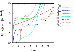
Figure 1: The plot of $[b_{L}(r)-r_{L}]/2$ as a function of $r$ for neutron-proton scattering via the NijmII potential in the ${}^{2S+1}L_{J}$ channel.

V.2 Coupled Channels

We now analyze channels with coupled partial waves.  We plot Eq. (71) and Eq. (72) for all coupled channels with $J\leq 3$.  The physical region correspond both $f_{J-1}(r)\geq 0$ and $g_{J+1}(r)\geq 0$.

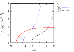
Figure 2: The plot of $f_{J-1}(r)$ as a function of $r$ for neutron-proton scattering via the NijmII potential for $J\leq 3$. Here $f_{1}(r)$ is rescaled by a factor of $0.01$ and $f_{2}(r)$ is rescaled by a factor of $10^{-4}$.

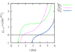
Figure 3: The plot of $g_{J+1}(r)$ as a function of $r$ for neutron-proton scattering via the NijmII potential for $J\leq 3$. Here $g_{3}(r)$ is rescaled by a factor of $0.1$.

V.2.1 $\,{}^{3}$S₁-$\,{}^{3}$D₁ Coupling.

We now consider Eq. (55) - (60) for the ${}^{3}S_{1}$-${}^{3}D_{1}$ coupled channel. We evaluate the Wronskians for $J=1$ and get

$$b_{0}(r)-q_{0}^{2}\frac{6}{r^{3}}-r_{0}=2\int_{0}^{r}\left(\left[U_{\alpha}^{(0)}(r^{\prime})\right]^{2}+\left[V_{\alpha}^{(0)}(r^{\prime})\right]^{2}\right)dr^{\prime},$$ (80)

$$b_{2}(r)+q_{0}^{2}\frac{2r^{3}}{3a_{2}^{2}}-r_{2}=2\int_{0}^{r}\left(\left[U_{\beta}^{(0)}(r^{\prime})\right]^{2}+\left[V_{\beta}^{(0)}(r^{\prime})\right]^{2}\right)dr^{\prime},$$ (81)

$$d_{1}(r)-q_{1}\frac{2}{a_{2}}=2\int_{0}^{r}[U_{0\alpha}(r^{\prime})U_{0\beta}(r^{\prime})+V_{0\alpha}(r^{\prime})V_{0\beta}(r^{\prime})]\,dr^{\prime}.$$ (82)

$b_{0}(r)$ and $b_{2}(r)$ are given in Eq. (75) and in Eq. (77), respectively, and $d_{1}(r)$ is

$$d_{1}(r)=-q_{0}\frac{1}{a_{0}a_{2}}\frac{2r^{3}}{3}+q_{0}\frac{1}{a_{2}}\frac{4r^{2}}{5}-q_{0}\frac{6}{r^{3}}.$$ (83)

Using the scattering parameters in Table 2 - 3, we plot Eq. (80), Eq. (81) and Eq. (82) as functions of $r$. In Fig. (4) we show the physical region where the causality bounds $f_{0}(r)\geq 0$, $g_{2}(r)\geq 0$, and $f_{0}(r)g_{2}(r)\geq h_{1}^{2}(r)$, are satisfied.  Here we have

$$f_{0}(r)=\frac{2}{3a_{0}^{2}}r^{3}-\frac{2}{a_{0}}r^{2}+2r-q_{0}^{2}\frac{6}{r^{3}}-r_{0},$$ (84)

$$g_{2}(r)=\frac{2}{1575a_{2}^{2}}r^{7}-\frac{2}{5a_{2}}r^{2}-\frac{6}{r^{3}}+q_{0}^{2}\frac{2r^{3}}{3a_{2}^{2}}-r_{2},$$ (85)

$$h_{1}(r)=-q_{0}\frac{1}{a_{0}a_{2}}\frac{2r^{3}}{3}+q_{0}\frac{1}{a_{2}}\frac{4r^{2}}{5}-q_{0}\frac{6}{r^{3}}-q_{1}\frac{2}{a_{2}}.$$ (86)

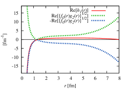
Figure 4: We plot Re$\left[\sqrt{f_{0}(r)g_{2}(r)}\right]$, $-$Re$\left[\sqrt{f_{0}(r)g_{2}(r)}\right]$, and Re$\left[h_{1}(r)\right]$ as functions of $r$ for neutron-proton scattering in ${}^{3}S_{1}$-${}^{3}D_{1}$ coupled channel.

V.2.2 $\,{}^{3}$P${}_{2}-\,^{3}$F₂ Coupling.

In the ${}^{3}P_{2}$-${}^{3}F_{2}$ coupled channel Eq. (55) - (60) take the following forms,

$$b_{1}(r)-q_{0}^{2}\frac{90}{r^{5}}-r_{1}=2\int_{0}^{r}\left(\left[U_{\alpha}^{(0)}(r^{\prime})\right]^{2}+\left[V_{\alpha}^{(0)}(r^{\prime})\right]^{2}\right)dr^{\prime},$$ (87)

$$b_{3}(r)+q_{0}^{2}\frac{1}{a_{3}^{2}}\frac{2r^{5}}{45}-r_{3}=2\int_{0}^{r}\left(\left[U_{\beta}^{(0)}(r^{\prime})\right]^{2}+\left[V_{\beta}^{(0)}(r^{\prime})\right]^{2}\right)dr^{\prime},$$ (88)

$$d_{2}(r)-q_{1}\frac{2}{a_{3}}=2\int_{0}^{r}[U_{0\alpha}(r^{\prime})U_{0\beta}(r^{\prime})+V_{0\alpha}(r^{\prime})V_{0\beta}(r^{\prime})]\,dr^{\prime}.$$ (89)

$b_{1}(r)$ and $b_{3}(r)$ are defined in Eq. (76) and Eq. (78), respectively, and $d_{2}(r)$ is

$$d_{2}(r)=-q_{0}\frac{1}{a_{1}a_{3}}\frac{2r^{5}}{45}+q_{0}\frac{1}{a_{3}}\frac{4r^{2}}{21}-q_{0}\frac{90}{r^{5}}.$$ (90)

The causality bounds are $f_{1}(r)\geq 0$, $g_{3}(r)\geq 0$, and $f_{1}(r)g_{3}(r)\geq h_{2}^{2}(r)$, where

$$f_{1}(r)=\frac{2r^{5}}{45a_{1}^{2}}-\frac{2r^{2}}{3a_{1}}-\frac{2}{r}-q_{0}^{2}\frac{90}{r^{5}}-r_{1},$$ (91)

$$g_{3}(r)=\frac{2r^{9}}{99225a_{3}^{2}}-\frac{2r^{2}}{7a_{3}}-\frac{90}{r^{5}}+q_{0}^{2}\frac{1}{a_{3}^{2}}\frac{2r^{5}}{45}-r_{3},$$ (92)

$$h_{2}(r)=-q_{0}\frac{1}{a_{1}a_{3}}\frac{2r^{5}}{45}+q_{0}\frac{1}{a_{3}}\frac{4r^{2}}{21}-q_{0}\frac{90}{r^{5}}-q_{1}\frac{2}{a_{3}}.$$ (93)

In Fig. (5) we show the physical region for the ${}^{3}P_{2}$-${}^{3}F_{2}$ coupled channel wave functions.

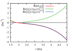
Figure 5: We plot Re$\left[\sqrt{f_{1}(r)g_{3}(r)}\right]$, $-$Re$\left[\sqrt{f_{1}(r)g_{3}(r)}\right]$, and Re$\left[h_{2}(r)\right]$ as functions of $r$ for neutron-proton scattering in ${}^{3}P_{2}$-${}^{3}F_{2}$ coupled channel. The functions are rescaled by a factor of $0.01$.

V.2.3 $\,{}^{3}$D${}_{3}-\,^{3}$G₃ Coupling.

For $J=3$, the ${}^{3}D_{3}$ and ${}^{3}G_{3}$ channels are coupled. In this case Eq. (55)-(60) read

$$b_{2}(r)-q_{0}^{2}\frac{3150}{r^{7}}-r_{2}=2\int_{0}^{r}\left(\left[U_{\alpha}^{(0)}(r^{\prime})\right]^{2}+\left[V_{\alpha}^{(0)}(r^{\prime})\right]^{2}\right)dr^{\prime},$$ (94)

$$b_{4}(r)+\frac{q_{0}^{2}}{a_{4}^{2}}\frac{2r^{7}}{1575}-r_{4}=2\int_{0}^{r}\left(\left[U_{\beta}^{(0)}(r^{\prime})\right]^{2}+\left[V_{\beta}^{(0)}(r^{\prime})\right]^{2}\right)dr^{\prime},$$ (95)

$$d_{3}(r)-q_{1}\frac{2}{a_{4}}=2\int_{0}^{r}[U_{0\alpha}(r^{\prime})U_{0\beta}(r^{\prime})+V_{0\alpha}(r^{\prime})V_{0\beta}(r^{\prime})]\,dr^{\prime}.$$ (96)

Here $d_{3}(r)$ is

$$d_{3}(r)=-\frac{q_{0}}{a_{2}a_{4}}\frac{2r^{7}}{1575}+q_{0}\frac{1}{a_{4}}\frac{4r^{2}}{45}-q_{0}\frac{3150}{r^{7}}.$$ (97)

The causality bounds are again $f_{2}(r)\geq 0$, $g_{4}(r)\geq 0$, and $f_{2}(r)g_{4}(r)\geq h_{3}^{2}(r)$, where

$$f_{2}(r)=\frac{2r^{7}}{1575a_{2}^{2}}-\frac{2r^{2}}{5a_{2}}-\frac{6}{r^{3}}-q_{0}^{2}\frac{3150}{r^{7}}-r_{2},$$ (98)

$$g_{4}(r)=\frac{2r^{11}}{9823275a_{4}^{2}}-\frac{2r^{2}}{9a_{4}}-\frac{3150}{r^{7}}+\frac{q_{0}^{2}}{a_{4}^{2}}\frac{2r^{7}}{1575}-r_{4},$$ (99)

$$h_{3}(r)=-\frac{q_{0}}{a_{2}a_{4}}\frac{2r^{7}}{1575}+q_{0}\frac{1}{a_{4}}\frac{4r^{2}}{45}-q_{0}\frac{3150}{r^{7}}-q_{1}\frac{2}{a_{4}}.$$ (100)

We show plots for the ${}^{3}D_{3}$-${}^{3}G_{3}$ channel in Fig. (6).

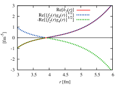
Figure 6: We plot Re$\left[\sqrt{f_{2}(r)g_{4}(r)}\right]$, $-$Re$\left[\sqrt{f_{2}(r)g_{4}(r)}\right]$, and Re$\left[h_{3}(r)\right]$ as functions of $r$ for neutron-proton scattering in ${}^{3}D_{3}$-${}^{3}G_{3}$ coupled channel. The functions are rescaled by a factor of $0.01$.

VI Results and Discussion

In this section we present the results for the causal and Cauchy-Schwarz ranges, $R^{b}$, and $R^{\text{C-S}}$.  We use the NijmII scattering data for neutron-proton scattering presented above.  In Table 4 we show results for the causal range for all uncoupled channels by setting

$$r_{L}=b_{L}(r).$$ (101)

In Table 5 we determine the causal range for all coupled channels using Eq. (71)-(72).  Also, we find the Cauchy-Schwarz ranges shown in Table 6 using Eq. (70).

Table 4: The causal ranges for uncoupled channels.

Channels	${}^{1}S_{0}$	${}^{1}P_{1}$	${}^{3}P_{0}$	${}^{3}P_{1}$	${}^{1}D_{2}$	${}^{3}D_{2}$	${}^{1}F_{3}$	${}^{3}F_{3}$
$R^{b}$ [fm]	$\ 1.27\$	$\ 0.31\$	$\ 3.07\$	$\ 0.23\$	$\ 3.98\$	$\ 4.91\$	$\ 1.88\$	$\ 1.56$

Table 5: The causal ranges for coupled channels.

Channels	${}^{3}S_{1}$	${}^{3}D_{1}$	${}^{3}P_{2}$	${}^{3}F_{2}$	${}^{3}D_{3}$	${}^{3}G_{3}$
$R^{b}$ [fm]	$\ 1.29\$	$\ 1.20\$	$\ 2.23\$	$\ 1.73\$	$\ 4.03\$	$\ 3.92$

Table 6: The Cauchy-Schwarz ranges for coupled channels.

Channels	${}^{3}S_{1}$-${}^{3}D_{1}$	${}^{3}P_{2}$-${}^{3}F_{2}$	${}^{3}D_{3}$-${}^{3}G_{3}$
$R^{\text{C-S}}$ [fm]	$\ 1.29\$	$\ 4.65\$	$\ 5.68\$

We find that in some channels the causal and Cauchy-Schwarz ranges are surprisingly large, and it is worthwhile to probe the origin of these large ranges.

It is convenient to collect together some of the key formulas derived above.  The Cauchy-Schwarz inequality has the form

$$f_{J-1}(r)g_{J+1}(r)\geq\left[h_{J}(r)\right]^{2},$$ (102)

where

$$f_{J-1}(r)=b_{J-1}(r)-2q_{0}^{2}\frac{\Gamma(J+\frac{1}{2})\Gamma(J+\frac{3}{2})}{\pi}\left(\frac{r}{2}\right)^{-2J-1}-r_{J-1},$$ (103)

$$g_{J+1}(r)=b_{J+1}(r)+\frac{2q_{0}^{2}}{a_{J+1}^{2}}\frac{\pi}{\Gamma(J+\frac{1}{2})\Gamma(J+\frac{3}{2})}\left(\frac{r}{2}\right)^{2J+1}-r_{J+1},$$ (104)

$$h_{J}(r)=d_{J}(r)-q_{1}\frac{2}{a_{J+1}},$$ (105)

$$b_{J\mp 1}(r) =\frac{1}{a_{J\mp 1}^{2}}\frac{2\pi}{\Gamma\left(J\mp 1+\frac{3}{2}\right)\Gamma\left(J\mp 1+\frac{5}{2}\right)}\left(\frac{r}{2}\right)^{2(J\mp 1)+3}$$

$$-\frac{1}{a_{J\mp 1}}\frac{4}{J\mp 1+\frac{1}{2}}\left(\frac{r}{2}\right)^{2}-\frac{2\Gamma\left(J\mp 1-\frac{1}{2}\right)\Gamma\left(J\mp 1+\frac{1}{2}\right)}{\pi}\left(\frac{r}{2}\right)^{-2(J\mp 1)+1},$$ (106)

$$d_{J}(r)= \frac{-q_{0}}{a_{J-1}a_{J+1}}\frac{2\pi}{\Gamma\left(\frac{1}{2}+J\right)\Gamma\left(\frac{3}{2}+J\right)}\left(\frac{r}{2}\right)^{2J+1}$$

$$+\frac{q_{0}}{a_{J+1}}\frac{4}{(2J-1)(2J+3)}r^{2}-2q_{0}\frac{\Gamma\left(J+\frac{1}{2}\right)\Gamma\left(J+\frac{3}{2}\right)}{\pi}\left(\frac{r}{2}\right)^{-2J-1}.$$ (107)

We note that the leading power of $r$ in $g_{J+1}(r)$ is

$$\frac{1}{a_{J+1}^{2}}\frac{2\pi}{\Gamma\left(J+1+\frac{3}{2}\right)\Gamma\left(J+1+\frac{5}{2}\right)}\left(\frac{r}{2}\right)^{2J+5}.$$ (108)

This has a very small numerical prefactor multiplying $a_{J+1}^{-2}r^{2J+5}$.  For $J=1$ the factor is $2/1575$, for $J=2$ it is $2/99225$, and for $J=3$ it is $2/9823275$.  Therefore the term is negligible unless $r$ is large compared with $(a_{J+1})^{1/(2J+3)}$.  If we neglect this term, then the term with the leading power of $r$ on the left hand side of Eq. (102) is the same as that on the right hand side,

$$\frac{1}{a_{J-1}^{2}}\frac{2\pi}{\Gamma\left(J-1+\frac{3}{2}\right)\Gamma\left(J-1+\frac{5}{2}\right)}\left(\frac{r}{2}\right)^{2J+1}\cdot\frac{2q_{0}^{2}}{a_{J+1}^{2}}\frac{\pi}{\Gamma(J+\frac{1}{2})\Gamma(J+\frac{3}{2})}\left(\frac{r}{2}\right)^{2J+1}$$

$$=\left[\frac{-q_{0}}{a_{J-1}a_{J+1}}\frac{2\pi}{\Gamma\left(\frac{1}{2}+J\right)\Gamma\left(\frac{3}{2}+J\right)}\left(\frac{r}{2}\right)^{2J+1}\right]^{2}.$$ (109)

As a result the curves for $f_{J-1}(r)g_{J+1}(r)$ and $\left[h_{J}(r)\right]^{2}$ are approximately parallel for large $r$ until the term that we have neglected becomes significant.  These nearly parallel trajectories inflate the value of the Cauchy-Schwarz range $r=R^{\text{C-S}}$ where the two curves cross.

For the ${}^{3}S_{1}$-${}^{3}D_{1}$ coupled channel we find $R^{\text{C-S}}$ is about the same size as the Compton wavelength of the pion, $m_{\pi}^{-1}=1.5$ fm.  This is also comparable to what one expects for the range of the nucleon-nucleon interaction.  However the results are more interesting for $J>1$.  In the ${}^{3}P_{2}$-${}^{3}F_{2}$ channel we have $R^{\text{C-S}}=4.65$ fm.  And for the ${}^{3}D_{3}$-${}^{3}G_{3}$ coupled channel we find $R^{\text{C-S}}$ $=$ $5.68$ fm.  These values are surprisingly large in comparison with $m_{\pi}^{-1}$.

VII One-Pion Exchange Potential

We note that there are some channels where the causal range $R^{b}$ is also quite large.  By definition $R^{\text{C-S}}\geq R^{b}$ and so the Cauchy-Schwarz range will then also be large.  The causal range is the minimum value for $r$ such that

$$f_{J-1}(r)=b_{J-1}(r)-2q_{0}^{2}\frac{\Gamma(J+\frac{1}{2})\Gamma(J+\frac{3}{2})}{\pi}\left(\frac{r}{2}\right)^{-2J-1}-r_{J-1}\geq 0$$ (110)

for the lower partial wave, or

$$g_{J+1}(r)=b_{J+1}(r)+\frac{2q_{0}^{2}}{a_{J+1}^{2}}\frac{\pi}{\Gamma(J+\frac{1}{2})\Gamma(J+\frac{3}{2})}\left(\frac{r}{2}\right)^{2J+1}-r_{J+1}\geq 0$$ (111)

for the higher partial wave.  For uncoupled channels we take $q_{0}=0$.

The largest values for $R^{b}$ occur when the effective range parameter is positive or near zero.  See for example the causal ranges for the ${}^{1}D_{2}$, ${}^{3}D_{2}$, ${}^{3}D_{3}$, and ${}^{3}G_{3}$ channels. What happens is that the function $f_{J-1}(r)$ or $g_{J+1}(r)$ remains negative with a rather small slope until $r$ becomes quite large.  The small slope is again associated with the fact that the term with the highest power of $r$ has a small numerical prefactor.

The range of the interaction plays the dominant role in setting the causal range.  In the language of local potentials, this is the radius at which the magnitude of the potential is numerically very small.  However there is also some influence of the exponential tail of the potential upon the causal range.

In all channels where the causal range is unusually large, ${}^{1}D_{2}$, ${}^{3}D_{2}$, ${}^{3}D_{3}$, and ${}^{3}G_{3}$, we find that the tail of the one-pion exchange potential is attractive.  At smaller radii, the potential crosses over at some classical turning point to become repulsive.  See for example Fig. 2-4 in Ref. Stoks et al. (1994).

The detailed mechanism requires further study, but it appears that this geometry can cause a near-threshold wavepacket to reflect before reaching the classical turning point, thus mimicking a longer range potential.  However some fine tuning is needed to produce a large causal range, as there is no enhancement in the ${}^{1}S_{0}$ and ${}^{3}S_{1}$ channels and a smaller amount of enhancement in the ${}^{3}P_{0}$ channel.

There seems to be no such enhancement of the causal range in the ${}^{1}P_{1}$, ${}^{3}P_{1}$, and ${}^{3}D_{1}$ channels where the tail of the potential is repulsive.  In fact, the causal range for the ${}^{1}P_{1}$ and ${}^{3}P_{1}$ channels are unusually small.  This appears be related to quantum tunneling into the inner region where the potential is attractive.

In the following analysis we will investigate the importance of the tail of the one-pion exchange potential plays in setting the causal range, $R^{b}$.  We show that even though the one-pion exchange potential is numerically small at distances larger than $5\,\text{fm}$, chopping off the one-pion exchange tail at such distances produces a non-negligible effect.  The one-pion exchange potential tail appears to be the source of the large values for $R^{b}$ in higher partial waves where the central one-pion exchange tail is attractive.

If we neglect electromagnetic effects, then the neutron-proton interaction potential at long distances is governed by the one-pion exchange (OPE) potential, which in configuration space is

$$V_{OPE}(r)=V_{C}(r)+S_{12}V_{T}(r).$$ (112)

Here $V_{C}(r)$ is the central potential,

$$V_{C}(r)=\frac{g_{\pi N}^{2}}{12\pi}\left(\frac{m_{\pi}}{2M_{N}}\right)^{2}(\vec{\tau}_{1}\cdot\vec{\tau}_{2})(\vec{\sigma}_{1}\cdot\vec{\sigma}_{2})\frac{e^{-m_{\pi}r}}{r},$$ (113)

$V_{T}(r)$ is the tensor potential,

$$V_{T}(r)=\frac{g_{\pi N}^{2}}{12\pi}\left(\frac{m_{\pi}}{2M_{N}}\right)^{2}\ (\vec{\tau}_{1}\cdot\vec{\tau}_{2})\ \Big{(}1+\frac{3}{m_{\pi}r}+\frac{3}{(m_{\pi}r)^{2}}\Big{)}\frac{e^{-m_{\pi}r}}{r},$$ (114)

and $S_{12}$ is the tensor operator,

$$S_{12}=3(\vec{\sigma_{1}}\cdot\hat{r})(\vec{\sigma_{2}}\cdot\hat{r})-\vec{\sigma_{1}}\cdot\vec{\sigma_{2}}.$$ (115)

Here $m_{\pi}$ is the pion mass, $M_{N}$ is the nucleon mass, and $g_{\pi N}=13.0$ is the pion-nucleon coupling constant.  The one-pion exchange potential is local in space and the interaction matrix in Eq. (14) takes the following form for $J=1$,

$$W(r,r^{\prime})=\left(\begin{array}[c]{cc}V_{C}(r)&\sqrt{8}V_{T}(r)\\ \sqrt{8}V_{T}(r)&V_{C}(r)-2V_{T}(r)\end{array}\right)\delta(r-r^{\prime}).$$ (116)

In Fig. (7) we plot $W_{11}(r)=V_{C}(r)$, $W_{12}(r)=W_{21}(r)=\sqrt{8}V_{T}(r),$ and $W_{22}(r)=V_{C}(r)-2V_{T}(r)$ in the ${}^{3}S_{1}$-${}^{3}D_{1}$ coupled channel.

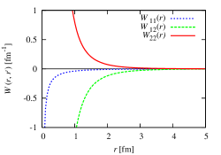
Figure 7: Plot of the potential matrix elements $W_{11}(r)=V_{C}(r)$, $W_{12}(r)=W_{21}(r)=\sqrt{8}V_{T}(r)$ and $W_{22}(r)=V_{C}(r)-2V_{T}(r)$ as a function of $r$ in the ${}^{3}S_{1}$-${}^{3}D_{1}$ coupled channel.

To demonstrate the origin of large causal ranges found in Table 4 and Table 5, we will present some simple but illustrative numerical examples.  For each channel we add a short range potential to the one-pion exchange potential in order to reproduce the physical low-energy scattering parameters. The specific model we use for the short range potential is not important to our general analysis nor is it the most economical.  We choose a simple scheme which consists of three well-defined functions in three different regions and which is continuously differentiable everywhere.  The potential has the form

$$V(r) =V_{\text{Gauss}}(r)\theta(R_{\text{Gauss}}-r)+V_{\text{Spline}}(r)\theta(r-R_{\text{Gauss}})\theta(R_{\text{Exch.}}-r)$$

$$+V_{\text{Exch.}}(r)\theta(r-R_{\text{Exch.}}),$$ (117)

where $\theta$ is a unit step function.

The short-range part is a Gaussian function

$$V_{\text{Gauss}}(r)=C_{G}e^{-m_{G}^{2}r^{2}}.$$ (118)

The intermediate-range part of the potential is a cubic spline use to connect the short- and long-range regions,

$$V_{\text{Spline}}(r)=C_{1}+C_{2}r+C_{3}r^{2}+C_{4}r^{3}.$$ (119)

The long-range part consists of the usual one-pion exchange potential together with two additional heavy meson exchange terms,

$$V_{\text{Exch.}}(r)=V_{C}^{\pi,A,B}(r)+S_{12}V_{T}^{\pi,D,F}(r).$$ (120)

The central part of the potential is composed of Yukawa functions

$$V_{C}^{\pi,A,B}(r)=\frac{g_{\pi N}^{2}}{12\pi}\left(\frac{m_{\pi}}{2M_{N}}\right)^{2}\left\{C_{\pi}\frac{e^{-m_{\pi}r}}{r}+C_{A}\frac{e^{-m_{A}r}}{r}+C_{B}\frac{e^{-m_{B}r}}{r}\right\},$$ (121)

and the tensor part of the potential has the form

$$V_{T}^{\pi,D,F}(r) =\frac{g_{\pi N}^{2}}{12\pi}\left(\frac{m_{\pi}}{2M_{N}}\right)^{2}\left\{C_{\Pi}\left[1+\frac{3}{m_{\pi}r}+\frac{3}{(m_{\pi}r)^{2}}\right]\frac{e^{-m_{\pi}r}}{r}\right.\hskip 156.49014pt$$

$$\left.+C_{D}\left[1+\frac{3}{m_{D}r}+\frac{3}{(m_{D}r)^{2}}\right]\frac{e^{-m_{D}r}}{r}+C_{F}\left[1+\frac{3}{m_{F}r}+\frac{3}{(m_{F}r)^{2}}\right]\frac{e^{-m_{F}r}}{r}\right\}.$$ (122)

Here $C_{\pi}=(2\vec{S}^{2}-3)(2\vec{T}^{2}-3)$, $C_{\Pi}=2\vec{T}^{2}-3$, $g_{\pi N}=13.0$, $m_{\pi}=140\,\text{MeV}$, and $M_{N}=938.0$ MeV. The coefficients not part of the one-pion exchange potential are used as free parameters to reproduce the physical low-energy scattering parameters.  Due to the abundance of free parameters, the fit process is not unique.  But in each case we attempt to qualitatively reproduce the shape of the NijmegenII potentials Stoks et al. (1994).  And in each case the heavy meson masses are kept significantly larger than the pion mass.  In Fig. (8) we show the potential in the ${}^{1}P_{1}$ channel.   Fig. (9) shows the potential in the ${}^{1}D_{2}$ channel, and Fig. (10) shows the potential in the ${}^{3}D_{2}$ channel.

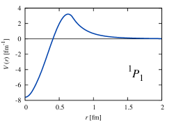
Figure 8: Plot of the model potential in the ${}^{1}P_{1}$ channel. In this channel $S=0$, $T=0$, $C_{\pi}=9$, $C_{A}=405.9$, $C_{B}=769.5$, $C_{\Pi}=0$, $C_{D}=0$, $C_{F}=0$, $C_{G}=-7.6$, $m_{A}=10.0m_{\pi}$, $m_{B}=5.45m_{\pi}$, $m_{G}=4.46m_{\pi}$, $C_{1}=-7.464$, $C_{2}=0.179$, $C_{3}=73.933$ and $C_{4}=-78.011$. We use $R_{\text{Gauss}}=0.2$ fm and $R_{\text{Exch.}}=0.7$ fm.

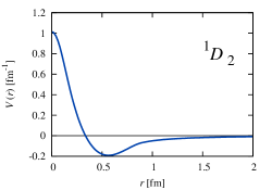
Figure 9: Plot of the model potential in the ${}^{1}D_{2}$ channel. In this channel $S=0$, $T=1$, $C_{\pi}=-3$, $C_{A}=-60.5$, $C_{B}=-30.0$, $C_{\Pi}=0$, $C_{D}=0$, $C_{F}=0$, $C_{G}=1.01$, $m_{A}=9m_{\pi}$, $m_{B}=6m_{\pi}$, $m_{G}=7.02m_{\pi}$, $C_{1}=1.463$, $C_{2}=-7.332$, $C_{3}=10.384$ and $C_{4}=-4.585$. We use $R_{\text{Gauss}}=0.2$ fm and $R_{\text{Exch.}}=0.9$ fm.

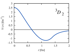
Figure 10: Plot of the model potential in the ${}^{3}D_{2}$ channel. In this channel $S=1$, $T=0$, $C_{\pi}=-3$, $C_{A}=-660$, $C_{B}=-1140$, $C_{\Pi}=-3$, $C_{D}=-930$, $C_{F}=-927$, $C_{G}=2.53$, $m_{A}=m_{D}=8m_{\pi}$, $m_{B}=m_{F}=5m_{\pi}$, $m_{G}=3.25m_{\pi}$, $C_{1}=2.979$, $C_{2}=-4.026$, $C_{3}=-2.455$ and $C_{4}=2.409$.  We use $R_{\text{Gauss}}=0.3$ fm and $R_{\text{Exch.}}=1.4$ fm.

After having recovered the physical low-energy scattering parameters, we now multiply an additional step function to the potential,

$$V(r)\rightarrow V(r)\theta(R-r),$$ (123)

which removes the tail of the potential beyond range $R$.  We then recalculate the low-energy scattering parameters with this modification.  The results are shown in Table 7 for the ${}^{1}P_{1}$, ${}^{1}D_{2}$, and ${}^{3}D_{2}$ channels.  The causal ranges for the ${}^{1}D_{2}$ and ${}^{3}D_{2}$ channels are quite large for the physical scattering data, $4.0$ and $4.9$ fm respectively.  But if we remove the tail of the model potential at $R=5$ fm, the causal ranges drop to $2.4$ and $2.7$ fm respectively.

Table 7: The potential range dependence of the causal range in various channels.

	$R=2\ \text{fm}$	$R=5\ \text{fm}$	$R=12\ \text{fm}$	$R=15\ \text{fm}$	$R=50\ \text{fm}$
$R_{{}^{1}P_{1}}^{b}$	0.4	0.4	0.3	0.3	0.3
$R_{{}^{1}D_{2}}^{b}$	2.0	2.4	3.8	4.0	4.0
$R_{{}^{3}D_{2}}^{b}$	1.3	2.7	4.7	4.9	4.9

The tail of the model potential is dominated by the one-pion exchange potential.  Even though the numerical size of the one-pion exchange potential is small at distances of $5$ fm, these numerical results show clearly that the one-pion exchange tail is controlling the size of the causal range.  The one-pion exchange potential tail appears to be the source of the large values for $R^{b}$ in higher partial waves where the central one-pion exchange tail is attractive.

VIII Summary and Conclusions

In this paper we have derived the constraints of causality and unitarity for neutron-proton scattering for all spin channels up to $J=3$.  We have defined and calculated interaction length scales which we call the causal range, $R^{b}$, and the Cauchy-Schwarz range, $R^{\text{C-S}}$.  The causal range is the minimum value for $r$ such that the causal bounds,

$$f_{J-1}(r)=b_{J-1}(r)-2q_{0}^{2}\frac{\Gamma(J+\frac{1}{2})\Gamma(J+\frac{3}{2})}{\pi}\left(\frac{r}{2}\right)^{-2J-1}-r_{J-1}\geq 0,$$ (124)

$$g_{J+1}(r)=b_{J+1}(r)+\frac{2q_{0}^{2}}{a_{J+1}^{2}}\frac{\pi}{\Gamma(J+\frac{1}{2})\Gamma(J+\frac{3}{2})}\left(\frac{r}{2}\right)^{2J+1}-r_{J+1}\geq 0,$$ (125)

are satisfied.  For uncoupled channels these bounds simplify to the form

$$f_{L}(r)=g_{L}(r)=b_{L}(r)\geq 0.$$ (126)

For coupled channels the Cauchy-Schwarz range is the minimum value for $r$ satisfying the causal bounds as well as the Cauchy-Schwarz inequality,

$$f_{J-1}(r)g_{J+1}(r)\geq\left[h_{J}(r)\right]^{2}.$$ (127)

If one reproduces the physical scattering data using strictly finite range interactions, then the range of these interactions must be larger than $R^{b}$ and $R^{\text{C-S}}$.  From these bounds we have derived the general result that non-vanishing partial-wave mixing cannot be reproduced with zero-range interactions.  As the range of the interaction goes to the zero, the effective range for the lower partial-wave channel is driven to negative infinity.

This finding has consequences for pionless effective theory where the range of the interactions is set entirely by the value of the cutoff momentum.  If the cutoff momentum is too high, then it is impossible to obtain the correct threshold physics in coupled channels without violating causality or unitarity.  In some channels we find that the causal range and Cauchy-Schwarz range are as large $5$ fm.  We have shown that these large values are driven by the tail of the one-pion exchange potential.  In these channels the problems will be even more severe, and the cutoff momentum will need to be rather low in order to reproduce the physical scattering data in pionless effective field theory.  How low this cutoff momentum must be depends on the particular regularization scheme.

We should note that all of these mixing observables are non-vanishing only when one reaches higher orders in the power counting expansion, and there is no direct impact on pionless effective field theory calculations at lower orders.  See, for example, Ref. Chen et al. (1999) for details on power counting in pionless effective field theory.  In the zero-range limit, the term which drives the negative divergence of the effective range parameter $r_{J-1}$ is

$$-2q_{0}^{2}\frac{\Gamma(J+\frac{1}{2})\Gamma(J+\frac{3}{2})}{\pi}\left(\frac{r}{2}\right)^{-2J-1}.$$ (128)

At leading order there is no divergence since there is no partial wave mixing and $q_{0}=0$.  If higher-order terms are iterated non-perturbatively as in Ref. van Kolck (1999b), then the divergence appears at order $Q^{2}$, the first order at which $q_{0}$ is non-vanishing.  If higher-order terms are iterated order-by-order in perturbation theory, then the term in Eq. (128) appears at order $Q^{4}$.  This is one order higher than the analysis presented in Ref. Chen et al. (1999), and we predict that zero-range divergences in $r_{J-1}$ will first appear at this order.

It important to note that if one works order-by-order in perturbation theory, then the constraints of causality and unitarity always appear somewhat hidden. At every order in the effective field theory calculation there are new operator coefficients which appear and are determined by matching to physical data. There are no obstructions to setting these operator coefficients to reproduce physical values.

It is only when one iterates the new interactions, i.e., by solving the Schrödinger equation, that non-linear dependencies on the operator coefficients appear. In this case one finds that the constraints of causality and unitarity give necessary conditions for keeping the operator coefficients real. Once we fix the regularization, the bound corresponds with branch cuts of the effective theory when viewed as a function of physical scattering parameters.

These branch cuts cannot be seen at any finite order in perturbation theory. However a nearby branch point may spoil the convergence of the perturbative expansion. In this context, our causality and unitarity bounds can be viewed as setting physical constraints for the convergence of perturbative calculations in pionless effective field theory.

If the cutoff is taken too high, a branch cut develops which jeopardizes the convergence of the perturbative calculation. Similarly if one does calculations using dimensional regularization, then the renormalization scale sets the scale at which the infrared and ultraviolet physics are regulated Georgi (1992). Similar problems with perturbative convergence would arise if the renormalization scale is taken too high.

There is much theoretical interest in the connection between dilute neutron matter and the universal physics of fermions in the unitarity limit Gezerlis and Carlson (2008); Borasoy et al. (2008); Epelbaum et al. (2009b); Lee (2008); Gezerlis and Carlson (2010); Wlazlowski and Magierski (2011); McNeil Forbes et al. (2012).  In the limit of isospin symmetry our analysis of the isospin triplet channels can be applied to neutron-neutron scattering in dilute neutron matter.  In this paper we have shown there are intrinsic length scales associated with the causal range and the Cauchy-Schwarz range.  When the average separation between neutrons is smaller than these length scales, one expects non-universal behavior controlled by the details of the neutron-neutron interactions. For the ${}^{1}S_{0}$ channel, $R^{b}=1.3$ fm.  For the ${}^{3}P_{2}$ channel, $R^{b}=2.2$ fm, and for the ${}^{3}F_{2}$ channel, $R^{b}=1.7$ fm.  For ${}^{3}P_{2}$-${}^{3}F_{2}$ mixing, we find $R^{\text{C-S}}=4.7$ fm.  We see that the physics of ${}^{3}P_{2}$-${}^{3}F_{2}$ mixing will become non-universal at lower densities than the ${}^{1}S_{0}$ interactions.  In particular the densities where ${}^{3}P_{2}$ superfluidity is expected to occur will be well beyond this universal regime.

Appendix A Functions

A.1 The Riccati-Bessel Functions

$S_{J\pm 1}(r)$ and $C_{J\pm 1}(r)$ are Riccati-Bessel functions of the first and second kind, which are defined in terms of the Bessel functions as

$$S_{J\pm 1}(r)=\sqrt{\frac{\pi r}{2}}J_{J\pm 1+\frac{1}{2}}(r)=\sqrt{\pi}r^{J\pm 1+1}\sum_{n=0}^{\infty}\frac{i^{2n}2^{-2n-J\mp 1-1}}{\Gamma(n+1)\Gamma(n+J\pm 1+\frac{3}{2})}r^{2n},$$ (129)

$$C_{J\pm 1}(r) =-\sqrt{\frac{\pi r}{2}}Y_{J\pm 1+\frac{1}{2}}(r)$$

$$=\frac{r^{-J\mp 1}}{\sqrt{\pi}}\Gamma(-J\mp 1+\frac{1}{2})\Gamma(J\pm 1+\frac{1}{2})\sum_{n=0}^{\infty}\frac{i^{2n}2^{-2n+J\pm 1}}{\Gamma(n+1)\Gamma(n-J\mp 1+1/2)}r^{2n}.$$ (130)

The $s(r)$ and $c(r)$ functions in Eq. (38) and Eq. (39) are written from Eq. (129) and Eq. (130),

$$s_{0,J\pm 1}(r) =\frac{\sqrt{\pi}}{\Gamma\left(J\pm 1+\frac{3}{2}\right)}\left(\frac{r}{2}\right)^{J\pm 1+1},$$ (131)

$$s_{2,J\pm 1}(r) =-\frac{\sqrt{\pi}}{\Gamma\left(J\pm 1+\frac{5}{2}\right)}\left(\frac{r}{2}\right)^{J\pm 1+3},$$ (132)

$$c_{0,J\pm 1}(r) =\frac{\Gamma\left(J\pm 1+\frac{1}{2}\right)}{\sqrt{\pi}}\left(\frac{r}{2}\right)^{-J\mp 1},$$ (133)

$$c_{2,J\pm 1}(r) =\frac{\Gamma\left(J\pm 1-\frac{1}{2}\right)}{\sqrt{\pi}}\left(\frac{r}{2}\right)^{-J\mp 1+2}.$$ (134)

A.2 Wronskians of Wave Functions

Here we calculate Wronskians of the $U(r)$ and $V(r)$ wave functions, and Wronskians of all possible combination of the $s_{0}(r)$, $s_{2}(r)$, $c_{0}(r)$ and $c_{2}(r)$ functions.  Wronskians of $U_{\alpha}(r)$ and $V_{\alpha}(r)$ for the non-interacting region $r\geq R$ are

$$W[U_{a\alpha}(r),U_{b\alpha}(r)] =(k_{a}^{2}-k_{b}^{2})\Big{\{}\frac{1}{2}r_{J-1}W[s_{0}(r),c_{0}(r)]_{J-1}$$

$$+\frac{1}{a_{J-1}^{2}}W[s_{2}(r),s_{0}(r)]_{J-1}+\frac{1}{a_{J-1}}W[c_{0}(r),s_{2}(r)]_{J-1}$$

$$+\frac{1}{a_{J-1}}W[s_{0}(r),c_{2}(r)]_{J-1}+W[c_{2}(r),c_{0}(r)]_{J-1}\Big{\}}$$

$$+\mathcal{O}(k_{a}^{4})+\mathcal{O}(k_{b}^{4}),$$ (135)

$$W[V_{a\alpha}(r),V_{b\alpha}(r)]=(k_{a}^{2}-k_{b}^{2})q^{2}W[c_{2}(r),c_{0}(r)]_{J+1}+\mathcal{O}(k_{a}^{4})+\mathcal{O}(k_{b}^{4}).$$ (136)

Wronskians of the $\beta$-state wave functions are

$$W[U_{a\beta}(r),U_{b\beta}(r)]=(k_{a}^{2}-k_{b}^{2})q^{2}\frac{1}{a_{J+1}^{2}}W[s_{2}(r),s_{0}(r)]_{J-1}+\mathcal{O}(k_{a}^{4})+\mathcal{O}(k_{b}^{4}),$$ (137)

$$W[V_{a\beta}(r),V_{b\beta}(r)] =(k_{a}^{2}-k_{b}^{2})\Big{\{}\frac{1}{2}r_{J+1}W[s_{0}(r),c_{0}(r)]_{J+1}$$

$$+\frac{1}{a_{J+1}^{2}}W[s_{2}(r),s_{0}(r)]_{J+1}+\frac{1}{a_{J+1}}W[c_{0}(r),s_{2}(r)]_{J+1}$$

$$+\frac{1}{a_{J+1}}W[s_{0}(r),c_{2}(r)]_{J+1}+W[c_{2}(r),c_{0}(r)]_{J+1}\Big{\}}$$

$$+\mathcal{O}(k_{a}^{4})+\mathcal{O}(k_{b}^{4}).$$ (138)

Wronskian of the combinations of the $\alpha$ and $\beta$-states are

$$W[U_{a\alpha}(r),U_{b\beta}(r)] =q\frac{1}{a_{J+1}}W[c_{0}(r),s_{0}(r)]_{J-1}-k_{a}^{2}\Big{\{}q\frac{1}{a_{J-1}a_{J+1}}W[s_{2}(r),s_{0}(r)]_{J-1}$$

$$-q\frac{1}{a_{J+1}}W[c_{2}(r),s_{0}(r)]_{J-1}\Big{\}}+k_{b}^{2}\Big{\{}q\frac{1}{a_{J-1}a_{J+1}}W[s_{2}(r),s_{0}(r)]_{J-1}$$

$$-q\frac{1}{a_{J+1}}W[s_{2}(r),c_{0}(r)]_{J-1}+q\frac{r_{J+1}}{2}W[s_{0}(r),c_{0}(r)]_{J-1}$$

$$-q_{1}\frac{1}{a_{J+1}}W[s_{0}(r),c_{0}(r)]_{J-1}\Big{\}}+\mathcal{O}(k^{4}),\hskip 128.0374pt$$ (139)

$$W[U_{a\beta}(r),U_{b\alpha}(r)] =-q\frac{1}{a_{J+1}}W[c_{0}(r),s_{0}(r)]_{J-1}+k_{b}^{2}\Big{\{}q\frac{1}{a_{J-1}a_{J+1}}W[s_{2}(r),s_{0}(r)]_{J-1}$$

$$-q\frac{1}{a_{J+1}}W[c_{2}(r),s_{0}(r)]_{J-1}\Big{\}}-k_{a}^{2}\Big{\{}q\frac{1}{a_{J-1}a_{J+1}}W[s_{2}(r),s_{0}(r)]_{J-1}$$

$$-q\frac{1}{a_{J+1}}W[s_{2}(r),c_{0}(r)]_{J-1}+q\frac{r_{J+1}}{2}W[s_{0}(r),c_{0}(r)]_{J-1}$$

$$-q_{1}\frac{1}{a_{J+1}}W[s_{0}(r),c_{0}(r)]_{J-1}\Big{\}}+\mathcal{O}(k^{4}),\hskip 128.0374pt$$ (140)

$$W[V_{a\alpha}(r),V_{b\beta}(r)] =-q\frac{1}{a_{J+1}}W[c_{0}(r),s_{0}(r)]_{J+1}-{k_{a}^{2}}\Big{\{}q_{1}\frac{1}{a_{J+1}}W[c_{0}(r),s_{0}(r)]_{J+1}$$

$$+q\frac{1}{a_{J+1}}W[c_{2}(r),s_{0}(r)]_{J+1}-qW[c_{2}(r),c_{0}(r)]_{J+1}\Big{\}}$$

$$+{k_{b}^{2}}\Big{\{}q\frac{r_{J+1}}{2}W[c_{0}(r),s_{0}(r)]_{J+1}-q\frac{1}{a_{J+1}}W[c_{0}(r),s_{2}(r)]_{J+1}$$

$$+qW[c_{0}(r),c_{2}(r)]_{J+1}\Big{\}}+\mathcal{O}(k^{4}),$$ (141)

$$W[V_{a\beta}(r),V_{b\alpha}(r)] =q\frac{1}{a_{J+1}}W[c_{0}(r),s_{0}(r)]_{J+1}+{k_{b}^{2}}\Big{\{}q_{1}\frac{1}{a_{J+1}}W[c_{0}(r),s_{0}(r)]_{J+1}$$

$$+q\frac{1}{a_{J+1}}W[c_{2}(r),s_{0}(r)]_{J+1}-qW[c_{2}(r),c_{0}(r)]_{J+1}\Big{\}}$$

$$-{k_{a}^{2}}\Big{\{}q\frac{r_{J+1}}{2}W[c_{0}(r),s_{0}(r)]_{J+1}-q\frac{1}{a_{J+1}}W[c_{0}(r),s_{2}(r)]_{J+1}$$

$$+qW[c_{0}(r),c_{2}(r)]_{J+1}\Big{\}}+\mathcal{O}(k^{4}).$$ (142)

We now calculate Wronskians of the $s_{0}(r)$, $s_{2}(r)$, $c_{0}(r)$ and $c_{2}(r)$ functions.  We find

$$W[s_{0}(r),s_{2}(r)]_{J}=-\frac{\pi}{\Gamma\left(\frac{3}{2}+J\right)\Gamma\left(\frac{5}{2}+J\right)}\left(\frac{r}{2}\right)^{3+2J},$$ (143)

$$W[s_{0}(r),c_{0}(r)]_{J}=-1,$$ (144)

$$W[s_{0}(r),c_{2}(r)]_{J}=-\frac{r^{2}}{2+4J},$$ (145)

$$W[s_{2}(r),c_{0}(r)]_{J}=\frac{r^{2}}{2+4J},$$ (146)

$$W[s_{2}(r),c_{2}(r)]_{J}=\frac{r^{4}}{16J(J+1)-12},$$ (147)

$$W[c_{0}(r),c_{2}(r)]_{J}=-\frac{\Gamma\left(-\frac{1}{2}+J\right)\Gamma\left(\frac{1}{2}+J\right)}{\pi}\left(\frac{r}{2}\right)^{1-2J}.$$ (148)

It should be noted that $W[f(r),g(r)]=-W[f(r),g(r)]$.

Appendix B Relations between Eigenphase and Nuclear Bar Parameterizations

The scattering matrix in terms of the eigenphase parameters was given in Eq. (24).  The scattering matrix in terms of the nuclear bar parameters is

$$S=\left(\begin{array}[c]{cc}e^{2i\bar{\delta}_{\alpha}}\cos 2\bar{\varepsilon}&ie^{i\left(\bar{\delta}_{\alpha}+\bar{\delta}_{\beta}\right)}\sin 2\bar{\varepsilon}\\ ie^{i\left(\bar{\delta}_{\alpha}+\bar{\delta}_{\beta}\right)}\sin 2\bar{\varepsilon}&e^{2i\bar{\delta}_{\beta}}\cos 2\bar{\varepsilon}\end{array}\right).$$ (149)

Here $\overline{\delta}_{\alpha}$, $\overline{\delta}_{\beta}$ and $\overline{\varepsilon}$ are the nuclear bar phase shifts and mixing angle Stapp et al. (1957).  The relations between the eigenphase and the nuclear bar parameters are

$$\sin(\delta_{\alpha}-\delta_{\beta}) =\frac{\sin 2\overline{\varepsilon}}{\sin 2{\varepsilon}},$$ (150)

$$\delta_{\alpha}+\delta_{\beta} =\overline{\delta}_{\alpha}+\overline{\delta}_{\beta},$$ (151)

$$\tan 2\varepsilon =\frac{\tan 2\overline{\varepsilon}}{\sin(\overline{\delta}_{\alpha}-\overline{\delta}_{\beta})}.$$ (152)

The two-channel effective range expansion is defined slightly differently in the eigenphase and the nuclear bar parameterizations.  In the eigenphase parameterization,

$$k^{L_{ij}+\frac{1}{2}}U\hat{\mathbf{K}}^{-1}U^{-1}k^{L_{ij}+\frac{1}{2}}=-\frac{1}{a_{ij}}+\frac{1}{2}r_{ij}k^{2}+\mathcal{O}(k^{4}),$$ (153)

and in the nuclear bar parameterization,

$$k^{L_{ij}+\frac{1}{2}}\hat{\mathbf{K}}^{-1}k^{L_{ij}+\frac{1}{2}}=-\frac{1}{\bar{a}_{ij}}+\frac{1}{2}\bar{r}_{ij}k^{2}+\mathcal{O}(k^{4}).$$ (154)

Therefore, by straightforward calculations we find the following relations among the threshold scattering parameters,

$$a_{\alpha}= \bar{a}_{\alpha},$$ (155)

$$r_{\alpha}= \bar{r}_{\alpha}+\frac{2\bar{q}_{0}\bar{q}_{1}}{\bar{a}_{\alpha}}+\frac{\bar{q}^{2}\bar{r}_{\beta}}{\bar{a}_{\alpha}^{2}},$$ (156)

$$a_{\beta}= \bar{a}_{\beta}-\frac{\bar{q}_{0}^{2}}{\bar{a}_{\alpha}},$$ (157)

$$r_{\beta}= \bar{r}_{\beta},$$ (158)

$$q_{0}= \frac{\bar{q}_{0}}{\bar{a}_{\alpha}},$$ (159)

$$q_{1}= \frac{\left(\bar{a}_{\beta}\bar{a}_{\alpha}-\bar{q}_{0}^{2}\right)\left(\bar{a}_{\alpha}\bar{q}_{1}+\bar{r}_{\beta}\bar{q}_{0}\right)}{2\bar{a}_{\alpha}^{2}}.$$ (160)

For the uncoupled channels $q_{0}$ and $q_{1}$ are zero, and these relations become $a_{\alpha}=\bar{a}_{\alpha}$, $r_{\alpha}=\bar{r}_{\alpha}$, $a_{\beta}=\bar{a}_{\beta}$, and $r_{\beta}=\bar{r}_{\beta}$.

References

- van Kolck (1999a) U. van Kolck, Prog. Part. Nucl. Phys. 43, 337 (1999a), eprint nucl-th/9902015.
- Bedaque and van Kolck (2002) P. F. Bedaque and U. van Kolck, Ann. Rev. Nucl. Part. Sci. 52, 339 (2002), eprint nucl-th/0203055.
- Epelbaum (2006) E. Epelbaum, Prog. Part. Nucl. Phys. 57, 654 (2006), eprint nucl-th/0509032.
- Epelbaum et al. (2009a) E. Epelbaum, H.-W. Hammer, and U.-G. Meißner, Rev. Mod. Phys. 81, 1773 (2009a), eprint arXiv:0811.1338 [nucl-th].
- van Kolck (1999b) U. van Kolck, Nucl. Phys. A645, 273 (1999b), eprint nucl-th/9808007.
- Bedaque et al. (1999a) P. F. Bedaque, H.-W. Hammer, and U. van Kolck, Phys. Rev. Lett. 82, 463 (1999a), eprint nucl-th/9809025.
- Bedaque et al. (1999b) P. F. Bedaque, H.-W. Hammer, and U. van Kolck, Nucl. Phys. A646, 444 (1999b), eprint nucl-th/9811046.
- Bedaque et al. (2000) P. F. Bedaque, H.-W. Hammer, and U. van Kolck, Nucl. Phys. A676, 357 (2000), eprint nucl-th/9906032.
- Chen et al. (1999) J.-W. Chen, G. Rupak, and M. J. Savage, Nucl. Phys. A653, 386 (1999), eprint nucl-th/9902056.
- Platter et al. (2005) L. Platter, H.-W. Hammer, and U.-G. Meißner, Phys. Lett. B607, 254 (2005), eprint nucl-th/0409040.
- Hammer and Platter (2007) H. W. Hammer and L. Platter, Eur. Phys. J. A32, 113 (2007), eprint nucl-th/0610105.
- Braaten and Hammer (2006) E. Braaten and H.-W. Hammer, Phys. Rept. 428, 259 (2006).
- Giorgini et al. (2008) S. Giorgini, L. P. Pitaevskii, and S. Stringari, Rev. Mod. Phys. 80, 1215 (2008), eprint arXiv:0706.3360v2 [cond-mat.other].
- Wigner (1955) E. P. Wigner, Phys. Rev. 98, 145 (1955).
- Phillips and Cohen (1997) D. R. Phillips and T. D. Cohen, Phys. Lett. B390, 7 (1997), eprint nucl-th/9607048.
- Pavon Valderrama and Arriola (2006) M. Pavon Valderrama and E. R. Arriola, Phys. Rev. C74, 054001 (2006), eprint nucl-th/0506047.
- Calle Cordon and Ruiz Arriola (2010) A. Calle Cordon and E. Ruiz Arriola, Phys. Rev. C81, 044002 (2010), eprint 0905.4933.
- Calle Cordón and Ruiz Arriola (2010) A. Calle Cordón and E. Ruiz Arriola, Phys. Rev. A 81, 044701 (2010).
- Hammer and Lee (2009) H. W. Hammer and D. Lee, Phys. Lett. B681, 500 (2009), eprint arXiv:0907.1763 [nucl-th].
- Hammer and Lee (2010) H. W. Hammer and D. Lee, Annals Phys. 325, 2212 (2010), eprint arXiv:1002.4603 [nucl-th].
- Blatt and Biedenharn (1952) J. M. Blatt and L. C. Biedenharn, Phys. Rev. 86, 399 (1952).
- Lee (2009) D. Lee, Prog. Part. Nucl. Phys. 63, 117 (2009), eprint arXiv:0804.3501 [nucl-th].
- Koehler et al. (2006) T. Koehler, K. Goral, and P. S. Julienne, Rev. Mod. Phys. 78, 1311 (2006), eprint cond-mat/0601420.
- Regal and Jin (2006) C. Regal and D. S. Jin (2006), eprint cond-mat/0601054.
- Stapp et al. (1957) H. P. Stapp, T. J. Ypsilantis, and N. Metropolis, Phys. Rev. 105, 302 (1957).
- Biedenharn and Blatt (1954) L. C. Biedenharn and J. M. Blatt, Phys. Rev. 93, 1387 (1954).
- Elhatisari and Lee (2012) S. Elhatisari and D. Lee (2012), eprint arXiv:1206.1207v1.
- Stoks et al. (1993) V. G. J. Stoks, R. A. M. Klomp, M. C. M. Rentmeester, and J. J. de Swart, Phys. Rev. C 48, 792 (1993).
- Valderrama and Arriola (2005) M. P. Valderrama and E. R. Arriola, Phys. Rev. C 72, 044007 (2005).
- Stoks et al. (1994) V. G. J. Stoks, R. A. M. Klomp, C. P. F. Terheggen, and J. J. de Swart, Phys. Rev. C 49, 2950 (1994).
- Georgi (1992) H. Georgi, Nucl. Phys. Proc. Suppl. 29BC, 1 (1992).
- Gezerlis and Carlson (2008) A. Gezerlis and J. Carlson, Phys. Rev. C77, 032801 (2008), eprint 0711.3006.
- Borasoy et al. (2008) B. Borasoy, E. Epelbaum, H. Krebs, D. Lee, and U.-G. Meißner, Eur. Phys. J. A35, 357 (2008), eprint 0712.2993.
- Epelbaum et al. (2009b) E. Epelbaum, H. Krebs, D. Lee, and U.-G. Meißner, Eur. Phys. J. A40, 199 (2009b), eprint 0812.3653.
- Lee (2008) D. Lee, Phys. Rev. C78, 024001 (2008), eprint 0803.1280.
- Gezerlis and Carlson (2010) A. Gezerlis and J. Carlson, Phys. Rev. C81, 025803 (2010), eprint 0911.3907.
- Wlazlowski and Magierski (2011) G. Wlazlowski and P. Magierski, Phys. Rev. C83, 012801 (2011), eprint 0912.0373.
- McNeil Forbes et al. (2012) M. McNeil Forbes, S. Gandolfi, and A. Gezerlis (2012), eprint 1205.4815.