Activity of comet 103P/Hartley 2 at the time of the EPOXI mission fly-by††thanks: Based on Observations performed at the European Southern Observatory, La Silla, Progr. 086.C-0375. This work has been partially funded by MIUR - Ministero dell’Istruzione, dell’universitá e della Ricerca, under the PRIN 2008 funding.
Abstract
Comet 103P/Hartley 2 was observed on Nov. 1-6, 2010, coinciding with the fly-by of the space probe EPOXI. The goal was to connect the large scale phenomena observed from the ground, with those at small scale observed from the spacecraft. The comet showed strong activity correlated with the rotation of its nucleus, also observed by the spacecraft. We report here the characterization of the solid component produced by this activity, via observations of the emission in two spectral regions where only grain scattering of the solar radiation is present. We show that the grains produced by this activity had a lifetime of the order of 5 hours, compatible with the spacecraft observations of the large icy chunks. Moreover, the grains produced by one of the active regions have a very red color. This suggests an organic component mixed with the ice in the grains.
keywords:
Comets , Comets, dust , Comets, coma1 Introduction
Comet 103P/Hartley 2 (hereafter 103P) was discovered in March 1986 by M. Hartley, (1986) with the UK Schmidt Telescope at Siding Spring (Australia). Its dynamical history (Carusi et al.,, 1985, and following electronic updates) shows that its orbit has been quite unstable over the last 150 years, with a perihelion distance oscillating between 1 and 2.5 AU. 103P is one of the few comets that have become an Earth crosser in the recent past.
103P has been frequently observed over the 20 years following its discovery, both by ground-based and space telescopes. The portrait that emerged from this harvest of ground-based data (e.g. Licandro et al.,, 2000; Lowry & Fitzsimmons,, 2001; Lowry et al.,, 2003; Snodgrass et al.,, 2006, 2008; Mazzotta Epifani et al.,, 2008) is that of a highly active comet, even at large heliocentric distance (5 AU, Snodgrass et al.,, 2008). In October 2007, 103P was selected as the target for the NASA Deep Impact extended mission EPOXI (A’Hearn et al.,, 2005); consequently, an intense world-wide observation campaign has been devoted to characterize its nucleus and coma properties in order to prepare for the spacecraft fly-by, occurring in November 2010.
The main results of this campaign are summarized in Meech et al., (2011): the comet has a small, sub-km, nucleus, with a rotation period of 16.4 hrs when inactive, slowly increasing with activity. This possibly indicates that the rotation rate is slowed by out-gassing from the (irregular) surface.
The campaign data also showed that the active fraction of the nucleus’ surface is, as typical, about 2%, but that it is surrounded by a large halo of (icy?) grains that contribute more than the nucleus to the total water production rate ( 90% at perihelion). The presence of large grains was already inferred during the 1998 perihelion passage: analysis and modeling of ISOCAM (Cesarski et al.,, 1996) infrared images of the dust coma and tail (Epifani et al.,, 2001) implied an evolution of the dust production rate from 10 kg s-1 at 3.25 AU to 100 kg s-1 at 1.04 AU, with grains up to centimeters in size. This dust environment of 103P seems consistent with a trail structure (Lisse et al.,, 2009), presumably associated with millimeter-sized debris.
On UT 4.583 November 2010, the NASA mission spacecraft EPOXI flew by 103P. The closest approach was 694 km, when the comet was at 1.064 AU from the Sun. The main results of the in-situ measurements are described in A’Hearn et al., (2011): the nucleus showed a bi-lobed morphology, with a maximum length of 2.33 km and a mean radius of km. The rotation period at the time of the closest approach was measured to be h. Images obtained during the fly-by confirmed the presence of individual, “large” chunks near the nucleus, moving at 1–2 m s-1. Large grains had already been detected via radar observations just before the close encounter (Harmon et al.,, 2011): decimeter-sized grains (or possibly even larger), moving at 20–30 m s-1, and ejected into free trajectories rather than circum-nuclear orbits were modeled to fit the grain-coma echo from 103P. A’Hearn et al., (2011) argued that the largest chunks they detected from EPOXI were icy, with radii up to 10–20 cm, dragged out by super-volatiles (specifically, CO2) and then sublimating to provide a large fraction of the total H2O gaseous output of the comet.
Here we report observations done during 5 (half) nights around the time of the space probe fly-by. The observations were obtained with narrow band filters centered in regions with continuum emission, i.e. due to the scattering of solar radiation by the grains present in the coma.
2 Observations and data reduction
All the observations were performed with EFOSC111http://www.eso.org/sci/facilities/lasilla/instruments/efosc/ at the ESO 3.56 m New Technology Telescope (NTT), in La Silla (Chile). The observation epoch, geometry and conditions are listed in Table 1.
| Date | UTstr | rh | Phase | PA | Sky | Filt. | Texp | airm | |
|---|---|---|---|---|---|---|---|---|---|
| 2010 Nov. | hh:mm | AU | AU | s | |||||
| 01 | 07:59 | 1.06 | 0.143 | 58.4 | 280.4 | Pht | 560 | 1.43 | |
| ” | 08:18 | ” | ” | ” | ” | ” | 560 | 1.36 | |
| ” | 08:25 | ” | ” | ” | ” | ” | 5120 | 1.34 | |
| ” | 08:57 | ” | ” | ” | ” | ” | 7120 | 1.30 | |
| 03 | 08:10 | 01:06 | 0.151 | 58.7 | 282.6 | Pht | 5180 | 1.30 | |
| ” | 08:54 | ” | ” | ” | ” | ” | 5180 | 1.27 | |
| 04 | 07:43 | 1.06 | 0.154 | 58.8 | 283.7 | Clr | 5180 | 1.31 | |
| ” | 08:04 | ” | ” | ” | ” | ” | 5180 | 1.27 | |
| ” | 08:48 | ” | ” | ” | ” | ” | 5180 | 1.24 | |
| 05 | 05:10 | 1.06 | 0.156 | 58.8 | 284.6 | Pht | 8120 | 2.30 | |
| ” | 05:34 | ” | ” | ” | ” | ” | 8120 | 1.97 | |
| ” | 05:58 | ” | ” | ” | ” | ” | 8120 | 1.74 | |
| ” | 06:45 | ” | ” | ” | ” | ” | 8120 | 1.46 | |
| ” | 07:08 | ” | ” | ” | ” | ” | 8120 | 1.37 | |
| ” | 07:56 | ” | ” | ” | ” | ” | 8120 | 1.26 | |
| ” | 08:19 | ” | ” | ” | ” | ” | 8120 | 1.23 | |
| ” | 08:46 | ” | ” | ” | ” | ” | 8120 | 1.21 | |
| 06 | 05:03 | 1.06 | 0.163 | 58.8 | 285.6 | Pht | 8120 | 2.32 | |
| ” | 05:27 | ” | ” | ” | ” | ” | 8120 | 1.97 | |
| ” | 05:50 | ” | ” | ” | ” | ” | 8120 | 1.75 | |
| ” | 06:38 | ” | ” | ” | ” | ” | 8120 | 1.46 | |
| ” | 07:01 | ” | ” | ” | ” | ” | 8120 | 1.36 | |
| ” | 07:48 | ” | ” | ” | ” | ” | 8120 | 1.25 | |
| ” | 08:12 | ” | ” | ” | ” | ” | 8120 | 1.21 |
UTstr refers to the beginning of the observations; and are the helio- and geocentric distances; Phase is the Sun-Target-Observer angle; PA is the position angle of the extended Sun-Target vector. The sky conditions are listed: Pht is for photometric, Clr is for clear. Filt. is the identifier of the filter; Texp the is the sequence exposure time on target, in second; the airmass (airm) is listed for the beginning of each observations
Most of the observations consisted in images of the comet obtained through Narrow Band (NB) cometary filters (similar to those described in Farnham et al.,, 2000). The NB filters included blue and red continuum ( and ), (0-0) Violet band, and the Swan () bands. In this paper we focus on the solid component of the coma, i.e. the data obtained with the two continuum filters. Table 2 lists their central wavelengths and full widths at half maximum.
To minimize the contamination by background stars and to evaluate the sky background, each comet observation sequence consisted of 5 or 8 exposures on target, moving the telescope by few tens of arcseconds in between, and one additional exposure obtained 8′ off the comet, to record the sky uncontaminated by the comet.
Bias and twilight sky flat-field exposures were also obtained in order to correct for the instrumental signature. Spectrophotometric standard stars and solar analog stars were observed spectroscopically and also in imaging mode, with the same filters at about the same airmass as the comet, to calibrate in flux the comet images.
At the beginning of the run, some images of the comet were acquired through the standard broad band filters , and . They were not used in this analysis, because their pass-bands contain non negligible gas emission lines. This was verified a posteriori with the spectra.
| Filter Name | Central | FWHM |
|---|---|---|
| [Å] | [Å] | |
| 4430 | 33 | |
| 6840 | 74 |
All the images and spectra were at first corrected for bias and flat-field, using the appropriate ancillary frames in the customary manner. To calibrate the images in (see below) we computed the “theoretical” filter color indexes (-V and -V) of the observed spectrophotometric standard and solar analog stars. By using the tabulated spectra, we compared stellar fluxes measured through the NB and V filters to that of a star of A0V spectral type that, by definition, has a color index equal to 0. The knowledge of the V magnitude of the observed stars allowed us to recover the NB magnitudes and hence, from the observations, the photometric zero point (ZP) of each NB filter for each night.
For the extinction correction, we adopted the standard extinction of La Silla222 http://www.ls.eso.org/sci/facilities/lasilla/astclim/atm_ext/. Since the standard stars were observed at about the same airmass as at least one of the comet sequences, the errors introduced by possible differences in the extinctions are negligible. When more than one sequence with the same filter was observed, the resulting calibrated images were in agreement within 10%. The same agreement was found also for calibrated images from consecutive photometric nights, in regions of the coma where the signature produced by periodic change of activity (see below) was not yet present. All the frames with the same filter were then inter-calibrated (see below).
The level of the sky contribution was then evaluated for each comet sequence, measuring the median level of the sky frame acquired through the same filter away from the comet. This value was subtracted from each frame.
The sky-subtracted frames then were re-centered on the comet photometric center, and a composite comet image was obtained through a median average of the 5 or 8 frames of the sequence.
The use of a median combination significantly reduces the contamination produced by background stars. The background was then refined and subtracted with a trial and error procedure using the function (see below), by making this function independent of the projected nucleo-centric distance () for distances greater than 150 pixels (corresponding to 15000 km at the comet distance) from the photometric center. The resulting continuum images were then calibrated in (A’Hearn et al.,, 1984).
3 Analysis
3.1 1D analysis: background activity
As shown by the spacecraft observations (A’Hearn et al.,, 2011) and as already noticed at the telescope during the observations, the comet showed a strong variability with nucleus rotation. By studying the CN features in the coma, Samarasinha et al., (2011) found that rotation period varied from 17.1 h in September to 18.8 h in November 2010. Thus for this study we assume a rotation period of 18.8 h. We arbitrarily use as a starting point for the rotation phase the time of the first observation (not used here because it was recorded with a broad band filter). This point was Nov. 1, UT = 7:39.
To check how the emission of the continuum varied with the rotation period, we first characterized the constant background coma, which was estimated from the epoch of minimal activity.
A’Hearn et al., (1984) introduced the function as a proxy for production of the solid component. is the geometric albedo of the grains and the filling factor, defined as the percentage of the area that is covered by the grains, and the projected nucleo-centric distance of the aperture. Typically, the filling factor, , is proportional to , while is, at first approximation, independent of . Since from the observations we get the product , it is not possible to disentangle these two parameters without additional observations in the thermal IR or without making assumptions.
Here we used another function derived by the above one, i.e. (), that is proportional to the average column density of the solid component at the projected nucleo-centric distance . It is equal to . As shown by Tozzi et al., (2007), should be constant with respect to the projected nuclear distance, , for a comet with a dust outflow of constant velocity and production rate, and if sublimation or fragmentation of the grains are excluded. The solar radiation pressure introduces a small linear dependence with , but normally its effects are only noticeable at large distances from the nucleus, larger than the field of view (FoV) of EFOSC.
a.
b.
The final calibrated images were analyzed by computing their () function. In Fig. 1 some examples of the function are shown. The solid component production rate was clearly not constant, as it can be noticed by comparing the regions with 500-1000 km. However, excluding the region with smaller than about 3000–5000 km, the profiles are very similar, and the signatures of the change of activity seems to overlap that of a typical, constant profile.
Plotting all the profiles together, as shown in Fig. 1, we can see that they have the same behavior for greater that 3000-5000 km and the values of in that region are within . These differences are comparable to the uncertainty of the absolute calibration. We therefore assumed that the average value of over in the 6000–8000 km range was constant over the observations, and made small corrections to the Zero Points to adjust the profiles so they have the same average value over that range. This assumption is equivalent to considering that any change in grains production did not reach km from one day to the next. The validity of this hypothesis will be verified later. Note that using this method, the data acquired during the non-photometric night (Nov. 4) have been also calibrated to the same system as the others.
All the profiles are very similar except in the region very close to the nucleus ( 2000 km) where the signature of the activity seems confined. In order to characterize the periodic emissions, a profile corresponding to the minimum of cometary activity –what we call the “quiet comet”– was determined for each filter as follows: for the regions with 6000 km as a median of all the profiles, and for that with 6000 km as the minimum envelope of all the profiles (excluding the region with km). The median was used to reduce signatures of possible background stars, still present in the single profiles; the minimum envelope allowed us to discard the peaks produced by the activity. However, the always present activity in the regions with 100-200 km (see below) was visually removed by spline interpolation. The profiles, corresponding to the constant level of activity, are shown in Fig. 2 for both filters.

From the measurements of , the values of for in the 6000–8000 km range corresponded to 803 cm and 913 cm in and , respectively. The errors were obtained from the standard deviation of the values of the function, with the re-normalization described above.
From the above values of , it is possible to derive the slope of the reflectivity spectrum for the solid component coma of the “quiet comet”. Assuming a linear variation with lambda, the at =5550 Å would be 853 cm and the corresponding spectral slope would be 5.21.5 %/1000 Å.
As seen in Fig. 2, the profiles of the minimum activity are not completely constant with , but they systematically increase in the inner region of the coma up to equal to 2000–2500 km. Note that this behavior cannot be due to a residual background, because this would produce a linear variation with . A profile like that means that the total grain cross-section increases with in a systematic way. The only possible explanation is the fragmentation of large grains, with dimensions much larger than the observation wavelength, as they move away from the nucleus. In that way, the total grain cross-sections would increase with . It is important to notice that the behavior of the quiet coma can be found in all the profiles, even though, it is partially hidden by the periodic activity
3.2 Periodic activity
By subtracting the minimum profile for or from the individual profiles, we found the signature of the clouds of grains periodically ejected by the nucleus. Typical profiles of the those clouds are shown in Figure 3. All profiles are similar, with a very strong increase towards the nucleus. There is no evidence of any motion of the clouds, as it has been seen for other outbursts (see for instance Tozzi and Licandro,, 2002).

It would be interesting to determine the colors of the clouds of grains produced by the periodic activity, and to compare them to that of the coma at minimum activity. This measurement is complicated by the rapid evolution of the cloud and by the fact that the observations in and are taken at different times. To measure the color of the material produced by the activity, we have first to characterize its evolution with time.
We determined then the time when the comet was closer to the minimum activity, by checking the individual profiles and then selecting the minimum ones. They were those recorded on November 6 at UT 5:10 and 5:58 for the and filters, respectively. Their profiles are very similar to the minimum profiles derived above: only a narrow and faint peak is present in the region with 100-200 km, indicating that the periodic activity was starting again. By chance those two observations are very close to the rotation phase equal to 0 as defined in the previous section.
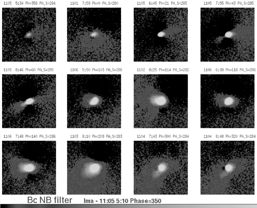
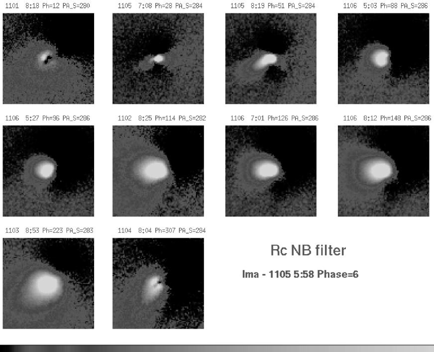
To map the emission produced by the periodic activity, we subtract these images corresponding to the minimum of activity from the individual images.
As pointed out above, those two images were not acquired at the exact minimum of activity: the inner part already shows the signs of the periodic activity emission. Nevertheless, these signs are limited to the very inner coma ( 200 km) and it is easy to take them into account in the following analysis.
The activity maps are shown as a function of the rotation phase in Figures 4 and 5 for the and filters, respectively. For clarity, the figures cover a limited FoV, equivalent to a projected area of 2000 2000 km2 centered on the comet. The FoV actually covered by the observations is more than 10 times larger. The grains released by the periodic activity are clearly visible in both filters. They are particularly evident in two preferred directions. The first one points to the East at position angle PA90and is active from a rotation phase of about 90 to 200. The second one points to PA 140and is active from the rotation phase greater than 200. They don’t seem produced by the same active region on the rotating nucleus, because in such a case we should see the produced grains spiraling around the nucleus.
We have then analyzed the two directions independently, to check whether the active regions have different origins, as found by the spacecraft (A’Hearn et al.,, 2011). The maps have been transformed to polar coordinates, and the profiles of the emission with respect to the nucleo-centric distance have been obtained by integrating between PA = 40 and 117 for the first cloud, and between PA = 118 to 165 for the second one. The profiles have been transformed in equivalent units (accounting for the limited angular range, as the standard definition of implies an integration over 2). Typical equivalent profiles of the cloud during a phase of high activity are shown in Fig. 6.
The profiles for the active regions are very similar to those presented earlier for the 1D analysis –only the peak intensity and signal-to-noise ratio (SNR) are different. Excluding the region with 200 km, which is dominated by the seeing of the image and contaminated by the near-nucleus activity in the reference image of the “quiet” comet, the profiles are very well represented by a constant plus an exponential function,
where is the scale length of the cloud released by the activity (in km), and the peak intensity (in cm). The fit residuals are very small, with errors less than 10% even for profiles with medium/high activity, i.e. with high SNR.
The variation of with time gives the projected expansion velocity of the grains located at . Of course grains located at have larger projected velocities and those at smaller distances have smaller velocities. Since the direction of the emission of the cloud of particles in space is not known, the projected velocities are a lower limit of the real expansion velocities. To get the projected velocity we used the observations from November 6, that are most numerous and that were obtained when the level of activity was relatively high. The resulting is –20 m s-1 for both clouds, which is comparable to the velocity of the grains measured by radar (Harmon et al.,, 2011). Note that they measured radial velocities, while we measured projected velocities.
Those low projected velocities imply that the cloud of grains produced by periodic activity cannot move to distances greater than about 1700 km in 24 hours. This implies the grains must still be well within the FoV for observations recorded during the following night. The assumption we had made before, that the grains had not reached a projected distance larger than 6000 km from one night to the next, is therefore valid, justifying our inter-normalization of the outer part of the profiles.
The equivalent functions are always peaked at close to 0, as can be seen in Fig. 3. A motion of the cloud away from the nucleus was never detected (apart the small increase of mentioned above) contrary to other comets, e.g. C/1999 S4 before its breakup (Tozzi and Licandro,, 2002) or 9P/Tempel 1 after the impact (Tozzi et al.,, 2007), for which a similar analysis revealed a clear motion of the ejecta with a Maxwellian profile.
The product gives the cross-sections, , of the released clouds, i.e. the total surface () covered by the grains multiplied by their geometric albedo ().

The values of together with those of the scale-length are reported in Table 3 for both filters. as function of the rotation phase is shown in Fig. 7.
| Date | UT | Rot. | PA80 | PA140 | ||
|---|---|---|---|---|---|---|
| 2010 Nov. | Phase | |||||
| [h:mm] | [] | [km] | [km2] | [km] | [km | |
| filter | ||||||
| 01 | 7:59 | 6 | 38526 | 0.03070.0026 | 27451 | 0.04270.0198 |
| 02 | 8:25 | 114 | 45214 | 0.13270.0050 | 10014 | 0.02930.0112 |
| 03 | 8:10 | 209 | 48711 | 0.13500.0036 | 127230 | 0.17770.0047 |
| 04 | 7:43 | 300 | 64229 | 0.05200.0026 | 142240 | 0.19090.0061 |
| 04 | 8:48 | 320 | 19722 | 0.04110.0100 | 194688 | 0.19750.0094 |
| 05 | 5:34 | 358 | - | - | - | - |
| 05 | 6:45 | 21 | - | - | - | - |
| 05 | 7:55 | 43 | - | - | - | - |
| 05 | 8:46 | 59 | - | - | 28113 | 0.04640.0038 |
| 06 | 5:50 | 103 | 277 5 | 0.06020.0013 | - | - |
| 06 | 6:38 | 118 | 26411 | 0.05330.0027 | - | - |
| 06 | 7:48 | 140 | 424 5 | 0.14220.0021 | 2166 | 0.04350.0020 |
| filter | ||||||
| 01 | 8:18 | 12 | 3166 | 0.05240.0015 | 98337 | 0.06420.0030 |
| 02 | 8:25 | 114 | 3674 | 0.20420.0032 | 3186 | 0.09290.0023 |
| 03 | 8:53 | 223 | 3564 | 0.16410.0020 | 164828 | 0.35290.0060 |
| 04 | 8:04 | 307 | 1934 | 0.06970.0016 | 155548 | 0.20230.0066 |
| 05 | 7:08 | 28 | 1086 | 0.01780.0019 | 1039 | 0.01490.0030 |
| 05 | 8:19 | 51 | 1481 | 0.07560.0011 | 2303 | 0.05630.0014 |
| 06 | 5:03 | 88 | 1861 | 0.09200.0011 | 1264 | 0.04060.0033 |
| 06 | 5:27 | 96 | 1841 | 0.09780.0013 | 994 | 0.04520.0053 |
| 06 | 7:01 | 126 | 2461 | 0.18370.0009 | 1814 | 0.05350.0023 |
| 06 | 8:12 | 148 | 3481 | 0.21300.0010 | 2743 | 0.08450.0015 |
a.
b.
3.2.1 PA 90
For the activity cloud released at PA90 the variations of for and filters with the phase have similar behaviors, with the values for lower than those of . By interpolating the points obtained with different phases, we see that, multiplying the intensities by 1.36, the two profiles overlap. As long as the grains are bigger than the wavelength, this is simply the variation of the albedo from to , i.e. the color of the grains. Note that in such a way those measurements of color are independent from any temporal change due to the variability of the emission. The error in the color of the grains has been evaluated as the standard deviation of the data with respect to an interpolating curve. It results of the order of 0.026 km2.
The albedo of the grains in is then 36% higher than in . Assuming a linear dependence with wavelength, the albedo at Å is 20% higher than that at and the spectral slope is (14.71.1) %/1000 Å. This value is more than 3 times larger than that of the background dust emission of the “quiet comet” obtained in the previous section.
In Fig. 7 (a), the derived from the observations with the filters have been multiplied by 1.36 to take into account the different albedos, in order to check how the cross-sections change with the rotation phase. The points from consecutive nights interleave nicely, suggesting the repeatability of the emission period after period. However, we cannot firmly prove this asserting. In fact, for example, the data at phase around 200 come from observations of Nov. 3 at UT 8-9, while the data for phase of 300 come from observations taken the day after, more or less at the same UT (see tables 3). That means that the nucleus had rotated by one full turn plus 100.
Assuming a typical grain albedo of , the maximum area covered by them is of the order of 5 km2. The variations of illustrated in Fig. 7 are very large: it varies from almost 0.04 km2, at phase close to 0, to more than 0.2 km2 at phase –200, with an increase of at least a factor of 5. The increases of between phase 0 to 200 can be simply explained with an increase of the production in the grains as the active area moves into sunlight.
Instead the factor of four decrease passing from phase 200 to phase 300(see Fig. 7, a), corresponding to about 5 h if the periodicity can be trusted (or 24 h actual elapsed time), is more difficult to explain: the cloud must still be well within the FoV of the observations because of the low projected velocity. This strongly supports the hypothesis that grains sublimated away, with a lifetime surely shorter than 24 h and probably of the order of 5 h. If they are transformed into gas, they will contribute no longer to the observations in the continuum bands.
The color of the grains ejected at this PA is similar to that of the surface of short period comets, Centaurs and scattered disk TNOs (see online MBOSS color database Hainaut & Delsanti,, 2002). This color cannot be explained by pure ice; they could be ice particles with a large amount of organic material or just organic grains that sublimate under the solar radiation.
3.2.2 PA 140
The clouds of particles released at PA 140 are much fainter and the data therefore are more noisy than the other ones. However the data taken through the filter overlap with those through the filter, within the errors. The estimated error is here about 0.05 km2. The corresponding spectral slope is then 02.4 %/1000 Å.
This cloud appears during a short range of rotation period, at a phase 200. The changes by a factor 6–7 during the whole rotation. As for the other cloud, it decreases by a factor 4 passing from rotation phase of 300to (360+)20, suggesting sublimating grains for this cloud as well.
However, these grains seem to have a gray color, in contrast to those released at PA90. The appearance of the two clouds at different rotation phases indicates that they are produced by different active regions of the nucleus, and the great difference in their color, suggest that these regions produce different kind of grains. Those at PA140 are more similar to the icy chunks discovered by the spacecraft, because ice should have gray color. Also those grains cannot be pure ices, since their lifetimes should be much longer that the 5 hours indicated here (see for example Beer et al., (2006)). So also these grains should have some impurities of gray color, as for example silicates.
4 Conclusions
From the analysis of images recorded in the blue and red continuum regions of the visible spectra, we have separated the solid state emission produced by the periodic activity from the normal dust cometary coma of the “quiet” comet.
We have found that the coma of the “quiet” comet shows a peculiar behavior: its function is not constant, but shows an increase with nucleo-centric distances , for 2000-2500 km, that is not typical of a comet with constant outflow velocity and without fragmentation or sublimation. The profiles of the “quiet coma” obtained over the 5 nights of observations have a very similar behavior. Of course this is true for the observations where the emission due to the periodic activity does not hide completely the inner coma. This kind of profile is an indication that the scattering of the grains increases as they move away from the nucleus. Since this behavior is the same during a long period of time (5 nights), the only explanation is that the grains present in the coma of the “quiet” comet fragment with the time, increasing their scattering area with the nucleo-centric distance.
The color of the solid state coma of the “quiet” comet is red, with a spectral slope of 4.61.5 %/1000 Å, assuming a linear variation with wavelength.
By analyzing the grains produced by the periodic activity we have shown that the released clouds have two privileged projected directions: one at PA90 and the other at 140. The profiles of the equivalent function with of the clouds released in the two direction can be fitted with a constant plus an exponential function. The cross-sections of the two clouds vary strongly with the rotation phase of the nucleus. They move very slowly, with projected velocities of the order of 20 m/s, for both PAs. One of the two clouds (the one with PA90) has a very red color, of the order of 153 %/1000 Å, while the other seems to have a gray color. Assuming a periodic emission with the rotation, both sublimate with lifetimes of the order of 5 h.
During the flyby, the spacecraft has observed for the first time some large chunks around the nucleus, that are supposed to be icy ice particles. The gray cloud can be then constituted by those chunks. However, to explain their relatively short lifetimes, those particles also need to have some impurities, gray in color, as for example silicates. The clouds released in the other direction are very red and sublimate as well with a lifetime of the order of few hours. So these grains should have lot of organics embedded in them, or they are pure organic grains that sublimate. It is important to notice that, within equal to 4000 km, i.e. where most of the activity takes place, the cross section of the clouds produced by the activity is at most 6% of that of the quiet comet. This is of the same order of magnitude of the 4% contribution of the icy chunks measured by the spacecraft (A’Hearn et al.,, 2011).
Once the full geometrical analysis of the jets observed by the spacecraft becomes available, it will be interesting to connect them with the two clouds described here, and to investigate whether their different characteristics can be traced to different natures of the sublimating area.
5 Acknowledgments
Based on Observations performed at the European Southern Observatory, La Silla, Progr. 086.C-0375. This work has been partially funded by MIUR - Ministero dell’Istruzione, dell’Universitá e della Ricerca (Italy), under the PRIN 2008 funding.
6 References
References
- A’Hearn et al., (1984) A’Hearn, M.F., Schleicher, D.G., Feldman, P.D, Millis R.L., & Thompson, D.T. 1984. Comet Bowell 1980b.0 AJ, 89, 579-591
- A’Hearn et al., (2005) A’Hearn M.F., Belton M.J.S., Delamere W.A. et al., 2005. Deep Impact: Excavating Comet Tempel 1. Science 310, 258-264
- A’Hearn et al., (2011) A’Hearn M.F., Belton M.J.S., Delamere W.A. et al., 2011. EPOXI at comet Hartley 2. Science 332, 1396-1400
- Beer et al., (2006) Beer, E. H., Podolack, M. Prialnik, D., 2006. The contribution of icy grains to the activity of comets I. Grain lifetime and distribution, Icarus, 180, 473-486
- Carusi et al., (1985) Carusi A., Kresak L., Perozzi E., Valsecchi G.B., 1985. Long-term Evolution of Short-period Comets. Text book, Adam Hilger, Bristol
- Cesarski et al., (1996) Cesarsky C.J. and 65 colleagues, 1996. ISOCAM in flight. A&A 315, L32-L37
- Epifani et al., (2001) Epifani E., Colangeli L., Fulle M., Brucato J.R., Bussoletti E., De Sanctis M.C., Mennella V., Palomba E., Palumbo P., Rotundi A., 2001. ISOCAM imaging of comets 103P/Hartley 2 and 2P/Encke. Icarus 149, 339-350
- Farnham et al., (2000) Farnham, T. L. and Schleicher, D. G. and A’Hearn, M. F., 2000.The HB Narrowband Comet Filters: Standard Stars and Calibrations. Icarus, 147, 180-204
- Hainaut & Delsanti, (2002) Hainaut, O.R. and Delsanti, A.C., 2002. Colors of Minor Bodies in the Outer Solar System - a Statistical Analysis. A&A 389, 641-664
- Harmon et al., (2011) Harmon J.K., Nolan M.C., Howell E.S., Giorgini J.D., Taylor P.A., 2011. Radar observations of comet 103P/Hartley 2. ApJ 734, L2-L4
- Hartley, (1986) Hartley M., 1986. Comet Hartley (1986c). IAU Circ. 4197
- Licandro et al., (2000) Licandro J., Tancredi G., Lindgren M., Rickman H., Hutton R. G., 2000. CCD Photometry of Cometary Nuclei, I: Observations from 1990-1995. Icarus 147, 161-179
- Lisse et al., (2009) Lisse C.M., Fernadez Y.R., Reach W.T., Bauer J.M., A’Hearn M.F., Farnham T.L., Groussin O., Belton M.J., Meech K.J., Snodgrass C.D., 2009. Spizer Space Telescope Observations of the Nucleus of Comet 103P/Hartley 2. PASP 121, 968-975
- Lowry & Fitzsimmons, (2001) Lowry S.C. & Fitzsimmons A., 2001.CCD photometry of distant comets. II. A&A 365, 204-213
- Lowry et al., (2003) Lowry S.C., Fitzsimmons A., Collander-Brown S., 2003. CCD photometry of distant comets. III – Ensemble properties of Jupiter-family comets. A&A 397, 329-343
- Mazzotta Epifani et al., (2008) Mazzotta Epifani E., Palumbo P., Capria M.T., Cremonese G., Fulle M., Colangeli L., 2008. The distant activity of Short Period Comets. II. MNRAS 390, 265-280
- Meech et al., (2011) Meech K.J., A’Hearn M.F., Adams J.A. et al., 2011. EPOXI: comet 103P/Hartley 2 observations from a worldwide campaign. ApJ 734, L1-l9
- Samarasinha et al., (2011) Samarasinha N.H., Mueller B.E.A., A’Hearn M.F., Farnham T.L., Gersch, A. 2011. Rotation of Comet Hartley2 from Structures in the Coma. ApJ letters, 734, L3-L6
- Snodgrass et al., (2006) Snodgrass C., Lowry S.C., Fitzsimmons A., 2006. Photometry of cometary nuclei: Rotation rates, colors and a comparison with Kuiper Belt Objects. MNRAS 373, 1590-1602
- Snodgrass et al., (2008) Snodgrass C., Lowry S.C., Fitzsimmons A., 2008. Optical observations of 23 distant Jupiter Family Comets, including 36P/Whipple at multiple phase angles. MNRAS 385, 737-756
- Tozzi and Licandro, (2002) Tozzi, G. P., and Licandro, J., 2002, Icarus. Visible and Infrared Images of C/1999 S4 (LINEAR) during the Disruption of Its Nucleus. 157, 187-192
- Tozzi et al., (2007) Tozzi, G. P., Boehnhardt, H., Kolokolova, L., et al., 2007, A&A. Dust observations of Comet 9P/Tempel 1 at the time of the Deep Impact. 476, 979-988