Estimates for approximation numbers of some classes of composition operators on the Hardy space

Abstract. We give estimates for the approximation numbers of composition operators on $H^{2}$, in terms of some modulus of continuity. For symbols whose image is contained in a polygon, we get that these approximation numbers are dominated by ${\rm e}^{-c\sqrt{n}}$. When the symbol is continuous on the closed unit disk and has a domain touching the boundary non-tangentially at a finite number of points, with a good behavior at the boundary around those points, we can improve this upper estimate. A lower estimate is given when this symbol has a good radial behavior at some point. As an application we get that, for the cusp map, the approximation numbers are equivalent, up to constants, to ${\rm e}^{-c\,n/\log n}$, very near to the minimal value ${\rm e}^{-c\,n}$. We also see the limitations of our methods. To finish, we improve a result of O. El-Fallah, K. Kellay, M. Shabankhah and H. Youssfi, in showing that for every compact set $K$ of the unit circle $\mathbb{T}$ with Lebesgue measure $0$, there exists a compact composition operator $C_{\varphi}\colon H^{2}\to H^{2}$, which is in all Schatten classes, and such that $\varphi=1$ on $K$ and $|\varphi|<1$ outside $K$.

Mathematics Subject Classification 2010. Primary: 47B06 – Secondary: 30J10 ; 47B33

Key-words. approximation numbers; Blaschke product; composition operator; cusp map; Hardy space; modulus of continuity; Schatten classes

1 Introduction and notation

If the approximation numbers of some classes of operators on Hilbert spaces are well understood (for example, those of Hankel operators: see [16]), it is not the case of those of composition operators. Though their behavior remains mysterious, some recent results are obtained in [14] and [12] for approximation numbers of composition operators on the Hardy space $H^{2}$. In [14], it is proved that one always has $a_{n}(C_{\varphi})\gtrsim{\rm e}^{-c\,n}$ for some $c>0$ ([14], Theorem 3.1) and that this speed of decay can only be got when the symbol $\varphi$ maps the unit disk $\mathbb{D}$ into a disk centered at $0$ of radius strictly less than $1$, i.e. $\|\varphi\|_{\infty}<1$ ([14], Theorem 3.4).

In this paper, we give estimates which are somewhat general, in terms of some modulus of continuity. In Section 2, we obtain an upper estimate when the symbol $\varphi$ is continuous on the closed unit disk and has an image touching non-tangentially the unit circle at a finite number of points, with a good behavior on the boundary around this point. As an application, we show that for symbols $\varphi$ whose image is contained in a polygon $a_{n}(C_{\varphi})\leq a\,{\rm e}^{-b\sqrt{n}}$, for some constants $a,b>0$; this has to be compared with [12], Proposition 2.7, where it is shown that if $\varphi$ is a univalent symbol such that $\varphi(\mathbb{D})$ contains an angular sector centered on the unit circle and with opening $\theta\pi$, $0<\theta<1$, then $a_{n}(C_{\varphi})\geq a\,{\rm e}^{-b\sqrt{n}}$, for some (other) positive constants $a$ and $b$, depending only on $\theta$. In Section 3, we obtain a lower bound when $\varphi$ has a good radial behavior at the contact point. Both proofs use Blaschke products. This allows to recover the estimation $a_{n}(C_{\lambda_{\theta}})\approx{\rm e}^{-c\,\sqrt{n}}$ obtained in [14], Proposition 6.3, and [12], Theorem 2.1 for the lens map $\lambda_{\theta}$. In Section 4.1, we give another example, the cusp map, for which $a_{n}(C_{\varphi})\approx{\rm e}^{-c\,n/\log n}$, very near the minimum value ${\rm e}^{-c\,n}$. We end that section by considering a one-parameter class of symbols, first studied by J. Shapiro and P. D. Taylor [22] and seeing the limitations of our methods. In Section 5, we improve a result of E.A. Gallardo-Gutiérrez and M.J. González (previously generalized by O. El-Fallah, K. Kellay, M. Shabankhah and H. Youssfi [5], Theorem 3.1). It is known that for every compact composition operator $C_{\varphi}\colon H^{2}\to H^{2}$, the set $E_{\varphi}=\{{\rm e}^{i\theta}\,;\ |\varphi^{\ast}({\rm e}^{i\theta})|=1\}$ has Lebesgue measure $0$. These authors showed ([6]), with a rather difficult construction, that there exists a compact composition operator $C_{\varphi}\colon H^{2}\to H^{2}$ such that the Hausdorff dimension of $E_{\varphi}$ is equal to $1$ (and in [5], it is shown that for any negligible compact set $K$, there is a Hilbert-Schmidt operator $C_{\varphi}$ such that $E_{\varphi}=K$). We improve this result in showing that for every compact set $K$ of the unit circle $\mathbb{T}$ with Lebesgue measure $0$, there exists a compact composition operator $C_{\varphi}\colon H^{2}\to H^{2}$, which is even in all Schatten classes, and such that $E_{\varphi}=K$.

Notation. We denote by $\mathbb{D}$ the open unit disk and by $\mathbb{T}=\partial\mathbb{D}$ the unit circle; $m$ is the normalized Lebesgue measure on $\mathbb{T}$: $dm(t)=dt/2\pi$. The disk algebra $A(\mathbb{D})$ is the space of functions which are continuous on the closed unit disk $\overline{\mathbb{D}}$ and analytic in the open unit disk. If $H^{2}$ is the usual Hardy space on $\mathbb{D}$, every analytic self-map $\varphi\colon\mathbb{D}\to\mathbb{D}$ (also called Schur function) defines, by Littlewood’s subordination principle, a bounded operator $C_{\varphi}\colon H^{2}\to H^{2}$ by $C_{\varphi}(f)=f\circ\varphi$, called the composition operator of symbol $\varphi$.

Recall that if $T\colon E\to F$ is a bounded operator between two Banach spaces, the approximation numbers $a_{n}(T)$ of $T$ are defined by:

$$\qquad\quad a_{n}(T)=\inf\{\|T-R\|\,;\ {\rm rank}\,(R)<n\}\,,\qquad n=1,2,\ldots$$

The sequence $\big{(}a_{n}(T)\big{)}_{n}$ is non-increasing and, when $F$ has the Approximation Property, $T$ is compact if and only if $a_{n}(T)$ tends to $0$.

Definition 1.1

A modulus of continuity $\omega$ is a continuous function

$$\omega\colon[0,A]\to\mathbb{R}^{+},$$

which is increasing, sub-additive, and vanishes at zero.

Some examples are:

$$\omega(h)=h^{\alpha},\quad 0<\alpha\leq 1\,;\qquad\omega(h)=h\log\frac{1}{h}\,;\qquad\omega(h)=\frac{1}{\log\frac{1}{h}}\,\cdot$$

For any modulus of continuity $\omega$, there is a concave modulus of continuity $\omega^{\prime}$ such that $\omega\leq\omega^{\prime}\leq 2\omega$ (see [17] for example); therefore we may and shall assume that $\omega$ is concave on $[0,A]$. In that case, $\omega^{-1}$ is convex, and

(1.1) $$r_{\omega}(x):=\frac{\omega^{-1}(x)}{x}$$

is non-decreasing.

The notation $u(t)\lesssim v(t)$ means that $u(t)\leq Av(t)$ for some constant $A>0$ and $u(t)\approx v(t)$ means that both $u(t)\lesssim v(t)$ and $v(t)\lesssim u(t)$.

2 Upper bound and boundary behavior

Definition 2.1

Let $\omega$ be a modulus of continuity and $\varphi$ a symbol in the disk algebra $A(\mathbb{D})$. Let $\xi_{0}\in\partial\mathbb{D}\cap\varphi(\overline{\mathbb{D}})$. We say that the symbol $\varphi$ has an $\omega$-regular behavior at $\xi_{0}$ if, setting:

(2.1) $$\gamma(t)=\varphi({\rm e}^{it})\,,$$

and $E_{\xi_{0}}=\{t\,;\ \gamma(t)=\xi_{0}\}$, there exists $r_{0}>0$ such that:

1) for some positive constant $C>0$, one has, for every $t_{0}\in E_{\xi_{0}}$ and $|t-t_{0}|\leq r_{0}$:

(2.2) $$|\gamma(t)-\gamma(t_{0})|\leq C\big{(}1-|\gamma(t)|\big{)}\,.$$

2) for some positive constant $c>0$, one has, for for every $t_{0}\in E_{\xi_{0}}$ and $|t-t_{0}|\leq r_{0}$:

(2.3) $$c\,\omega(|t-t_{0}|)\leq|\gamma(t)-\gamma(t_{0})|\,.$$

The first condition implies that the image of $\varphi$ touches $\partial\mathbb{D}$ at the point $\xi_{0}$, and non-tangentially. The second one implies that $\varphi$ does not stay long near $\xi_{0}=\gamma(t_{0})$.

Note that, due to (2.3), the intervals $[t-r_{0}/2,t+r_{0}/2]$, for $t\in E_{\xi_{0}}$ are pairwise disjoint and therefore the set $E_{\xi_{0}}$ must be finite.

We shall make the following assumption (to avoid the Lipschitz class):

(2.4) $$\qquad\lim_{h\to 0^{+}}\frac{\omega(h)}{h}=\infty\,;\quad\text{equivalently}\quad\lim_{h\to 0^{+}}\frac{\omega^{-1}(h)}{h}=0.$$

Indeed, assume that $\gamma$ is $K$-Lipschitz at some point $t_{0}\in[0,2\pi]$, namely $|\varphi({\rm e}^{it})-\varphi({\rm e}^{it_{0}})|\leq K\,|t-t_{0}|$, with $|\varphi({\rm e}^{it_{0}})|=1$; then

$$m(\{t\in[0,2\pi]\,;\,|\varphi({\rm e}^{it}) -\varphi({\rm e}^{it_{0}})|\leq h\})$$

$$\geq m(\{t\in[0,2\pi]\,;\,|t-t_{0}|\leq h/K\})=h/2\pi K\,;$$

hence this measure in not $o\,(h)$ and the composition operator $C_{\varphi}$ is not compact ([15], or [3], Theorem 3.12).

In order to treat the case where the image of $\varphi$ is a polygon, we need to generalize the above definition. We ask not only that $\varphi$ is $\omega$-regular at the points $\xi_{1},\ldots,\xi_{p}$ of contact of $\varphi(\overline{\mathbb{D}})$ with $\partial\mathbb{D}$, but a little bit more.

Definition 2.2

Assume that $\varphi(\overline{\mathbb{D}})\cap\partial\mathbb{D}=\{\xi_{1},\ldots,\xi_{p}\}$. We say that $\varphi$ is globally-regular if there exists a modulus of continuity $\omega$ such that, writing $E_{\xi_{j}}=\{t\,;\ \gamma(t)=\xi_{j}\}$, one has, for some $r_{1},\ldots,r_{p}>0$

$$\mathbb{T}=\bigcup_{j=1}^{p}\big{(}E_{\xi_{j}}+[-r_{j},r_{j}]\big{)}$$

and for some positive constants $C,c>0$,

1’) one has, for $j=1,\ldots,p$, every $t_{j}\in E_{\xi_{j}}$ and $|t-t_{j}|\leq r_{j}$:

(2.5) $$|\gamma(t)-\gamma(t_{j})|\leq C\big{(}1-|\gamma(t)|\big{)}\,.$$

2’) one has, for $j=1,\ldots,p$, every $t_{j}\in E_{\xi_{j}}$ and $|t-t_{j}|\leq r_{j}$:

(2.6) $$c\,\omega(|t-t_{j}|)\leq|\gamma(t)-\gamma(t_{j})|\,.$$

Let us note that condition 1’) is equivalent to say that $\varphi(\overline{\mathbb{D}})$ is contained in a polygon inside $\overline{\mathbb{D}}$ whose vertices contain $\xi_{1},\ldots,\xi_{p}$, and these are the only vertices in the boundary $\partial\mathbb{D}$. Of course, we may assume that (2.5) and (2.6) hold only when $t$ is in a neighborhood of $t_{j}$, since they will then hold for $|t-t_{j}|\leq r_{j}$, provided we change the constants $C,c$.

Before stating our theorem, let us introduce a notation. If $\varphi$ is as in Definition 2.2 and $\sigma,\kappa>0$ are some constants, we set:

(2.7) $$d_{N}=\bigg{[}\sigma\log\frac{\kappa\,2^{-N}}{\omega^{-1}(\kappa\,2^{-N})}\bigg{]}+1,$$

where $[\ \ ]$ stands for the integer part. For every integer $q\geq 1$, we denote by

(2.8) $$N=N_{q}\quad\text{the largest integer such that }p\,Nd_{N}<q$$

($N_{q}=1$ if no such $N$ exists).

We then have the following result.

Theorem 2.3

Let $\varphi$ be a symbol in $A(\mathbb{D})$ whose image touches $\partial\mathbb{D}$ at the points $\xi_{1},\ldots,\xi_{p}$, and nowhere else. Assume that $\varphi$ is globally-regular. Then, there are constants $\kappa$, $K$, $L>0$, depending only on $\varphi$, such that, using the notation (2.7) and (2.8), one has, for every $q\geq 1$:

(2.9) $$a_{q}(C_{\varphi})\leq K\,\sqrt{\frac{\omega^{-1}(\kappa\,2^{-N_{q}})}{\kappa\,2^{-N_{q}}}}\,.$$

Before proving this theorem, let us indicate two applications. In these examples, we can give an upper estimate for all approximation numbers $a_{n}(C_{\varphi})$, $n\geq 1$ because we can interpolate between the integers $Nd_{N}$ and $(N+1)\,d_{N+1}$, which is not the case in general.

1) $\omega(h)=h^{\theta}$, $0<\theta<1$, as this is the case for inscribed polygons (see the proof of the foregoing Theorem 2.4; here $\theta=\max\{\theta_{1},\ldots,\theta_{p}\}$, where $\theta_{1}\pi,\ldots,\theta_{p}\pi$ are the values of the angles of the polygon), as well as, with $p=2$, for lens maps $\lambda_{\theta}$ (see [21], page 27, for the definition; see also [12]). We have here $\omega^{-1}(h)=h^{1/\theta}$. Hence $d_{N}\approx N$, $N_{q}\approx\sqrt{q}$, and we then get from (2.9) that $a_{q}(C_{\varphi})\leq\alpha\,2^{-\delta N}$ for $q\gtrsim N^{2}$, with $\delta>0$. Equivalently, for suitable constants $\alpha,\beta>0$,

(2.10) $$a_{n}(C_{\varphi})\leq\alpha\,{\rm e}^{-\beta\sqrt{n}}\,,$$

which is the result obtained in [12], Theorem 2.1.

2) $\omega(h)=\frac{1}{(\log 1/h)^{\alpha}}\,$, $0<\alpha\leq 1$, as this is the case, when $\alpha=1$, for the cusp map, defined below in Section 4.1 (with $p=1$). Then, we have $\omega^{-1}(h)={\rm e}^{-h^{-1/\alpha}}$ and $d_{N}\approx 2^{N/\alpha}$, so that $N_{q}\approx\log q$ and $2^{N_{q}/\alpha}\approx q/\log q$. Now, a simple computation gives:

(2.11) $$a_{n}(C_{\varphi})\leq\alpha\,{\rm e}^{-\beta n/\log n}\,.$$

Without assuming some regularity, one has the following general upper estimate.

Theorem 2.4

Let $\varphi\colon\mathbb{D}\to\mathbb{D}$ be an analytic self-map whose image is contained in a polygon ${\mathbf{P}}$ with vertices on the unit circle. Then, there exist constants $\alpha,\beta>0$, $\beta$ depending only on ${\mathbf{P}}$, such that:

(2.12) $$a_{n}(C_{\varphi})\leq\alpha\,{\rm e}^{-\beta\sqrt{n}}.$$

In [12], Proposition 2.7, it is shown that if $\varphi$ is a univalent symbol such that $\varphi(\mathbb{D})$ contains an angular sector centered on the unit circle and with opening $\theta\pi$, $0<\theta<1$, then $a_{n}(C_{\varphi})\geq\alpha\,{\rm e}^{-\beta\sqrt{n}}$, for some (other) positive constants $\alpha$ and $\beta$, depending only on $\theta$. Note that the injectivity of the symbol is there necessary, since there exists (see the proof of Corollary 5.4 in [14]), for every sequence $(\varepsilon_{n})$ of positive numbers tending to $0$, a symbol $\varphi$ whose image is $\mathbb{D}\setminus\{0\}$, and hence contains polygons), which is $2$-valent, and for which $a_{n}(C_{\varphi})\lesssim{\rm e}^{-\varepsilon_{n}n}$. This bound may be much smaller than ${\rm e}^{-\beta\sqrt{n}}$.

Proof of Theorem 2.3. It follows the lines of that of [12], Theorem 2.1.

Recall ([12], Lemma 2.4) that for every Blaschke product $B$ with less than $N$ zeros (each of them being counted with its multiplicity), one has:

(2.13) $$\big{[}a_{N}(C_{\varphi})\big{]}^{2}\lesssim\sup_{0<h<1,|\xi|=1}\frac{1}{h}\int_{S(\xi,h)}|B(z)|^{2}\,dm_{\varphi}(z)\,,$$

where $S(\xi,h)=\{z\in\overline{\mathbb{D}}\,;\ |z-\xi|\leq h\}$ and $m_{\varphi}$ is the pull-back measure by $\varphi$ of the normalized Lebesgue measure $m$ on $\mathbb{T}$.

The proof will come from an adequate choice of a Blaschke product.

Fix a positive integer $N$.

Set, for $j=1,\ldots,p$ and $k=1,2,\ldots$:

(2.14) $$p_{j,k}=(1-2^{-k})\xi_{j}$$

and consider the Blaschke product of length $pNd$ ($d$ being a positive integer, to be specified later) given by:

(2.15) $$B(z)=\prod_{j=1}^{p}\prod_{k=1}^{N}\bigg{[}\frac{z-p_{j,k}}{1-\overline{p_{j,k}}\,z}\bigg{]}^{d}.$$

Recall that we have set

(2.16) $$\gamma(t)=\varphi({\rm e}^{it}).$$

To use (2.13), note that if $|\gamma(t)-\xi|\leq h$, then, for some $j=1,\ldots,p$ and some $t_{j}\in E_{\xi_{j}}$, one has $|t-t_{j}|\leq r_{j}$ and, by (2.5), $|\gamma(t)-\xi_{j}|\leq C(1-|\gamma(t)|)\leq C\,|\gamma(t)-\xi|\leq Ch$. Therefore, denoting by $L_{j}$ the number of elements of $E_{\xi_{j}}$ (which is finite by the remark following Definition 2.1):

$$\big{[}a_{N}(C_{\varphi})\big{]}^{2}\lesssim\sup_{0<h<1}\frac{1}{h}\sum_{j=1}^{p}L_{j}\int_{\{|\gamma(t)-\xi_{j}|\leq Ch\}\cap\{|t-t_{j}|\leq r_{j}\}}|B[\gamma(t)]|^{2}\,\frac{dt}{2\pi}\,,$$

and we only need to majorize the integrals:

$$I_{j}(h)=\int_{\{|\gamma(t)-\xi_{j}|\leq Ch\}\cap\{|t-t_{j}|\leq r_{j}\}}|B\big{(}\gamma(t)\big{)}|^{2}\,\frac{dt}{2\pi}\,\cdot$$

Moreover, it suffices, by interpolation, to do that with $h=h_{n}$, where $h_{n}=2^{-n}$.

By (2.6), for $|t-t_{j}|\leq r_{j}$ and $|\gamma(t)-\xi_{j}|\leq Ch_{n}$, one has $c\,\omega(|t-t_{j}|)\leq|\gamma(t)-\xi_{j}|\leq Ch_{n}=C\,2^{-n}$, which implies that

(2.17) $$|t-t_{j}|\leq\omega^{-1}(c^{-1}C\,2^{-n}).$$

Let

(2.18) $$s_{n}=\omega^{-1}(c^{-1}C\,2^{-n}).$$

One has:

$$I_{j}(h_{n})\leq\int_{\{|t-t_{j}|\leq s_{n}\}\cap\{|t-t_{j}|\leq r_{j}\}}|B\big{(}\gamma(t)\big{)}|^{2}\,\frac{dt}{2\pi}\,\cdot$$

For $n\geq N$, we simply majorize $|B\big{(}\gamma(t)\big{)}|$ by $1$ and we get:

$$\frac{1}{h_{n}}\,I_{j}(h_{n}) \leq\frac{1}{h_{n}}\,\frac{2s_{n}}{2\pi}=\frac{c^{-1}C}{\pi}\,\frac{1}{c^{-1}C\,2^{-n}}\,\omega^{-1}(c^{-1}C\,2^{-n})$$

$$\leq\frac{c^{-1}C}{\pi}\,\frac{\omega^{-1}(c^{-1}C\,2^{-N})}{c^{-1}C\,2^{-N}}\,\raise 1.0pt\hbox{,}$$

since the function $\omega^{-1}(x)/x$ is non-decreasing.

When $n\leq N-1$, we write:

$$I_{j}(h_{n}) \leq\int_{\{|t-t_{j}|\leq s_{N}\}\cap\{|t-t_{j}|\leq r_{j}\}}|B\big{(}\gamma(t)\big{)}|^{2}\,\frac{dt}{2\pi}$$

$$\hskip 50.0pt+\int_{\{s_{N}<|t-t_{j}|\leq s_{n}\}\cap\{|t-t_{j}|\leq r_{j}\}}|B\big{(}\gamma(t)\big{)}|^{2}\,\frac{dt}{2\pi}\,\cdot$$

The first integral is estimated as above. For the second one, we claim that:

Claim 2.5

For some constant $\chi<1$, one has, for $j=1,\ldots,p$ and every $t_{j}\in E_{\xi_{j}}$:

(2.19) $$|B\big{(}\gamma(t)\big{)}|\leq\chi^{d}\qquad\text{when }|t-t_{j}|>s_{N}\text{ and }|t-t_{j}|\leq r_{j}.$$

To see that, we shall use [12], Lemma 2.3. Let us recall that this lemma asserts that for $w,w_{0}\in\mathbb{D}$ satisfying $|w-w_{0}|\leq M\min(1-|w|,1-|w_{0}|)$ for some positive constant $M$, one has:

(2.20) $$\bigg{|}\frac{w-w_{0}}{1-\overline{w_{0}}\,w}\bigg{|}\leq\frac{M}{\sqrt{M^{2}+1}}\,\cdot$$

Let $t$ such that $|t-t_{j}|\leq r_{j}$ and $|t-t_{j}|>s_{N}$. We have, on the one hand, $\omega(|t-t_{j}|)\geq\omega(s_{N})=c^{-1}C\,2^{-N}$, and, on the other hand, since $|\gamma(t_{j})|=|\xi_{j}|=1$

$$c\,\omega(|t-t_{j}|)\leq|\gamma(t)-\gamma(t_{j})|\leq C(1-|\gamma(t)|)\,;$$

hence $1-|\gamma(t)|\geq 2^{-N}$.

Let $1\leq k\leq N$ such that $2^{-k}\leq 1-|\gamma(t)|<2^{-k+1}$. Since $|p_{j,k}|=1-2^{-k}$, we have:

$$|\gamma(t)-p_{j,k}|\leq|\gamma(t)-\xi_{j}|+|\xi_{j}-p_{j,k}|\leq C(1-|\gamma(t)|)+2^{-k}\leq(2C+1)2^{-k}.$$

Hence

$$|\gamma(t)-p_{j,k}|\leq M\min\big{(}1-|\gamma(t)|,1-|p_{j,k}|\big{)}\,,$$

with $M=2C+1$. By (2.20), we get $\Big{|}\frac{\gamma(t)-p_{jk}}{1-\overline{p_{j,k}}\,\gamma(t)}\Big{|}\leq\chi$, where $\chi=M/\sqrt{M^{2}+1}$ is $<1$, and therefore $|B[\gamma(t)]|\leq\chi^{d}$. $\square$

We can now end the proof of Theorem 2.3. We get:

$$\frac{1}{h_{n}}\int_{\{s_{N}<|t-t_{j}|\leq s_{n}\}\cap\{|t-t_{j}|\leq r_{j}\}}\hskip-80.0pt \hskip 80.0pt|B\big{(}\gamma(t)\big{)}|^{2}\,\frac{dt}{2\pi}$$

$$\leq\frac{1}{h_{n}}\,\frac{2s_{n}}{2\pi}\,\chi^{2d}=\frac{1}{h_{n}}\,\frac{\omega^{-1}(c^{-1}C\,2^{-n})}{\pi}\,\chi^{2d}$$

$$=\frac{c^{-1}C}{\pi}\,\frac{\omega^{-1}(c^{-1}C\,2^{-n})}{c^{-1}C\,2^{-n}}\,\chi^{2d}$$

$$\leq\frac{1}{\pi}\,\omega^{-1}(c^{-1}C)\,\chi^{2d},$$

since $\omega^{-1}(x)/x$ is non-decreasing.

We therefore get, setting $\kappa=c^{-1}C$ and $L=L_{1}+\cdots+L_{p}$:

$$\frac{1}{h_{n}}\sum_{j=1}^{p}L_{j}\int_{\{|\gamma(t)-\xi_{j}|\leq Ch_{n}\}\cap\{|t-t_{j}|\leq r_{j}\}}\hskip-80.0pt \hskip 80.0pt|B[\gamma(t)]|^{2}\,\frac{dt}{2\pi}$$

$$\leq\frac{\kappa L}{\pi}\,\frac{\omega^{-1}(\kappa\,2^{-N})}{\kappa\,2^{-N}}+\frac{L\,\omega^{-1}(\kappa)}{\pi}\chi^{2d}.$$

Choose now $d=d_{N}$, where $d_{N}$ is defined by (2.7), with $\sigma=1/\log(\chi^{-2})$. Then $\chi^{2d}\leq\omega^{-1}(\kappa\,2^{-N})/(\kappa\,2^{-N})$, and, since the Blaschke product $B$ has now $p\,Nd_{N}$ zeroes, we get, for some positive constant $K$:

$$a_{pNd_{N}+1}(C_{\varphi})\leq K\,\sqrt{\frac{\omega^{-1}(\kappa\,2^{-N})}{\kappa\,2^{-N}}}\,\raise 1.0pt\hbox{,}$$

and that ends the proof of Theorem 2.3. $\square$

Proof of Theorem 2.4. It suffices to consider the case when $\varphi$ is a conformal map from $\mathbb{D}$ onto ${\mathbf{P}}$. Indeed, let $\psi$ be such a conformal map. In the general case, our assumption allows to write $\varphi=\psi\circ u$, where $u=\psi^{-1}\circ\varphi\colon\mathbb{D}\to\mathbb{D}$ is analytic. It follows that $C_{\varphi}=C_{u}\circ C_{\psi}$ and that $a_{n}(C_{\varphi})\leq\|C_{u}\|\,a_{n}(C_{\psi})$. Therefore, we may and shall assume that $\varphi$ itself is this conformal map.

Let us denote by $\xi_{1},\ldots,\xi_{p}$ the vertices of ${\mathbf{P}}$. Let $0<\pi\mu_{j}<\pi$ be the exterior angle of ${\mathbf{P}}$ at $\xi_{j}$, namely the complement to $\pi$ of the interior angle; so that:

$$\sum_{j=1}^{p}\mu_{j}=2\,,\quad\text{and}\quad 0<\mu_{j}<1.$$

If one sets $\theta_{j}=1-\mu_{j}$, one has $0<\theta_{j}<1$.

We then use the explicit form of $\varphi$ given by the Schwarz-Christoffel formula ([18], page 193):

(2.21) $$\varphi(z)=A\int_{0}^{z}\frac{dw}{(a_{1}-w)^{\mu_{1}}\cdots(a_{p}-w)^{\mu_{p}}}+B\,,$$

for some constants $A\neq 0$ and $B\in\mathbb{C}$ and where $a_{1},\ldots,a_{p}\in\partial\mathbb{D}$ are such that $\xi_{j}=\varphi(a_{j})$, $j=1,\ldots,p$. If, as before, we write $\gamma(t)=\varphi({\rm e}^{it})$, we have $\xi_{j}=\gamma(t_{j})$, with $a_{j}={\rm e}^{it_{j}}$ (note that here $E_{\xi_{j}}=\{t_{j}\}$).

As we already said, condition (2.5) is trivially satisfied for a polygon.

To end the proof, we use Theorem 2.3 and its Example 1. For that it suffices to show that, for $|t-t_{j}|$ small enough, we have:

(2.22) $$|\gamma(t)-\xi_{j}|\approx|t-t_{j}|^{\theta_{j}}.$$

If $z\in\mathbb{D}$ is close to $a_{j}$, it follows from (2.21) that we can write

$$\varphi(z)=A\int_{0}^{z}f_{j}(w)\frac{dw}{(a_{j}-w)^{\mu_{j}}}+B,$$

where $f_{j}$ is holomorphic near $a_{j}$ and $f_{j}(a_{j})\neq 0$ since

$$|f_{j}(a_{j})|=\prod_{k\neq j,1\leq k\leq p}|a_{j}-a_{k}|^{-\mu_{k}}.$$

Write $f_{j}(w)=f_{j}(a_{j})+(a_{j}-w)g_{j}(w)$ where $g_{j}$ is holomorphic near $a_{j}$. We get:

$$\varphi(z) =Af_{j}(a_{j})\int_{0}^{z}\frac{dw}{(a_{j}-w)^{\mu_{j}}}+B+\int_{0}^{z}g_{j}(w)(a_{j}-w)^{\theta_{j}}\,dw$$

$$:=Af_{j}(a_{j})\int_{0}^{z}\frac{dw}{(a_{j}-w)^{\mu_{j}}}+B+\psi_{j}(z),$$

which can still be written (since $\theta_{j}>0$):

(2.23) $$\varphi(z)=\lambda_{j}(a_{j}-z)^{\theta_{j}}+c_{j}+\psi_{j}(z),$$

where $\lambda_{j}\neq 0$, $c_{j}\in\mathbb{C}$, $\psi_{j}$ is Lipschitz near $a_{j}$ and $\xi_{j}=\varphi(a_{j})=c_{j}+\psi_{j}(a_{j})$. Now, we easily get (2.22). Indeed, for $t$ near $t_{j}$, it follows from (2.23) that (recall that $\gamma(t)=\varphi({\rm e}^{it})$ and $\gamma(t_{j})=\xi_{j}$):

$$|\gamma(t)-\gamma(t_{j})|=|\lambda_{j}|\,|{\rm e}^{it}-{\rm e}^{it_{j}}|^{\theta_{j}}+O\,(|t-t_{j}|),$$

which the claimed estimate (2.22) since $\lambda_{j}\neq 0$ and $|t-t_{j}|$ is negligible compared to $|t-t_{j}|^{\theta_{j}}\approx|{\rm e}^{it}-{\rm e}^{it_{j}}|^{\theta_{j}}$. $\square$

3 Lower bound and radial behavior

We shall consider symbols $\varphi$ taking real values in the real axis (i.e. its Taylor series has real coefficients) and such that $\lim_{r\to 1^{-}}\varphi(r)=1$, with a given speed.

Definition 3.1

We say that the analytic map $\varphi\colon\mathbb{D}\to\mathbb{D}$ is real if it takes real values on $]-1,1[$, and that $\varphi$ is an $\omega$-radial symbol if it is real and there is a modulus of continuity $\omega\colon[0,1]\to[0,2]$ such that:

(3.1) $$\qquad\qquad 1-\varphi(r)\leq\omega(1-r)\,,\qquad 0\leq r<1\,.$$

With those definitions and notations, one has:

Theorem 3.2

Let $\varphi$ be a real and $\omega$-radial symbol. Then, for the approximation numbers $a_{n}(C_{\varphi})$ of the composition operator $C_{\varphi}$ of symbol $\varphi$, one has the following lower bound:

(3.2) $$a_{n}(C_{\varphi})\geq c\,\sup_{0<\sigma<1}\sqrt{\frac{\omega^{-1}(a\,\sigma^{n})}{a\,\sigma^{n}}}\exp\bigg{[}-\frac{20}{1-\sigma}\bigg{]},$$

where $a=1-\varphi(0)>0$ and $c$ is another constant depending only on $\varphi$.

Observe that, for the lens map $\lambda_{\theta}$ (see [12], Lemma 2.5), we have $\omega^{-1}(h)\approx h^{1/\theta}$, so that adjusting $\sigma=1-1/\sqrt{n}$, we get

(3.3) $$a_{n}(C_{\lambda_{\theta}})\geq c\,\exp\big{(}-C\sqrt{n}\big{)},$$

which is the result of [14], Proposition 6.3.

For the cusp map $\varphi$ (see Section 4.1), we have $\omega^{-1}(h)\approx{\rm e}^{-C^{\prime}/h}$, so that taking $\sigma=\exp(-\log n/2n)$, we get:

(3.4) $$a_{n}(C_{\varphi})\geq c\exp(-C\,n/\log n).$$

We shall use the same methods as for lens maps (see [14], Proposition 6.3).

We need a lemma. Recall (see [8] pages 194–195, or [19] pages 302–303) that if $(z_{j})$ is a Blaschke sequence, its Carleson constant $\delta$ is defined as $\delta=\inf_{j\geq 1}(1-|z_{j}|^{2})\,|B^{\prime}(z_{j})|$, where $B$ is the Blaschke product whose zeros are the $z_{j}$’s. Now (see [7], Chapter VII, Theorem 1.1), every $H^{\infty}$-interpolation sequence $(z_{j})$ is a Blaschke sequence and its Carleson constant $\delta$ is connected to its interpolation constant $C$ by the inequalities

(3.5) $$1/\delta\leq C\leq\kappa/\delta^{2}$$

where $\kappa$ is an absolute constant (actually $C\leq\kappa_{1}(1/\delta)(1+\log 1/\delta)$). Now, if $(z_{j})$ is a $H^{\infty}$-interpolation sequence with constant $C$, the sequence of the normalized reproducing kernels $f_{j}=K_{z_{j}}/\|K_{z_{j}}\|$ satisfies

$$C^{-1}\big{(}\sum|\lambda_{j}|^{2}\big{)}^{1/2}\leq\big{\|}\sum\lambda_{j}f_{j}\|_{H^{2}}\leq C\,\big{(}\sum|\lambda_{j}|^{2}\big{)}^{1/2}$$

(see [14], Lemma 2.2).

Lemma 3.3

Let $\varphi\colon\mathbb{D}\to\mathbb{D}$ be an analytic self-map. Let $u=(u_{1},\ldots,u_{n})$ be a finite sequence in $\mathbb{D}$ and set $v_{j}=\varphi(u_{j})$, $v=(v_{1},\ldots,v_{n})$. Denote by $\delta_{v}$ the Carleson constant of the finite sequence $v$ and set

$$\mu_{n}^{2}=\inf_{1\leq j\leq n}\frac{1-|u_{j}|^{2}}{1-|\varphi(u_{j})|^{2}}\,\cdot$$

Then, for some constant $c^{\prime}>0$, we have the lower bound:

(3.6) $$a_{n}(C_{\varphi})\geq c^{\prime}\,\delta_{v}^{4}\,\mu_{n}.$$

Proof. Recall first that the Carleson constant $\delta$ of a Blaschke sequence $(z_{j})$ is also equal to:

$$\delta=\inf_{k\geq 1}\prod_{j\neq k}\rho(z_{k},z_{j})\,,$$

where $\rho(z,\zeta)=\big{|}\frac{z-\zeta}{1-\overline{z}\,\zeta}\big{|}$ is the pseudo-hyperbolic distance between $z$ and $\zeta$. Now, the Schwarz-Pick Lemma (see [1], Theorem 3.2) asserts that every analytic self-map of $\mathbb{D}$ contracts the pseudo-hyperbolic distance. Hence $\rho\big{(}\varphi(u_{j}),\varphi(u_{k})\big{)}\leq\rho(u_{j},u_{k})$ and so, if $\delta_{u}$ and $\delta_{v}$ denote the Carleson constants of $u$ and $v$:

$$\delta_{u}\geq\delta_{v}.$$

Let now $R$ be an operator of rank $<n$. There exists a function $f=\sum_{j=1}^{n}\lambda_{j}K_{u_{j}}\in H^{2}\cap\ker R$ with $\|f\|=1$. We thus have:

$$\|C_{\varphi}^{*}-R\|^{2} \geq\|C_{\varphi}^{*}(f)-R(f)\|_{2}^{2}=\|C_{\varphi}^{*}(f)\|_{2}^{2}=\bigg{\|}\sum_{j=1}^{n}\lambda_{j}K_{v_{j}}\bigg{\|}_{2}^{2}$$

$$\geq C_{v}^{-2}\sum_{j=1}^{n}|\lambda_{j}|^{2}\|K_{v_{j}}\|_{2}^{2}=C_{v}^{-2}\sum_{j=1}^{n}\frac{|\lambda_{j}|^{2}}{1-|v_{j}|^{2}}$$

$$\geq C_{v}^{-2}\,\mu_{n}^{2}\sum_{j=1}^{n}\frac{|\lambda_{j}|^{2}}{1-|u_{j}|^{2}}$$

$$\geq C_{u}^{-2}C_{v}^{-2}\,\mu_{n}^{2}\|f\|_{2}^{2}=C_{u}^{-2}C_{v}^{-2}\,\mu_{n}^{2}$$

$$\geq\kappa^{-4}\,\delta_{u}^{4}\,\delta_{v}^{4}\,\mu_{n}^{2}\geq\kappa^{-4}\,\delta_{v}^{8}\,\mu_{n}^{2},$$

and hence $a_{n}(C_{\varphi})\geq\kappa^{-2}\,\delta_{v}^{4}\,\mu_{n}$. $\square$

Remark. This lemma allows to give, in the Hardy case, a simpler proof of Theorem 4.1 in [14], avoiding the use of Lemma 2.3 and Lemma 2.4 (concerning the backward shift) in that paper. Recall that this theorem says that for every non-increasing sequence $(\varepsilon_{n})_{n\geq 1}$ of positive real numbers tending to $0$, there exists a univalent symbol $\varphi$ such that $\varphi(0)=0$ and $C_{\varphi}\colon H^{2}\to H^{2}$ is compact, but $a_{n}(C_{\varphi})\gtrsim\varepsilon_{n}$ for every $n\geq 1$. Let us sketch briefly the argument. We use the notation of [14], Lemma 4.6. The symbol $\varphi$ is defined as $\varphi(z)=\sigma^{-1}({\rm e}^{-1}\sigma(z))$, where $\sigma$ is some conformal map $\sigma\colon\mathbb{D}\to\Omega$. We set $A_{j}=(1/C_{0})\log(1/\varepsilon_{j+1})$, $r_{j}=\sigma^{-1}({\rm e}^{j})$. Then $\varphi(r_{j+1})=r_{j}$ and (see [14], pages 444–446):

$$\frac{1-r_{j+1}}{1-r_{j}}\geq\exp(-2C_{0}A_{j}).$$

We shall apply the above Lemma 3.3 with $u_{j}=r_{j}$. Then $v_{j}=\varphi(u_{j})=r_{j-1}$. Hence

$$\frac{1-|u_{j}|^{2}}{1-|v_{j}|^{2}}\geq\frac{1}{2}\,\frac{1-|u_{j}|}{1-|v_{j}|}=\frac{1}{2}\,\frac{1-r_{j}}{1-r_{j-1}}\geq\frac{1}{2}\,\exp(-2C_{0}A_{j-1})=\frac{1}{2}\,\varepsilon_{j}^{2}\geq\frac{1}{2}\,\varepsilon_{n}^{2}.$$

It follows that $\mu_{n}\geq\varepsilon_{n}/\sqrt{2}$.
On the other hand, $(r_{j})_{j\geq 1}$ is an interpolating sequence (see [14], Lemma 4.6); hence there is a constant $\delta>0$ (which does not depend on $n\geq 1$) such that $\delta_{v}\geq\delta$. Therefore Lemma 3.3 gives

$$a_{n}(C_{\varphi})\geq c\,\delta^{4}\varepsilon_{n}\,,$$

which gives Theorem 4.1 of [14]. $\square$

Proof of Theorem 3.2. Fix $0<\sigma<1$ and define inductively $u_{j}\in[0,1)$ by $u_{0}=0$ and the relation

$$\qquad 1-\varphi(u_{j+1})=\sigma[1-\varphi(u_{j})]\quad\text{with }1>u_{j+1}>u_{j}$$

(using the intermediate value theorem).

Setting $v_{j}=\varphi(u_{j})$, we have $-1<v_{j}<1$,

(3.7) $$\frac{\ 1-v_{j+1}}{1-v_{j}\ }=\sigma,$$

and

(3.8) $$\qquad\qquad\qquad 1-v_{n}=a\,\sigma^{n}\,,\qquad\quad\text{with }a=1-\varphi(0).\qquad$$

Now observe that, for $1\leq j\leq n$, one has, due to the positivity of $u_{j}$ and $v_{j}$, to (3.1), and the fact that $r_{\omega}(x)=\omega^{-1}(x)/x$ is increasing:

$$\frac{1-|u_{j}|^{2}}{1-|v_{j}|^{2}} \geq\frac{1-u_{j}}{2(1-v_{j})}\geq\frac{1}{2}\,\frac{\omega^{-1}(1-v_{j})}{1-v_{j}}=\frac{1}{2}\,r_{\omega}(1-v_{j})$$

$$\geq\frac{1}{2}\,r_{\omega}(1-v_{n})=\frac{1}{2}\,r_{\omega}(a\,\sigma^{n}),$$

which proves that $\mu_{n}^{2}\geq r_{\omega}(a\,\sigma^{n})/2$. Furthermore, the sequence $(v_{j})$ satisfies, by (3.7), a condition very similar to Newman’s condition with parameter $\sigma$. In fact, for $k>j$, we have

$$\frac{|v_{k}-v_{j}|}{|1-v_{k}v_{j}|}=\frac{(1-v_{j})-(1-v_{k})}{(1-v_{j})+v_{j}(1-v_{k})}\geq\frac{(1-v_{j})-(1-v_{k})}{(1-v_{j})+(1-v_{k})}=\frac{1-\sigma^{k-j}}{1+\sigma^{k-j}}\,\cdot$$

Analogously, for $j>k$, we have $\frac{|v_{k}-v_{j}|}{|1-v_{k}v_{j}|}\geq\frac{1-\sigma^{j-k}}{1+\sigma^{j-k}}\,$. Thus, as in the proof of [4], Theorem 9.2, we have, for every $k$,

$$\prod_{j\neq k}\rho(v_{j},v_{k})=\prod_{j\neq k}\frac{|v_{k}-v_{j}|}{|1-v_{k}v_{j}|}\geq\prod_{l=1}^{\infty}\Big{(}\frac{1-\sigma^{l}}{1+\sigma^{l}}\Big{)}^{2}\,.$$

Consequently, $\delta_{v}\geq\prod_{l=1}^{\infty}\big{(}\frac{1-\sigma^{l}}{1+\sigma^{l}}\big{)}^{2}\geq\exp\big{(}-\frac{5}{1-\sigma}\big{)}$, by [14], Lemma 6.4. Finally, use (3.6) to get:

$$a_{n}(C_{\varphi})\geq c^{\prime}\,\delta_{v}^{4}\,\mu_{n}\geq c\,\exp\Big{(}-\frac{20}{1-\sigma}\Big{)}\sqrt{r_{\omega}(a\,\sigma^{n})}.$$

Taking the supremum over $\sigma$, that ends the proof of Theorem 3.2. $\square$

Remark. The proof shows that

(3.9) $$a_{n}(C_{\varphi})\geq\sup_{u_{1},\ldots,u_{n}\in(0,1)}\inf_{\begin{subarray}{c}\scriptscriptstyle f\in\langle K_{u_{1}},\ldots,K_{u_{n}}\rangle\\ \scriptscriptstyle\|f\|=1\end{subarray}}\|C_{\varphi}^{\ast}f\|\,,$$

where $\langle K_{u_{1}},\ldots,K_{u_{n}}\rangle$ is the linear space generated by $n$ distinct reproducing kernels $K_{u_{1}},\ldots,K_{u_{n}}$. But if $B$ is the Blaschke product with zeros $u_{1},\ldots,u_{n}$, then $\langle K_{u_{1}},\ldots,K_{u_{n}}\rangle=(BH^{2})^{\perp}$, the model space associated to $B$. Hence

(3.10) $$a_{n}(C_{\varphi})\geq\sup_{B}\inf_{\begin{subarray}{c}\scriptscriptstyle f\in(B\!H^{2})^{\perp}\\ \scriptscriptstyle\|f\|=1\end{subarray}}\|C_{\varphi}^{\ast}f\|\,,$$

where the supremum is taken over all Blaschke products with $n$ zeros on the real axis $(0,1)$. This has to be compared with the upper bound (which gives (2.13), see [12], proof of Lemma 2.4):

(3.11) $$a_{n}(C_{\varphi})\leq\inf_{B}\big{\|}{C_{\varphi}}_{\mid BH^{2}}\big{\|}=\inf_{B}\sup_{\begin{subarray}{c}\scriptscriptstyle f\in B\!H^{2}\\ \scriptscriptstyle\|f\|=1\end{subarray}}\|C_{\varphi}f\|\,,$$

where the infimum is over the Blaschke products with less than $n$ zeros (in the Hilbert space $H^{2}$, the approximation number $a_{n}(C_{\varphi})$ is equal to the Gelfand number $c_{n}(C_{\varphi})$, which is, by definition, less or equal to $\big{\|}{C_{\varphi}}_{\mid BH^{2}}\big{\|}$, since $BH^{2}$ is of codimension $<n$).

4 Examples

4.1 The cusp map

Definition 4.1

The cusp map is the conformal mapping $\varphi$ sending the unit disk $\mathbb{D}$ onto the domain represented on Figure 1.

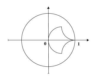
Figure 1: Cusp map domain

This map was first introduced in [11] (see also [13]). Explicitly, $\varphi$ is defined as follows.

We first map $\mathbb{D}$ onto the half-disk $\mathbb{D}^{+}=\{z\in\mathbb{D}\,;\ {\mathfrak{R}}{\rm e}\,z>0\}$. To do that, map $\mathbb{D}$ onto itself by $z\mapsto iz$; then map $\mathbb{D}$ onto the upper half-plane $\mathbb{H}=\{z\in\mathbb{C}\,;\ {\mathfrak{I}}{\rm m}\,z>0\}$ by:

$$T(u)=i\,\frac{1+u}{1-u}\,\cdot$$

Take the square root to map $\mathbb{H}$ in the first quadrant $Q_{1}=\{z\in\mathbb{H}\,;\ {\mathfrak{R}}{\rm e}\,z>0\}$, and go back to the half-disk $\{z\in\mathbb{D}\,;\ {\mathfrak{I}}{\rm m}\,z<0\}$ by $T^{-1}$: $T^{-1}(s)=\frac{1+is}{is-1}$; finally, make a rotation by $i$ to go onto $\mathbb{D}^{+}$. We get:

(4.1) $$\varphi_{0}(z)=\frac{\displaystyle\Big{(}\frac{z-i}{iz-1}\Big{)}^{1/2}-i}{\displaystyle-i\,\Big{(}\frac{z-i}{iz-1}\Big{)}^{1/2}+1}\,\cdot$$

One has $\varphi_{0}(1)=0$, $\varphi_{0}(-1)=1$, $\varphi_{0}(i)=-i$ and $\varphi_{0}(-i)=i$. The half-circle $\{z\in\mathbb{T}\,;\ {\mathfrak{R}}{\rm e}\,z\geq 0\}$ is mapped onto the segment $[-i,i]$ and the segment $[-1,1]$ onto the segment $[0,1]$.

Set now, successively,

(4.2) $$\varphi_{1}(z)=\log\varphi_{0}(z),\quad\varphi_{2}(z)=-\frac{2}{\pi}\,\varphi_{1}(z)+1,\quad\varphi_{3}(z)=\frac{1}{\varphi_{2}(z)}\,\raise 1.0pt\hbox{,}$$

and finally:

(4.3) $$\varphi(z)=1-\varphi_{3}(z)\,.$$

Hence:

(4.4) $$1-\varphi(z)=\frac{1}{1+\frac{2}{\pi}\,\log\big{(}1/|\varphi_{0}(z)|\big{)}-i\frac{2}{\pi}\arg\varphi_{0}(z)}\,\cdot$$

$\varphi_{2}$ maps $\mathbb{D}$ onto the semiband $\{z\in\mathbb{C}\,;\ {\mathfrak{R}}{\rm e}\,z>1\text{ and }|{\mathfrak{I}}{\rm m}\,z|<1\}$. One has $\varphi(1)=1$, $\varphi(-1)=0$, $\varphi(i)=(1+i)/2$ and $\varphi(-i)=(1-i)/2$.

The domain $\varphi(\mathbb{D})$ is edged by three circular arcs of radii $1/2$ and of respective centers $1/2$, $1+i/2$ and $1-i/2$. The real interval $]-1,1[$ is mapped onto the real interval $]\,0,1[$ and the half-circle $\{{\rm e}^{i\theta}\,;\ |\theta|\leq\pi/2\}$ is sent onto the two circular arcs tangent at $1$ to the real axis.

Lemma 4.2

1) For $0<r<1$, let $\gamma=\frac{\pi}{4}-\arctan r=\arctan[(1-r)/(1+r)]$; then:

(4.5) $$\varphi_{0}(r)=\tan(\gamma/2)\,.$$

Hence, when $r$ tends to $1_{-}$, one has:

(4.6) $$1-\varphi(r)\sim\frac{\pi}{2}\,\frac{1}{\log(1/\gamma)}\sim\frac{\pi}{2}\,\frac{1}{\log(1/(1-r))}\,\cdot$$

2) For $|\theta|<\pi/2$, one has:

(4.7) $$\varphi_{0}({\rm e}^{i\theta})=-i\,\frac{\tan(\theta/2)}{1+\sqrt{1-\tan^{2}(\theta/2)}}\,\cdot$$

Hence, when $\theta$ tends to $0$, one has:

(4.8) $$1-\varphi({\rm e}^{i\theta})\sim\frac{\pi}{2}\,\frac{1}{\log(1/|\theta|)}\,\cdot$$

Proof. 1) One has:

$$T(ir)=\frac{r-i}{ir-1}=-\frac{2r}{1+r^{2}}+i\,\frac{1-r^{2}}{1+r^{2}}=-\sin\alpha+i\cos\alpha\,,$$

with $r=\tan(\alpha/2)$; hence $T(ir)=\cos(\alpha+\pi/2)+i\sin(\alpha+\pi/2)={\rm e}^{i(\alpha+\pi/2)}$. Set $\beta=\frac{\alpha}{2}+\frac{\pi}{4}$; one gets:

$$\varphi_{0}(r)=\frac{{\rm e}^{i\beta}-i}{-i{\rm e}^{i\beta}+1}=\frac{\cos\beta}{1+\sin\beta}=\frac{\sin\gamma}{1+\cos\gamma}=\tan(\gamma/2)\,$$

with $\gamma=(\pi/2)-\beta=(\pi/4)-(\alpha/2)=(\pi/4)-\tan^{-1}r$. Then (4.6) follows.

2) Let $\tau=\frac{\pi}{2}-\theta$; one has:

$$T(i{\rm e}^{i\theta})=\frac{{\rm e}^{i\theta}-i}{i{\rm e}^{i\theta}-1}=\frac{-\cos\theta}{1+\sin\theta}=\frac{-\sin\tau}{1+\cos\tau}=-\tan(\tau/2).$$

Note that $0<\tau/2<\pi/2$ since $|\theta|<\pi/2$; hence $\tan(\tau/2)>0$. Therefore:

$$\varphi_{0}({\rm e}^{i\theta})=\frac{i\sqrt{\tan(\tau/2)}-i}{-i.i\sqrt{\tan(\tau/2)}+1}=i\,\frac{\sqrt{\tan(\tau/2)}-1}{\sqrt{\tan(\tau/2)}+1}\,\cdot$$

But

$$\tan(\tau/2)=\tan\Big{(}\frac{\pi}{4}-\frac{\theta}{2}\Big{)}=\frac{1-\tan(\theta/2)}{1+\tan(\theta/2)}\,;$$

it follows that:

$$\varphi_{0}({\rm e}^{i\theta}) =i\,\frac{\sqrt{1-\tan(\theta/2)}-\sqrt{1+\tan(\theta/2)}}{\sqrt{1-\tan(\theta/2)}+\sqrt{1+\tan(\theta/2)}}$$

$$=i\,\frac{\big{(}1-\tan(\theta/2)\big{)}-\big{(}1+\tan(\theta/2)\big{)}}{\big{(}\sqrt{1-\tan(\theta/2)}+\sqrt{1+\tan(\theta/2)}\big{)}^{2}}$$

$$=-i\,\frac{\tan(\theta/2)}{1+\sqrt{1-\tan^{2}(\theta/2)}}\,\cdot$$

Now, since $\varphi_{0}({\rm e}^{i\theta})\sim-i\theta/4$ as $\theta$ tends to $0$, we get (4.8). $\square$

It follows from this lemma and from Theorem 2.3 and Theorem 3.2 that one has the following estimate.

Theorem 4.3

For the approximation numbers $a_{n}(C_{\varphi})$ of the composition operator $C_{\varphi}\colon H^{2}\to H^{2}$ of symbol the cusp map $\varphi$, we have:

(4.9) $$\qquad\qquad\qquad\qquad{\rm e}^{-c_{1}\,n/\log n}\lesssim a_{n}(C_{\varphi})\lesssim{\rm e}^{-c_{2}\,n/\log n},\qquad\quad n=2,3,\ldots,$$

for some constants $c_{1}>c_{2}>0$.

Proof. 1) Upper estimate. Note first that, since the domain $\varphi(\mathbb{D})$ is contained in the right half-plane and in the symmetric angular sector of vertex $1$ and opening $\pi/2$, there is a constant $C>0$ such that $|1-\gamma(t)|\leq C\,(1-|\gamma(t)|)$ and we have (2.2). Then (4.8) in Lemma 4.2 gives (2.3). The upper estimate is hence given in Theorem 2.3 and (2.11).

2) Lower estimate. By Lemma 4.2, (4.6), one has (3.1). Since $\varphi$ is a real symbol, the upper estimate follows from Theorem 3.2, and (3.4). $\square$

4.2 The Shapiro-Taylor map

This one-parameter map $\varsigma_{\theta}\,$, $\theta>0$, was introduced by J. Shapiro and P. Taylor in 1973 ([22]) and was further studied, with a slightly different definition, in [9], Section 5. J. Shapiro and P. Taylor proved that $C_{\varsigma_{\theta}}\colon H^{2}\to H^{2}$ is always compact, but is Hilbert-Schmidt if and only if $\theta>2$. It is proved in [9], Theorem 5.1, that $C_{\varsigma_{\theta}}$ is in the Schatten class $S_{p}$ if and only if $p>4/\theta$.

Here, we shall use these maps $\varsigma_{\theta}$ to see the limitations of our previous methods.

We first recall their definition.

For $\varepsilon>0$, we set $V_{\varepsilon}=\{z\in\mathbb{C}\,;\ {\mathfrak{R}}{\rm e}\,z>0\text{ and }|z|<\varepsilon\}$. For $\varepsilon=\varepsilon_{\theta}>0$ small enough, one can define

(4.10) $$f_{\theta}(z)=z(-\log z)^{\theta},$$

for $z\in V_{\varepsilon}$, where $\log z$ will be the principal determination of the logarithm. Let now $g_{\theta}$ be the conformal mapping from $\mathbb{D}$ onto $V_{\varepsilon}$, which maps $\mathbb{T}=\partial\mathbb{D}$ onto $\partial V_{\varepsilon}$, defined by $g_{\theta}(z)=\varepsilon\,\varphi_{0}(z)$, where $\varphi_{0}$ is given in (4.1).

Then, we define:

(4.11) $$\varsigma_{\theta}=\exp(-f_{\theta}\circ g_{\theta}).$$

One has $\varsigma_{\theta}(1)=1$ and $g_{\theta}({\rm e}^{it})\sim-it/4$ as $t$ tends to $0$, by Lemma 4.2; hence, when $t$ is near of $0$:

$$|1-\varsigma_{\theta}({\rm e}^{it})|\approx|f_{\theta}[g_{\theta}({\rm e}^{it})]|\approx|t|\,[\log(1/|t|)]^{\theta}.$$

If we were allowed to apply Theorem 2.3, we would get that $a_{n}(C_{\varsigma_{\theta}})\lesssim 1/n^{\theta/4}$, which would be in accordance with the fact that $C_{\varsigma_{\theta}}$ is in the Schatten class $S_{p}$ if and only if $p>4/\theta$. However, condition (2.2) is not satisfied: by [9], equations (5.5) and (5.6), one has $1-|\varsigma_{\theta}({\rm e}^{it})|\approx|t|(\log 1/|t|)^{\theta-1}$, whereas $|1-\varsigma_{\theta}({\rm e}^{it})|\approx|t|(\log 1/|t|)^{\theta}$.

On the other hand, by the Lemma 4.2 again, $g_{\theta}(r)\sim\varepsilon(1-r)/4$ as $r$ tends to $1$; hence, when $r$ is near to $1$:

$$1-\varsigma_{\theta}(r)\approx(1-r)\big{(}\log 1/(1-r)\big{)}^{\theta},$$

so $\varsigma_{\theta}$ is a real $\omega$-radial symbol with $\omega(t)=t(\log 1/t)^{\theta}$. Hence, we get from Theorem 3.2:

$$a_{n}(C_{\varsigma_{\theta}})\gtrsim\frac{1}{n^{\theta/2}}\,\raise 1.0pt\hbox{,}$$

taking $\sigma=1/{\rm e}$ in (3.2). However, this lower estimate is not the right one, since $C_{\varsigma_{\theta}}$ is in $S_{p}$ if and only if $p>4/\theta$.

5 Contact points

It is well-known (and easy to prove) that for every compact composition operator $C_{\varphi}\colon H^{2}\to H^{2}$, the set of contact points

$$E_{\varphi}=\{{\rm e}^{i\theta}\,;\ |\varphi^{\ast}({\rm e}^{i\theta})|=1\}$$

has Lebesgue measure $0$. A natural question is: to what extent is this negligible set arbitrary? The following partial answer was given by E.A. Gallardo-Gutiérrez and M.J. González in [6].

Theorem 5.1 (E.A. Gallardo-Gutiérrez and M.J. González)

There is a compact composition operator $C_{\varphi}$ on $H^{2}$ such that the Hausdorff dimension of $E_{\varphi}$ is one.

This was generalized by O. El-Fallah, K. Kellay, M. Shabankhah, and H. Youssfi ([5], Theorem 3.1):

Theorem 5.2 (O. El-Fallah, K. Kellay, M. Shabankhah, H. Youssfi)

For every compact set $K$ of measure $0$ in $\mathbb{T}$, there exists a Schur function $\varphi\in A(\mathbb{D})$, the disk algebra, such that the associated composition operator $C_{\varphi}$ is Hilbert-Schmidt on $H^{2}$ and $E_{\varphi}=K$.

As an application of our previous results, we shall extend these results, with a very simple proof. Our composition operator will not even be compact, or Hilbert-Schmidt, but in all Schatten classes $S_{p}$, and moreover its approximation numbers will be as small as possible.

Theorem 5.3

Let $K$ be a Lebesgue-negligible compact set of the circle $\mathbb{T}$. Then, there exists a Schur function $\psi\in A(\mathbb{D})$, the disk algebra, such that $E_{\psi}=K$, $\psi({\rm e}^{i\theta})=1$ for all ${\rm e}^{i\theta}\in K$, and:

(5.1) $$a_{n}(C_{\psi})\leq a\exp(-b\,n/\log n).$$

In particular, $C_{\psi}\in\bigcap_{p>0}S_{p}$.

Proof. According to the Rudin-Carleson theorem ([2]), we can find $\chi\in A(\mathbb{D})$ such that

$$\qquad\chi=1\text{ on }K\quad\text{and}\quad|\chi|<1\text{ on }\overline{\mathbb{D}}\setminus K.$$

Consider now the cusp map $\varphi$, defined in Section 4.1. One has $\varphi\in A(\mathbb{D})$, $\varphi(1)=1$ and

$$a_{n}(C_{\varphi})\leq a^{\prime}\exp(-b\,n/\log n).$$

We now spread the point $1$ by composing with the function $\chi$, which is equal to $1$ on the whole of $K$. We check that the composed map $\psi=\varphi\circ\chi$ has the required properties.

That $\psi\in A(\mathbb{D})$ is clear. For $z\in K$, one has $\psi(z)=\varphi(1)=1$, and for $z\in\overline{\mathbb{D}}\setminus K$, one has $|\chi(z)|<1$; hence $|\psi(z)|<1$.

To finish, since $C_{\psi}=C_{\chi}\circ C_{\varphi}$, we have

$$a_{n}(C_{\psi})\leq\|C_{\chi}\|\,a_{n}(C_{\varphi})\leq a^{\prime}\,\|C_{\chi}\|\,\exp(-b\,n/\log n):=\sigma_{n},$$

proving the result (with $a=a^{\prime}\,\|C_{\chi}\|$), since clearly $\sum_{n=1}^{\infty}\sigma_{n}^{p}<\infty$ for each $p>0$. $\square$

Actually, we can improve on the previous theorem by proving the following result. This result is optimal because if $\|\psi\|_{\infty}=1$, we know (see [14], Theorem 3.4) that $\liminf_{n\to\infty}[a_{n}(C_{\psi})]^{1/n}=1$, so we cannot hope to get rid with the forthcoming vanishing sequence $(\varepsilon_{n})_{n}$.

Theorem 5.4

Let $K$ be a Lebesgue-negligible compact set of the circle $\mathbb{T}$ and $(\varepsilon_{n})_{n}$ a sequence of positive real numbers with limit zero. Then, there exists a Schur function $\varphi\in A(\mathbb{D})$ such that $E_{\varphi}=K$, $\varphi({\rm e}^{i\theta})=1$ for all ${\rm e}^{i\theta}\in K$, and

(5.2) $$a_{n}(C_{\varphi})\leq C\exp(-n\,\varepsilon_{n})\,,$$

where $C$ is a positive constant.

This theorem is a straightforward consequence of the following lemma. Recall that the Carleson function of the Schur function $\psi\colon\mathbb{D}\to\mathbb{D}$ is defined by:

$$\rho_{\psi}(h)=\sup_{|\xi|=1}m(\{t\in\mathbb{T}\,;\ |\psi({\rm e}^{it})|\geq 1-h\text{ and }|\arg(\psi({\rm e}^{it})\,\bar{\xi})|\leq\pi h\}).$$

Lemma 5.5

Let $\delta$ be a nondecreasing positive function on $(0,1]$ tending to $0$ as $h\to 0$. Then, there exists a Schur function $\psi\in A(\mathbb{D})$ such that $\psi(1)=1$, $|\psi(\xi)|<1$ for $\xi\in\mathbb{T}\setminus\{1\}$, and such that $\rho_{\psi}(h)\leq\delta(h)$, for $h>0$ small enough.

Once we have the lemma, in view of the upper bound in [14], Theorem 5.1, for approximation numbers, we can adjust the function $\delta$ so as to have $a_{n}(C_{\psi})\leq K{\rm e}^{-n\varepsilon_{n}}$. Then, we compose $\psi$ with a peaking function $\chi$ as in the previous section and the map $\varphi=\psi\circ\chi$ fulfills the requirements of Theorem 5.4, with $C=K\|\chi\|$. $\square$

Proof of Lemma 5.5. We use a slight modification of the map $g$ constructed in [10], pages 66–67. Instead of taking a conformal map from $\mathbb{D}$ to the domain used in [10], we modify this domain by limiting it to the right- hand side (by, say, a semicircle), as on the Figure 2. Let $\Omega$ this domain. This domain is limited by the two hyperbolas $y=1/x$ and $y=(1/x)+4\pi$. The limiting semicircle is chosen in order that ${\mathfrak{I}}{\rm m}\,w\geq 1$ for $w\in\Omega$. The lower part of the “saw-teeth” have an imaginary part equal to $4\pi n$. If $a\in\Omega$ is fixed and $\Omega_{n}$ is the part of the domain $\Omega$ such that ${\mathfrak{I}}{\rm m}\,w<4\pi n$, the horizontal sizes of the “saw-teeth” are chosen in order that the harmonic measure $\omega_{\Omega}(a,\partial\Omega\setminus\partial\Omega_{n})$ is $\leq\delta_{n}:=\delta(1/16\pi(n+1))$. Note that $\partial\Omega\setminus\partial\Omega_{n}\supseteq\{w\in\partial\Omega\,;\ {\mathfrak{I}}{\rm m}\,w>4\pi n\}$ (see [10], Lemma 4.2).

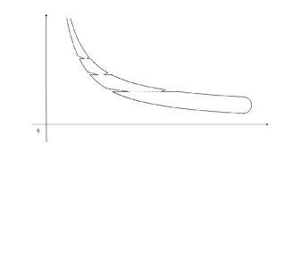
Figure 2: Domain $\Omega$

By Carathéodory-Osgood’s Theorem (see [20], Theorem IX.4.9), there is a unique homeomorphism $g$ from $\overline{\mathbb{D}}$ onto $\overline{\Omega}\cup\{\infty\}$ which maps conformally $\mathbb{D}$ onto $\Omega$ and such that $g(0)=a$ and $g(1)=\infty$ (we may choose these two values because if $h\colon\overline{\mathbb{D}}\to\overline{\Omega}\cup\{\infty\}$ is such a map, and $u$ is the automorphism of $\overline{\mathbb{D}}$ such that $u(0)=h^{-1}(a)$ and $u(1)=h^{-1}(\infty)$, then $g=h\circ u$ suits – alternatively, having choosen $h(0)=a$, then, if $h({\rm e}^{i\theta_{0}})=\infty$, we take $g(z)=h({\rm e}^{i\theta_{0}}z)$).

We define $\psi=(g-i)/(g+i)$. Then $\psi\colon\mathbb{D}\to\mathbb{D}$ is a Schur function and $\psi\in A(\mathbb{D})$. Moreover, since the domain $\Omega$ is bounded horizontally, we have $\psi(1)=1$ and $|\psi({\rm e}^{it})|<1$ for $0<t<2\pi$.

Now, $\rho_{\psi}(h)\leq m\big{(}\{z\in\mathbb{T}\,;\ |\psi(z)|>1-h\}\big{)}$. Writing $g=u+iv$, one has:

$$|\psi|^{2}=\frac{u^{2}+(v-1)^{2}}{u^{2}+(v+1)^{2}}=1-\frac{4v}{u^{2}+(v+1)^{2}}\,\cdot$$

Since $(1-h)^{2}\geq 1-2h$, the condition $|\psi(z)|>1-h$ implies that $\frac{2v}{u^{2}+(v+1)^{2}}\leq h$. But $0<u\leq 1+2\pi\leq 8$ and $(v+1)^{2}\leq 4v^{2}$ (since $v\geq 1$); we get hence $\frac{v}{32+2v^{2}}\leq h$, or $\frac{32}{v}+2v\geq\frac{1}{h}$. Using again the fact that $v\geq 1$, one obtains $2v\geq\frac{1}{h}-32$, and hence $2v\geq\frac{1}{2h}$ for $0<h\leq 1/64$. Therefore, for $0<h\leq 1/64$,

$$\rho_{\psi}(h)\leq m(\{z\in\mathbb{T}\,;\ {\mathfrak{I}}{\rm m}\,\psi(z)\geq 1/4h\})\,.$$

Now, for $n\geq 2$ and $1/16\pi(n+1)\leq h<1/16\pi n$, one gets hence:

$$\rho_{\psi}(h) \leq m(\{z\in\mathbb{T}\,;\ {\mathfrak{I}}{\rm m}\,\psi(z)>4\pi n\})$$

$$=\omega_{\Omega}(a,\{w\in\partial\Omega\,;\ {\mathfrak{I}}{\rm m}\,w>4\pi n\})\leq\omega_{\Omega}(a,\partial\Omega\setminus\partial\Omega_{n})\leq\delta_{n}\leq\delta(h)\,,$$

proving Lemma 5.5. $\square$

Daniel Li, Univ Lille Nord de France, U-Artois,
Laboratoire de Mathématiques de Lens EA 2462 & Fédération CNRS Nord-Pas-de-Calais FR 2956,
Faculté des Sciences Jean Perrin, Rue Jean Souvraz, S.P.18,
F-62300 LENS, FRANCE
daniel.li@euler.univ-artois.fr

Hervé Queffélec, Univ Lille Nord de France,
USTL, Laboratoire Paul Painlevé U.M.R. CNRS 8524,
Fédération CNRS Nord-Pas-de-Calais FR 2956,
F-59655 VILLENEUVE D’ASCQ Cedex, FRANCE
Herve.Queffelec@univ-lille1.fr

Luis Rodríguez-Piazza, Universidad de Sevilla,
Facultad de Matemáticas, Departamento de Análisis Matemático & IMUS,
Apartado de Correos 1160,
41080 SEVILLA, SPAIN
piazza@us.es