Reduction of interaction delays in networks
[appeared in EPL, 103 (2013) 10006, DOI:10.1209/0295-5075/103/10006]

Abstract

Delayed interactions are a common property of coupled natural systems and therefore arise in a variety of different applications. For instance, signals in neural or laser networks propagate at finite speed giving rise to delayed connections. Such systems are often modeled by delay differential equations with discrete delays. In realistic situations, these delays are not identical on different connections. We show that by a componentwise timeshift transformation it is often possible to reduce the number of different delays and simplify the models without loss of information. We identify dynamic invariants of this transformation, determine its capabilities to reduce the number of delays and interpret these findings in terms of the topology of the underlying graph. In particular, we show that networks with identical sums of delay times along the fundamental semicycles are dynamically equivalent and we provide a normal form for these systems. We illustrate the theory using a network motif of coupled Mackey-Glass systems with 8 different time delays, which can be reduced to an equivalent motif with three delays.

¹ Humboldt-University of Berlin, Institute of Mathematics, Unter den Linden 6, 10099 Berlin, Germany.
² Université Montpellier 2, Institut de Mathématiques et de Modélisation de Montpellier (I3M), Place Eugène Bataillon, 34095 Montpellier Cedex, France.

1 Introduction

Time delays play an important role in the realistic modeling of networks of dynamical systems. For instance, in gene regulatory networks delayed couplings arise due to the finite duration of biochemical reaction chains [1, 2, 3, 4, 5, 6], in population dynamics due to the processes of maturation and gestation [7], and in laser networks they correspond to the propagation time of light between interacting lasers [8, 9, 10, 11]. Similarly, in neuronal networks delays occur due to the finite propagation times of action potentials along the axons or to reaction times at chemical synapses [12, 13, 14, 15, 16, 17]. Depending on the physiological properties of axons and synapses, the delays of signals between different cells in the network differ and in practice there are as many different delays in the network as there are links between single neurons. Such a diversity of delays was shown to enable the design of robust pattern generating systems [18, 19] and to play an important role in neural processing of spatio-temporal information [20]. On a mesoscopic level, networks of neuronal populations responsible for motor control and human cognition involve transmission delays depending on the locations of the populations in the brain [21, 22]. Hence, to study such natural systems, one would need to study models involving numerous different delays. Independently of the physical origin, dynamics in networks of $N$ interacting systems can often be described by the equations

$$\dot{\boldsymbol{x}}_{j}(t)=f_{j}\left(\boldsymbol{x}_{j}(t),\boldsymbol{x}_{1}\left(t-\tau_{j1}\right),\dots,\boldsymbol{x}_{N}\left(t-\tau_{jN}\right)\right),$$ (1)

where $\boldsymbol{x}_{j}(t)\in\mathbb{R}^{n_{j}}$, $1\leq j\leq N$, denotes the state of the node $j$ and $\tau_{jk}\geq 0$ is the time delay, which occurs due to the signal propagation time from a node $k$ to the node $j$. For instance, $\boldsymbol{x}_{j}$ may be considered as a variable describing the dynamics of one neuron in the network and $\tau_{jk}$ as the time which an action potential needs to travel along the axon of neuron $\boldsymbol{x}_{k}$ until it arrives at the synapse connecting it to $\boldsymbol{x}_{j}$. Equation (1) includes the possibility of an all-to-all coupling structure. However, in many situations, the coupling is not global and $\boldsymbol{x}_{j}$ receives direct inputs from only relatively few other nodes. Therefore, we consider the set $P_{j}$ of all nodes of the network, which are connected to the node $j$ and write system (1) in a more compact, equivalent form

$$\dot{\boldsymbol{x}}_{j}(t)=f_{j}\left(\boldsymbol{x}_{j}(t),\left(\boldsymbol{x}_{k}\left(t-\tau_{jk}\right)\right)_{k\in P_{j}}\right).$$ (2)

The only difference of the form of writing (2) from the general form (1) is that is explicitly shows which connections are present in the network. Throughout what follows, we consider directed networks, thus one may generally have $\tau_{jk}\neq\tau_{kj}$ or even $k\in P_{j}$ while $j\notin P_{k}$. Moreover, we assume that the network is connected and hence, the number $L$ of links is at least $N-1$. In fact, the obtained results hold also for networks with multiple links between the nodes, but we discuss only systems of the form (2) in order to avoid complicated notations. For a network of $N$ systems, up to $N^{2}$ different time delays may occur in (2). This creates immense challenges for the analysis of the system, since every single delay may alter the properties and dynamics significantly [23, 24, 25, 26, 27, 28, 29].

In this Letter we show how the number of different delays can be reduced. It appears that any connected network (2) possesses a characteristic number of delays which are essential for describing the dynamics. This number of essential delays equals the cycle space dimension $C=L-\left(N-1\right)$ of the underlying graph and is usually smaller than the number of distinct $\tau_{jk}$. We show that the essential delays correspond to the sums of the delay times along fundamental semicycles (cycles in the underlying undirected graph) in the network. As we explain below, networks which have the same local dynamics and the same set of essential delays can be considered as equivalent from the dynamical point of view. Our results represent fundamental theoretical insights which help to understand delay coupled systems. For instance, they can be used to simplify bifurcation analysis when varying one or several delays or to speed up numerical simulations of delay equations.

1.1 Reduction of delays in unidirectional rings

As a simple illustrative example, let us consider a ring of unidirectionally coupled systems

$$\dot{\boldsymbol{x}}_{j}\left(t\right)=f\left(\boldsymbol{x}_{j}\left(t\right),\boldsymbol{x}_{j+1}\left(t-\tau_{j}\right)\right),$$ (3)

with inhomogeneous coupling delays $\tau_{j}$, $\ 1\leq j\leq N$, and periodic indices, i.e., $\boldsymbol{x}_{N+1}=\boldsymbol{x}_{1}$. It is known [30, 31] that this system can be reduced to a ring where all time delays are equal to $\tau=\frac{1}{N}\sum\tau_{j}$. This can be done by a componentwise timeshift transformation for each node

$$\boldsymbol{y}_{j}\left(t\right)=\boldsymbol{x}_{j}\left(t+\eta_{j}\right),\quad 1\leq j\leq N.$$ (4)

Indeed, the transformed variables $\boldsymbol{y}_{j}\left(t\right)$ fulfill

$$\dot{\boldsymbol{y}}_{j}\left(t\right)=f\left(\boldsymbol{y}_{j}\left(t\right),\boldsymbol{y}_{j+1}\left(t-\tau_{j}+\eta_{j}-\eta_{j+1}\right)\right).$$ (5)

This means that the timeshift transformation (4) formally allows to change the delays as $\tau_{j}\mapsto\tilde{\tau}_{j}=\tau_{j}-\eta_{j}+\eta_{j+1}$. If the shifts $\eta_{j}$ are chosen appropriately, all hitherto distinct delays become the same while their sum along the ring, the roundtrip time $N\tau$, is preserved. It is clear that both systems, (3) and (5), possess the same steady states and there is a one-to-one correspondence of periodic solutions via (4). However, previous studies using this type of transformation did not attempt to show in which sense (2) and (5) are dynamical equivalent nor did they explore how the method generalizes to more complex networks. Our aim is to treat these questions and apply the timeshift transformation (4) to reduce the number of different delays in networks with arbitrary topology.

2 Reduction of delays in general coupling structures

Applying the transformation (4) to a system of the form (2), we obtain the new system

$$\dot{\boldsymbol{y}}_{j}\left(t\right)=f_{j}\left(\boldsymbol{y}_{j}\left(t\right),\left(\boldsymbol{y}_{k}\left(t-\tilde{\tau}_{jk}\right)\right)_{k\in P_{j}}\right)$$ (6)

with the modified delays $\tilde{\tau}_{jk}=\tau_{jk}+\eta_{k}-\eta_{j}$. As for the unidirectional ring (3), also in arbitrary networks the roundtrip times along closed paths remain unchanged by the componentwise timeshift transformation. In order to formulate this general principle more precisely, we use two definitions. A semicycle in a directed graph is a set $c=\{\ell_{1},...,\ell_{k}\}$ of links $\ell_{j}$, which constitute a cycle when neglecting their directionality. For example, in the network displayed in fig. 2 the links along the path STN$\rightarrow$GPe$\rightarrow$STN constitute a semicycle, but also those of GPe$\rightarrow$STN$\rightarrow$GPi$\leftarrow$GPe. The roundtrip time along a semicycle $c$ is defined as

$$T\left(c\right):=\Big{|}\sum_{j=1}^{k}\sigma_{j}\tau\left(\ell_{j}\right)\Big{|},$$ (7)

where $\tau\left(\ell_{j}\right)$ is the time delay along the link $\ell_{j}$ and $\sigma_{j}$ is either $+1$ or $-1$ depending on the direction of the link $\ell_{j}$ with respect to an arbitrary but fixed orientation of the semicycle. For example, the roundtrip of the semicycle GPe$\overset{\tau_{2}}{\rightarrow}$STN$\overset{\tau_{3}}{\rightarrow}$GPi$\overset{\tau_{4}}{\leftarrow}$GPe in fig. 2 is $T=|\tau_{2}+\tau_{3}-\tau_{4}|$. Note that the orientation can be chosen in two different ways, which corresponds to opposite signs of $\sigma_{j}$. However, the obtained value for $T\left(c\right)$ is independent of the choice of orientation. Most importantly, the roundtrip time stays invariant under the componentwise timeshift transformation, i.e.,

$$\tilde{T}\left(c\right)=\Big{|}\sum_{j=1}^{k}\sigma_{j}\tilde{\tau}\left(\ell_{j}\right)\Big{|}=T\left(c\right),$$ (8)

where $\tilde{\tau}(\ell)$ is the transformed delay on the link $\ell$. Denoting the source of $\ell$ by $s(\ell)$ and its target by $t(\ell)$, we have $\tilde{\tau}(\ell)=\tau(\ell)+\eta_{s(\ell)}-\eta_{t(\ell)}$. On the other hand, for any choice of delays $\tilde{\tau}(\ell)$ which preserves the roundtrips, there exist corresponding timeshifts $\eta_{j}$ such that $\tilde{\tau}(\ell)=\tau(\ell)+\eta_{s(\ell)}-\eta_{t(\ell)}$. This equivalence provides an intuitive way of looking for possible transformations in simple networks: One can redistribute delays as long as the roundtrips stay fixed.

2.1 Construction of a delay-free spanning tree

In the following, we explain how to construct timeshifts $\eta_{j}$ such that the transformed network (6) has a minimal number of delayed connections. Simultaneously with the timeshifts, we construct a set $S=\left\{\ell_{1},...,\ell_{N-1}\right\}$ of $N-1$ links, such that the transformed delays $\tilde{\tau}(\ell)$ are zero on all links from $S$ and non-negative on all other links. In fact, the set $S$ is a spanning tree: a set of $N-1$ links which does not contain any semicycle. Each node of the network occurs at least once as a target or source of some link in $S$, and the addition of any link $\ell\notin S$ results in a set $S^{\prime}=S\cup\left\{\ell\right\}$, which contains exactly one semicycle. This is the fundamental semicycle corresponding to $\ell$ with respect to $S$. The transformed delay $\tilde{\tau}\left(\ell\right)$ on the link $\ell$ equals the roundtrip time of this fundamental semicycle. Consequently, the number of delays in the transformed system can be reduced to

$$C=L-N+1,$$ (9)

where $L$ is the number of links in the network. The resulting system, whose links are instantaneous along $S$, may function as a normal form for the class of equivalent systems which exhibit the same roundtrips along their semicycles.

To construct the appropriate timeshifts and the spanning tree $S$, we proceed iteratively. Firstly, we select a spanning tree $S_{0}=\{\ell_{1}^{0},...,\ell_{N-1}^{0}\}$ in the following way: $\ell_{1}^{0}$ is chosen as a link with the minimal delay and successive elements $\ell_{j}^{0}$ are always chosen to have minimal possible delay, such that $\{\ell_{1}^{0},...,\ell_{j}^{0}\}$ remains cycle free. As a next step consider the link $\ell\in S_{0}$ with minimal non-zero delay $\tau(\ell)>0$ (it equals $\ell_{1}^{0}$ if $\tau(\ell_{1}^{0})>0$). As depicted in fig. 1, the link $\ell$ divides $S_{0}$ in two connected parts: one either being empty or containing at least one link connecting to the source $s(\ell)$ of $\ell$, the other being empty or connecting its target $t(\ell)$ with other nodes. Correspondingly, the nodes are also divided into two sets $V$ and $W$ with $s(\ell)\in V$ and $t(\ell)\in W$.

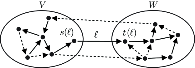
Figure 1: Illustration of the partition of the network into two sets $V$ and $W$, which is induced by a link $\ell$ contained in a spanning tree $S$ (solid links). Links which are not contained in the spanning tree are indicated by dashed lines.

An application of the timeshift transformation with $\eta_{j}=\tau(\ell)$ for all $j\in W$, and $\eta_{j}=0$ for $j\in V$, yields $\tilde{\tau}(\ell)=\tau(\ell)+\eta_{s(\ell)}-\eta_{t(\ell)}=0$. All other delays on links in $S_{0}$ remain unchanged because for links which connect nodes from the same set $V$ or $W$ there is no difference in the timeshifts and therefore no change of delays. By construction of $S_{0}$, any link $\ell^{\prime}\notin S_{0}$, which connects $V$ and $W$, must satisfy $\tau(\ell^{\prime})\geq\tau(\ell)$. Otherwise, $\ell^{\prime}$ had been added to $S_{0}$ instead of $\ell$. Therefore, we have $\tilde{\tau}(\ell^{\prime})=\tau(\ell^{\prime})+\eta_{s(\ell^{\prime})}-\eta_{t(\ell^{\prime})}\geq\tau(\ell^{\prime})-\tau(\ell)\geq 0$. Hence, delays on links which are not contained in $S_{0}$ cannot become negative. A successive spanning tree $S_{1}$, which contains at least one more instantaneous link is obtained by keeping all instantaneous links from $S_{0}$ and then adding links in the same manner as above. Proceeding in this fashion produces a completely instantaneous spanning tree $S$ in less than $N$ steps.

After the above reduction, the number of different delays is not larger than $C=L-N+1$. Since $C$ is the minimal number of different delays which can be achieved generically, we call it the essential number of delays. Here, "generically" means that the set of delays, which allow to reduce the number of different delays to less than $C$, is a set of measure zero in the parameter space $\mathbb{R}^{L}_{\geq 0}$. $C$ has a well known meaning for network graphs [32]: It is the cycle space dimension which is defined as the maximal number of independent cycles. A set of cycles is called independent if none of the cycles can be obtained as a sum of the other cycles in the set. Here, the sum of two cycles $c_{1}$ and $c_{2}$ is defined as the symmetric difference $c_{1}\bigtriangleup c_{2}=(c_{1}\cup c_{2})\setminus(c_{1}\cap c_{2})$. For instance, in the network given in fig. 3 the cycle space dimension is $C=3$.

2.2 A two-cycle neuronal network

Let us illustrate the main ideas of the reduction with an examplary network structure which resembles the connections between several areas in the brain (see fig. 2): the subthalamic nucleus (STN), the external segment (GPe), and the internal segment (GPi) of the globus pallidus [33, 34]. Additional external inputs from the thalamus and cortex (ThCx) arrive at the STN. We denote the different areas by $\boldsymbol{x}_{1}$ (STN), $\boldsymbol{x}_{2}$ (GPe), $\boldsymbol{x}_{3}$ (GPi), and $\boldsymbol{x}_{4}$ (ThCx). As general form of the equations which may describe the corresponding dynamics, we assume

$$\dot{\boldsymbol{x}}_{1}\left(t\right) =f_{1}\left(\boldsymbol{x}_{1}\left(t\right),\boldsymbol{x}_{2}\left(t-\tau_{2}\right),\boldsymbol{x}_{4}\left(t-\tau_{5}\right)\right),$$ (10)

$$\dot{\boldsymbol{x}}_{2}\left(t\right) =f_{2}\left(\boldsymbol{x}_{2}\left(t\right),\boldsymbol{x}_{1}\left(t-\tau_{1}\right)\right),$$

$$\dot{\boldsymbol{x}}_{3}\left(t\right) =f_{3}\left(\boldsymbol{x}_{3}\left(t\right),\boldsymbol{x}_{1}\left(t-\tau_{3}\right),\boldsymbol{x}_{2}\left(t-\tau_{4}\right)\right),$$

$$\dot{\boldsymbol{x}}_{4}\left(t\right) =f_{4}\left(\boldsymbol{x}_{4}\left(t\right),\boldsymbol{x}_{4}\left(t-\tau_{6}\right)\right),$$

with connection delays $\tau_{j}>0$.

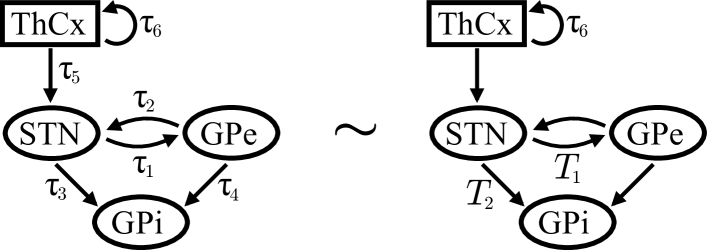
Figure 2: A small network with four nodes and two cycles corresponding to eqs. (10) which resemble the connectivity between several regions in the brain [see main text]. The componentwise timeshift transformation (4) leads from the original system (left) to a system with a reduced number of delays (right), where $T_{1}=\tau_{1}+\tau_{2}$ and $T_{2}=\tau_{2}+\tau_{3}-\tau_{4}$.

The transformation (4) leads to new delays

$$\tilde{\tau}_{1}=\tau_{1}-\eta_{2}+\eta_{1},\ \tilde{\tau}_{2}=\tau_{2}-\eta_{1}+\eta_{2},\ \tilde{\tau}_{3}=\tau_{3}-\eta_{3}+\eta_{1},\\ \tilde{\tau}_{4}=\tau_{4}-\eta_{3}+\eta_{2},\ \tilde{\tau}_{5}=\tau_{5}-\eta_{1}+\eta_{4},\text{ and }\tilde{\tau}_{6}=\tau_{6}.$$

The roundtrips $T_{1}:=\tau_{1}+\tau_{2}$ and $T_{2}:=\tau_{2}+\tau_{3}-\tau_{4}$ are invariant: they stay the same for the new delays. In particular, this implies that a reduction to one delay, which was possible for the ring, cannot be achieved in general. There exist 6 formal possibilities to reduce the four different delays $\tau_{1-4}$ of (10) to two by an appropriate choice of $\eta_{1-3}$ [see Table 1]. However, some reductions should be excluded because they lead to negative delays in the resulting network. Such ”anticipating arguments” create functional differential equations of mixed type. We avoid this case because for these equations the initial value problem is usually ill-posed [35]. As a result of the reduction, an equivalent system [fig. 2, right panel] contains only three time delays: the self-feedback $\tau_{6}$ to the ThCx, the short roundtrip delay $T_{1}$ between STN and GPe, and the roundtrip $T_{2}$ along the STN $\to$ GPe $\to$ GPi connection. The example illustrates also several general principles. Firstly the delays of self-couplings cannot be eliminated (e.g. $\tilde{\tau}_{6}=\tau_{6}$). Further, one may always choose $\eta_{4}=\eta_{1}-\tau_{5}$, such that $\tilde{\tau}_{5}=0$. That is, delays on leaves (nodes with only one link to others) may be neglected.

$\tilde{\tau}_{1}$	$\tilde{\tau}_{2}$	$\tilde{\tau}_{3}$	$\tilde{\tau}_{4}$	$\tilde{\tau}_{5}$	$\tilde{\tau}_{6}$
$T_{1}$	0	0	$-T_{2}$	0	$\tau_{6}$
$T_{1}$	0	$T_{2}$	0	0	$\tau_{6}$
0	$T_{1}$	$T_{2}-T_{1}$	0	0	$\tau_{6}$
0	$T_{1}$	0	$T_{1}-T_{2}$	0	$\tau_{6}$
$T_{1}/2$	$T_{1}/2$	$T_{2}-T_{1}/2$	0	0	$\tau_{6}$
$T_{1}/2$	$T_{1}/2$	0	$T_{1}/2-T_{2}$	0	$\tau_{6}$

Table 1: Possible delay reductions in the network [fig. 2, eqs. (10)] under the condition $\tilde{\tau}_{5}=0$. The two roundtrips $T_{1}=\tau_{1}+\tau_{2}$ and $T_{2}=\tau_{2}+\tau_{3}-\tau_{4}$ were used to parametrize the different combinations for $\tilde{\tau}_{1-4}$. The spanning tree algorithm [see main text] produces one of the first four possibilities depending on the values of $\tau_{1-4}$.

Let us give a brief explanation of how the algorithm works in the present example with delay times $\tau_{1}=1$, $\tau_{2}=2$, $\tau_{3}=3$, $\tau_{4}=4$, and $\tau_{5}=5$ For this choice we find that $T_{1}=3$ and $T_{2}=1$. Let us denote the links by $\ell_{1-5}$ such that $\tau(\ell_{j})=\tau_{j}$. The initial spanning tree is then $S_{0}=\{\ell_{1},\ell_{3},\ell_{5}\}$. Note that, although $\tau_{2}<\tau_{3}$, the link $\ell_{2}$ cannot be added to $S_{0}$ instead of $\ell_{3}$ because this would result in a cycle $\{\ell_{1},\ell_{2}\}$. Similarly, $\ell_{5}$ is added instead of $\ell_{4}$. In the next step, the sets $V=\{\boldsymbol{x}_{1},\boldsymbol{x}_{3},\boldsymbol{x}_{4}\}$ and $W=\{\boldsymbol{x}_{2}\}$ are formed and the delay $\tau_{1}$ is eliminated by a timeshift transformation with $\eta_{1}=\eta_{3}=\eta_{4}=0$ and $\eta_{2}=\tau_{1}=1$. This results in transformed delays $\tilde{\tau}_{1}=0$, $\tilde{\tau}_{2}=\tilde{\tau}_{3}=3$, and $\tilde{\tau}_{4}=\tilde{\tau}_{5}=5$. The successive spanning tree has to be chosen as before $S_{1}=S_{0}$. The smallest non-zero delay on $S_{1}$ is now $\tilde{\tau}_{3}=3$ and correspondingly we set $V=\{\boldsymbol{x}_{1},\boldsymbol{x}_{2},\boldsymbol{x}_{4}\}$ and $W=\{\boldsymbol{x}_{3}\}$. An application of the timeshift transformation with $\eta_{1}=\eta_{2}=\eta_{4}=0$ and $\eta_{3}=3$ eliminates the delay on $\ell_{3}$ and we obtain: $\tilde{\tilde{\tau}}_{1}=\tilde{\tilde{\tau}}_{3}=0$, $\tilde{\tilde{\tau}}_{2}=3$, $\tilde{\tilde{\tau}}_{4}=2$, and $\tilde{\tilde{\tau}}_{5}=5$. For the final step, we find $S_{2}=S_{0}$, $V=\{\boldsymbol{x}_{4}\}$, $W=\{\boldsymbol{x}_{1-3}\}$ and, applying the timeshift-transform with $\eta_{4}=0$ and $\eta_{1-3}=5$ gives the reduced delay distribution which is listed in the fourth row of Table 1.

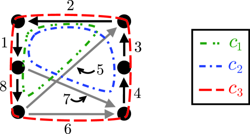
Figure 3: A network of $N=6$ systems with cycle space dimension $C=3$. A spanning tree [black links], three fundamental links [grey links] and three corresponding fundamental cycles [see legend], are shown. The numbers refer to the indexing of the links which is used in the text. According to our results, any admissible dynamics in this network involves at most three different interaction delays.

3 Dynamical invariants

As mentioned above, it is possible to create negative delays $\tilde{\tau}_{jk}$ by certain choices of the timeshifts $\eta_{j}$. This would change the type of the problem fundamentally. At least for this reason it is worth considering to what extent the systems (2) and (6) possibly differ in their dynamical behavior. Fortunately, negative delays turn out to be the only pathological case, as we show in the following. More precisely, we show that characteristic exponents of steady states and periodic solutions are the same in both systems. This implies that the linear stability of these solutions is the same [35]. Firstly, we consider a steady state $\boldsymbol{x}^{\ast}=(\boldsymbol{x}_{1}^{\ast},\dots,\boldsymbol{x}_{N}^{\ast})$ of (2). It is as well a steady state of the transformed system (6). For each characteristic exponent $\lambda$ of $\boldsymbol{x}^{\ast}$ in (2) there is a solution $\boldsymbol{\chi}(t)=\exp(\lambda t)\boldsymbol{\chi}_{0}$ of the linearized equation

$$\dot{\boldsymbol{\chi}}_{j}(t)=\partial_{1}f_{j}^{\ast}\boldsymbol{\chi}_{j}(t)+\sum_{k\in P_{j}}\partial_{k+1}f_{j}^{\ast}\boldsymbol{\chi}_{k}(t-\tau_{jk}),$$ (11)

where we introduce $\partial_{1}f_{j}^{\ast}:=\partial_{\boldsymbol{x}_{j}(t)}f(\boldsymbol{x}^{\ast})$ and $\partial_{k+1}f_{j}^{\ast}:=\partial_{\boldsymbol{x}_{k}(t-\tau_{jk})}f(\boldsymbol{x}^{\ast})$, $1\leq j\leq N$ [35]. A straightforward calculation shows that the function $\exp(\lambda t)\tilde{\boldsymbol{\chi}}_{0}$ with $\tilde{\boldsymbol{\chi}}_{0,j}=\exp(\lambda\eta_{j})\boldsymbol{\chi}_{0,j}$ is a solution of the linearized equation for $\boldsymbol{x}^{\ast}$ in (6). Thus, $\lambda$ is a characteristic exponent for the corresponding steady state in (6) as well. Further, consider a periodic solution $\boldsymbol{x}^{\ast}(t)=\boldsymbol{x}^{\ast}(t+p)$ of (2) with period $p>0$. According to the Floquet theory for systems with time delays [35], a characteristic (Lyapunov) exponent $\lambda$ of $\boldsymbol{x}^{\ast}(t)$ corresponds to a solution $\boldsymbol{\chi}(t)=\exp(\lambda t)\boldsymbol{q}(t)$ of the linearized equation (11) with time-periodic coefficients $\partial_{1}f_{j}^{\ast}(t)=\partial_{\boldsymbol{x}_{j}(t)}f(\boldsymbol{x}^{\ast}(t))$ and $\partial_{k+1}f_{j}^{\ast}(t)=\partial_{\boldsymbol{x}_{k}(t-\tau_{jk})}f(\boldsymbol{x}^{\ast}(t))$, $1\leq j\leq N$, and a $p$-periodic function $\boldsymbol{q}(t)=(q_{1}(t),...,q_{N}(t))$. A corresponding solution $\tilde{\boldsymbol{\chi}}(t)=\exp(\lambda t)\tilde{\boldsymbol{q}}(t)$ of the variational equation of the transformed solution in (8) is obtained with $\tilde{q}_{j}(t)=\exp(\lambda\eta_{j})q_{j}(t+\eta_{j})$.

Using theoretical tools from the theory of semidynamical systems, it is possible to show that a strong equivalence between (2) and (6) holds [36]. In particular, there is a natural one-to-one correspondence between invariant sets of the original system (2) and of the transformed system (6). Any invariant set of (6) consists of the timeshifted trajectories of a corresponding set of (2) and vice versa. Moreover, maximal Lyapunov exponents of the corresponding sets coincide and they have the same type of stability. The more abstract semidynamical systems approach can extend the results to systems with more general types of local dynamics as, for example, delay coupled partial differential equations.

3.1 Motif of coupled Mackey-Glass systems

The following example is intended to provide an idea of possible applications and merits of the results presented in this article. Let us consider a network motif of coupled Mackey-Glass systems [6, 9, 37, 38]

$$\dot{x}_{j}\left(t\right)=-\gamma x_{j}\left(t\right)+\beta\frac{c\sum x_{k}(t-\tau_{jk})}{1+\left(c\sum x_{k}(t-\tau_{jk})\right)^{10}},$$ (12)

where the summation is performed over all coupled nodes $k\in P_{j}$. The coupling topology is shown in fig. 3. The parameters are fixed to $\gamma=0.1$, $c=0.525$, and $\beta=0.2$. Although the total number of different delays is 8, only three roundtrips $T\left(c_{j}\right)$, $j=1,2,3$, along the fundamental cycles indicated in fig. 3 are important. Therefore, the system can be reduced to an equivalent system with only three essential delays $T(c_{1})=\tau_{5}+\tau_{2}+\tau_{1}+\tau_{8},$ $T(c_{2})=\tau_{7}+\tau_{4}+\tau_{3}+\tau_{2}+\tau_{1}$, and $T(c_{3})=\tau_{6}+\tau_{4}+\tau_{3}+\tau_{2}+\tau_{1}+\tau_{8}$.

Firstly, the delays in the network were set up randomly in such a way that the roundtrips were preserved with $T\left(c_{1}\right)=5$, $T\left(c_{2}\right)=10$, and $T\left(c_{3}\right)=7$ [fig. 4(b)]. For each realization of delays, the system was integrated numerically with some randomly chosen initial conditions [see caption to fig. 4]. As a result of each integration, an attractor was found: either a steady state or a periodic solution. The steady state was the same for all choices of individual delays, while the periodic solutions were connected by timeshift transformations of the form (4). All corresponding periodic solutions exhibit the same componentwise supremum norm $\left|\boldsymbol{x}\right|=\sqrt{\sum_{j=1}^{N}\sup_{t}\left|x_{j}\left(t\right)\right|^{2}}$ [see inset of fig. 4(b)], which is invariant under the transformation (4). Thus, we observe that the dynamical features of the system do not change provided the roundtrips $T(c_{j})$ stay fixed, even though we have chosen the individual delays randomly for each integration.

Now let us assume that one essential delay $T(c_{1})$ is a parameter in the system, and two others stay fixed as $T\left(c_{2}\right)=10$ and $T\left(c_{3}\right)=7$. The bifurcation diagram with respect to $T\left(c_{1}\right)$ [fig. 4(a)] was obtained using numerical continuation software [39]. We observe that for $T\left(c_{1}\right)=0$ two stable equilibria are attractors for the system. The lower equilibrium looses stability in a supercritical Hopf bifurcation (H) and the emergent periodic solution undergoes a period doubling bifurcation (P1) which connects to a reverse period doubling at (P2). The winding of the main branch accompanied by period doubling bridges and divergent periods indicates the presence of a homoclinic saddle-focus [40]. A step further can be done by a two-parametric bifurcation diagram [fig. 4(c)], where two round-trips $T(c_{1})$ and $T(c_{2})$ are changed. There, the Hopf bifurcation (H) was followed numerically in the region $0\leq T\left(c_{1}\right)\leq 500$ and $0\leq T\left(c_{2}\right)\leq 500$.

The role of the obtained bifurcation diagrams is that they describe the dynamics of the system using the proper time delay parameters. For instance, any combinations of individual delays $\tau_{1},\dots,\tau_{8}$, which preserve the same roundtrip $T(c_{3})=7$, would represent a point in a two dimensional bifurcation diagram in fig. 4(c). Therefore, the knowledge of the proper parameters allowed to reduce the number of effective parameters from 8 to 3. In particular, such a reduction of the dimensionality of the parameter space makes the thorough study of the possible dynamical regimes in the considered system feasible.

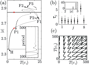
Figure 4: Dynamical features of six-node network motif from fig. 3 of Mackey-Glass systems (12). (a): Bifurcation diagram for $T\left(c_{1}\right)\in\left[0,23\right]$ and fixed $T\left(c_{2}\right)=10$, $T\left(c_{3}\right)=7$. Black lines correspond to stable solutions and gray to unstable. Solid branches are equilibria, dashed are periodic solutions. Bifurcations are denoted by ’H’ (Hopf), ’P[$n$]’ (period doubling), and ’F[$n$]’ (fold). The ordinate measures the norm $|x|$ and the inset shows the period along the main branch. Red crosses indicate the observed solutions from chart (b). (b): 50 random realizations of single delays which keep constant $T\left(c_{1}\right)=5$, $T\left(c_{2}\right)=10$, and $T\left(c_{3}\right)=7$. Each dot corresponds to a realization of $\tau_{j}$. Mean and standard deviation are indicated by squares and bars. For each choice of delays, constant initial functions were drawn from a uniform distribution on $\left[0,1.5\right]$. The inset bars indicate the number of observed solutions $\boldsymbol{x}\left(t\right)$, $t\in[10^{5},1.1\times 10^{5}]$, with the norm $|\boldsymbol{x}|$ in their base interval. Chart (c) shows the trace and reappearances of the Hopf bifurcations in the $T\left(c_{1}\right)$-$T\left(c_{2}\right)$-plane.

4 Summary and discussion

We have presented a universal tool for the reduction of discrete interaction-delays in networks of dynamical systems. It allows to simplify the coupling structure without any loss of information. We have shown that the number of essential delays which determine the dynamics equals the cycle space dimension of the network, and that systems whose roundtrip times along the fundamental semicycles coincide are dynamically equivalent. Even if the roundtrip times are given, the distribution of the delays which yields them is not unique. This provides the opportunity to choose a delay distribution that is best suitable for the problem under consideration. In some cases, as for instance for a unidirectional ring of identical systems with inhomogeneous delays, the right choice of timeshifts allows to uncover hidden symmetries and thereby to simplify the analysis of the system considerably [41, 31]. Conversely, the same transformation was applied to design pattern generators [19, 18] starting from the system with homogeneous delays. Our results are an important step towards the systematization and classification of dynamics on networks with multiple delays. As a main consequence for general coupling structures, the bifurcation analysis can be simplified to a great extent as we have shown in the example of coupled Mackey-Glass systems. The benefits of the reduction seem to be the highest for networks with sparse connectivity. Nevertheless, in highly connected networks, reductions of delays along selected links (e.g. the ones with highest connection weight) or in separate motifs can be a useful application. Furthermore, it seems a promising endeavor to study the potential of the delay transformation to speed up numerical procedures. We have observed that the time it takes to integrate numerically two equivalent systems may vary extremely depending on the distribution of the individual delays. Finally, the results which were presented in this paper can be extended straightforwardly to many other types of local dynamics like time-discrete systems or evolution equations.

Acknowledgments

We thank M. Zaks for useful discussions and the DFG for financial support in the framework of the Collaborative Research Center (SFB) 910 and the International Research Trainig Group (IRTG) 1740.

References

- [1] Tal Danino, Octavio Mondragon-Palomino, Lev Tsimring, and Jeff Hasty. A synchronized quorum of genetic clocks. Nature, 463:326–330, 2010.
- [2] Volkan Sevim, Xinwei Gong, and Joshua E. S. Socolar. Reliability of transcriptional cycles and the yeast cell-cycle oscillator. PLoS Comput Biol, 6(7):e1000842, 07 2010.
- [3] Erin L. O’Brien, Elizabeth Van Itallie, and Matthew R. Bennett. Modeling synthetic gene oscillators. Mathematical Biosciences, 236(1):1 – 15, 2012.
- [4] Jiaxu Li and Yang Kuang. Analysis of a model of the glucose-insulin regulatory system with two delays. SIAM Journal on Applied Mathematics, 67(3):757–776, 2007.
- [5] Uwe an der Heiden. Delays in physiological systems. Journal of mathematical biology, 8(4):345–364, 1979.
- [6] M. C. Mackey and L. Glass. Oscillation and chaos in physiological control systems. Science, 197:287, 1977.
- [7] Yang Kuang. Delay Differential Equations with Applications in Population Dynamics, volume 191 of Mathematics in science and engineering. Academic Press, 1993.
- [8] Miguel C. Soriano, Jordi García-Ojalvo, Claudio R. Mirasso, and Ingo Fischer. Complex photonics: Dynamics and applications of delay-coupled semiconductors lasers. Rev. Mod. Phys., 85:421–470, Mar 2013.
- [9] O. D’Huys, R. Vicente, T. Erneux, J. Danckaert, and I. Fischer. Synchronization properties of network motifs: Influence of coupling delay and symmetry. Chaos, 18(3):037116, 2008.
- [10] Anthony L. Franz, Rajarshi Roy, Leah B. Shaw, and Ira B. Schwartz. Effect of multiple time delays on intensity fluctuation dynamics in fiber ring lasers. Phys. Rev. E, 78(1):016208, 2008.
- [11] Micha Nixon, Moti Fridman, Eitan Ronen, Asher A. Friesem, Nir Davidson, and Ido Kanter. Controlling synchronization in large laser networks. Phys. Rev. Lett., 108:214101, May 2012.
- [12] C. Leibold and J. L. van Hemmen. Spiking neurons learning phase delays: How mammals may develop auditory time-difference sensitivity. Phys. Rev. Lett., 94(16):168102, April 2005.
- [13] Enrico Rossoni, Yonghong Chen, Mingzhou Ding, and Jianfeng Feng. Stability of synchronous oscillations in a system of hodgkin-huxley neurons with delayed diffusive and pulsed coupling. Phys. Rev. E, 71, 2005.
- [14] R. M. Memmesheimer and M. Timme. Designing complex networks. Physica D, 224(1-2):182–201, December 2006.
- [15] Tae-Wook Ko and G. Bard Ermentrout. Effects of axonal time delay on synchronization and wave formation in sparsely coupled neuronal oscillators. Physical Review E (Statistical, Nonlinear, and Soft Matter Physics), 76(5):056206, 2007.
- [16] Douglas J. Bakkum, Zenas C. Chao, and Steve M. Potter. Long-term activity-dependent plasticity of action potential propagation delay and amplitude in cortical networks. PLoS ONE, 3(5):e2088, 05 2008.
- [17] Sue Ann Campbell. Time delays in neural systems. In Handbook of brain connectivity, pages 65–90. Springer, 2007.
- [18] S. Yanchuk, P. Perlikowski, O. V. Popovych, and P. A. Tass. Variability of spatio-temporal patterns in non-homogeneous rings of spiking neurons. Chaos, 21:047511, 2011.
- [19] Oleksandr V. Popovych, Serhiy Yanchuk, and Peter A. Tass. Delay- and coupling-induced firing patterns in oscillatory neural loops. Phys. Rev. Lett., 107:228102, 2011.
- [20] C. E. Carr. Processing of temporal information in the brain. Annu. Rev. Neurosci., 16:223–243, 1993.
- [21] HamidReza Noori and Willi Jäger. Neurochemical oscillations in the basal ganglia. Bulletin of Mathematical Biology, 72(1):133–147, 2010.
- [22] John E. Lisman and Anthony A. Grace. The hippocampal-vta loop: Controlling the entry of information into long-term memory. Neuron, 46(5):703 – 713, 2005.
- [23] Thomas Erneux. Applied Delay Differential Equations, volume 3 of Surveys and Tutorials in the Applied Mathematical Sciences. Springer, 2009.
- [24] Jennifer Foss, André Longtin, Boualem Mensour, and John Milton. Multistability and delayed recurrent loops. Phys. Rev. Lett., 76:708–711, 1996.
- [25] G. Giacomelli and A. Politi. Relationship between delayed and spatially extended dynamical systems. Phys. Rev. Lett., 76(15):2686–2689, 1996.
- [26] J. K. Hale and S. M. Tanaka. Square and pulse waves with two delays. Journal of Dynamics of Differential Equations, 12:1–30, 2000.
- [27] V. Flunkert, S. Yanchuk, T. Dahms, and E. Schöll. Synchronizing distant nodes: A universal classification of networks. Phys. Rev. Lett., 105(25):254101, 2010.
- [28] Sven Heiligenthal, Thomas Dahms, Serhiy Yanchuk, Thomas Jüngling, Valentin Flunkert, Ido Kanter, Eckehard Schöll, and Wolfgang Kinzel. Strong and weak chaos in nonlinear networks with time-delayed couplings. Phys. Rev. Lett., 107:234102, 2011.
- [29] I. Kanter, M. Zigzag, A. Englert, F. Geissler, and W. Kinzel. Synchronization of unidirectional time delay chaotic networks and the greatest common divisor. EPL (Europhysics Letters), 93(6):60003, 2011.
- [30] Guy Van der Sande, Miguel C. Soriano, Ingo Fischer, and Claudio R. Mirasso. Dynamics, correlation scaling, and synchronization behavior in rings of delay-coupled oscillators. Physical Review E (Statistical, Nonlinear, and Soft Matter Physics), 77(5):055202, 2008.
- [31] P. Perlikowski, S. Yanchuk, O. V. Popovych, and P. A. Tass. Periodic patterns in a ring of delay-coupled oscillators. Phys. Rev. E, 82(3):036208, Sep 2010.
- [32] Reinhard Diestel. Graph Theory. Springer-Verlag, Heidelberg, 2010.
- [33] D. Terman, J. E. Rubin, A. C. Yew, and C. J. Wilson. Activity Patterns in a Model for the Subthalamopallidal Network of the Basal Ganglia. Journal of Neuroscience, 22(7):2963–2976, 2002.
- [34] Yoshihisa Tachibana, Hirokazu Iwamuro, Hitoshi Kita, Masahiko Takada, and Atsushi Nambu. Subthalamo-pallidal interactions underlying parkinsonian neuronal oscillations in the primate basal ganglia. European Journal of Neuroscience, 34(9):1470–1484, 2011.
- [35] J. K. Hale and S. M. Verduyn Lunel. Introduction to Functional Differential Equations. Springer-Verlag, 1993.
- [36] Leonhard Lücken, Jan Philipp Pade, Kolja Knauer, and Serhiy Yanchuk. Parameter space dimension for networks with transmission delays. arXiv:1301.2051, January 2013.
- [37] L. Appeltant, M. C. Soriano, G. Van der Sande, J. Danckaert, S. Massar, J. Dambre, B. Schrauwen, C. R. Mirasso, and I. Fischer. Information processing using a single dynamical node as complex system. Nature Comm, 2, 2011.
- [38] Miguel C. Soriano, Guy Van der Sande, Ingo Fischer, and Claudio R. Mirasso. Synchronization in simple network motifs with negligible correlation and mutual information measures. Phys. Rev. Lett., 108:134101, Mar 2012.
- [39] K. Engelborghs, T. Luzyanina, and D. Roose. Numerical bifurcation analysis of delay differential equations using dde-biftool. ACM Trans. Math. Software, 28(1):1–21, 2002.
- [40] Paul Glendinning and Colin Sparrow. Local and global behavior near homoclinic orbits. Journal of Statistical Physics, 35:645–696, 1984.
- [41] P. Baldi and A. Atia. How delays affect neural dynamics and learning. IEEE Transactions on Neural Networks, 5:1045–9227, 1994.