On the local nature and scaling of chaos in weakly nonlinear disordered chains

Abstract

The dynamics of a disordered nonlinear chain can be either regular or chaotic with a certain probability. The chaotic behavior is often associated with the destruction of Anderson localization by the nonlinearity. In the present work, it is argued that at weak nonlinearity chaos is nucleated locally on rare resonant segments of the chain. Based on this picture, the probability of chaos is evaluated analytically. The same probability is also evaluated by direct numerical sampling of disorder realizations, and quantitative agreement between the two results is found.

I Introduction

Dynamics of classical disordered nonlinear chains is governed by an interplay of two fundamental phenomena: Anderson localization (AL) and chaos. AL, originally introduced as full suppression of diffusion by interference in random lattices Anderson1958 and used to explain electronic metal-insulator transitions, turned out to be a universal wave phenomenon and was observed in such diverse systems as microwaves, light, acoustic waves, and ultracold atoms Lagendijk2009 . It is most pronounced in one dimension, where all eigenmodes of a disordered linear system are exponentially localized by arbitrarily weak disorder Gertsenshtein1959 .

By now, AL is well understood for linear systems Evers2008 . In the presence of a nonlinearity, the situation is more complicated, and many fundamental questions are still open. For example, it is unclear what happens to an initially localized wave packet at very long times (see Ref. Fishman2012 for a review). In a linear system with AL, it remains exponentially localized at all times. With nonlinearity, the wave packet width was found to increase as a subdiffusive power of time $t$ in numerical simulations Shepelyansky1993 ; Pikovsky2008 ; Flach2009 ; Bodyfelt2011 . In contrast, a rigorous argument shows that at long times the spreading, if any, must be slower than any power of time Wang2009 . Analysis of perturbation theory in the nonlinearity suggests that there is a front propagating as $~{}\ln{t}$ beyond which the wave packet is localized exponentially Fishman2009 . An indication for a slowing down of the power law has also been seen in the scaling analysis of numerical results Mulansky2011 . Finally, a possible mechanism of breakdown of subdiffusion at long times is presented in Ref. Michaely2012 .

One of the difficulties in describing nonlinear system is that their dynamics can be chaotic Chirikov1979 ; Zaslavsky ; Lichtenberg . For Hamiltonian systems, close to integrable and with a finite number of the degrees of freedom, the volume of the chaotic phase space is small as long as the integrability-breaking perturbation (in our case, the coupling between the oscillators or the nonlinearity) is weak, as guaranteed by the Kolmogorov-Arnol’d-Moser (KAM) theorem.

For a random system, the description of chaotic and regular motion has to be probabilistic. In the pioneering work Frohlich1986 , the existence of a dense set of regular trajectories was proven for a class of disordered weakly-nonlinear lattices. It has been argued for the disordered nonlinear Schrödinger chain (DNLS) that the measure of such set in the phase space is finite Johansson2010 . This measure, averaged over the disorder, was recently estimated for DNLS both analytically Basko2011 and numerically Pikovsky2011 . In particular, when the nonlinearity is weak, chaos should appear locally. Namely, for a sufficiently long chain, arbitrarily separated in two segments, the probability to be on a regular trajectory is given by the product of the two individual probabilities for the segments. This naturally follows from two conditions: (i) if any of the segments is chaotic, the whole chain is chaotic, and (ii) the probabilities for the two segments are independent. Moreover, in Ref. Basko2011 an explicit mechanism for chaos generation was proposed: two coinciding resonances for rare combinations of three oscillators. Still, the results of Refs. Basko2011 ; Pikovsky2011 , did not agree quantitatively, and the origin of the discrepancy is currently not understood. Evidence for a local origin of chaos has also been found in the simulations of the dynamics of a classical spin chain Pal2009 .

In the present work, the probability of chaotic behavior (appearance of a non-zero Lyapunov exponent) is studied for another system of coupled nonlinear oscillators [see Eq. (LABEL:HFSW=) below], which turns out to be simpler to analyze than the DNLS. The probability of chaos is calculated at low energy densities $\epsilon$ by two different methods: (i) by the analysis of the phase space of an effective Hamiltonian describing a resonant triple of oscillators, in the spirit of Ref. Basko2011 , and (ii) by direct numerical sampling of many disorder realizations, and counting those with nonzero Lyapunov exponent, analogously to Ref. Pikovsky2011 .

Our main results are the following. (i) The two calculations agree quantitatively, including both the leading low-$\epsilon$ scaling exponent, and the numerical prefactor, thereby confirming the dominant role of resonant triples in generation of chaos at low energies. (ii) This agreement sets in at unexpectedly small values of $\epsilon$, while at moderately low $\epsilon$ the numerical results fall on an intermediate asymptotics. This intermediate asymptotics is not controlled by any small parameter and seems to exist for purely numerical reasons; the microscopic mechanism responsible for it remains unclear at the moment.

II Statement of the problem

Here we study the model defined by the Hamiltonian

$$\begin{split}&H(\{p_{n},q_{n}\})={H}_{0}(\{p_{n},q_{n}\})+H_{\mathrm{int}}(\{p_{n},q_{n}\})=\\ &=\sum_{n=1}^{L}\left(\frac{p_{n}^{2}}{2m}+\frac{m\omega_{n}^{2}q_{n}^{2}}{2}\right)+\frac{g}{4}\sum_{n=1}^{L-1}\left(q_{n+1}-q_{n}\right)^{4},\end{split}$$ (1)

where $q_{n},p_{n}$ are the coordinate and momentum of the $n$th oscillator, and $\omega_{n}^{2}$ are independent random variables uniformly distributed in the interval

$$\frac{W^{2}}{2}<\omega_{n}^{2}<\frac{3W^{2}}{2},$$ (2)

$W$ being the disorder strength. This model belongs to the class of models considered in Ref. Frohlich1986 . It has also been studied in Refs. Mulansky2011 ; Ivanchenko2011 , however, in the latter two works focused on spreading of an initially localized wave packet, rather than on the probability of chaos.

The model of Eq. (LABEL:HFSW=) is different from DNLS in two aspects. First, it has only one conserved quantity (energy) in contrast to the two (energy and total norm) for DNLS. Second, it has only one dimensionless parameter,

$$\epsilon_{n}=\frac{g}{m^{2}W^{4}}\left(\frac{p_{n}^{2}}{2m}+\frac{m\omega_{n}^{2}q_{n}^{2}}{2}\right),$$ (3)

controlling both the nonlinearity and the coupling between the oscillators. In DNLS they are controlled separately by two independent dimensionless parameters, and when both are small, it matters which one is smaller. In the FSW case, both limits of weak coupling and weak nonlinearity correspond to $\epsilon_{n}\to{0}$, which makes it easier to analyze than DNLS. From now on, we measure momenta, coordinates, and time in the units of $\sqrt{m^{3}W^{4}/g}$, $\sqrt{mW^{2}/g}$, and $1/W$, respectively, which is equivalent to setting $m,W,g=1$.

For a given realization of disorder $\{\omega_{n}^{2}\}$ and a given initial condition $\{p_{n},q_{n}\}$, the system trajectory is either regular (quasi-periodic) or chaotic. Characterizing each initial condition by the typical energy $\epsilon$ per oscillator, we define the probability for the initial condition to be chaotic as

$$\begin{split}{P}(\epsilon,L)={}&{}\int\Theta(\{p_{n},q_{n}\},\{\omega_{n}^{2}\})\times\\ {}&{}\times\prod_{n=1}^{L}\delta\!\left(\frac{p_{n}^{2}+\omega_{n}^{2}q_{n}^{2}}{2}-\epsilon\right)\frac{dp_{n}dq_{n}}{2\pi/\omega_{n}}\,d\omega_{n}^{2},\end{split}$$ (4)

where $\Theta(\{p_{n},q_{n}\},\{\omega_{n}^{2}\})=1$ if the trajectory is chaotic and zero otherwise. Eq. (4) corresponds to fixing the energies of all oscillators to be $\epsilon$, and will be referred to as the fixed-$\epsilon$ ensemble. Alternatively, one can fix the energies only on average, replacing the $\delta$-function in Eq. (4) by $(1/\epsilon)\exp[-(p_{n}^{2}+\omega_{n}^{2}q_{n}^{2})/(2\epsilon)]$, i. e. a thermal distribution with temperature $\epsilon$ (provided that $\epsilon\ll{1}$, which is our main focus) Eperosc . In the present paper we will work with the fixed-$\epsilon$ ensemble which is easier to handle numerically. The corresponding initial conditions can be represented as

$$p_{n}=\sqrt{2\epsilon}\cos\phi_{n},\quad q_{n}=\frac{\sqrt{2\epsilon}}{\omega_{n}}\sin\phi_{n},$$ (5)

where the phases $\phi_{n}$ are uniformly distributed on the interval $[0,2\pi]$.

The property of locality, mentioned in the introduction, leads to the dependence ${P}(\epsilon,L)=1-e^{-w(\epsilon)\,L}$ at sufficiently large $L$, where the quantity $w(\epsilon)$, which we call average chaotic fraction (as in Ref. Basko2011 ), does not depend on $L$. The main goal of the present work is to establish its asymptotic behavior $w(\epsilon\to{0})$, by two methods: (i) relating it to the chaotic phase volume of three resonant oscillators, as in Ref. Basko2011 , and (ii) by direct numerical sampling, analogously to Ref. Pikovsky2011 . The latter method also provides a check for the locality hypothesis: if indeed ${P}(\epsilon,L)=1-e^{-w(\epsilon)\,L}$, the quantity

$$\frac{1}{L}\ln\frac{1}{1-{P}(\epsilon,L)}$$

does not depend on $L$, so that all curves for different $L$ should collapse on a single curve $w(\epsilon)$. Thanks to the relative simplicity of the system defined by Eq. (LABEL:HFSW=), both calculations can be carried out all the way to the final result, which turns out to be

$$w(\epsilon\to{0})=A\epsilon^{2},$$ (6)

where $A\approx{1}.37\cdot{10}^{3}$ for the fixed-$\epsilon$ ensemble.

III Calculation

The reduction of the problem to a few-oscillator configuration Basko2011 is based on the two-resonance picture for weakly non-integrable systems Chirikov1979 ; Zaslavsky ; Lichtenberg . The strongest resonant term in the non-integrable perturbation of an integrable system (the so-called guiding resonance) produces a separatrix in the system phase space. This separatrix is destroyed by another term in the perturbation, which creates a thin stochastic layer in the surrounding part of the phase space. In a disordered system, the main contribution to the chaotic phase space comes from those configurations of disorder and from those regions of the phase space where both perturbation terms are resonant, so one cannot really distinguish between the one responsible for the appearance of the separatrix and the one responsible for its destruction. It is crucial that two resonance conditions should be met simultaneously.

Resonances involving many oscillators are expected to give a subleading contribution to the chaotic phase volume, as the corresponding perturbation terms can be generated in high orders of perturbation theory, thus resulting in high powers of $\epsilon$. The minimal number of oscillators needed to generate chaos in the model of Eq. (LABEL:HFSW=) is two chaosDNLS . However, even if $\omega_{1}\approx\omega_{2}$, the frequency of the separatrix-destroying perturbation, $\omega_{1}+\omega_{2}$, cannot be small for the chosen disorder distribution, $1/2<\omega_{n}^{2}<3/2$, which leads to an exponential suppression of the chaotic phase volume Chirikov1979 ; Zaslavsky ; Lichtenberg . In fact, for the particular case of Eq. (LABEL:HFSW=), the situation is even worse: no separatrix exists in the phase space of the slow motion (see Appendix A.1). Thus, the dominant contribution to the chaotic phase volume should come from triples of oscillators with all three frequencies close to each other. The oscillators should also be neighboring each other in space, since coupling distant oscillators requires high orders of perturbation theory and results in a high power of $\epsilon$. Thus, $w(\epsilon)$ is essentially determined by the probability (per unit length along the chain) to find three neighboring oscillators whose frequencies differ by $\sim\epsilon$. This fixes the power $w(\epsilon)\propto\epsilon^{2}$.

To put this argument on a quantitative basis, we assume $\omega_{1}\approx\omega_{2}\approx\omega_{3}$, and average Eq. (LABEL:HFSW=) over fast oscillations (see Appendix A.2 for details). This gives the effective Hamiltonian of the resonant triple:

$$\begin{split}H_{\mathrm{tr}}={}&{}\Omega|\Psi_{1}|^{2}-(\Omega+\Omega^{\prime})|\Psi_{2}|^{2}+\Omega^{\prime}|\Psi_{3}|^{2}+\\ {}&{}+\frac{1}{2}\left(|\Psi_{1}|^{4}+|\Psi_{3}|^{4}+|\Psi_{1}-\Psi_{2}|^{4}+|\Psi_{2}-\Psi_{3}|^{4}\right),\end{split}$$ (7)

written in terms of complex canonical variables $i\Psi_{n}^{*},\Psi_{n}$, related to $p_{n},q_{n}$ as

$$\Psi_{n}=\frac{e^{i\bar{\omega}{t}}}{\sqrt{I}}\left(\frac{p_{n}}{\sqrt{2\omega_{n}}}-i\sqrt{2\omega_{n}}q_{n}\right),\quad I=\sum_{n=1}^{3}\frac{p_{n}^{2}+\omega_{n}^{2}q_{n}^{2}}{2\omega_{n}}.$$ (8)

where $\bar{\omega}=(\omega_{1}+\omega_{2}+\omega_{3})/3$. The rescaling of $\Psi$’s by $\sqrt{I}$ restricts them to the unit sphere, $|\Psi_{1}|^{2}+|\Psi_{2}|^{2}+|\Psi_{3}|^{2}=1$, which is invariant under the dynamics generated by the Hamiltonian in Eq. (7). The rescaled frequency mismatches $\Omega,\Omega^{\prime}$ are defined as

$$\Omega=\frac{2\omega_{1}-\omega_{2}-\omega_{3}}{(9/4)(I/\bar{\omega}^{2})},\quad\Omega^{\prime}=\frac{2\omega_{3}-\omega_{2}-\omega_{1}}{(9/4)(I/\bar{\omega}^{2})},$$ (9)

For the fixed-$\epsilon$ ensemble, Eq. (4), we have $I=3\epsilon/\bar{\omega}+O(\epsilon^{2})$, and the initial condition should be chosen in the form $\Psi_{1}=e^{-i\varphi}/\sqrt{3}$, $\Psi_{2}=e^{i\varphi+i\varphi^{\prime}}/\sqrt{3}$ $\Psi_{3}=e^{-i\varphi^{\prime}}/\sqrt{3}$, where $0<\varphi,\varphi^{\prime}<2\pi$ are random phases (the global phase drops out of the result). Then, defining $\Theta(\varphi,\varphi^{\prime};\Omega,\Omega^{\prime})$ to be 1 if the corresponding trajectory is chaotic for given values of $\varphi,\varphi^{\prime},\Omega,\Omega^{\prime}$ and 0 otherwise, we obtain from Eq. (4):

$$w(\epsilon)=81\epsilon^{2}\int\limits_{-\infty}^{\infty}d\Omega\,d\Omega^{\prime}\int\limits_{0}^{2\pi}\frac{d\varphi}{2\pi}\frac{d\varphi^{\prime}}{2\pi}\,\Theta(\varphi,\varphi^{\prime};\Omega,\Omega^{\prime}).$$ (10)

Since neither the Hamiltonian [Eq. (7)] nor the initial condition contain any small parameters, the integral over $\Omega,\Omega^{\prime}$ in Eq. (10) is dominated by $|\Omega|,|\Omega^{\prime}|\sim{1}$, while for larger mismatches the chaotic regions quickly shrink. Thus, the limits of the $\Omega,\Omega^{\prime}$-integration (which are $\sim{1}/\epsilon$) have been extented to infinity. The factor $\epsilon^{2}$ in front of the integral appears because $\Omega,\Omega^{\prime}\propto{1}/I\propto{1}/\epsilon$, see Eq. (9). The integral is evaluated numerically to be $16.9\pm{0.2}$, leading to $w(\epsilon\to{0})=A\epsilon^{2}$ with $A=1.37\cdot{10}^{3}$, as stated in Eq. (6).

The key element of the numerical procedure is the criterion which enables one to distinguish between regular and chaotic motion. Formally, one studies the largest Lyapunov exponent $\sigma$, characterizing the mean exponential rate of divergence of two initially close trajectories,

$$\sigma=\lim\limits_{t\to\infty}\frac{\Lambda(t)}{t},\quad\Lambda(t)=\ln\frac{d(t)}{d(0)},$$ (11)

where $d(t)$ is the distance between points belonging to the two trajectories Lichtenberg . If $\sigma=0$, the motion is regular, if $\sigma>0$, it is chaotic. In practice, one may integrate the equations of motion for a sufficiently long time $T$, and consider $\sigma=0$ if $\Lambda(T)/T<(\mbox{a few times})(1/T)$ Pikovsky2011 ; Mulansky2011a . Here we use a slightly different criterion, based on the behavior of $\Lambda(t)$ in the whole integration interval $0<t<T$. Namely, we check how well $\Lambda(t)$ can be approximated by a logarithmic function, as described in Appendix B.

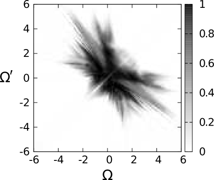
Figure 1: A grayscale plot of the integral $\int_{0}^{2\pi}(d\varphi/2\pi)(d\varphi^{\prime}/2\pi)\,\Theta(\varphi,\varphi^{\prime};\Omega,\Omega^{\prime})$ as a function of $\Omega,\Omega^{\prime}$.

In Fig. 1, the $\varphi,\varphi^{\prime}$-integral in Eq. (10) is plotted as a function of $\Omega,\Omega^{\prime}$. The fact that the chaotic region is confined in all directions, represents a numerical proof of the statement that chaos arises mostly in the regions where two resonant conditions are satisfied simultaneously.

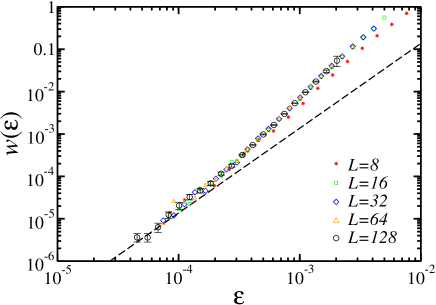
Figure 2: (color online) $(1/L)|\ln(1-{P}_{L}(\epsilon))|$ versus $\epsilon$ for the fixed-density excitation and different values of $L=8,16,32,64,128$ (symbols). The error bars for $L=128$ correspond to the relative error $1/\sqrt{N}$, where $N$ is the absolute number of detected events. The dashed line represents the dependence $w(\epsilon)=(1.37\cdot{10}^{3})\,\epsilon^{2}$, obtained from the resonant-triple calculation.

Using the same algorithm, $w(\epsilon)$ was also calculated by direct numerical sampling of disorder realizations on chains of lengths $L=8,16,32,64,128$. For $\epsilon>{10}^{-4}$, the integration time $T=10^{6}$ and averaging over $10^{4}$ realizations was performed for each $L$; for smaller $\epsilon<10^{-4}$, when the probability ${P}_{L}(\epsilon)$ is also very small, more than $4\cdot{10}^{4}$ realizations were required to accumulate at least $N=20$ events for each data point. Then $1/\sqrt{N}$ was assumed to give the relative uncertainty of the obtained value $w(\epsilon)$. Also, for $\epsilon<10^{-4}$, the integration time had to be increased to $T=3\cdot{10}^{6}$ in order to reliably distinguish between regular and chaotic dynamics (see also Appendix B).

The numerical results, as well as the dependence $w(\epsilon)=(1.37\cdot{10}^{3})\,\epsilon^{2}$, obtained from Eq. (10), are shown in Fig. 2 by the symbols and the dashed line, respectively. Fig. 2 represents the main result of the present work. Starting from $L=16$, the collapse of the numerical data is very good, which numerically proves the local origin of chaos. At $\epsilon<3\cdot{10}^{-4}$ the numerical data fall on the dashed line. At larger $\epsilon$ the data collapses on some intermediate asymptotics for $w(\epsilon)$, which can be approximated by a power law $w(\epsilon)=B\epsilon^{\beta}$ with the exponent $\beta=2.85\pm{0}.1$ and a surprisingly large prefactor $B=(1-5)\cdot{10}^{6}$. The precise mechanism responsible for this intermediate asymptotics is not clear at the moment. This mechanism is likely to involve a larger number of oscillators (more than three), since (i) it is in this region of $\epsilon$ that the symbols for short chains ($L=8$) exhibit a systematic deviation from those for long chains in Fig. 2, in the direction of suppression of the intermediate asymptotics; (ii) for a single-site initial excitation (see Fig. 3 below) the intermediate asymptotics is completely absent, indicating that it requires a certain initial spread.

IV Relation to wave packet spreading

In this context, one should mention the result reported in Ref. Ivanchenko2011 , where the probability of subdiffusive spreading of an initially localized wave packet was studied for exactly the same model, Eq. (LABEL:HFSW=). Namely, it was argued that an initially localized wave packet either stays localized forever or spreads indefinitely, and the probability of spreading was estimated to be proportional to $\epsilon$ at small $\epsilon$. In the present work, the probability of chaos, was shown to scale as $\epsilon^{2}$. Since the latter is smaller than the former, the combination of the two results would suggest that the wave packet spreading does not require chaos, which is quite counter-intuitive. However, in the author’s opinion, it is more plausible that the probability of spreading was strongly overestimated in Ref. Ivanchenko2011 , as discussed below.

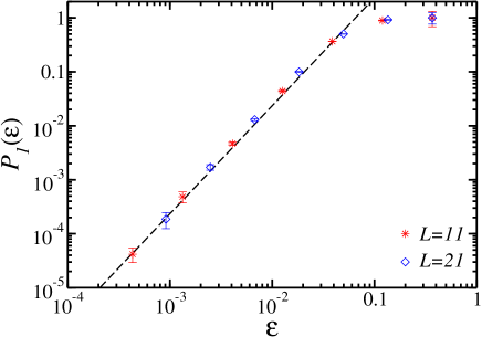
Figure 3: (color online) The probability of chaos versus $\epsilon$ for a single-site excitation and two values of $L=11,21$ (symbols). The dashed line represents the dependence $235\,\epsilon^{2}$, obtained from the resonant-triple calculation of Appendix C.

First, let us exclude the trivial possibility that the difference between the two results is simply due to the fact that initial conditions studied in Ref. Ivanchenko2011 correspond to excitation localized on a single site, while a finite density was assumed in the present work. Indeed, for a finite density the trajectory is chaotic when a resonant triple occurs anywhere on the chain, while for a single-site excitation the condition is simply that the resonant triple includes the excited site. This affects the scaling with $L$, but not with $\epsilon$: the probability of chaos for a single-site excitation scales as $P_{1}(\epsilon)=A_{1}\epsilon^{2}$ and is independent of $L$. The resonant-triple calculation gives $A_{1}\approx{235}$ (see Appendix C), which is also confirmed by the direct numerical sampling, as shown in Fig. 3. (Note also the direct crossover from 1 to $A_{1}\epsilon^{2}$ without any intermediate asymptotics).

The analytical arguments of Ref. Ivanchenko2011 are based on the assumption that a single resonance is sufficient for spreading. This immediately gives the probability scaling $\propto\epsilon$. However, it is not clear why a single resonance should lead to unlimited spreading; indeed, an isolated nonlinear resonance is known to produce just periodic oscillations Chirikov1979 ; Zaslavsky .

The numerical procedure of Ref. Ivanchenko2011 was based on the study of the participation number,

$$\mathcal{P}=\left(\sum_{n=1}^{L}E_{n}\right)^{2}\left(\sum_{n=1}^{L}E_{n}^{2}\right)^{-1},$$ (12)

where the on-site energy corresponding to the model of Eq. (LABEL:HFSW=) can be defined as

$$E_{n}=\frac{p_{n}^{2}}{2m}+\frac{m\omega_{n}^{2}q_{n}^{2}}{2}+\frac{g}{8}\left[(q_{n}-q_{n-1})^{4}+(q_{n}-q_{n+1})^{4}\right],$$ (13)

for all $n$ except $n=1$ and $n=L$, where only one nonlinear term corresponding to the unique neighbor should be taken. For a perfectly thermalized chain $\mathcal{P}=L/2$, and for a state perfectly localized on a single site $\mathcal{P}=1$. In Ref. Ivanchenko2011 , a trajectory was counted as spreading if $\mathcal{P}$ exceeded an arbitrarily chosen threshold of 1.2 by the time $t=10^{9}$. Thus, the main assumption behind the numerics was that if a trajectory has overcome the limit $\mathcal{P}=1.2$ at $t=10^{9}$, it will spread forever. In the following, it is argued that this is unlikely to be true for the majority of the trajectories.

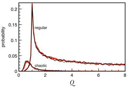
Figure 4: (color online) Partial contributions to the probability distribution of $\mathcal{Q}=1/(\mathcal{P}-1)$ [see Eq. (12)] from regular and chaotic trajectories (upper and lower curves, respectively) at times $t=10^{5},10^{6}$ [thick red (gray) and thin black curves, respectively] for two chain lengths $L=11,21$ (dotted and solid curves, respectively) for $\epsilon=0.01$.

Let us analyze the probability distribution of $\mathcal{Q}=1/(\mathcal{P}-1)$, which is a more convenient quantity to analyze at small $\epsilon$, when the spreading trajectories correspond to $\mathcal{Q}\sim{1}$, while the overwhelming majority of strongly localized solutions form the broad large-$\mathcal{Q}$ tail. In Fig. 4 we separately plot the two contributions to the distribution of $\mathcal{Q}$ from regular and chaotic trajectories at $t=10^{5},10^{6}$ for $L=11,21$. The value of $\epsilon=0.01$ is sufficiently small to be in the asymptotic regime, as seen from Fig. 3, and more than 50000 disorder realizations were used for each of the four pairs of curves. The difference between $L=11$ and $L=21$ curves is not detectable within the numerical resolution, while a slight difference between $t=10^{5}$ and $t=10^{6}$ curves can be seen on the low-$\mathcal{Q}$ side of the chaotic curves, which indicates some spreading of the wave packet. The fact that a large part of the probability distribution at $\mathcal{Q}<5$ (corresponding to $\mathcal{P}>1.2$) belongs to the large-$\mathcal{Q}$ tail due to localized trajectories, suggests that many trajectories counted as spreading in Ref. Ivanchenko2011 , in fact were not.

Another argument, not relying on numerical integration over long times, can be given by considering a regular solution, predominantly localized on site $n$. The amplitude on the neighboring sites $n-1,n+1$ can be found by perturbation theory,

$$q_{n}=\frac{\sqrt{2\epsilon}}{\omega_{n}}\,\cos\omega_{n}t+O(\epsilon^{3/2}),$$ (14a)

$$q_{n\pm{1}}=\frac{\epsilon^{3/2}}{\sqrt{2}\omega_{n}^{3}}\left(\frac{3\cos\omega_{n}t}{\omega_{n\pm{1}}^{2}-\omega_{n}^{2}}+\frac{\cos{3}\omega_{n}t}{\omega_{n\pm{1}}^{2}-9\omega_{n}^{2}}\right)+O(\epsilon^{5/2}),$$

which gives the participation number

$$\begin{split}\mathcal{P}\approx{}&{}{1}+2\,\frac{\epsilon_{n-1}+\epsilon_{n+1}}{\epsilon_{n}}\approx\\ \approx{}&{}1+\frac{9\epsilon^{2}}{4\omega_{n}^{6}}\sum_{\pm}\left[\frac{\omega_{n\pm{1}}^{2}+\omega_{n}^{2}}{(\omega_{n\pm{1}}^{2}-\omega_{n}^{2})^{2}}+\frac{\omega_{n\pm{1}}^{2}/9+\omega_{n}^{2}}{(\omega_{n\pm{1}}^{2}-9\omega_{n}^{2})^{2}}\right].\end{split}$$ (15)

Here we omitted oscillating terms, which at large $t\gg{1}$ quickly vanish upon disorder averaging), as well as terms which do not contain potentially small denominators and thus are bounded by $O(\epsilon)$ [such as $3\epsilon/(4\omega_{n}^{4})$, originating from the $(q_{n\pm{1}}-q_{n})^{4}$ contribution to $E_{n\pm{1}}$].

From Eq. (15), one can find the probability of $\mathcal{P}>1.2$ at small $\epsilon$ by noting that $\mathcal{P}>1.2$ may occur when either $\omega_{n+1}$ or $\omega_{n-1}$ is close to $\omega_{n}$. The probability of both occurring simultaneously can be neglected, as well as the probability of $\omega_{n\pm{1}}$ being close to $3\omega_{n}$, as these probabilities are $\propto\epsilon^{2}$. Then, the probability of $\mathcal{P}>1.2$ is given by

$$\begin{split}\mathop{\mathrm{Pr}}\left\{\mathcal{P}>1.2\right\}\approx{}&{}\sum_{\pm}\mathop{\mathrm{Pr}}\left\{\frac{9\epsilon^{2}}{4\omega_{n}^{6}}\,\frac{\omega_{n\pm{1}}^{2}+\omega_{n}^{2}}{(\omega_{n\pm{1}}^{2}-\omega_{n}^{2})^{2}}>0.2\right\}\approx\\ \approx{}&{}2\mathop{\mathrm{Pr}}\left\{|\omega_{n+1}^{2}-\omega_{n}^{2}|<\frac{1}{\sqrt{0.2}}\,\frac{3\epsilon}{\sqrt{2}\omega_{n}^{2}}\right\}\approx\\ \approx{}&{}\frac{3\sqrt{8}\,\epsilon}{\sqrt{0.2}}\int\limits_{1/2}^{3/2}\frac{d\omega_{n}^{2}}{\omega_{n}^{2}}\approx{20}.8\,\epsilon.\end{split}$$ (16)

The coefficient in front of $\epsilon$ is very close to that obtained numerically for the probability of spreading (see inset of Fig. 3 of Ref. Ivanchenko2011 ).

The fact that Eq. (16), derived under the assumption of validity of perturbation theory at arbitrarily long times (i. e., that the trajectory is localized), gives practically the same result as the numerics of Ref. Ivanchenko2011 , means that almost all trajectories counted as spreading in Ref. Ivanchenko2011 , were in fact localized. Thus, the question of whether the probability of unlimited wave packet spreading scales as $\propto\epsilon$, or $\propto\epsilon^{2}$, or is identically zero, remains open.

V Conclusions

In this work, the probability for a long chain of oscillators, defined by its Hamiltonian, Eq. (LABEL:HFSW=), to be on a chaotic trajectory, was calculated by analyzing the chaotic phase space of rare resonant configurations of three oscillators. The result, $1-e^{-A\epsilon^{2}L}$, agrees with the direct numerical evaluation of Lyapunov exponents for many disorder realizations and initial conditions at sufficiently small values of $\epsilon$, the energy per oscillator. While the coefficient $A$ depends on the specific ensemble used for the initial conditions, the power law $\epsilon^{2}$ is determined by the mere fact that chaotic phase volume is dominated by the regions of the phase space where two resonant conditions for three neighboring oscillators are satisfied simultaneously. This fact was numerically verified for the three-oscillator configuration, see Fig. 1.

The following main conclusions can be drawn from the results of present work. (i) The local nature of chaos, established earlier for the discrete nonlinear Schrödinger equation with disorder (DNLS) in Refs. Basko2011 ; Pikovsky2011 for weak nonlinearity, is further confirmed here for a different model. Namely, the probability of regular dynamics decays with length $L$ as $e^{-wL}$, so $w$ can be called the probability per unit length for the chaos to occur. (ii) Two different ways to calculate this probability, namely, from the analysis of the phase space of a resonant triple, and by direct numerical sampling of disorder realizations, give the same result, but this agreement sets in at unexpectedly small values of $\epsilon\sim{3}\times{10}^{-4}$. At larger $\epsilon$, an intermediate asymptotics is seen in the numerical results. This fact may be relevant for understanding the disagreement between the results of Refs. Basko2011 and Pikovsky2011 for the chaotic probability in the DNLS; indeed, one cannot exclude existence of similar intermediate regimes in DNLS. However, the results of the present work were obtained for a quite different model with a different number of independent parameters, so no quantitative comparison can be made with the DNLS, and the latter should be studied further.

VI Acknowledgements

The author is grateful to M. Ivanchenko, T. Laptyeva, and S. Flach for clarifying discussions of Ref. Ivanchenko2011 , and to S. Fishman for a critical reading of the manuscript.

Appendix A Few-oscillator configurations

It is convenient to pass to the canonical action-angle variables, $(p_{n},q_{n})\to(I_{n},\phi_{n})$:

$$p_{n}=\sqrt{2\omega_{n}I_{n}}\,\cos\phi_{n},\quad q_{n}=\sqrt{\frac{2I_{n}}{\omega_{n}}}\,\sin\phi_{n}.$$ (17)

Hamiltonian (LABEL:HFSW=), averaged over the fast oscillations, (that is, with terms depending on $\phi_{n}+\phi_{n+1}$ omitted) takes the following form:

$$\begin{split}H={}&{}\sum_{n=1}^{L}\omega_{n}I_{n}+\frac{3}{8}\sum_{n=1}^{L-1}\left[\frac{I_{n}}{\omega_{n}}+\frac{I_{n+1}}{\omega_{n+1}}-2\sqrt{\frac{I_{n}I_{n+1}}{\omega_{n}\omega_{n+1}}}\cos(\phi_{n}-\phi_{n+1})\right]^{2}.\end{split}$$ (18)

It should be noted that the part of the Hamiltonian corresponding to two or three oscillators (say, $n,n+1,n+2$) far from the ends of the chain is different from the Hamiltonian given by Eq. (18) for $L=2$ or $L=3$. Indeed, in the former case the Hamiltonian of the $n$th oscillator contains the term $(3/4)I_{n}^{2}/\omega_{n}^{2}$, coming from coupling to the two neighbors $n-1$ and $n+1$, while in the latter case the $n=1$ oscillator has only one neighbor, so the nonlinear term is twice smaller, $(3/8)I_{1}^{2}/\omega_{1}^{2}$.

A.1 Two oscillators

Let $\omega_{n}\approx\omega_{n+1}$ be strongly different from $\omega_{n-1},\omega_{n+2}$. We perform a canonical change of variables of the pair

$$\begin{split}&I=I_{n}+I_{n+1},\quad\phi=\frac{\phi_{n}+\phi_{n+1}}{2},\\ &J=\frac{I_{n}-I_{n+1}}{2},\quad\varphi=\phi_{n}-\phi_{n+1},\end{split}$$ (19)

and further denote $J=(I/2)\cos\vartheta$. Then the Hamiltonian of the pair is given by

$$\begin{split}H={}&{}\frac{\omega_{1}^{\prime}+\omega_{2}^{\prime}}{2}\,I+(\omega_{1}^{\prime}-\omega_{2}^{\prime})(I/2)\cos\vartheta{}+{}\\ {}&{}+\frac{3}{4}\,\frac{I^{2}}{4}\left(\frac{\omega_{1}+\omega_{2}}{\omega_{1}\omega_{2}}-\frac{\omega_{1}-\omega_{2}}{\omega_{1}\omega_{2}}\,\cos\vartheta\right)^{2}{}+{}\\ {}&{}+\frac{3}{2}\,\frac{(I^{2}/4)\sin\vartheta}{(\omega_{1}\omega_{2})^{3/2}}\left[\omega_{1}+\omega_{2}-(\omega_{1}-\omega_{2})\cos\vartheta\right]\cos\varphi{}+{}\\ {}&{}+\frac{3}{4}\,\frac{I^{2}/4}{\omega_{1}\omega_{2}}\,\sin^{2}\vartheta\cos{2}\varphi,\end{split}$$ (20)

where $\omega_{1}^{\prime}=\omega_{n}+4I_{n-1}/(\omega_{n}\omega_{n-1})$, $\omega_{2}^{\prime}=\omega_{n+1}+4I_{n+2}/(\omega_{n+1}\omega_{n+2})$, We can assume $I_{n-1},I_{n+2}$ to be constant, as their changes due to weak non-resonant perturbation are small. This Hamiltonian can be approximately rewritten as

$$H\approx\frac{3}{16}\frac{I^{2}}{\bar{\omega}^{2}}\left(\Omega\cos\vartheta+4\sin\vartheta\cos\varphi+\sin^{2}\vartheta\cos{2}\varphi\right)+$$

$$\qquad\qquad{}+\mathrm{const},$$ (21a)

$$\Omega=\frac{8\bar{\omega}^{2}(\omega_{1}^{\prime}-\omega_{2}^{\prime})}{3I},\quad\bar{\omega}=\frac{\omega_{1}+\omega_{2}}{2}.$$ (21b)

This Hamiltonian has only two elliptic stationary points in the phase space $(\vartheta,\varphi)$ at any value of the rescaled mismatch $\Omega$. Hence, its phase space does not contain a separatrix at all, so we do not expect any chaos at small $\epsilon$.

A.2 Three oscillators

As we are interested in the properties of a resonant triple $n,n+1,n+2$ far from the ends of the chain, let us denote the three frequencies by

$$\begin{split}&\omega^{\prime}_{1}=\omega_{n}+\frac{4I_{n-1}}{\omega_{n}\omega_{n-1}},\\ &\omega^{\prime}_{2}=\omega_{n+1},\\ &\omega^{\prime}_{3}=\omega_{n+2}+\frac{4I_{n+3}}{\omega_{n+2}\omega_{n+3}},\end{split}$$ (22)

and assume $I_{n-1}$ and $I_{n+3}$ to be constant, since their variation is small in the parameter $\epsilon\ll{1}$. Moreover, we can also neglect the modification in the probability distributions of $\omega^{\prime}_{1},\omega^{\prime}_{3}$ with respect to that of $\omega_{n}$, as the difference is again $\sim\epsilon$. The most important contribution to the chaotic fraction will come from the region where the differences $\omega^{\prime}_{1}-\omega^{\prime}_{2}$, $\omega^{\prime}_{2}-\omega^{\prime}_{3}$, are small compared to the frequencies themselves. Having this in mind, let us further denote

$$\bar{\omega}=\frac{\omega^{\prime}_{1}+\omega^{\prime}_{2}+\omega^{\prime}_{3}}{3}.$$ (23)

Introducing the complex canonical coordinates $\psi_{1}=\sqrt{I_{n}}\,e^{-i\phi_{n}}$, $\psi_{2}=\sqrt{I_{n+1}}\,e^{-i\phi_{n+1}}$, $\psi_{3}=\sqrt{I_{n+2}}\,e^{-i\phi_{n+2}}$, whose conjugate momenta are $i\psi_{1}^{*},i\psi_{2}^{*},i\psi_{3}^{*}$, respectively, we can write the Hamiltonian of the triple as

$$\begin{split}H={}&\sum_{i=1}^{3}\omega_{i}^{\prime}\psi_{i}^{*}\psi_{i}+\frac{3}{8}\,\frac{\psi_{1}^{*}\psi_{1}^{*}\psi_{1}\psi_{1}}{(\omega_{1}^{\prime})^{2}}+\frac{3}{8}\,\frac{\psi_{3}^{*}\psi_{3}^{*}\psi_{3}\psi_{3}}{(\omega_{3}^{\prime})^{2}}\\ {}&+\frac{3}{8}\sum_{i=1}^{2}\left(\frac{\psi_{i}^{*}}{\sqrt{\omega_{i}^{\prime}}}-\frac{\psi_{i+1}^{*}}{\sqrt{\omega_{i+1}^{\prime}}}\right)^{2}\left(\frac{\psi_{i}}{\sqrt{\omega_{i}^{\prime}}}-\frac{\psi_{i+1}}{\sqrt{\omega_{i+1}^{\prime}}}\right)^{2}.\end{split}$$ (24)

In the nonlinear terms (those of the fourth order in $\psi_{i},\psi_{i}^{*}$) it is sufficient to replace $\omega^{\prime}_{1,2,3}\to\bar{\omega}$, to the leading order in $\epsilon$. The total norm,

$$I=\psi_{1}^{*}\psi_{1}+\psi_{2}^{*}\psi_{2}+\psi_{3}^{*}\psi_{3},$$ (25)

is conserved for the Hamiltonian (24), and the corresponding conjugate phase,

$$\phi=\frac{\phi_{n}+\phi_{n+1}+\phi_{n+2}}{3},$$ (26)

even though depends on time in some complicated way, does not contribute to anything. In the fixed-$\epsilon$ ensemble, we simply have $I=3\epsilon/\bar{\omega}+O(\epsilon^{2})$. It is convenient to pass to rescaled variables

$$\begin{split}&\Psi_{i}=\frac{e^{i\bar{\omega}{t}}}{\sqrt{I}}\,\psi_{i},\quad i=1,2,3,\\ &\Omega=\frac{4}{3}\,\frac{\bar{\omega}^{2}}{I}\,\frac{2\omega_{1}^{\prime}-\omega_{2}^{\prime}-\omega_{3}^{\prime}}{3},\\ &\Omega^{\prime}=\frac{4}{3}\,\frac{\bar{\omega}^{2}}{I}\,\frac{2\omega_{3}^{\prime}-\omega_{2}^{\prime}-\omega_{1}^{\prime}}{3}.\end{split}$$ (27)

Then $|\Psi_{1}|^{2}+|\Psi_{2}|^{2}+|\Psi_{3}|^{2}=1$. The probability density for frequencies is

$$\begin{split}\nu(\bar{\omega})=&{}\lim\limits_{\Omega,\Omega^{\prime}\to{0}}\int\limits_{1/2}^{3/2}dx\,dy\,dz\,\delta\!\left(\frac{\sqrt{x}+\sqrt{y}+\sqrt{z}}{3}-\bar{\omega}\right)\\ &{}\times\delta\!\left(\frac{2\sqrt{x}-\sqrt{y}-\sqrt{z}}{(9/4)(I/\bar{\omega}^{2})}-\Omega\right)\\ &{}\times\delta\!\left(\frac{2\sqrt{z}-\sqrt{y}-\sqrt{x}}{(9/4)(I/\bar{\omega}^{2})}-\Omega^{\prime}\right)\\ ={}&\frac{27}{2}\,\frac{I^{2}}{\bar{\omega}}+O(\epsilon^{2}).\end{split}$$ (28)

The rescaled Hamiltonian is given by

$$\begin{split}\frac{H-\bar{\omega}{I}}{(3/4)I^{2}\bar{\omega}^{-2}}={}&{}\Omega|\Psi_{1}|^{2}-(\Omega+\Omega^{\prime})|\Psi_{2}|^{2}+\Omega^{\prime}|\Psi_{3}|^{2}+\\ {}&{}+\frac{1}{2}\,|\Psi_{1}|^{4}+\frac{1}{2}\,|\Psi_{3}|^{4}+\\ {}&+\frac{1}{2}\left|\Psi_{1}-\Psi_{2}\right|^{4}+\frac{1}{2}\left|\Psi_{2}-\Psi_{3}\right|^{4}.\end{split}$$ (29)

For the thermal distribution the initial condition should be taken in the form

$$\begin{split}&\Psi_{1}=\sqrt{1-x}\,e^{i(-2\varphi_{1}+\varphi_{2})/3},\\ &\Psi_{2}=\sqrt{x-y}\,e^{i(\varphi_{1}+\varphi_{2})/3},\\ &\Psi_{3}=\sqrt{y}\,e^{i(\varphi_{1}-2\varphi_{2})/3}.\end{split}$$ (30)

Then the chaotic fraction is given by

$$\begin{split}w(\epsilon)={}&\int\limits_{0}^{\infty}e^{-\bar{\omega}{I}/\epsilon}\,\frac{I^{2}\,dI}{(\epsilon/\bar{\omega})^{3}}\,\int\limits_{\sqrt{1/2}}^{\sqrt{3/2}}\frac{27}{2}\,\frac{I^{2}}{\bar{\omega}}\,d\bar{\omega}\int\limits_{-\infty}^{\infty}d\Omega\,d\Omega^{\prime}\times{}\\ {}&\times\int\limits_{0}^{2\pi}\frac{d\varphi_{1}}{2\pi}\frac{d\varphi_{2}}{2\pi}\int\limits_{0}^{1}dx\int\limits_{0}^{x}dy\,\Theta(x,y;\varphi_{1},\varphi_{2};\Omega,\Omega^{\prime}).\end{split}$$ (31)

The first two integrals amount to $216\,\epsilon^{2}$. The fixed-$\epsilon$ ensemble corresponds to fixed $x=2/3$, $y=1/3$, so the chaotic fraction is given by

$$\begin{split}w(\epsilon)={}&\int\limits_{\sqrt{1/2}}^{\sqrt{3/2}}\frac{27}{2}\,\frac{(3\epsilon)^{2}}{\bar{\omega}^{3}}\,d\bar{\omega}\int\limits_{-\infty}^{\infty}d\Omega\,d\Omega^{\prime}\times{}\\ {}&\times\int\limits_{0}^{2\pi}\frac{d\varphi_{1}}{2\pi}\frac{d\varphi_{2}}{2\pi}\,\Theta(2/3,1/3;\varphi_{1},\varphi_{2};\Omega,\Omega^{\prime}).\end{split}$$ (32)

The first integral is equal to $81\,\epsilon^{2}$, and the integral over $\Omega,\Omega^{\prime}$ to $16.9\pm{0}.2$.

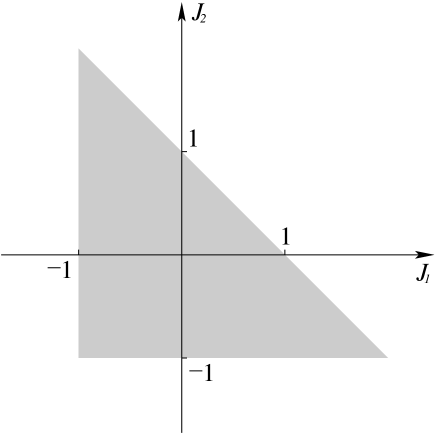
Figure 5: The allowed region of $J_{1},J_{2}$, shown by the shaded area.

One can separate the conserved total norm and write the explicit Hamiltonian for the two remaining degrees of freedom. Let us label the actions and phases of the oscillators $n,n+1,n+2$ by $i=1,2,3$, respectively. Then the corresponding canonical transformation is determined by

$$\begin{split}&I=I_{1}+I_{2}+I_{3},\quad\phi=\frac{\phi_{1}+\phi_{2}+\phi_{3}}{3},\\ &\frac{I}{3}\,{J}_{1}=\frac{2I_{1}-I_{2}-I_{3}}{3},\quad\varphi_{1}=\phi_{1}-\phi_{2},\\ &\frac{I}{3}\,{J}_{2}=\frac{I_{1}+I_{2}-2I_{3}}{3},\quad\varphi_{2}=\phi_{2}-\phi_{3}.\end{split}$$ (33)

To ensure $I_{1},I_{2},I_{3}>0$, the variables $J_{1},J_{2}$ should lie inside the triangle, shown in Fig. 5. The inverse transformation is

$$\begin{split}&\psi_{1}=\sqrt{(1+J_{1})I/3}\,e^{i(-2\varphi_{1}+\varphi_{2})/3-i\phi},\\ &\psi_{2}=\sqrt{(1-J_{1}-J_{2})I/3}\,e^{i(\varphi_{1}+\varphi_{2})/3-i\phi},\\ &\psi_{3}=\sqrt{(1+J_{2})I/3}\,e^{i(\varphi_{1}-2\varphi_{2})/3-i\phi}.\end{split}$$ (34)

The rescaled Hamiltonian for the degrees of freedom $(J_{1},\varphi_{1},J_{2},\varphi_{2})$ is given by

$$\begin{split}\frac{H-\bar{\omega}{I}}{(I/2\bar{\omega})^{2}}={}&{}(2\Omega+\Omega^{\prime}-2/3)J_{1}+(\Omega+2\Omega^{\prime}-2/3)J_{2}\\ {}&{}-\frac{2}{3}\sqrt{(1+J_{1})(1-J_{1}-J_{2})}\,(2-J_{2})\cos\varphi_{1}\\ {}&{}+\frac{1}{3}\,(1+J_{1})(1-J_{1}-J_{2})\cos{2}\varphi_{1}\\ {}&{}-\frac{2}{3}\sqrt{(1-J_{2})(1-J_{1}+J_{2})}\,(2-J_{1})\cos\varphi_{2}\\ {}&{}+\frac{1}{3}\,(1-J_{2})(1-J_{1}+J_{2})\cos{2}\varphi_{2}\\ {}&{}+\frac{7}{3}-\frac{2}{3}\,J_{1}J_{2}.\end{split}$$ (35)

Still, due to the presence of trigonometric functions, the numerical integration of the equations of motion for this Hamiltonian would be less efficient than for the polynomial Hamiltonian (7) with three degrees of freedom.

Appendix B Numerical criterion for chaos

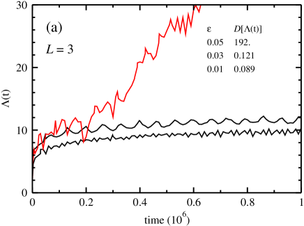
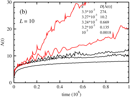
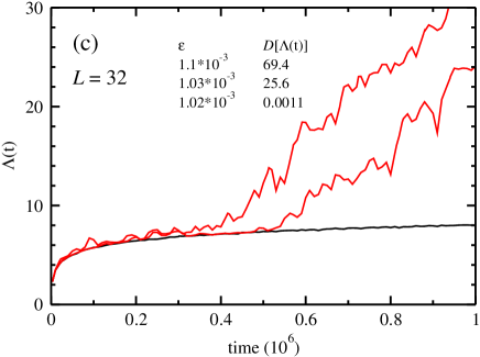
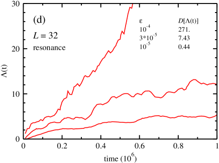
Figure 6: (color online) $\Lambda(t)$ for $0<t<10^{6}$. Panels (a), (b), (c) correspond to three chain lengths: (a) $L=3$, (b) $L=10$, (c) $L=32$. All curves on a given panel correspond to the same realization of the disorder $\{\omega_{n}^{2}\}$, phases $\{\phi_{n}\}$, and differ only by the value of $\epsilon_{n}=\epsilon$. Higher curves correspond to larger values of $\epsilon$. Panel (d) corresponds to $L=32$, but the disorder realization was artificially modified by setting $\omega_{12}=\omega_{13}=\omega_{14}$, thereby creating two neighboring resonances.

The numerical criterion for the chaotic motion used in the present work is based on the analysis of $\Lambda(t)=\ln\frac{d(t)}{d(0)}$, where $d(t)$ is the distance between points belonging to two initially close trajectories. To illustrate the idea, we plot several traces $\Lambda(t)$ in Fig. 6. Looking at them, it is quite easy to guess which curve corresponds to a regular motion, and which one to chaotic. The only exception is the lowest curve in Fig. 6(d). We know it should be chaotic, as the corresponding realization of $\{\omega_{n}^{2}\}$ contains two neighboring resonances, introduced “by hands”. However, at $\epsilon=10^{-5}$ energy exchange between the oscillators is so slow, that following their dynamics up to $T=10^{6}$ is insufficient to distinguish between regular and chaotic motion. This gives us the lower boundary on $\epsilon$. Compare also the lowest curve in Fig. 6(c) and the middle curve in Fig. 6(d). The former one is regular and the latter is chaotic, even though they have close values of $\Lambda(t=T)$. Thus, the fixed cutoff for the Lyapunov exponent (independent of $L$ and $\epsilon$), which was used in Ref. Pikovsky2011 , as the criterion for chaos, may introduce systematic errors and affect the scaling.

The main observation from Fig. 6 is that for chaotic trajectories $\Lambda(t)$ grows linearly on the average, corresponding to a finite Lyapunov exponent, while for regular trajectories

$$\Lambda(t)=\ln{t}+q_{0},$$ (36)

up to some weak noise, $q_{0}$ being some realization-dependent constant. This can be understood very simply: if two trajectories lie on neighboring invariant tori, their frequencies are only slightly different, so the phase mismatch between them is accumulated slowly and linearly in time. The distance between the trajectories is proportional to this phase mismatch, as long as the latter is small compared to unity.

To determine how well a given function $\Lambda(t)$ is approximated by the form (36) on an interval $0<t<T$, consider the time average (denoted by overline): $\overline{[\Lambda(t)-\ln{t}-q]^{2}}$. It is a quadratic function of the parameter $q$, which has a minimum at some $q$, and its value at the minimum is $D\geq{0}$. If $\Lambda(t)$ is given exactly by Eq. (36), then simply $\overline{[\Lambda(t)-\ln{t}-q]^{2}}=(q-q_{0})^{2}$, so $D=0$. Thus, the value at the minimum, given by

$$D[\Lambda(t)]=\overline{[\Lambda(t)-\ln{t}]^{2}}-\left(\overline{[\Lambda(t)-\ln{t}]}\right)^{2},$$ (37)

measures the quality of the fit of $\Lambda(t)$ by the expression (36). $D[\Lambda(t)]$ for all curves in Fig. 6 is shown on the corresponding panel. Thus, we consider the motion as regular if $D[\Lambda(t)]<1$ and chaotic otherwise.

When the Lyapunov exponent $\sigma>0$, it sets the natural upper time limit for the numerical integration of the differential equations. Indeed, when the double-precision machine zero, $2^{-52}$, multiplied by $e^{\sigma{t}}$ becomes of the order of unity, the integration inevitably deviates from the original trajectory, no matter how good the integration scheme is. This corresponds to $\Lambda=\ln{2}^{52}\approx{36}$. To check this, we have performed the time-reversal test: at time $t=t_{*}$, we invert all the momenta, and integrate up to $t=2t_{*}$. Ideally, the system should return to its initial condition. This was found to be the case if $\Lambda(t_{*})<25-30$ (for many trajectories whose Lyapunov exponents differed by one or two orders of magnitude). Thus, considering larger $\Lambda$ would produce the Lyapunov exponent not for a given trajectory, but its certain average over the phase space. As we are interested not in the trajectory itself, but only in whether it is chaotic or regular, we consider the very fact that $\Lambda(t)$ has reached 25 a sufficient evidence for chaos. If this happens within the integration time, $t<T$, we stop the integration, and simply set $D[\Lambda]=30$.

One could think that for every realization of the disorder $\{\omega_{n}^{2}\}$ and of the oscillator phases $\{\phi_{n}\}$ exists a threshold value $\epsilon_{c}$, such that for $\epsilon<\epsilon_{c}$ the motion is quasiperiodic, and for $\epsilon>\epsilon_{c}$ it is chaotic. Indeed, a natural guess is that upon increase of the integrability-breaking parameter $\epsilon$ the chaotic region of the phase space should grow. This would make the calculation for the fixed-$\epsilon$ ensemble more efficient, as one would not need to probe too small or too large values of $\epsilon$. However, this guess turns out to be wrong, as seen from Fig. 7, where we plot $\ln{D}[\Lambda]$ as a function of $\epsilon$ in the vicinity of $\epsilon=10^{-3}$ for the same realization of disorder and phases as in Fig. 6(c). The flat regions on the level of $3.4\ldots=\ln{30}$ correspond to $\Lambda(t)$ reaching $25$ for $t<T$, as discussed in the previous paragraph. One can see that the conclusion about regular/chaotic character of the dynamics is little sensitive to the chosen numerical border $D=1$: had we chosen $D=5$ or $D=1/5$, the result would not change. We also note that for the particular realization, corresponding to Fig. 7, in all intervals of $\epsilon$ where the dynamics is chaotic, the Lyapunov eigenvector is confined to sites from $n=21$ to $n=26$. This is clearly related to the fact that in this realization $|\omega_{22}-\omega_{24}|\approx{0.9}\cdot{10}^{-3}$, so the observed reentrant behavior of chaos seems to occur for the same guiding resonance.

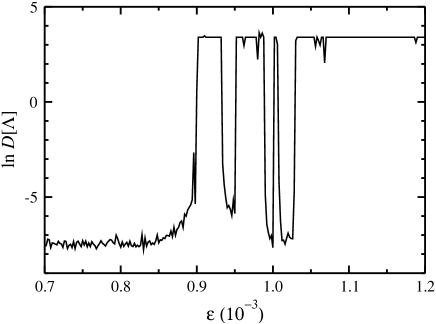
Figure 7: $\ln{D}[\Lambda]$ [with $D$ defined in Eq. (37)] as a function of $\epsilon$ for the same realization of disorder and phases as in Fig. 6(c). The upper cutoff corresponds to $\ln{30}$, as discussed in the text.

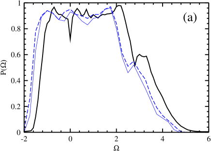
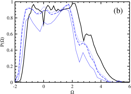
Figure 8: (color online) The phase-averaged chaotic fraction $P(\Omega)$ for a given realization of disorder on a chain with $L=32$ and frequencies $\omega_{12},\omega_{13},\omega_{14}$ chosen according to Eq. (38), for (a) $\epsilon=10^{-4}$, (b) $\epsilon=0.3\cdot{10}^{-4}$. The thick solid line on both panels corresponds to the calculation using the effective Hamiltonian from Eq. (7) and represents the section of Fig. 1 along the line $\Omega^{\prime}=0$. The thin solid, dashed and dotted lines correspond to $T=10^{6},\,3\cdot{10}^{6},\,5\cdot{10}^{6}$, respectively [the last curve is present only on panel (b)].

To check how the results are affected by the choice of the integration time $T$, we take the same realization of disorder as for the trajectories in Fig. 6 (the chain length $L=32$), and set “by hands” three nearby frequencies to be

$$\omega_{12}=\bar{\omega}+\frac{9}{4}\,\frac{\epsilon}{\bar{\omega}^{3}}\,\Omega,\quad\omega_{13}=\bar{\omega}-\frac{9}{4}\,\frac{\epsilon}{\bar{\omega}^{3}}\,\Omega,\quad\omega_{14}=\bar{\omega},$$ (38)

with a fixed $\bar{\omega}=\sqrt{0.7}$, two values of $\epsilon=10^{-4},\,0.3\cdot{10}^{-4}$, and $\Omega$ varying in the interval $-2<\Omega<6$. This chain is supposed to be well described by the effective Hamiltonian in Eq. (7) with $\Omega^{\prime}=0$. On the two panels of Fig. 8 we plot the phase-averaged chaotic fraction as a function of $\Omega$ for the two above-mentioned values of $\epsilon$, and for $T=10^{6},\,3\cdot{10}^{6},\,5\cdot{10}^{6}$, together with the result of the calculation using Eq. (7) (the section of Fig. 1 along the line $\Omega^{\prime}=0$). For both values of $\epsilon$, as $T$ is increased, the curves approach the result of Eq. (7), up to an overall horizontal shift. This horizontal shift appears because Eq. (38) neglects the nonlinear frequency shift for the oscillators with $n=12$ and 14 due to their coupling to the oscillators with $n=11$ and $15$, respectively [the difference between primed and unprimed frequencies in Eq. (LABEL:omegaprime=)]. This is also the reason why the dip at $\Omega=0$ for the result of Eq. (7) is not resolved on the curves for the long chain. What is important, is that while at $\epsilon=10^{-4}$ the integration time $T=10^{6}$ is sufficient, for $\epsilon=0.3\cdot{10}^{-4}$ integration up to $T=10^{6}$ clearly underestimates the chaotic fraction, so that $T=3\cdot{10}^{6}$ is required.

Finally, we mention that the numerical integration of the differential equations was performed using (i) the fourth-order Runge-Kutta method for the calculations reported in this section, and (ii) Bulirsch-Stoer method with polynomial extrapolation for the accumulation of statistics. The latter method turns out to require about ten times less CPU time that the former to reach the same level of accuracy. The energy conservation was satisfied extremely well in all calculated trajectories, including those with largest Lyapunov exponents, even at times when the time-reversal test had failed. Thus, it is unlikely that use of an integration scheme which automatically respects some conservation laws of the original equations (e. g., a symplectic integrator which preserves the phase space volume) would lead to more accurate results for a given trajectory: the accuracy is lost primarily in the directions, orthogonal to conservation laws.

Appendix C Single-site excitation

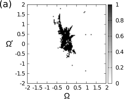
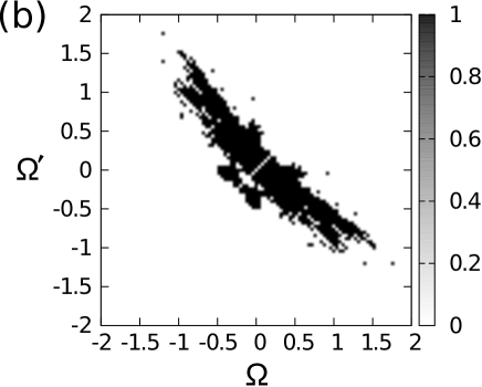
Figure 9: Values of $\Omega,\Omega^{\prime}$ for which the single-site initial conditions for the resonant triple Hamiltonian, Eq. (7), lie on a chaotic trajectory (black spots) and on a regular trajectory (white areas): (a) and (b) represent the functions $\Theta_{1}(\Omega,\Omega^{\prime})$ and $\Theta_{2}(\Omega,\Omega^{\prime})$, corresponding to the initial conditions (40a), (40b), respectively.

Let us determine the probability of chaos for an initial condition, localized on a single site,

$$p_{n}(0)=0,\quad q_{n}(0)=\delta_{n,(L+1)/2}\sqrt{2\epsilon}/\omega_{n},$$ (39)

for $L$ odd. Chaos should occur if the resonant triple contains the site $n=(L+1)/2$. Thus, the probability of chaos $P_{1}(\epsilon,L)$ should not depend on $L$ and scale as $P_{1}(\epsilon)=A_{1}\epsilon^{2}$, at large $L$ and small $\epsilon$.

To determine the coefficient $A_{1}$, we again use the effective Hamiltonian of the triple, Eq. (7), and consider two initial conditions:

$$\Psi_{1}(0)=\frac{1}{\sqrt{3}},\quad\Psi_{2}(0)=\Psi_{3}(0)=0,$$ (40a)

$$\Psi_{1}(0)=0,\quad\Psi_{2}(0)=\frac{1}{\sqrt{3}},\quad\Psi_{3}(0)=0.$$ (40b)

i. e., the excitation to be initially localized on one of the lateral sites of the triple, or on the central site. Let $\Theta_{1,2}(\Omega,\Omega^{\prime})$ equal one if the corresponding trajectory is chaotic and zero if it is regular, for each of the two initial conditions, respectively. The functions $\Theta_{1,2}(\Omega,\Omega^{\prime})$ are shown in Fig. 9. The chaotic probability is then given by

$$P_{1}(\epsilon)=81\epsilon^{2}\int\limits_{-\infty}^{\infty}d\Omega\,d\Omega^{\prime}\left[2\,\Theta_{1}(\Omega,\Omega^{\prime})+\Theta_{2}(\Omega,\Omega^{\prime})\right].$$ (41)

For the initial condition (40a), the $\Omega,\Omega^{\prime}$-integral is equal to $0.75\pm{0}.02$, while for Eq. (40b) it is equal to $1.39\pm{0.02}$, which gives $A_{1}\approx{235}$.

References

- (1) P. W. Anderson, Phys. Rev. 109, 1492 (1958).
- (2) A. Lagendijk, B. A. van Tiggelen and D. S. Wiersma, Phys. Today 62, 24 (2009).
- (3) M. B. Gertsenshtein and V. B. Vasil’ev, Theory of Probability and its Applications 4, 391 (1959).
- (4) F. Evers and A. D. Mirlin, Rev. Mod. Phys. 80, 1355 (2008).
- (5) S. Fishman, Y. Krivolapov, and A. Soffer, Nonlinearity 25, R53 (2012).
- (6) D. L. Shepelyansky, Phys. Rev. Lett. 70, 1787 (1993).
- (7) A. S. Pikovsky and D. L. Shepelyansky, Phys. Rev. Lett. 100, 094101 (2008).
- (8) S. Flach, D. O. Krimer, and Ch. Skokos, Phys. Rev. Lett. 102, 024101 (2009).
- (9) J. D. Bodyfelt, T. V. Laptyeva, Ch. Skokos, D. O. Krimer, and S. Flach, Phys. Rev. E 84, 016205 (2011).
- (10) W.-M. Wang and Z. Zhang, J. Stat. Phys. 134, 953 (2009).
- (11) S. Fishman, Y. Krivolapov, and A. Soffer, Nonlinearity 22, 2861 (2009).
- (12) M. Mulansky, K. Ahnert, and A. Pikovsky, Phys. Rev. E 83, 026205 (2011).
- (13) E. Michaely and S. Fishman, Phys. Rev. E 85, 046218 (2012).
- (14) B. V. Chirikov, Phys. Rep. 52, 263 (1979).
- (15) G. M. Zaslavsky, Chaos in Dynamic Systems, (Harwood Academic Publishers, Newark, 1985).
- (16) A. J. Lichtenberg and M. A. Lieberman, Regular and Chaotic Dynamics (Springer-Verlag, New York, 1992), 2nd ed.
- (17) J. Fröhlich, T. Spencer, and C. E. Wayne, J. Stat. Phys. 42, 247 (1986).
- (18) M. Johansson, G. Kopidakis, and S. Aubry, Europhys. Lett. 91, 50001 (2010).
- (19) D. M. Basko, Ann. Phys. 326, 1577 (2011).
- (20) A. Pikovsky and S. Fishman, Phys. Rev. E 83, 025201(R) (2011).
- (21) V. Oganesyan, A. Pal, and D. A. Huse, Phys. Rev. B 80, 115104 (2009).
- (22) M. V. Ivanchenko, T. V. Laptyeva, and S. Flach, Phys. Rev. Lett. 107, 240602 (2011).
- (23) Strictly speaking, does not correspond to the total energy per oscillator, as it does not include , the second term of Eq. (LABEL:HFSW=). In particular, this means that (i) the sum of all , corresponding to is not conserved during the evolution, and (ii) Eq. (4) with the -function replaced by the exponential is not exactly the thermal distribution. However, and , so represents a small correction at , and indeed has the meaning of temperature in the thermal ensemble.
- (24) This is because the system (LABEL:HFSW=) has only one integral of motion (energy), which should be contrasted with DNLS which has two integrals of motion (energy and norm), so the minimal number of oscillators needed to produce chaos in DNLS is three.
- (25) M. Mulansky, K. Ahnert, A. Pikovsky and D. L. Shepelyansky, J. Stat. Phys. 145, 1256 (2011).