Effective Models for Statistical Studies of Galaxy-Scale Gravitational Lensing

Abstract

We have worked out simple analytical formulae that accurately approximate the relationship between the position of the source with respect to the lens center and the amplification of the images, hence the lens cross section, for realistic lens profiles. We find that, for essentially the full range of parameters either observationally determined or yielded by numerical simulations, the combination of dark matter and star distribution can be very well described, for lens radii relevant to strong lensing, by a simple power-law whose slope is very weakly dependent on the parameters characterizing the global matter surface density profile and close to isothermal in agreement with direct estimates for individual lens galaxies. Our simple treatment allows an easy insight into the role of the different ingredients that determine the lens cross section and the distribution of gravitational amplifications. They also ease the reconstruction of the lens mass distribution from the observed images and, vice-versa, allow a fast application of ray-tracing techniques to model the effect of lensing on a variety of source structures. The maximum amplification depends primarily on the source size. Amplifications larger than $\approx 20$ are indicative of compact source sizes at high-$z$, in agreement with expectations if galaxies formed most of their stars during the dissipative collapse of cold gas. Our formalism has allowed us to reproduce the counts of strongly lensed galaxies found in the H-ATLAS SDP field. While our analysis is focussed on spherical lenses, we also discuss the effect of ellipticity and the case of late-type lenses (showing why they are much less common, even though late-type galaxies are more numerous). Furthermore we discuss the effect of a cluster halo surrounding the early-type lens and of a supermassive black hole at its center.

1. Introduction

The discovery rate of strong galaxy-scale lens systems has increased dramatically in recent years mostly thanks to spectroscopic lens searches and, most recently, to surveys of sub-millimeter galaxies. Spectroscopic searches, such as the Sloan Lens Advanced Camera for Surveys (SLACS) survey (Bolton et al. 2006, 2008; Auger et al. 2009) or the BOSS (Baryon Oscillation Spectroscopic Survey) Emission-Line Lens Survey (BELLS; Brownstein et al. 2012) or the optimal line-of-sight (OLS) lens survey (Willis et al. 2006) or the Sloan WFC (Wide Field Camera) Edge-on Late-type Lens Survey (SWELLS; Treu et al. 2011), rely on the detection of multiple background emission lines in the residual spectra found after subtracting best-fit galaxy templates to the foreground-galaxy spectrum.

Sub-millimeter surveys were predicted (Blain 1996; Perrotta et al. 2002, 2003; Negrello et al. 2007), and demonstrated (Negrello et al. 2010), to be an especially effective route to efficiently detect strongly lensed galaxies at high redshift because the extreme steepness of number counts of unlensed high-$z$ galaxies implies a strong magnification bias so that they are easily exceeded by those of strongly lensed galaxies at the bright end. Also, gravitational lensing effects are more pronounced for more distant sources. But high-$z$ galaxies are frequently in a dust-enshrouded active star formation phase and therefore are more easily detected at far-IR/sub-mm wavelengths, while they are very optically faint. Negrello et al. (2007) predicted that about 50% of galaxies with $500\,\mu$m flux densities above $\approx 100\,$mJy would be strongly lensed, with the remainder easily identifiable as local galaxies or as radio-loud Active Galactic Nuclei (AGNs). This prediction was supported by the mm-wave South Pole Telescope (SPT) counts (Vieira et al. 2010). But a spectacular confirmation came with the results of the Herschel Astrophysical Terahertz Large Area Survey (H-ATLAS; Eales et al. 2010) for the Science Demonstration Phase (SDP) field covering about $14.4$ deg². Five out of the 10 extragalactic sources with $S_{500\,\mu\rm m}\gtrsim 100\,$mJy were found to be strongly lensed high-$z$ galaxies, four are $z<0.1$ spiral galaxies and one is a flat-spectrum radio quasar (Negrello et al. 2010). Gonzalez-Nuevo et al. (2012) presented a simple method, the Herschel-ATLAS Lensed Objects Selection (HALOS), aimed at identifying fainter strongly lensed galaxies. This method gives the prospect of reaching a surface density of $\sim 2$ deg^-2 for strongly lensed candidates, i.e., the detection of $\sim 1000$ high-$z$ strongly lensed galaxies over the full H-ATLAS survey area ($\approx 550$ deg²; Eales et al. 2010).

It should be noted that the (sub-)mm selected lensed galaxies are very faint in the optical, while most foreground lenses are passive ellipticals (Auger et al. 2009; Negrello et al. 2010), essentially invisible at sub-mm wavelengths. This means that the foreground lens is ‘transparent’ at (sub-)mm wavelengths, i.e. does not confuse the images of the background source. Therefore, the (sub-)mm selection shares with spectroscopic searches the capability of detecting lensing events with small impact parameters and has the advantage that, in most cases, there is no need to subtract the lens contribution to recover the source images within the effective radii of the lenses. Also, compared to the optical selection, the (sub-)mm selection allows us to probe earlier phases of galaxy evolution which have typically higher lensing optical depths. This makes this technique ideal for tracing the mass density profiles of elliptical galaxies over a broad redshift range and for probing their evolution with cosmic time.

Samples of strongly lensed galaxies are further enriched by the, to some extent complementary, imaging surveys (Cabanac et al. 2007; Faure et al. 2008; Kubo & Dell’ Antonio 2008; Ruff et al. 2011) which look for arc-like features, and by radio surveys (Browne et al. 2003). All that holds the promise of a fast increase of the number of known strongly lensed sources, fostered by the forthcoming large area optical (e.g., Oguri & Marshall 2010) and radio (SKA, Square Kilometer Array) surveys (e.g., Koopmans, Browne, & Jackson 2004). A simple, efficient, analytical tool applicable to the analysis of large samples of galaxy-scale lenses is therefore warranted.

In this paper we work out exact and approximate solutions of the lens equation based on a realistic model for the mass density profile of the lens (§ 2) and exploit them to reckon the lensing probability as a function of the source redshift (§ 3). As an application of these results, following on the study of the high-$z$ luminosity function of galaxies measured by the H-ATLAS survey (Lapi et al. 2011), we compute, in § 4, the number counts of strongly lensed sub-mm galaxies implied by the physical model of galaxy formation and evolution formulated by Granato et al. (2004) and further developed by Lapi et al. (2006) and Mao et al. (2007). The model counts are compared with the observational estimates by Negrello et al. (2010) and by Gonzalez-Nuevo et al. (2012). While our study is focussed on early-type lenses, assumed to be circularly symmetric, the cases of late-type lenses, of ellipticity, of the presence of a super-massive black hole in the galactic nucleus, and of super-galactic structures are discussed in § 5. Finally, our main results are summarized in § 6.

Throughout the paper we adopt the standard flat $\Lambda$CDM cosmology (see Komatsu et al. 2011) with current matter density parameter $\Omega_{\rm M}=0.27$ and Hubble constant $H_{0}=72$ km s^-1 Mpc^-1.

2. Lensing cross section

2.1. Lens mass models

We focus here on galaxy-scale lensing, i.e., on those lensing events where the deflector is a single/isolated early-type galaxy. The discussion of the effect of the more extended dark matter (DM) halo of a group or cluster in which the lens galaxy may reside, or of the disk of later type galaxies is deferred to § 5.

More specifically, we assume that the lens galaxy is associated to a DM halo of mass $M_{\rm H}$ in the range $10^{11.4}-10^{13.5}\,M_{\odot}$ virialized at redshift $z_{\ell,v}\gtrsim 1.5$. The redshift and the lower mass limit are crudely meant to single out galactic halos associated with individual spheroidal galaxies. Disk-dominated (and irregular) galaxies are primarily associated with halos virializing at $z_{\ell,v}\lesssim 1.5$, which may have incorporated halos less massive than $10^{11.4}\,M_{\odot}$ virialized at earlier times, that form their bulges. The upper mass limit to individual galaxy halos comes from weak-lensing observations (e.g., Kochanek & White 2001; Kleinheinrich et al. 2005), kinematic measurements (e.g., Kronawitter et al. 2000; Gerhard et al. 2001), and from a theoretical analysis on the velocity dispersion function of spheroidal galaxies (Cirasuolo et al. 2005). The same limit is also suggested by modeling of the spheroids mass function (Granato et al. 2004), of the quasar luminosity functions (Lapi et al. 2006), and of the sub-mm galaxy number counts (Lapi et al. 2011).

For the DM we adopt a standard NFW (Navarro, Frenk, & White 1996) profile (e.g., Lokas & Mamon 2001)

$$\rho_{\rm H}(r)={M_{\rm H}\over 4\pi R_{\rm H}^{3}}\,{f_{c}\,c^{2}\over(r/R_{\rm H})\,(1+c\,r/R_{\rm H})^{2}},$$ (1)

where $c$ is the concentration parameter and $f_{c}\equiv[\log(1+c)-c/(1+c)]^{-1}$. The halo virial radius $R_{\rm H}$ is given by (e.g., Bryan & Norman 1998; Barkana & Loeb 2001)

$$R_{\rm H}=62\,\left({M_{\rm H}\over 10^{12}\,M_{\odot}}\right)^{1/3}\,\left[{\Omega_{\rm M}\over\Omega_{\rm M}(z_{\ell,v})}\,{\Delta_{v}(z_{\ell,v})\over 18\pi^{2}}\right]^{-1/3}\,\left({1+z_{\ell,v}\over 3.5}\right)^{-1}~{}\mathrm{kpc},$$ (2)

in terms of the virialization redshift of the lens $z_{\ell,v}$, of the evolved density parameter $\Omega_{\rm M}(z)=\Omega_{\rm M}\,(1+z)^{3}/[\Omega_{\rm M}\,(1+z)^{3}+1-\Omega_{\rm M}]$, and of the overdensity threshold for virialization $\Delta_{v}(z)=18\,\pi^{2}+82\,[\Omega_{\rm M}(z)-1]-39\,[\Omega_{\rm M}(z)-1]^{2}$. For example, $z_{\ell,v}=2.5$ and $M_{\rm H}=10^{13}\,M_{\odot}$ correspond to a virial size $R_{\rm H}\approx 200\,$kpc. Since the NFW profile yields a logarithmically diverging mass, we set the edge of the halo at $R_{\rm H}$.

Hereafter we adopt $z_{\ell,v}=2.5$ as our fiducial value. This choice is motivated on considering that massive early-type galaxies at $z_{\ell}\sim 0.7$ feature relatively old ages $\sim 3-5$ Gyr of their stellar populations, and formed the bulk of their stars over a timescale of order $1$ Gyr (for a review, see Renzini 2006; also Lapi et al. 2011). These evidences point toward a virialization redshift of the host halo in the range $z_{\ell,v}\sim 1.5-3.5$, consistent with the distribution of creation redshifts found in numerical simulations for the massive halos considered here (e.g., Moreno et al. 2009). Note that for an early-type lens the observation redshift ($z_{\ell}\sim 0.7$; González-Nuevo et al. 2012) is, generally, substantially lower than the virialization one ($z_{\ell,v}\sim 2.5$). Therefore the frequently made approximation $z_{\ell}\approx z_{\ell,v}$ leads to a large overestimate of the halo size and, indirectly, to an underestimate of the lensing probability.

Numerical simulations indicate that the concentration $c$ depends on halo mass and redshift as (Prada et al. 2011)

$$c\approx 5\,\left({M_{\rm H}\over 10^{13}\,M_{\odot}}\right)^{-0.074}\,\left({1+z_{\ell}\over 1.7}\right)^{-1},$$ (3)

with a scatter of about $20\%$. For a lens with $M_{\rm H}=10^{13}\,M_{\odot}$ at redshift $z_{\ell}=0.7$ we have $c\approx 5$, that we adopt as our fiducial value.

The DM to baryon ratio $M_{\rm H}/M_{\star}$ in early-type galaxies is generally in the range $10-70$. In fact, this quantity can be roughly bounded from below by the cosmological DM to baryon mass ratio (see Komatsu et al. 2011) that takes on values around $6$, and from above by the DM to stellar mass ratio that statistical arguments (see Shankar et al. 2006; Lagattuta et al. 2010; Moster et al. 2010) estimate to be around $70$. We take $M_{\rm H}/M_{\star}=30$ as our fiducial value.

The impact on the lensing probability of different choices for $z_{\ell,v}$, for $c$ [including the use of the halo-mass dependent expression of Eq. (3)], and for $M_{\rm H}/M_{\star}$ is discussed in § 3.

For the stellar component we adopt the 3-D Sérsic profile (Prugniel & Simien 1997)

$$\rho_{\star}(r)={M_{\star}\over 4\pi R_{e}^{3}}\,{b_{n}^{2n}\over n\Gamma(2n)}\,\left({r\over R_{e}}\right)^{-\alpha_{n}}\,e^{-b_{n}\,(r/R_{e})^{1/n}},$$ (4)

where $R_{e}$ is the effective radius, $n$ is the Sérsic index, $b_{n}\equiv 2\,n-1/3+0.009876/n$, and $\alpha_{n}\equiv 1-1.188/2\,n+0.22/4\,n^{2}$.

The effective radius $R_{e}$ is related to the stellar mass by (Shen et al. 2003; Hyde & Bernardi 2009)

$$R_{e}\approx 1.28\,\left({M_{\star}\over 10^{10}\,M_{\odot}}\right)^{0.55}~{}\mathrm{kpc},$$ (5)

found to hold (with a $\approx 30\%$ scatter) for $z_{\ell}\lesssim 1$. Several recent observational studies have found that massive, passively evolving galaxies at $z\gtrsim 1$ are much more compact than local galaxies of similar stellar mass (Fan et al. 2010 and references therein). The study by Maier et al. (2009), with high spectroscopic completeness, finds however that the size evolution at fixed mass is modest ($\sim 25\%$) from $z\sim 0.7$ to $z=0$, i.e. up to our reference value of the lens redshift. We have checked that decreasing $R_{e}$ at fixed $M_{\star}$ by a factor $f_{e}>1$ increases somewhat the probability of amplifications only in the range $3\lesssim\mu\lesssim 5$; the effect becomes essentially independent of the decrease factor for $f_{e}\gtrsim 1.5$.

Values of the Sérsic index for massive early-type galaxies are in the range $n\approx 3-10$, with a tendency for more massive systems to feature higher values (e.g., Kormendy et al. 2009). Early-type galaxies with $n=2$ generally are either dwarf spheroidals or contain a substantial disk component and do not obey Eq. (5). We will consider a fiducial value $n=4$, corresponding to the classical de Vaucouleurs (1948) profile. Again, the effect on the lensing probability of different values is investigated in § 3.

To sum up, we adopt a two-component model, made of a stellar component with a Sérsic profile plus a DM halo with a NFW profile. Given the halo mass $M_{\rm H}$ and the virialization redshift, $z_{\ell,v}$, the total mass distribution of the lens galaxy is specified by the parameters $z_{\ell}$, $M_{\rm H}/M_{\star}$, and $n$ [after Eq. (3) $c$ is determined by $M_{\rm H}$ and $z_{\ell}$]. Hereafter this two-component model will be referred to as the ‘SISSA model’. The lensing probability distribution yielded by this model will be compared with those yielded by two other commonly used models. The first (hereafter referred to as ‘NFW model’) just consists in adopting a pure NFW profile, hence neglecting the effect of the baryons. The second (hereafter referred to as the ‘SIS model’) adopts the classic singular isothermal sphere density profile

$$\rho_{\rm SIS}(r)={\sigma_{\rm SIS}^{2}\over 2\pi\,G}\,{1\over r^{2}}={M_{\rm H}\over 4\pi R_{\rm H}^{3}}\,\left({r\over R_{\rm H}}\right)^{-2},$$ (6)

where $\sigma_{\rm SIS}$ is the 1-D velocity dispersion of the overall mass. The second equality follows from the commonly used assumption $\sigma_{\rm SIS}\approx V_{\rm H}/\sqrt{2}$, in terms of the halo circular velocity $V_{\rm H}^{2}=G\,M_{\rm H}/R_{\rm H}$.

2.2. Surface density profile

The surface density writes

$$\Sigma(s)=\int{\mathrm{d}}r~{}{r\over\sqrt{r^{2}-s^{2}}}\,\rho(r),$$ (7)

$s$ being the radial coordinate projected on the plane of the sky. It is important to remember that the surface density becomes effective for strong lensing when it exceeds the critical threshold

$$\Sigma_{c}={c^{2}\over 4\pi\,G}\,{(1+z_{\ell})\,D_{s}\over D_{\ell}\,D_{\ell s}}$$ (8)

corresponding to a convergence $\kappa=1$ for a thin lens. Here $D_{s}$, $D_{\ell}$, and $D_{\ell s}=D_{s}-D_{\ell}$ are the comoving angular distances (also called proper motion distances; see Kochanek 2006) from the source at $z_{s}$ to the observer at $z=0$, from the lens at $z_{\ell}$ to the observer at $z=0$, and from the source at $z_{s}$ to the lens at $z_{\ell}$, respectively. In a flat Universe the comoving angular distances are defined as $D_{ij}\equiv(c/H_{0})\,\int_{z_{i}}^{z_{j}}{\rm d}z\,[\Omega_{M}\,(1+z)^{3}+1-\Omega_{M}]^{-1/2}$. The angular diameter distance is $D_{ij}/(1+z_{j})$ and the luminosity distance is $D_{ij}\,(1+z_{j})$.

In Fig. 1 the surface mass density yielded by the SISSA model for a lens at $z_{\ell}=0.7$ with $M_{\rm H}=10^{13}\,M_{\odot}$, $z_{\ell,v}=2.5$, $c=5$, $n=4$, and $M_{\rm H}/M_{\star}=30$, is compared with those yielded by the Sérsic, NFW and SIS laws. The horizontal grey line represents the critical surface density when the source is at $z_{s}=2.5$ and the lens at $z_{\ell}=0.7$. It shows that, in this case, only the matter located at $s\lesssim 10^{-1.5}\,R_{\rm H}$ is effective for strong lensing. The stellar contribution to the surface density dominates for $s\lesssim 10^{-2}\,R_{\rm H}$, while the DM contribution takes over at larger radii.

As illustrated by Fig. 1 in the radial range $-2.5\lesssim\log(s/R_{\rm H})\lesssim-1$, which generally contributes most to the gravitational deflection, the combination of the stellar and DM components to the total surface density closely mimics a power law

$$\Sigma(s)=\Sigma_{0}\,\left({s\over s_{0}}\right)^{-\eta}.$$ (9)

In Table 1 we show that, at fixed halo mass, $M_{\rm H}$, both the normalization $\Sigma_{0}$ at the reference radius $s_{0}\approx 10^{-2}\,R_{\rm H}$, and the power-law index $\eta\approx 0.8-0.9$ are only weakly dependent on the parameters of the mass distribution. Specifically, $\eta$ and $\Sigma_{0}$ slightly increase with decreasing $M_{\rm H}/M_{\star}$ (i.e. for higher stellar contributions in the inner region), with increasing halo concentration (i.e. for a higher DM contribution in the inner region), and with decreasing Sérsic index (i.e. for a stellar distribution more concentrated at the center). At fixed parameters of the lens mass distribution, $\Sigma_{0}$ (obviously) decreases while $\eta$ increases with decreasing halo mass.

The slopes of the power-law approximation are in good agreement with those determined from the stellar dynamics (e.g., Thomas et al. 2011), from the globular cluster/planetary nebulae kinematics (e.g., Rodionov & Athanassoula 2011), from the HI gas disk/ring (e.g., Weijmans et al. 2008), from the profile of the X-ray emission (e.g., Churazov et al. 2010; Humphrey & Buote 2010), and from gravitational lensing in individual galaxies (e.g., Koopmans et al. 2009; Spiniello et al. 2011; Barnabé et al. 2011). All these observational determinations concur in indicating that the overall density profile is roughly isothermal (at least in the inner region), with surface density slopes around $\eta\approx 1$.

In comparing the observational determinations of the slopes of the density profiles it must be kept in mind that the profiles are not real power laws. This implies that the slope of the volume density, $\eta_{V}$, is not simply related to the slope of the surface density, $\eta$, by $\eta_{V}=\eta+1$, as in the power-law case. For the combination of Sérsic and NFW profiles considered here we find that the best fit slopes over the radial range relevant for strong lensing are related by $\eta_{V}\approx\eta+1.2$, due to projection effects. Thus, the slightly under-isothermal values of $\eta$ yielded by the SISSA model (see Table 1) are fully consistent with the slightly over-isothermal values of $\eta_{V}$ (in the range $1.9-2.3$) found by Koopmans et al. (2009) and Barnabé et al. (2011). The latter authors also find hints of a steeper slope $\eta$ for the least massive systems, consistent with the trend coming out of Table 1. Finally, note that during the galaxy lifetime the mass density profile may evolve under the influence of various physical processes; we address the issue in § 5.3.

2.3. Lens equation: exact and approximated solutions

In the following we consider circular lenses, deferring to § 5 the discussion on the effect of ellipticity. In such a case, the light rays coming from a distant, point-like source are deflected by an angle

$$\alpha(\theta|z_{\ell},z_{s})={2\over\theta}\,\int_{0}^{\theta}{\rm d}\vartheta\,\vartheta\,{\Sigma(s)\over\Sigma_{c}}={4G\,M(<\xi)\over c^{2}\,\xi}\,{D_{\ell s}\over D_{s}},$$ (10)

where $\theta$ is the angular distance of the image from the lens center, $\vartheta\equiv s\,(1+z_{\ell})/D_{\ell}$, and $M(<\xi)\equiv 2\pi\int_{0}^{\xi}{\rm d}s\,s\,\Sigma(s)$ is the mass within the projected radius $\xi=\theta D_{\ell}/(1+z_{\ell})$.

The relation between the position of the source and of its (possibly multiple) lensed image(s) relative to the observer is described by the lens equation

$$\beta=\theta-{\theta\over|\theta|}\,\alpha(|\theta|).$$ (11)

Here $\beta$ and $\theta$ are the angles formed by the source and by its images with the optical axis, i.e. with the imaginary line connecting the observer and the center of the lens mass distribution. Solving the lens equation means finding all the positions $\theta$ of the images for a given source position $\beta$.

The amplification of the images can be computed as:

$$\mu={1\over\lambda_{+}\,\lambda_{-}}~{}~{}~{}~{}\mathrm{with}~{}~{}\lambda_{+}\equiv 1-{{\rm d}\alpha\over{\rm d}\theta}~{}~{}\mathrm{and}~{}~{}\lambda_{-}\equiv 1-{\alpha\over\theta}.$$ (12)

If either of the two quantities $\lambda_{\pm}$ vanishes, the magnification formally diverges. Thus the condition $\lambda_{\pm}=0$ defines critical curves in the lens plane and corresponding caustics in the source plane. The magnification can be positive or negative, implying that the image has positive or negative parity or, equivalently, is direct or reversed. The total magnification $\mu_{\rm tot}$ is the sum of the absolute values of the magnifications for all the images, i.e., ignoring parity.

A point-like source perfectly aligned with the observer and the center of the foreground mass distribution is lensed into a ring of radius $\theta_{E}$, called Einstein ring. For a circular lens it coincides with the critical curve defined by $\lambda_{-}=0$. The other critical curve defined by $\lambda_{+}=0$, if present, approximately coincides with an inner ring of radius $\theta_{I}<\theta_{E}$. In Fig. 2 we show an example of the numerical solutions of the lens equation for the SISSA model. The source is located at redshift $z_{s}=2.5$ and the lens at redshift $z_{\ell}=0.7$. The parameters of the lens mass distribution are as in Fig. 1. The Einstein ring is located at $\theta_{E}\approx 1.82^{\prime\prime}$. In addition, the SISSA model (and also the NFW model, but not the SIS model) features another, inner critical curve at $\theta_{I}\approx 0.32^{\prime\prime}$. In the top panel we illustrate the relation between the angular positions of the source $\beta$ and of the images $\theta$, normalized to the position $\theta_{E}$ of the Einstein ring. In the bottom panel, we illustrate the relation between the angular position of the source $\beta$ and the amplification of the different images, including the total magnification summed over them.

As it can be seen from the bottom panel of Fig. 2, the SISSA model features one image for $\beta\gtrsim\beta_{I}$ and three images for $\beta\lesssim\beta_{I}$, where $\beta_{I}\approx 0.5\,\theta_{E}$ is the location of the outer caustic corresponding to the inner critical curve at $\theta_{I}$. Of the three images, however, the one closest to the optical axis (dot-dashed line) is strongly demagnified, while the other two (solid and dashed lines) are amplified by different amounts and feature opposite parity. At the location of the outer caustic $\beta=\beta_{I}$, the second and third images are degenerate with infinite magnification (in the plot the red solid curve referring to the total magnification should go to $\mu\rightarrow\infty$ at $\beta=\beta_{I}$, but the divergence has been smoothed out for clarity).

In Fig. 3 we illustrate how the angular positions of the Einstein ring $\theta_{E}$ and of the inner critical curve $\theta_{I}$ depend on the lens mass and redshift. In the top panel we focus on the SISSA model, and show how the position of the Einstein ring and of the inner critical curve vary as a function of the lens redshift $z_{\ell}$, for different source redshifts $z_{s}$. The bottom panel elucidates the dependence of $\theta_{E}$ and $\theta_{I}$ on the lens mass for different lens models, at fixed $z_{s}=2.5$ and $z_{\ell}=0.7$. Plainly, $\theta_{E}$ and $\theta_{I}$ increase with the halo mass since, after Eq. (10), more mass implies wider bend angles. The SISSA model yields larger values of $\theta_{E}$ than the NFW and SIS models but smaller values of $\theta_{I}$ than the NFW model (the SIS model has no inner critical curve).

These behaviors, and the comparisons among different mass models, may be better understood looking at approximate solutions of the lens equations obtained using the power-law description of the projected mass density [Eq. (9)] that, as shown by Fig. 1, approximates quite well a realistic density profile in the radial range most relevant for strong lensing. For the SISSA model, $\eta\approx 0.8-0.9$ is weakly dependent on the parameters of the mass distribution (see Table 1). The SIS model has a slightly steeper slope ($\eta_{\rm SIS}=1$), while, in the range most relevant for strong lensing, the NFW can be approximated with a flatter slope $\eta_{\rm NFW}\approx 0.3-0.4$.

Under the power law approximation the deflection angle due to the lens potential within a circle of angular radius $\theta$ is

$$\bar{\alpha}(\theta)=|\bar{\theta}|^{1-\eta}.$$ (13)

Here and in the following the over-bar (e.g., $\bar{\theta}\equiv\theta/\theta_{E}$) denotes normalization to the Einstein radius, that for power-law lens models can be simply written as

$$\theta_{E}=\theta_{0}\,\left({2\over 2-\eta}\,{\Sigma_{0}\over\Sigma_{c}}\right)^{1/\eta},$$ (14)

with $\theta_{0}\equiv s_{0}\,(1+z_{\ell})/D_{\ell}$ [cf. Eq. (9)]. Table 1 shows that, at fixed lens and source redshift, the factor $[2\,\Sigma_{0}/(2-\eta)\,\Sigma_{c}]^{1/\eta}$ scales approximately as $M_{\rm H}^{1/3}$, implying $\theta_{E}\propto M_{\rm H}^{2/3}$ since trivially $\theta_{0}\propto R_{\rm H}\propto M_{\rm H}^{1/3}$. This illustrates the power of lensing for weighing the halos. Since

$$\lambda_{-}=1-|\bar{\theta}|^{-\eta}~{}~{}~{}~{}~{}~{}~{}~{}\lambda_{+}=1-(1-\eta)\,|\bar{\theta}|^{-\eta}$$ (15)

the magnification of an image is

$$\mu\equiv{1\over\lambda_{+}\,\lambda_{-}}={1\over[1-|\bar{\theta}|^{-\eta}]\,[1-(1-\eta)\,|\bar{\theta}|^{-\eta}]}.$$ (16)

This equation highlights that, in addition to the critical curve corresponding to the Einstein ring ($\theta=\theta_{E}$), for $\eta<1$ there is also an inner ring at

$$\theta_{I}=\theta_{E}\,(1-\eta)^{1/\eta}.$$ (17)

To get the magnification from Eq. (16) we need to compute the positions, $\bar{\theta}$, of the images as a function of the angular distance $\bar{\beta}$ (in units of $\theta_{E}$) of the source from the optical axis by solving the lens equation

$$\bar{\beta}=\bar{\theta}\,-{\bar{\theta}\over|\bar{\theta}|}\,|\bar{\theta}|^{1-\eta}.$$ (18)

Summing up over all the images yields the global magnification of the lens model as a function of $\beta$.

For the SIS model ($\eta=1$) this gives a constant deflection $\alpha=\theta_{E}$, and no radial critical curve. For $\bar{\beta}>1$, i.e., outside $\theta_{E}$, the lens equation yields only one image at $\bar{\theta}=1+\bar{\beta}$ with magnification $\mu=1+1/\bar{\beta}$. On the other hand, for $\bar{\beta}\lesssim 1$, i.e., inside $\theta_{E}$, it gives the two images $\bar{\theta}_{\pm}=\bar{\beta}\pm 1$, and related magnifications $\mu_{\pm}=1\pm 1/\bar{\beta}$; thus the total magnification amounts to $\mu=|\mu_{+}|+|\mu_{-}|=\mu_{+}-\mu_{-}=2/\bar{\beta}$.

For a generic $\eta<1$ it is not possible to solve the lens equation analytically but we find that the numerical solutions can be well approximated, over the amplification range $1\lesssim\mu\lesssim 30$ and over the range of parameters explored in Table 1, by the expressions $\displaystyle\bar{\beta}=$ $\displaystyle 1/(\mu-1)^{\eta}~{}~{}~{}~{}~{}~{}$ $\displaystyle\mathrm{for}~{}~{}~{}\bar{\beta}\geq\bar{\beta}_{I}$ $\displaystyle\bar{\beta}=$ $\displaystyle(2/\mu)^{\eta}~{}~{}~{}~{}~{}~{}$ $\displaystyle\mathrm{for}~{}~{}~{}\bar{\beta}\leq\bar{\beta}_{I},$

that recover the SIS solutions for $\eta=1$. The value $\bar{\beta}_{I}\equiv\eta\,(1-\eta)^{-1+1/\eta}$ corresponds to the location of the inner critical curve $\theta_{I}$.

The goodness of these approximations may be appreciated by eye on looking at the dotted lines in Fig. 2 (both panels). They can be useful not only for fast computations of the lensing cross section, but also for constructing simulated lensed images of extended sources via the ray-tracing technique or, inversely, for reconstructing the lens mass profile from images of lensed sources.

2.4. Cross sections

Given the relation between the source position $\beta$ and the total magnification of the images $\mu$, the cumulative cross section for lensing magnification, as a function of the lens halo mass $M_{\rm H}$ and of the lens and source redshifts $z_{\ell}$ and $z_{s}$, simply writes:

$$\sigma(>\mu,M_{\rm H},z_{s},z_{\ell})=\pi\,\beta^{2}(\mu).$$ (20)

In Fig. 4 we illustrate the cumulative lens cross section for the SISSA, NFW and SIS models as a function of $M_{\rm H}$, for $z_{s}=2.5$, $z_{\ell}=0.7$ and two values of $\mu$. For massive halos moderate amplifications ($\mu\lesssim 5$) are mainly contributed by the outer regions of the mass distribution where the DM dominates. Thus the SISSA and the NFW models yield very similar values of the cumulative cross section for $2<\mu<5$. On the other hand, strong amplifications ($\mu>10$) are mainly contributed by inner regions where the stellar component becomes important or even dominant. Correspondingly, the SISSA cross section is considerably higher than the NFW and close to the SIS one. The different shapes of the cross sections as a function of halo mass mainly reflect the different dependencies of $\theta_{E}$ on $M_{\rm H}$ for the three models. The value of the projected radius $s_{c}$ at which the surface density equals the critical threshold for lensing, $\Sigma_{c}$ [Eq. (8)], decreases with decreasing $M_{\rm H}$, causing a decrease of the lensing cross section. In the case of the NFW model, below $\log(M_{\rm H}/M_{\odot})=12$ the radius $s_{c}$ lies in the region where the profile is much flatter than that of the SIS and SISSA models. As a consequence, it decreases faster with decreasing $M_{\rm H}$ and, correspondingly, the lens cross section drops.

2.5. Lensing by extended sources

The above results apply to the idealized case of a point-like source. What about extended sources? The problem can be solved via the ray-tracing technique (e.g., Schneider, Ehlers & Falco 1992, p. 304), i.e. by applying the $\beta-\theta$ and $\beta-\mu$ relations to every point of the unlensed light distribution of the source. Some examples are shown in Figs. 5 to 7 where $z_{s}=2.5$ and $z_{\ell}=0.7$. In the cases of Figs. 5 and 6 the light distribution of the source is modeled as a standard Sérsic profile with $n=4$, while Fig. 7 pertains to a galaxy comprising multiple (4 in this example) luminous, giant clumps that appear to be a ubiquitous feature of high-redshift star-forming galaxies (e.g., Förster Schreiber et al. 2011). The results are shown for different mass models.

Figure 5 refers to a zero impact parameter, i.e. the center of the source is aligned with the optical axis. The central regions of the source are strongly amplified and deformed into the Einstein ring. The NFW and SISSA models (but not the SIS model) yield also an inner critical curve, difficult to see because of the limited resolution of the figure. In Fig. 6 the impact parameter is small but non-null. The Einstein ring and the inner critical curve are still present since there are regions of the unlensed extended source that are crossed by the optical axis. But the central, brightest region is lensed into two deformed and amplified images, one inside and the other outside the Einstein ring. In Fig. 7 the 4 clumps have small impact parameters (specified in the caption). The lensed image looks like an Einstein ring with a knotty structure. High resolution imaging would be necessary to distinguish this configuration from that produced by a smooth source profile with an impact parameter close to zero.

This analysis also provides an useful way to estimate the maximum amplification $\mu_{\rm max}$ to be expected from extended sources, when their multiple images in the lens plane are not resolved (e.g., Peacock 1982). We compute the quantity $\mu_{\rm max}$ as the ratio between the total flux of the lensed images to that of the unlensed source over the image plane (see Perrotta et al. 2002 for details). In Fig. 8 we plot $\mu_{\rm max}$ versus the offset between the center of the extended source and the optical axis for the SISSA (red line), NFW (blue), and SIS (green) lens models. The outcomes are quite similar, with the SISSA model providing slightly higher maximum amplifications. For the spherical lenses considered here $\mu_{\rm max}$ increases monotonically with decreasing offset.

The figure also illustrates, for the SISSA model, the dependence of $\mu_{\rm max}$ on the half stellar mass radius, $R_{e}$, of the source. The dissipative collapse of baryons within the DM halos can result in $R_{e}\approx 1-3$ kpc for $\log(M_{\rm H}/M_{\odot})=12-13$ (Fan et al. 2010). The corresponding values of $\mu_{\rm max}$ for close alignments between the source and the lens are in the range $30-50$; $\mu_{\rm max}$ depends inversely on the source size, and decreases to $\approx 10$ for $R_{e}=10\,$kpc. Thus the magnification distribution of sub-mm galaxies can provide information on the scale of the stellar mass distribution for dusty high-$z$ galaxies, difficult to determine by other means. We also find that $\mu_{\rm max}$ increases linearly with the source angular diameter distance, which is however very weakly dependent on redshift in the range of interest here ($1.5\lesssim z_{s}\lesssim 4$).

3. Lensing probabilities and distributions

We compute the lensing optical depth as

$$\tau(z_{s}|>\mu)=\int_{0}^{z_{s}}{\rm d}z_{\ell}~{}\int{\rm d}M_{\rm H}~{}{{\rm d}^{2}N\over{\rm d}M_{\rm H}{\rm d}V}\,{{\rm d}^{2}V\over{\rm d}z_{\ell}{\rm d}\Omega}~{}\sigma(>\mu,M_{\rm H},z_{s},z_{\ell}),$$ (21)

where ${\rm d}^{2}V/{\rm d}z{\rm d}\Omega$ is the comoving volume per unit $z-$interval and solid angle, while ${\rm d}^{2}N/{\rm d}M_{\rm H}\,{\rm d}V$ is the galaxy halo mass function (see Shankar et al. 2006 for details), i.e. the statistics of halos containing one single galaxy. As in Lapi et al. (2006) the galaxy halo mass function is computed from the standard Sheth & Tormen (1999, 2002) halo mass function by (i) accounting for the possibility that a DM halo contains multiple subhalos each hosting a galaxy and (ii) removing halos corresponding to galaxy systems rather than to individual galaxies. We deal with (ii) by simply cutting off the halo mass function at a mass of $10^{13.5}\,M_{\odot}$ beyond which the probability of having multiple galaxies within a halo quickly becomes very high (e.g., Magliocchetti & Porciani 2003). As for (i), we add the subhalo mass function, following the procedure described by Vale & Ostriker (2004, 2006) and Shankar et al. (2006), and using the fit to the subhalo mass function at various redshifts provided by van den Bosch, Tormen & Giocoli (2005). However, we have checked that for the masses and redshifts relevant here ($z_{\rm\ell,v}\gtrsim 1.5$ and $11.4\lesssim\log(M_{\rm H}/M_{\odot})\lesssim 13.5$), the total (halo + subhalo) mass function differs from the halo mass function by less than $5\%$. Note that in the computation of Eq. (21) we do not include the contribution to lensing by massive groups and clusters, for which the parameters of the lens mass distribution are different from those adopted here (see discussion in § 5).

As illustrated by Fig. 9, the lensing optical depth increases very rapidly with increasing source redshift up to $z_{s}\approx 1$, grows by a factor of $\approx 4$ between $z_{s}=1$ and $z_{s}=2$ and by a further factor $\approx 2.5$ at $z_{s}=5$. When the magnification threshold increases from $\mu=2$ to $\mu=10$, $\tau(z_{s}|>\mu)$ decreases by factors of $\approx 25-30$ for the SIS and SISSA models and by a much larger factor ($>100$) for the NFW model.

The inner integral in Eq. (21) gives the lens redshift distribution ${\rm d}p(z_{\ell}|>\mu,z_{s})/{\rm d}z_{\ell}$, i.e. the surface density per unit redshift interval of lenses located at $z_{\ell}$ that can produce a strong lensing event with total magnification $>\mu$ on a source at redshift $z_{s}$. Examples of lens redshift distributions for the NFW, SIS and SISSA models, with an amplification threshold $\mu=2$ are shown in Fig. 10. They are similar with broad peaks at $z_{\ell}\approx 0.6-0.7$ for $z_{s}=2.5$. However the SIS and SISSA models yield higher high-$z$ tails than the NFW model. As illustrated for the SISSA model, as the source redshift, $z_{s}$, increases so does the peak of the $z_{\ell}$ distribution, the peak broadens and the high-$z$ tail becomes more prominent.

The differentiation of Eq. (21) with respect to $\mu$ yields (minus) the differential magnification distribution ${\rm d}p(\mu|z_{s})/{\rm d}\mu$, illustrated in Fig. 11 for the NFW, SIS, and SISSA models with $z_{s}=2.5$. The distributions are similar below $\mu\approx 3$. For higher magnifications the SIS and SISSA models are close to each other and increasingly above the NFW one. The only appreciable difference between SIS and SISSA occurs in the range $3<\mu<6$ corresponding to the transition between magnifications dominated by the DM to magnifications dominated by the stellar component. As visualized in Fig. 11 for the SISSA model, increasing $z_{s}$ increases the normalization of the amplification distribution, reflecting the increase in the lensing optical depth, without substantially affecting its shape.

Figure 12 elucidates the dependence of the SISSA amplification distribution on the parameters of the lens mass model. Lower $M_{\rm H}/M_{\star}$ ratios, i.e. larger amounts of stellar mass, yield higher probability of large amplifications and lower values of the transition $\mu$ between the DM and the star dominated regime (the kink shifts to the left; upper left-hand panel). Interestingly, taking into account the mass dependence of the $M_{\rm H}/M_{\star}$ ratio implied by the Lapi et al. (2011) galaxy formation model yields results similar to those obtained a constant value $M_{\rm H}/M_{\star}=30$. The effect of varying the Sérsic index of the stellar component (upper right-hand panel) is small for $n\geq 4$: as $n$ increases we get slightly smaller probabilities of large amplifications and slightly higher probabilities of low amplifications. Note that the trend with decreasing $n$, and especially the feature around $\mu\approx 5$, cannot be extrapolated to lower values of $n$ because Eq. (5) is no longer appropriate to compute the effective radius $R_{e}$. In particular $n=1$ corresponds to exponential disks and disk galaxies have much larger effective radii than given by Eq. (5). Correspondingly, they have much smaller surface densities, hence much lower probabilities of large amplifications. The lensing by spiral galaxies will be discussed in § 5.

The bottom left-hand panel shows that higher values of the concentration parameter $c$ of the host DM halo yield higher probabilities of large amplifications (coming from the gravitational field in the inner regions of the lens) compensated by a tiny decrease (imperceptible in the figure) of the probability of small amplifications. Using the mass dependent parametrization of Eq. (3) gives results almost indistinguishable from those obtained using our fiducial value $c=5$. Finally, the bottom right-hand panel shows that the probability of large amplifications increases with increasing virialization redshift, $z_{\ell,v}$, of the lens, as expected since, for given mass, both the halo radius and the stellar effective radius decrease; correspondingly, the surface density increases. As a consequence, adopting $z_{\ell,v}=z_{\ell}$, as done in some analyses, underestimates the probability of large amplifications.

The distributions of angular separations of the two brightest images for our fiducial lens properties (top panel of Fig. 13) are very similar for the SIS and SISSA models. In both cases the distribution peaks at $1.58^{\prime\prime}$ and has a FWHM of $3.58^{\prime\prime}$. The NFW model peaks at the same angular separation but has a substantially higher probability of smaller angular separations. The dependence on the source redshift is very weak. Note that we are considering only galaxy-scale lensing, i.e. we are not taking into account lenses on super-galactic scales. The distribution of the differences in the propagation times from the source to the observer for the two brightest images, referred to as time delays, yielded by the SISSA model is shifted towards slightly shorter values compared to the SIS model; the NFW model implies still shorter delays, with a significant probability at $\Delta t\lesssim 1$ day (for details on the computation of time delays see, e.g., Porciani & Madau 2000; Oguri et al. 2002). The dependence on the source redshift is appreciable, with the peak of the distribution increasing as a function of $z_{s}$ (see also Oguri et al. 2002; Li & Ostriker 2003). This is not in contradiction with the fact that the time delay at given $z_{\ell}$ decreases with $z_{s}$ as $D_{s}/D_{\ell s}$, since in computing the time delay distribution the quantity $1/D_{\ell s}$ must be integrated over $z_{\ell}$ as in Eq. (21), and both the outcome of this integral and $D_{s}$ increase with $z_{s}$.

4. Number counts of lensed sub-mm galaxies

Given the number density ${\rm d}^{2}N/{\rm d}S{\rm d}z_{s}$ of unlensed sub-mm galaxies per unit flux density and redshift interval and the amplification distribution ${\rm d}p/{\rm d}\mu$ the observed counts allowing for the effect of lensing can be computed as

$${{\rm d}N\over{\rm d}\log S}(S)=\int{\rm d}z_{s}~{}\int{\rm d}\mu~{}{{\rm d}p\over{\rm d}\mu}(\mu|z_{s})\,{{\rm d}^{2}N\over{\rm d}\log S{\rm d}z_{s}}(S/\mu).$$ (22)

Here we have approximated to unity the factor $1/<\mu>$ that would have appeared on the right-hand-side, as appropriate for large-area surveys (see Jain & Lima 2011). For the unlensed counts we adopt the model by Lapi et al. (2011) that successfully reproduces the (sub-)mm counts from $250$ to $1100\,\mu$m. The resulting Euclidean normalized counts of point-like sources at $500\,\mu$m and $350\,\mu$m are shown in Fig. 14; standard parameters of the lens mass distribution have been adopted. The source extension translates into an upper limit on the amplification (Fig. 8) whose effect on the counts is set out in the lower panel of Fig. 15. For compact sources with effective radii in the range $R_{e}=1-3$ kpc, expected to be typical for the high-$z$ galaxies of interest here, the predicted counts are quite similar to those for point-like sources. The model counts compare quite well with the counts of confirmed strongly lensed galaxies selected at $500\,\mu$m by Negrello et al. (2010) and with the counts of candidate strongly lensed galaxies selected via the HALOS method at $350\,\mu$m by Gonzalez-Nuevo et al. (2012). Note that we have corrected the SDP/HALOS counts with the flux-dependent purity estimated by the latter authors (see their § 4.3 and Fig. 10), which amounts to about $70\%$ for flux densities $S_{350\,\mu{\rm m}}\gtrsim 85$ mJy.

The completeness of this sample as a function of flux is difficult to assess accurately. The main source of incompleteness is constituted by the fact that faint (mostly high-redshift) lenses may have been missed by the optical surveys exploited by Gonzalez-Nuevo et al. (2012). However, such surveys are expected to be reasonably complete for the massive galaxies ($M_{\star}\gtrsim 3\times 10^{11}\,M_{\odot}$) acting as lenses in the redshift range $z_{\ell}\sim 0.5-0.8$ where the lensing probability peaks.

The upper panel of Fig. 15 contrasts SISSA with SIS and NFW models. While even with much larger samples it will be hard to discriminate between the SISSA and SIS predictions, the NFW model gives substantially lower counts at the brightest flux densities. Thus the counts of bright strongly lensed sources over an H-ATLAS area ten times larger than the SDP field (M. Negrello et al., in preparation) can provide a significant test. The lower panel of Fig. 15 illustrates the contributions to the counts of different amplification intervals. Most of the contribution at flux densities $S_{350\,\mu{\rm m}}<80\,$mJy comes from moderate amplifications ($2\lesssim\mu\lesssim 5$). Larger amplifications, up to $\mu\approx 30$, become increasingly important at brighter flux densities. Amplifications $\mu\gtrsim 30$ are very rare and have little effect on the counts, although a few extreme cases may show up in very large area surveys, such as those made by the Planck satellite.

An important application of strong lensing is the possibility of investigating sources fainter than those accessible with other means. In particular, sub-millimeter surveys have proven to be an extremely powerful tool to investigate the dust enshrouded most active star formation phases of galaxy evolution. However, the detected high-$z$ sub-mm sources are generally intrinsically ultra-luminous galaxies, forming stars at extreme rates, (above several hundreds solar masses per year; Lapi et al. 2011), and are therefore atypical. Data (Genzel et al. 2006; Föster-Schreiber et al. 2006) suggest that the most effective star formers in the universe are galaxies with stellar and gas masses $\sim 10^{11}\,M_{\odot}$ at $z\approx 2-3$, endowed with star-formation rates of SFR $\sim 100-200\,M_{\odot}$ yr^-1, that generally have sub-mm flux densities below the confusion limits of large (sub-)mm surveys (from ground-based single dish telescopes or from Herschel). It is therefore interesting to investigate the flux density range best suited to select such galaxies. Figure 16 shows that, thanks to strong lensing, the H-ATLAS survey will allow us to sample galaxies down to SFR $<200\,M_{\odot}$ yr^-1 already at relatively bright flux density limits, where the selection of strongly lensed galaxies is easier (Negrello et al. 2010; González-Nuevo et al. 2012). For example, we expect $\approx 0.2$ strongly lensed sources per square degree with $S_{350\,\mu{\rm m}}\gtrsim 80$ mJy and SFR $\lesssim 200\,M_{\odot}$ yr^-1. To find out such galaxies extensive follow-up observations enabling solid determinations of the gravitational amplification are necessary.

5. Discussion

5.1. Late-type lenses

The analysis described so far refers to spheroidal lenses. In the case of spiral lenses, there are some significant differences. First, the lensing cross-section depends rather strongly on the central surface mass density, which is substantially lower in disk compared to spheroidal galaxies. For example, let us consider a spiral galaxy within a halo as massive as that of our reference early-type lens ($M_{\rm H}=10^{13}\,M_{\odot}$), and with the same stellar to DM mass ratio $30$ (this ratio is found to be essentially independent of the Hubble type for massive galaxies; see Mandelbaum et al. 2006; Shankar et al. 2006). Using the average relation by Tonini et al. (2006b) for the corresponding stellar mass, $M_{\star}\approx 3\times 10^{11}\,M_{\odot}$, we find a scale radius of the exponential disk profile [$\Sigma(r)=M_{\star}/(2\pi\,R_{D}^{2}\,e^{-r/R_{D}})$] $R_{D}\approx 7$ kpc. The interstellar medium adds little: its mass is a small fraction of the stellar mass and it is more diffuse, with a scale radius typically of $3\,R_{D}$.

In the radial range $r\lesssim 10^{-1.5}\,R_{\rm H}$ (with $R_{\rm H}\approx 200\,$kpc) relevant for strong lensing the surface density of the disk is as flat as that of the DM, and is a factor $4$ smaller. As a consequence, the lensing properties of late-type galaxies are quite close to those of a pure NFW configuration. For comparison, the stellar surface density of an early-type galaxy with the same halo mass increases steeply inwards (cf. Fig. 1); it is a factor $\approx 3$ smaller than the DM’s at $r\lesssim 10^{-1.5}\,R_{\rm H}$ but a factor $5$ larger at $r\lesssim 10^{-2.5}\,R_{\rm H}$. After Fig. 4 this implies that the cross sections (and relatedly the number) of massive spiral lens yielding amplifications larger than $10$ is lower than that of an early-type with the same mass by a factor greater than $3$.

Moreover spheroids, even though less numerous, are, on average, substantially more massive (galaxies with $M_{\rm H}$ as large as $10^{13}\,M_{\odot}$ are much more frequently spheroidals than spirals) and contain the major share of stellar mass (Baldry et al. 2004). Furthermore, disk galaxies have generally younger stellar populations than spheroidal galaxies (Bernardi et al. 2010; their Fig. 10), indicative of a formation redshift $\lesssim 1$; thus they are likely increasingly rarer than spheroidal galaxies at substantial redshifts. This explains why the contribution of spiral galaxies to the lensed counts is subdominant; preliminary evidences of such an expectation come from lens searches with different selection criteria (e.g., Auger et al. 2009; Gonzalez-Nuevo et al. 2012).

5.2. Effect of ellipticity

Realistic lens models include some ellipticity. In fact, accounting for ellipticity is essential in order to successfully reproduce image numbers, image positions and extended lensed images, in most of the observed lensing systems. As an example, axially symmetric lenses cannot produce an Einstein cross because the tangential caustic is collapsed to a point. Therefore no more than two (in the case of a singularity at the center like in the SIS model) or three (in the case of a finite core density like in the NFW or in the SISSA model) images can form. But when ellipticity is non-null, the tangential caustic has a finite shape and once the source encompasses it a new pair of images can form (see Fig. 17).

A direct comparison between the spherical and the ellipsoidal case can be most easily done considering a Singular Isothermal Ellipsoid (SIE hereafter). As we are mostly interested on the lensing statistics we focus on the effect of ellipticity on the cross-section for total magnifications $\sigma(\mu_{\rm tot})$. We consider the case of a SIE with ellipticity $\mathrm{e}=0.2$ and of a SIE with ellipticity $\mathrm{e}=0.4$, and assume a lens at redshift $z_{\ell}=0.7$, with velocity dispersion $\sigma=350$ km s^-1, and a source redshift $z_{s}=2.0$. The exact choice of these values is irrelevant as one can always work in normalized units, using as a reference scale the value of the Einstein radius for a SIS with the same parameters (in this case $\theta_{E}\approx 1.85^{\prime\prime}$). We use the public code GLAFIC, a software developed for studying strong gravitational lenses (Oguri 2010), to solve the lens equation for the SIE model and to estimate the total amplification as a function of the source position in the source plane.

On the top panels of of Fig. 17 we show the map of the total amplification as a function of the source position from the center of the lens for the SIE model with $\mathrm{e}=0.2$ (central panel) and for the SIE model with $\mathrm{e}=0.4$ (right panel). Contours of equal amplifications ranging from $2$ to $10$ are shown in orange. The red curves mark the caustics. For comparison, the case of a SIS model with the same lens and source parameters is shown on the top left panel of the same figure.

From these images the cross-section $\sigma(\mu_{\rm tot})$ is easily derived and the results are presented in the bottom panel of Fig. 17. We see that for amplifications below $\sim 3-4$, the SIE model is almost indistinguishable from the SIS model in terms of cross-section. The effect of ellipticity is a ‘squeezing’ of the equal amplification contours along the major axis of the lens (oriented North-South) while leaving the enclosed area almost unaffected. On the other hand, for amplifications close to $\mu_{\rm tot}\sim 8$ for $\mathrm{e}=0.2$, and to $\mu_{\rm tot}\sim 4$ for $\mathrm{e}=0.4$, the cross-section of the SIE model deviates appreciably from the regular circular shape observed for the SIS model, as the source is now close to the inner cross-like caustic, and becomes correspondingly smaller (by $\sim 30\%$). The situation is reversed for higher amplifications as the cross-section for the SIS model shrinks to a point while that of the SIE model converges to the finite inner caustic. In this case the SIE model yields a cross-section that is $\sim 50\%$ higher than that given by the SIS model and approaches the SIS limit asymptotically for $\mu_{\rm tot}\gg 100$. The exact value of the amplification at which the transition of the cross-section from the ‘sub-SIS’ to the ‘super-SIS’ regime occurs depends on the adopted value of the ellipticity (it is around $\mu_{\rm tot}\sim 20$ for $\mathrm{e}=0.2$ and close to $\mu_{\rm tot}\sim 8$ for $\mathrm{e}=0.4$). In fact, as the ellipticity is increased, the inner caustic becomes more extended and the regions of low amplifications in the source plane are consequently more affected.

In conclusion, compared to the case of a spherical lens, the effect of ellipticity is to slightly decrease (by about $30\%$) the cross-section in a range of amplifications $\mu_{\rm tot}\sim 4-20$ (the exact interval depending on the value of the ellipticity) and to increase the cross-section (up to $50\%$) for higher amplifications.

5.3. Evolution of the mass density profiles

The mass density profile may evolve during the galaxy lifetime under the action of several processes. For example, in the early stages of galaxy formation when gas and stars condense toward the inner regions of the system, ‘halo contraction’ may lead to a steepening of the initial, NFW-like DM profile (see Blumenthal et al. 1986; Mo et al. 1998; Gnedin et al. 2004). The strength of the effect is widely debated, but recent numerical experiments (see Abadi et al. 2010; Pedrosa et al. 2010; see also Gnedin et al. 2012) suggest that the classic treatments based on adiabatic invariants are likely to be extreme, and that actually in the inner regions the contraction may be inefficient and the density shape hardly modified. We have checked that the projected surface density of an overall configuration constituted by a Sérsic profile for the baryons and a contracted NFW profile for the DM is still well approximated in the radial range $-2\lesssim\log(s/R_{\rm H})\lesssim-1$ by a power-law shape, with index steeper than the basic SISSA model. Specifically, for a lens galaxy at $z_{\ell}=0.7$ with halo mass $M_{\rm H}=10^{13}\,M_{\odot}$ and fiducial parameters of the mass distribution, we find that the slope $\eta\approx 0.823$ of the basic SISSA model is steepened to the value $0.958$ according to the prescription for halo contraction by Blumenthal et al. (1986), to $0.920$ according to that by Gnedin et al. (2004), and to $0.877$ according to that by Abadi et al. (2010).

On the other hand, a flattening of the mass density profile may be caused by transfer of energy and/or angular momentum from (baryonic and DM) clumps to the DM field during the galaxy formation process (e.g., El-Zant et al. 2001; Tonini et al. 2006a). Moreover, at the formation of a spheroid, central starbursts and accretion onto a supermassive black hole may easily discharge enough energy with sufficient coupling to blow most of the gaseous baryonic mass within the star-forming region out of the inner gravitational well. This will cause an expansion (‘puffing up’) of the stellar and of the DM distributions (see Fan et al. 2010; Ragone-Figueroa et al. 2012), so as to flatten the inner profiles.

A reliable assessment of these competing processes is still lacking, and beyond the scope of the present paper. Anyway, it is interesting to point out that, since early-type galaxies generally do not show signs of dissipation at $z\lesssim 1$, the steepening of the density profiles due to halo contraction should show up at higher $z$, though the trend may be partly offset by other processes such as the energy transfer or the puffing up mentioned above.

Recent results by Ruff et al. (2011) and Bolton et al. (2012) show preliminary evidence for a mild evolution in the opposite direction, i.e., towards steeper mass profiles at later cosmic times. In fact, the average density slopes steepen from values $\eta\approx 2$ at $z\approx 0.6$ toward $\eta\approx 2.2$ at $z\approx 0.2$. The significativity of the detection is still under debate, since the trend can be partly explained in terms of variations in the lensing measurement aperture with redshift, which favours the sampling of inner, steeper portions of the mass distribution at decreasing $z$. In any case, we stress that around $z_{\ell}\approx 0.6$ where the lens redshift distribution peaks (see Fig. 10), the measured average density slope $\eta_{V}\approx 2$ (corresponding to a surface density slope $\eta\approx 0.8$, see § 2.2) is in excellent agreement with the SISSA model outcomes. In addition, even if the trend toward steeper slopes $\eta\gtrsim 2.2$ (i.e., $\eta_{V}\gtrsim 1$) at $z\approx 0.2$ will be confirmed, our lensing analysis based on power-law representations of the surface density would still apply. The overall effect on the amplification distribution would be small since the lens redshift distribution is steeply declining for $z\lesssim 0.5$, although in the phenomenology of individual lensing systems (e.g., Einstein ring size; presence/absence of inner critical curve) the local lenses would tend to behave as ideal SIS more than high-redshift ones.

5.4. Super-massive black holes in the lens centers

Super-massive black holes (BHs) are ubiquitous in the nuclei of early-type galaxies (see Ferrarese & Ford 2005 for an exhaustive review). What is the effect of a supermassive BH in the nucleus of a lens galaxy? For an AGN in the source the analysis of point source lensing (§ 2.4 and 2.3) applies. A thorough discussion will be presented in a subsequent paper.

By itself, an isolated point mass $M_{\bullet}$ features a surface density $\Sigma(\theta)\propto M_{\bullet}\,\delta_{D}(\theta)/\theta$ in terms of the Dirac delta function $\delta_{D}(\theta)$, which yields a deflection profile $\alpha(\theta)\propto M_{\bullet}/\theta$; in our formalism based on Eqs. (9) and (13) this configuration corresponds, approximately for $\Sigma\propto\theta^{-\eta}$ and exactly for $\alpha\propto\theta^{1-\eta}$, to the limiting powerlaw index $\eta\rightarrow 2$. Then after Eq. (18) it is seen that two images are produced independently of the impact parameter (actually there is a third image but it has zero magnification), and no inner critical curve is present [cf. § 2.3]. Normalizing angles in units of $\theta_{E}\rightarrow[M_{\bullet}\,(1+z_{\ell})^{2}/\pi\,D_{\ell}^{2}\,\Sigma_{c}]^{1/2}$, the locations of the images are $\bar{\theta}=(\bar{\beta}\pm\sqrt{4+\bar{\beta}^{2}})/2$ and their magnifications are $\mu_{\pm}=\pm\,(\bar{\beta}/\sqrt{4+\bar{\beta}^{2}}+\sqrt{1+4/\bar{\beta}^{2}}\pm 2)/4$ so that the total magnification reads $\mu=(2+\bar{\beta}^{2})/\bar{\beta}\sqrt{4+\bar{\beta}^{2}}$. When the source approaches the optical axis at $\beta\rightarrow 0$, the total magnification diverges as $\beta^{-1}$ and the image positions tend to $\theta_{E}$ (for details, see Kochanek 2006).

Now we turn to discuss the effect of a supermassive BH at the center of a galactic structure. For sake of definiteness, let us consider a lens galaxy with $M_{\rm H}=10^{13}\,M_{\odot}$ and a mass density profile described by our fiducial SISSA model with concentration $c=5$, Sérsic index $n=4$, and dark to baryon mass ratio $M_{\rm H}/M_{\star}=30$. To this configuration we add a central supermassive BH, with standard BH to stellar mass ratio $M_{\bullet}/M_{\star}\approx 2.5\times 10^{-3}$.

The overall surface density is illustrated in Fig. 18; here, to avoid dealing with the central singularity associated to the BH, we rendered its surface density with the powerlaw $\Sigma(\theta)\propto\theta^{-\eta}$ in the limit $\eta\rightarrow 2$ (see above). It is seen that the BH dominates only at radii $s/R_{\rm H}\lesssim 10^{-3}$.

In Fig. 19 we show the solutions of the lensing equation, in terms of the $\beta-\theta$ and $\beta-\mu$ relations. These figures should be contrasted with Fig. 1 and 2 that represent the same lens configuration without central supermassive BH. All in all, the presence of the BH produces three effects: first, the radius of the Einstein ring is increased, although only slightly given the small BH contribution to the enclosed mass; second, the inner critical curve is erased, since the steep surface density of the point-mass lens dominates the overall behavior for $\theta\rightarrow 0$; third, the central demagnified image can be accompanied by a second detectable central image when the BH mass falls in the range $10^{7.5}-10^{8.5}\,M_{\odot}$ (Rusin, Keeton & Winn 2005).

In Fig. 20 we show that the central supermassive BH has only a minor effect on the differential amplification distribution. In this example, we have adopted two values of the BH to stellar mass ratio, and specifically a standard one $M_{\bullet}/M_{\star}=2.5\times 10^{-3}$ and a high one $2.5\times 10^{-2}$ as measured recently in two giant ellipticals by McConnell et al. (2011). We have also checked that the mass/redshift dependent $M_{\bullet}-M_{\star}$ relationship from the galaxy formation model of Lapi et al. (2006, 2011) yields outcomes similar to the former case.

5.5. Effect of a galaxy cluster halo surrounding the lens galaxy

The presence of a galaxy cluster halo around an early-type lens can strongly affect the lensing phenomenology of individual objects. However, if the lens system is roughly centered on the cluster halo, we find that the effects of such events on the amplification distribution are minor. This can be understood on considering the low abundance of cluster-sized halos in the halo mass function, rapidly decreasing with increasing redshift, and taking into account that the distribution of lens redshifts typically peaks at substantial redshifts (Fig. 10). For example, consider an early-type lens with $M_{\rm H}=10^{13}\,M_{\odot}$ at the center of a cluster halo of $10^{15}\,M_{\odot}$. In the radial range relevant for strong lensing ($r\sim 10^{-2.5}-10^{-1}\,R_{\rm H}$ with a galactic halo size $R_{\rm H}\approx 200$ kpc) the cluster halo contributes $\approx 2\times 10^{10}-7\times 10^{9}\,M_{\odot}$ kpc^-2 to the surface density, i.e., an amount comparable or slightly larger than that due to the mass within the galaxy. On the other hand, at $z\approx 0.7$ an halo of $10^{15}\ M_{\odot}$ is rarer than a halo of $10^{13}\,M_{\odot}$ by a factor $10^{6}$, implying that the contribution of these events to the amplification distribution are negligible.

On the other hand, some contribution may arise from events in which the lens system is not centered on the cluster halo, but is in the vicinity of a galaxy cluster/group in projection. This is because in such instances the cluster/group induces an external shear on the lens system, that breaks the spherical symmetry and leads to astroid caustics similar to those arising from a non-null ellipticity. As discussed in § 5.2, the lensing cross section is correspondingly affected and, considering that the statistics of such events may be higher than that of lens systems centered with the cluster halo (though it is difficult to provide an educated estimate), the contribution to the amplification distribution may also be non-negligible.

6. Conclusions

In view of the large samples of strongly lensed galaxies that are being/will be provided by large area sub-mm (Serjeant 2011; Negrello et al. 2010; González-Nuevo et al. 2012), optical (e.g., Oguri & Marshall 2010) and radio (SKA) surveys (e.g., Koopmans et al. 2004) we have worked out simple analytical formulae that accurately approximate the relationship between the position of the source with respect to the lens center and the amplification of the images and hence the cross section for lensing (see Fig. 2). The approximate relationships are based on a lens matter density profile appropriate for early-type galaxies, that comprise most of the lenses found with different selection criteria. The adopted profile is a combination of a Sérsic profile, describing the distribution of stars, with a NFW profile for the dark matter. We find that, for essentially the full range of parameters either observationally determined (for the Sérsic profile) or yielded by numerical simulations (for the NFW profile), the combination can be very well described, for lens radii relevant for strong lensing, by a simple power law. Remarkably, the power law slope is very weakly dependent on the parameters characterizing the matter distribution of the lens (the dark matter to stellar mass ratio, the Sérsic index, the concentration of NFW profile). For the most common parameter choices, the slope is slightly sub-isothermal if we consider the projected profile and slightly super-isothermal if we consider the 3-dimensional profile, in good agreement with the results of detailed studies of individual lens galaxies (e.g. Koopmans et al. 2009; Spiniello et al. 2011; Barnabé et al. 2011; Ruff et al. 2011; Grillo 2012; Bolton et al. 2012). Our approach implies slightly steeper slopes of the total matter density profile for the least massive systems (see Table 1); evidence in this direction has been reported by Barnabé et al. (2011).

Table 1 shows that, if the source and lens redshifts are measured and the halo mass of the lens is reliably estimated, the factor $[2\,\Sigma_{0}/(2-\eta)\,\Sigma_{c}]^{1/\eta}$, and hence $\theta_{E}$ [see Eq. (14)], varies by no more than $20-30\%$ for conceivable variations of the parameters of the lens mass distribution. Such small variance paves the way to the possibility of exploiting gravitational lensing as a probe of cosmological parameters (Grillo et al. 2008).

Our simple analytic solutions provide an easy insight into the role of the different ingredients that determine the lens cross section and the distribution of gravitational amplifications. The maximum amplification depends primarily on the source size. Amplifications larger than $\approx 20$, as found for some sub-mm and optical sources (Belokurov et al. 2007; Negrello et al. 2010; Swinbank et al. 2010; Brownstein et al. 2012), are indicative of compact source sizes at high-$z$, in agreement with expectations if most of the stars formed during dissipative collapse of cold gas. Similarly, analytic formulae highlight in a transparent way the role of parameters characterizing the lens mass profile ($M_{\rm H}$, $M_{\rm H}/M_{\star}$ ratio, concentration of the DM component, Sérsic index of the stellar component), and of the source and lens redshifts. They also allow a fast application of ray-tracing techniques to model the effect of lensing on a variety of source structures. We have investigated, in particular, the cases of a point-like or of an extended source with a smooth profile, and of a source comprising various emitting clumps (as frequently found for high-$z$ active star-forming galaxies). Our formalism has allowed us to reproduce the counts of strongly lensed galaxies found in the H-ATLAS SDP field.

While our analysis is focussed on spherical lenses, we have also discussed the case of disk galaxies (showing why they are much less common, even though late-type galaxies are more numerous) and the effect of ellipticity. Furthermore we have discussed the effect of a cluster halo surrounding the early-type lens and of a supermassive BH at its center.

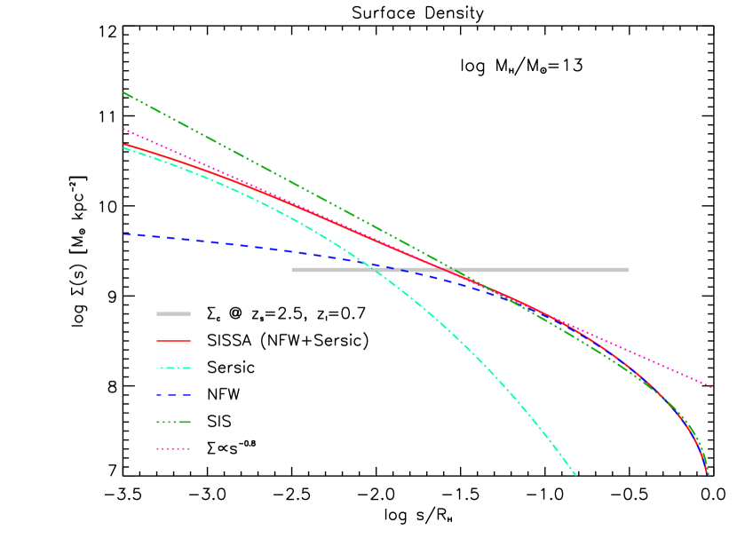
Figure 1.— Surface mass density of an early-type lens. (Blue) dashed line: NFW dark matter profile with $M_{\rm H}=10^{13}\,M_{\odot}$ and concentration parameter $c=5$; (cyan) dot-dashed line: Sérsic profile ($n=4$) of the stellar component in the proportion $M_{\rm H}/M_{\star}=30$; (red) solid line: SISSA model constituted by the sum of the two contributions; (green) triple-dot-dashed line: classical SIS model for the same DM mass; (magenta) dotted line: power law relation $\Sigma(s)\propto s^{-0.8}$, that provides a good approximation to the SISSA model in the radial range relevant for strong gravitational lensing (see text for details). The horizontal grey line represents the critical density for lensing for a source redshift $z_{s}=2.5$ and a lens redshift $z_{\ell}=0.7$. The projected radius $s$ is normalized to the halo virial radius.

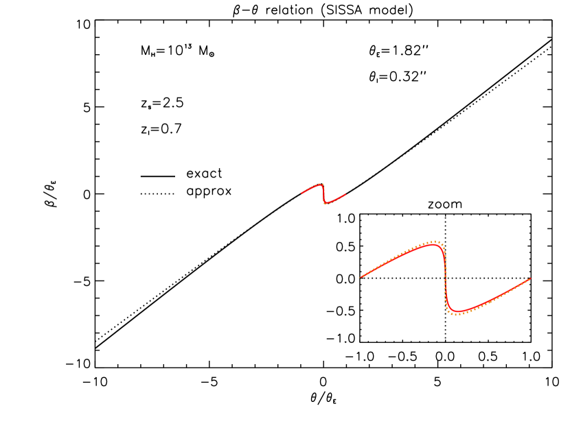
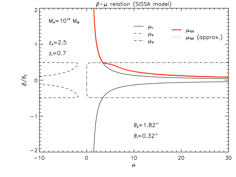
Figure 2.— Solutions of the lens equation for the SISSA model. Top panel: relation between the angular positions of the source $\beta$ and of the images $\theta$, normalized to the position $\theta_{E}$ of the Einstein ring (the red portion of the curve is zoomed in the inset). Bottom panel: relation between the angular position of the source $\beta$ and the amplification $\mu_{\rm i}$ of the three images (the black solid, dashed and dot-dashed curves refer to different images). The red solid curve is the total magnification. In this example, the source is at $z_{s}=2.5$ and the lens at $z_{\ell}=0.7$. The parameters of the lens mass distribution are the same as in Fig. 1. The Einstein ring is located at $\theta_{E}\approx 1.82^{\prime\prime}$. Note that the SISSA and NFW models (but not the SIS model) also feature an inner critical curve at $\theta_{I}\approx 0.32^{\prime\prime}$. In both panels the orange dotted curves show the results obtained using the approximate solutions presented in § 2.3; the agreement with numerical solutions is strikingly good.

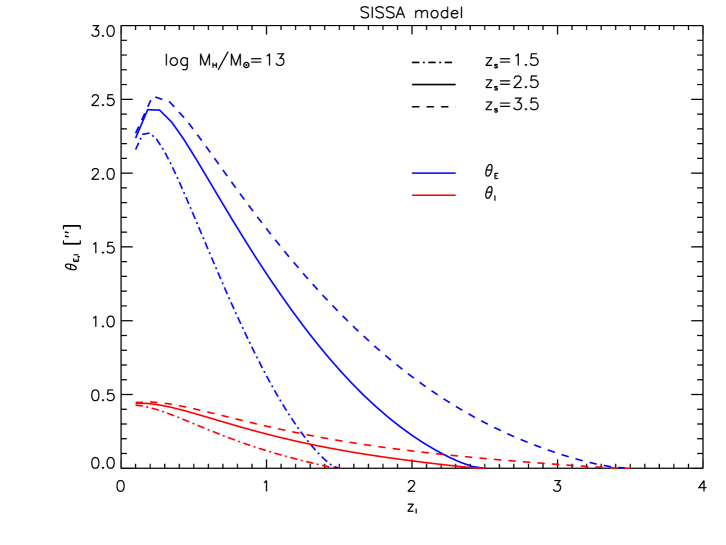
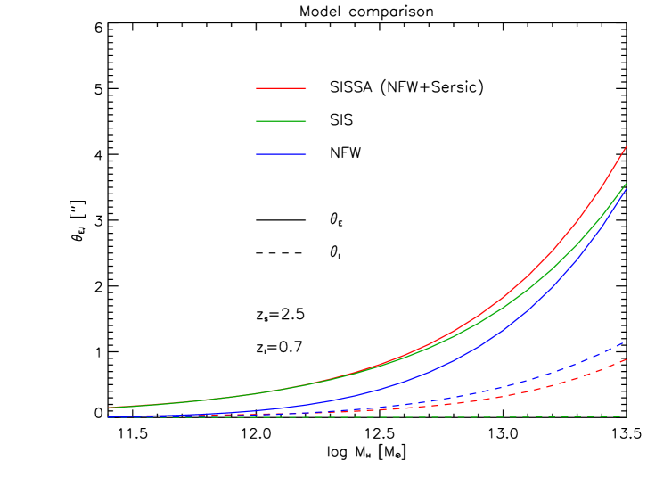
Figure 3.— Top panel: angular positions of the Einstein ring $\theta_{E}$ (blue lines) and of the inner critical curve $\theta_{I}$ (red lines) for the SISSA model, as a function of the lens redshift $z_{\ell}$ and for different source redshifts: $z_{s}=1.5$ (dot-dashed lines); $2.5$ (solid lines); and $3.5$ (dashed lines). The parameters of the lens mass distribution are the same as in Fig. 1. Bottom panel: angular positions of the Einstein ring $\theta_{E}$ (solid lines) and of the inner critical curve $\theta_{I}$ (dashed lines) as a function of the lens mass, for the SISSA (red lines), NFW (blue lines), and SIS (green lines) models. The source is at redshift $z_{s}=2.5$, the lens at $z_{\ell}=0.7$.

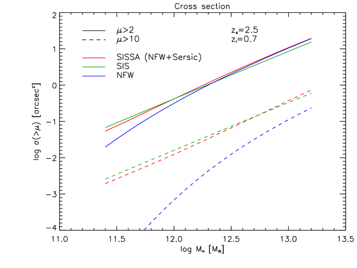
Figure 4.— Lens cross section as a function of the lens mass, for two different amplification thresholds ($\mu>2$, solid lines, and $\mu>10$, dashed lines), and for the SISSA (red lines), NFW (blue lines), and SIS (green lines) models. The source and the lens are at the same redshifts as in Fig. 3.

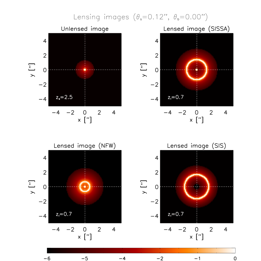
Figure 5.— Ray-tracing simulation of the gravitational lensing for an extended source at $z_{s}=2.5$ with a Sérsic profile ($n=4$) and effective (half light) angular radius $\theta_{s}=0.12^{\prime\prime}$, and a lens at $z_{\ell}=0.7$. The lens parameters are the same as in Fig. 1. The impact parameter $\theta_{b}$ (i.e. the angular separation between the source and the optical axis) is null in this example. The unlensed source is shown in the top left panel, while the lensed image for the SISSA model is in the top right panel, for the NFW model in the bottom left panel, and for the SIS model in the bottom right panel. In all panels the origin of coordinates marks the position of the optical axis, while the color scale represents in logarithmic units the surface brightness relative to the central value of the unlensed image. Note that the central pixels in the SISSA and NFW panels correspond to the strongly demagnified image, and appear in the figure owing to the finite resolution of the simulations.

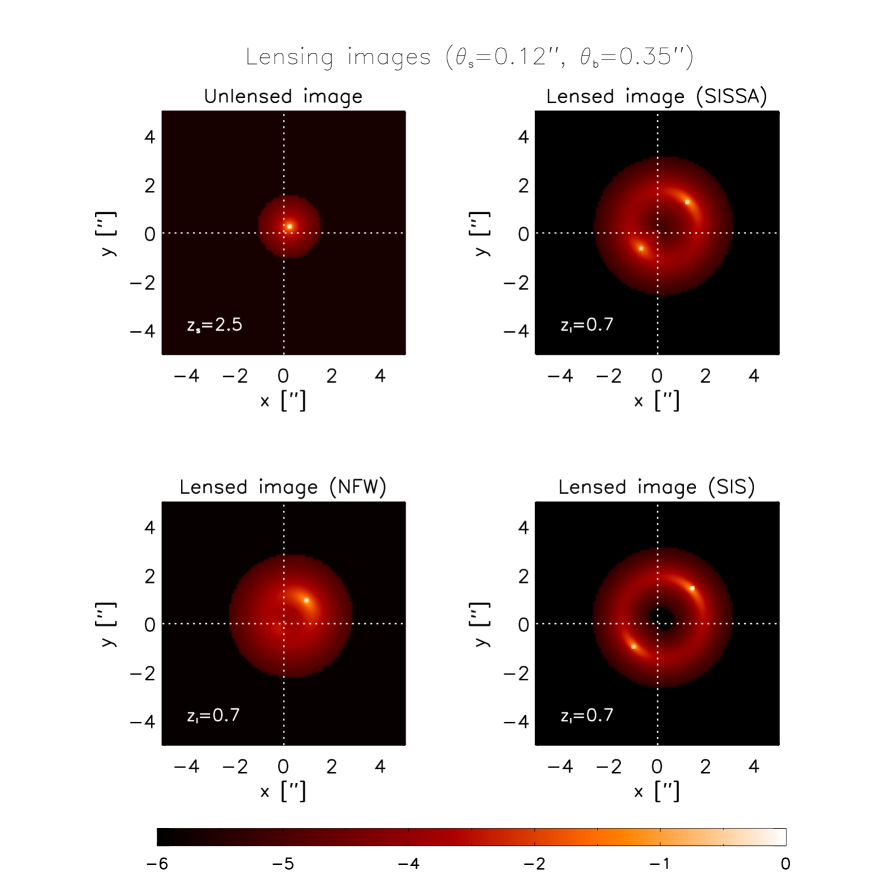
Figure 6.— As in the previous figure, but for an impact parameter $\theta_{b}=0.35^{\prime\prime}$.

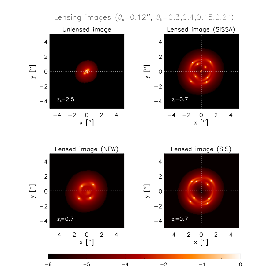
Figure 7.— As in the previous figures, but for four bright spots with impact parameters $\theta_{b}=0.3,0.4,0.15,0.2^{\prime\prime}$, respectively.

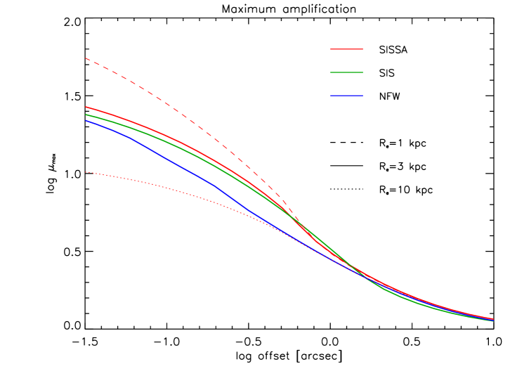
Figure 8.— Maximum amplification for an extended source as a function of the offset between the center of the source and the optical axis, for the SISSA (red line), NFW (blue), and SIS (green) models. The lens parameters and the source redshift are the same as in Fig. 1. The source surface brightness profile is described by a Sérsic law with $n=4$ and effective radius $R_{e}=3$ kpc (solid lines). For the SISSA model we also show the results with $R_{e}=1$ kpc (dashed line) and $R_{e}=10$ kpc (dotted line).

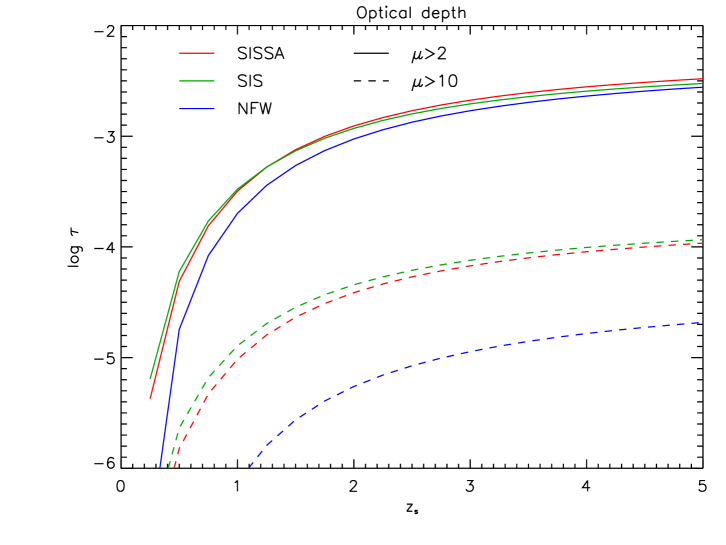
Figure 9.— Lensing optical depth as a function of the source redshift, for two different amplificationx thresholds ($\mu>2$, solid lines and $\mu>10$, dashed lines), and for the SISSA (red lines), NFW (blue lines), and SIS (green lines) models.

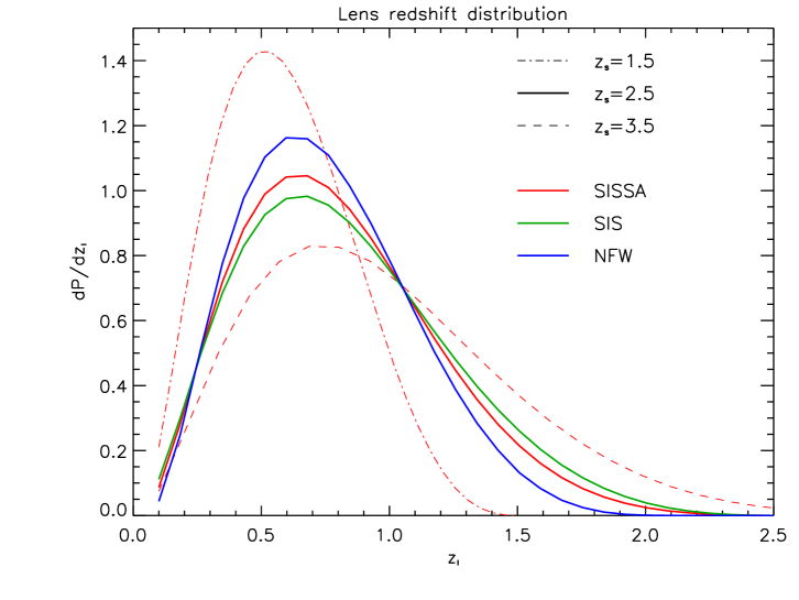
Figure 10.— Lens redshift distributions yielded by the SISSA (red lines), NFW (blue line), and SIS (green line) models for a source redshift $z_{s}=2.5$ (solid lines). For the SISSA model we also show the results for $z_{s}=1.5$ (dot-dashed line) and $z_{s}=3.5$ (dashed line).

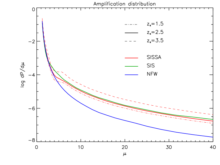
Figure 11.— Amplification distributions yielded by the SISSA (red lines), NFW (blue line), and SIS (green line) models for $z_{s}=2.5$ (solid lines). For the SISSA model we also show the results for $z_{s}=1.5$ (dot-dashed line) and $z_{s}=3.5$ (dashed line).

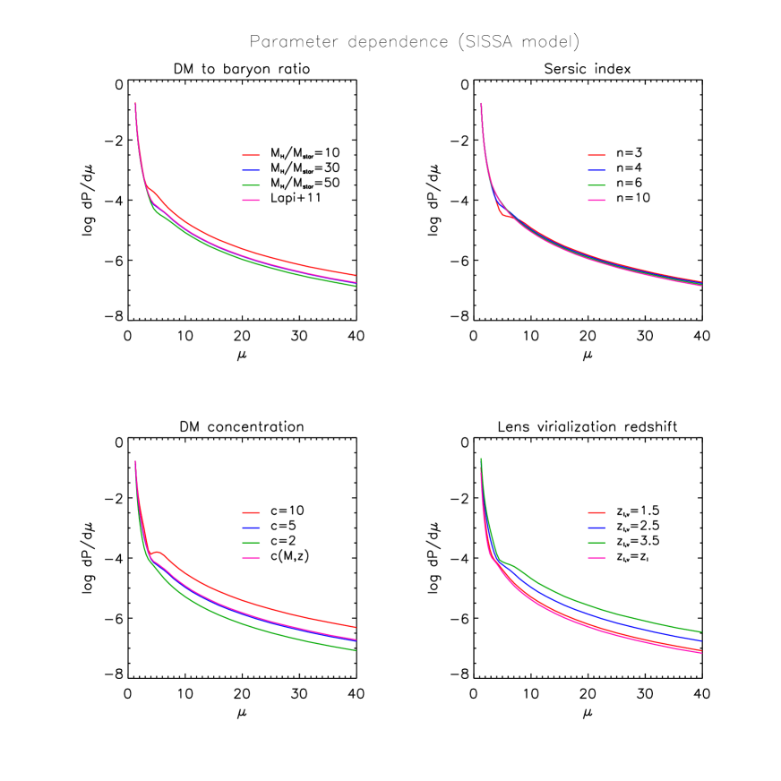
Figure 12.— Dependence of the amplification distribution for the SISSA model on various parameters: DM to stellar mass ratio $M_{\rm H}/M_{\star}$ (top left panel); Sérsic index $n$ (top right panel); DM concentration $c$ (bottom left panel), and lens virialization redshift $z_{\ell,v}$ (bottom right panel).

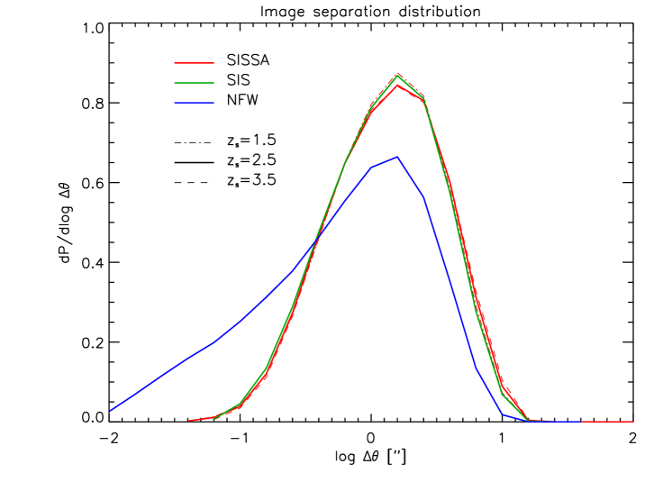
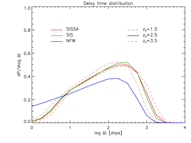
Figure 13.— Top panel: distribution of the separations of the two brightest images of a source at $z_{s}=2.5$ for the SISSA (red lines), NFW (blue line), and SIS (green line) models. For the SISSA models we also show the results for $z_{s}=1.5$ (dot-dashed line) and $z_{s}=3.5$ (dashed line). Bottom panel: delay time distribution; linestyles are as above.

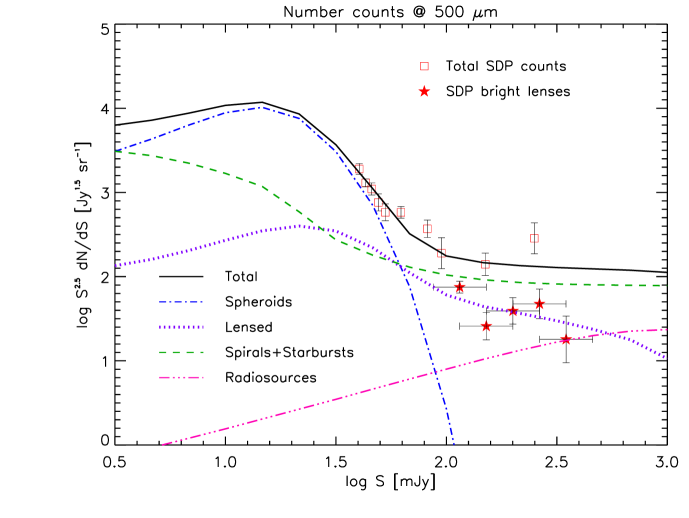
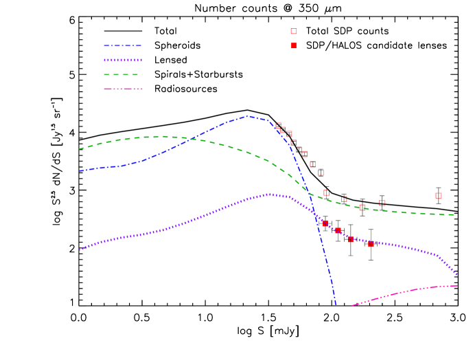
Figure 14.— Top panel: Euclidean normalized counts at $500\,\mu$m. The open squares and the filled stars represent the total Herschel-ATLAS SDP counts (Clements et al. 2010) and the counts of the bright SDP lenses spectroscopically confirmed by Negrello et al. (2010), respectively. The solid line illustrates the total model counts comprising the contributions of unlensed (blue dot-dashed line; Lapi et al. 2011) and strongly lensed (purple dotted line; SISSA model from the present work) proto-spheroidal galaxies, normal late-type plus starburst galaxies (green dashed line; Negrello et al. 2007), radio sources (magenta triple-dot-dashed line; De Zotti et al. 2005). Bottom panel: same but at $350\,\mu$m. Here the filled squares refer to counts of the SDP candidate lenses selected by Gonzalez-Nuevo et al. (2012).

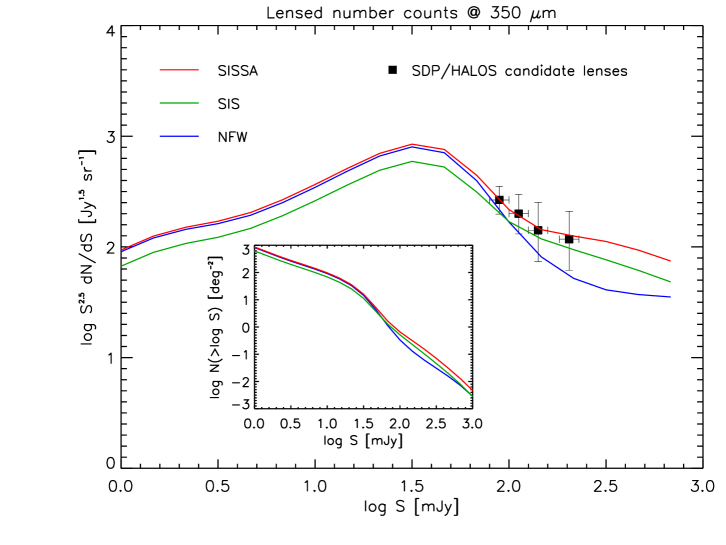
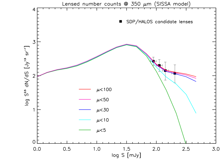
Figure 15.— Top panel: Euclidean normalized counts of lensed galaxies at $350\,\mu$m. The filled squares refer to the SDP candidate strongly lensed galaxies selected by Gonzalez-Nuevo et al. (2012). Our model predictions are also plotted, for the SISSA (red lines), NFW (blue lines), and SIS (green lines) models. In the inset the corresponding integral counts are plotted. Bottom panel: same as above, but for the SISSA model with different cuts in maximum amplification: $\mu_{\rm max}=5$, 10, 30, 50, and 100 (green, cyan, blue, magenta, and red line, respectively). The line with $\mu_{\rm max}=100$ is indistinguishable from that without amplification cut.

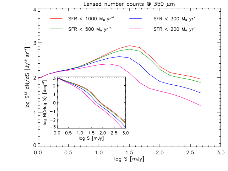
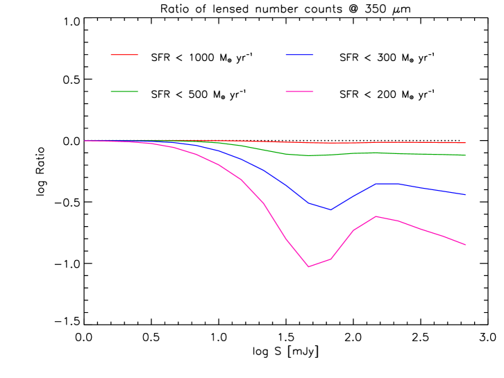
Figure 16.— Top panel: Euclidean normalized counts of lensed galaxies at $350\,\mu$m. Our model predictions on the counts of lensed proto-spheroidal galaxies for the SISSA model are plotted for different upper limits to the star formation rate: SFR $\leq 200$, $300$, $500$, and $1000\,M_{\odot}$ yr^-1 (magenta, blue, green, and red lines, respectively); the latter line is undistinguishable from that without SFR limit. In the inset the corresponding integral counts are plotted. Bottom panel: ratio between the counts of lensed galaxies with SFRs below the above thresholds and those without any SFR limit.

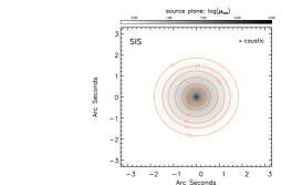
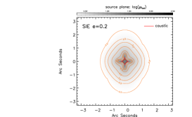
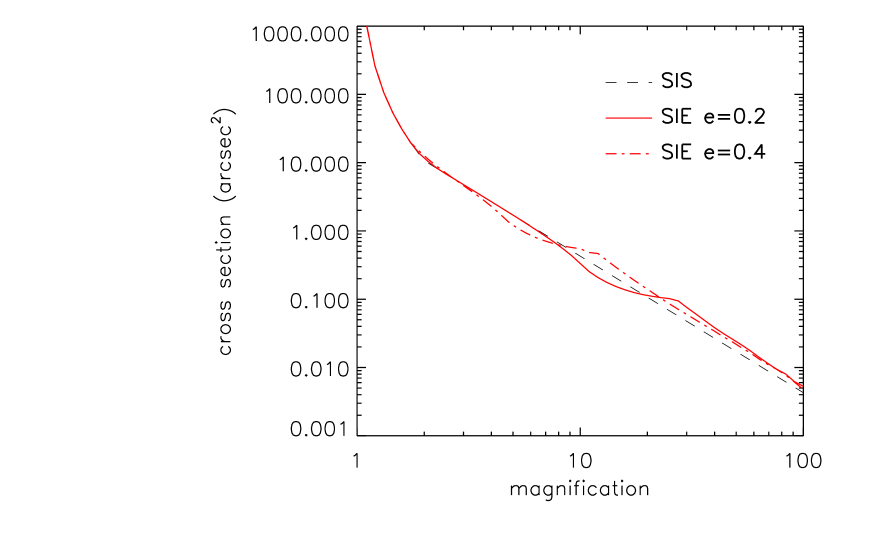
Figure 17.— Top panels: map of the total amplification as a function of the source position from the center of the lensing mass, for a SIS lens (left), and for a SIE lens with ellipticity $\mathrm{e}=0.2$ (middle) and $\mathrm{e}=0.4$ (right). The lens and the source are assumed to be at redshift $0.7$ and $2.5$, respectively. The orange lines represent contours of equal amplifications ranging from $2$ to $10$, while the red point/curve mark the caustics. Bottom panel: corresponding cross sections for lensing as a function of the total amplification for the SIS lens (black dashed line), and for the SIE lens with $\mathrm{e}=0.2$ (red solid line) and $\mathrm{e}=0.4$ (red dot-dashed line).

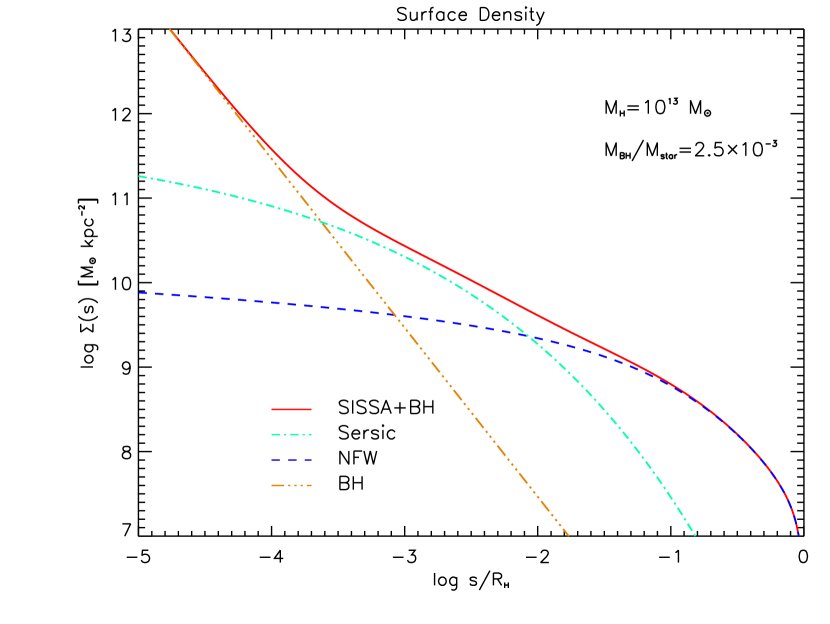
Figure 18.— Surface density profile of a configuration constituted by an early-type galaxies and a central super-massive BH. This figure should be contrasted with Fig. 1 which represents the same configuration without central super-massive BH. (Blue) dashed line: dark matter component with mass $M_{\rm H}=10^{13}\,M_{\odot}$ and NFW profile with concentration parameter $c=5$. (Cyan) dot-dashed line: stellar component in the proportion $M_{\rm H}/M_{\star}=30$ relative to the DM with a Sérsic $n=4$ profile. (Orange) triple-dot-dashed line: super-massive BH with mass ratio $M_{\bullet}/M_{\star}=2.5\times 10^{-3}$. (Red) solid line: SISSA$+$BH model, sum of the three contributions. Note that here, to avoid representing the central singularity, we rendered the point mass surface density with the powerlaw $\Sigma(\theta)\propto\theta^{-\eta}$ in the limit $\eta\rightarrow 2$ (see § 5.4).

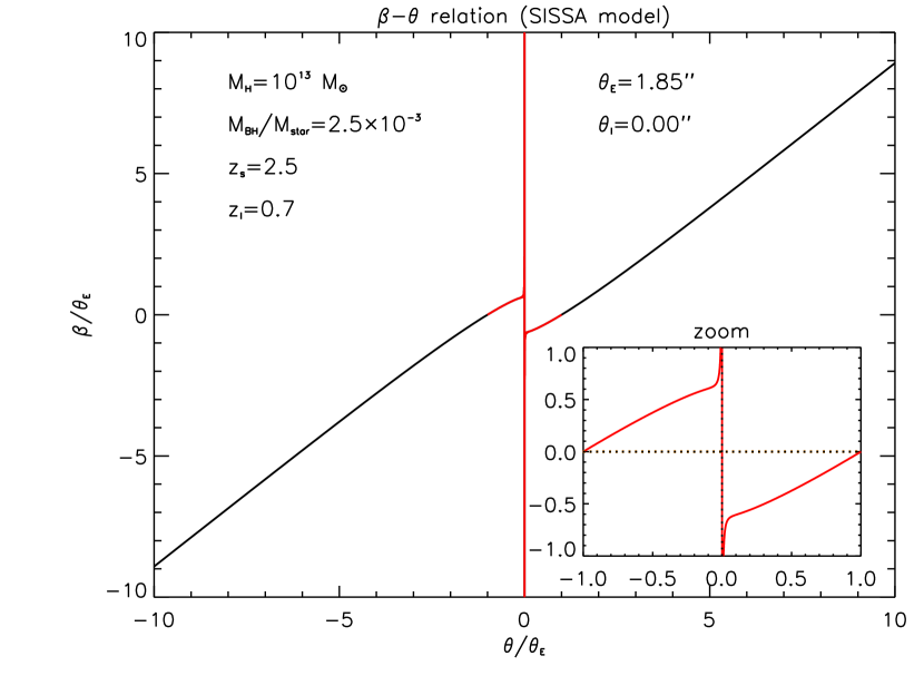
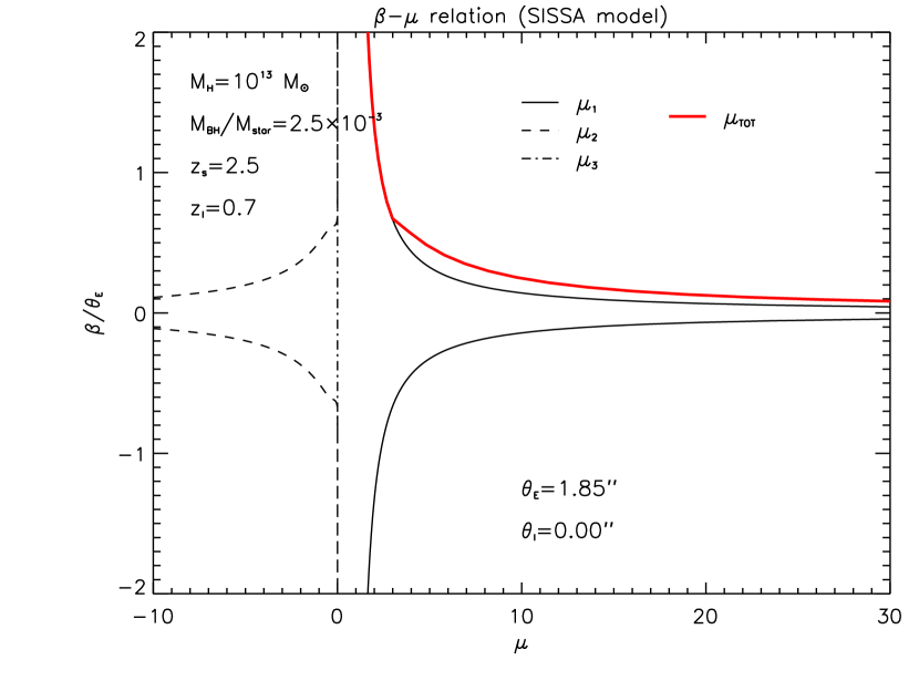
Figure 19.— Solutions of the lensing equation for the SISSA model, including a central super-massive BH with mass ratio $M_{\bullet}/M_{\star}=2.5\times 10^{-3}$. This figure should be contrasted with Fig. 2, which corresponds to the same configuration without central super-massive BH. Linestyles as in Fig. 2.

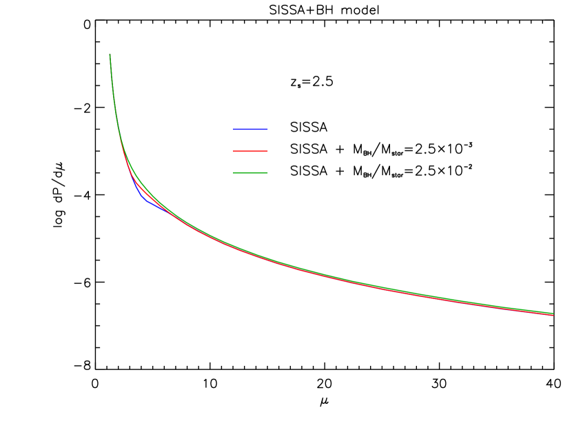
Figure 20.— Differential amplification distribution for a configuration constituted by an early-type galaxies and a central super-massive BH. Blue line: SISSA model with fiducial parameter values, without central super-massive BH. Red line: SISSA model plus a super-massive BH with standard mass ratio $M_{\bullet}/M_{\star}=2.5\times 10^{-3}$. Green line: SISSA model plus a super-massive BH with a high mass ratio $M_{\bullet}/M_{\star}=2.5\times 10^{-2}$.

Table 1Power law fits of the surface density profile

Lens parameter						$M_{\rm H}=10^{13}\,M_{\odot}$				$M_{\rm H}=10^{12}\,M_{\odot}$				$M_{\rm H}=10^{11}\,M_{\odot}$
$M_{\rm H}/M_{\star}$		$n$		$c$		$\log\Sigma_{0}$		$\eta$		$\log\Sigma_{0}$		$\eta$		$\log\Sigma_{0}$		$\eta$
$30$		$4$		$5$		$9.621$		$0.823$		$9.326$		$0.871$		$9.013$		$0.902$
$10$		$4$		$5$		$9.780$		$0.936$		$9.537$		$1.036$		$9.275$		$1.124$
$50$		$4$		$5$		$9.561$		$0.773$		$9.249$		$0.801$		$8.922$		$0.814$
$70$		$4$		$5$		$9.528$		$0.743$		$9.208$		$0.761$		$8.874$		$0.765$
L+11		$4$		$5$		$9.610$		$0.815$		$9.351$		$0.893$		$9.095$		$0.977$
$30$		$3$		$5$		$9.629$		$0.828$		$9.348$		$0.892$		$9.042$		$0.934$
$30$		$6$		$5$		$9.604$		$0.811$		$9.295$		$0.841$		$8.975$		$0.861$
$30$		$10$		$5$		$9.578$		$0.789$		$9.258$		$0.806$		$8.932$		$0.816$
$30$		$4$		$2$		$9.472$		$0.793$		$9.189$		$0.855$		$8.882$		$0.895$
$30$		$4$		$10$		$9.912$		$0.982$		$9.601$		$1.011$		$9.280$		$1.030$
$30$		$4$		$c(M)$		$9.621$		$0.823$		$9.369$		$0.886$		$9.101$		$0.932$

Note. — Power law fits of the surface density profile [Eq. (9) over the radial range $10^{-2.5}\lesssim s/R_{\rm H}\lesssim 10^{-1}$ for halo masses $M_{\rm H}=10^{11}$, $10^{12}$, and $10^{13}\,M_{\odot}$. The normalization $\Sigma_{0}$ (in $M_{\odot}$ kpc^-2) refers to a projected radius $s_{0}=10^{-2}\,R_{\rm H}$. The table shows the dependence of the fits on the parameters of the lens mass distribution, namely, dark matter to star mass ratio $M_{\rm H}/M_{\star}$, Sérsic index $n$, and halo concentration $c$. The case L+11 takes into account the dependence of ratio $M_{\rm H}/M_{\star}$ on $M_{\rm H}$ as implied by the Lapi et al. (2011) model.

References

- (1)
- (2) Abadi, M. G., Navarro, J. F., Fardal, M., Babul, A., & Steinmetz, M. 2010, MNRAS, 407, 435
- (3)
- (4) Auger, M. W., Treu, T., Bolton, A. S., et al. 2009, ApJ, 705, 1099
- (5)
- (6) Baldry, I. K., Glazebrook, K., Brinkmann, J., et al. 2004, ApJ, 600, 681
- (7)
- (8) Barkana, R., & Loeb, A. 2001, Phys. Rep., 349, 125
- (9)
- (10) Barnabè, M., Czoske, O., Koopmans, L. V. E., Treu, T., & Bolton, A. S. 2011, MNRAS, 415, 2215
- (11)
- (12) Belokurov, V., Evans, N. W., Moiseev, A., et al. 2007, ApJ, 671, L9
- (13)
- (14) Bernardi, M., Shankar, F., Hyde, J. B., et al. 2010, MNRAS, 404, 2087
- (15)
- (16) Blain, A. W. 1996, MNRAS, 283, 1340
- (17)
- (18) Blumenthal, G. R., Faber, S. M., Flores, R., & Primack, J. R. 1986, ApJ, 301, 27
- (19)
- (20) Bolton, A. S., Burles, S., Koopmans, L. V. E., Treu, T., & Moustakas, L. A. 2006, ApJ, 638, 703
- (21)
- (22) Bolton, A. S., Burles, S., Koopmans, L. V. E., et al. 2008, ApJ, 682, 964
- (23)
- (24) Bolton, A. S., Brownstein, J. R., Kochanek, C. S., et al. 2012, ApJ, submitted [preprint arXiv:1201.2988]
- (25)
- (26) Browne, I. W. A., Wilkinson, P. N., Jackson, N. J. F., et al. 2003, MNRAS, 341, 13
- (27)
- (28) Brownstein, J. R., Bolton, A. S., Schlegel, D. J., et al. 2012, ApJ, 744, 41
- (29)
- (30) Bryan, G. L., & Norman, M. L. 1998, ApJ, 495, 80
- (31)
- (32) Cabanac, R. A., Alard, C., Dantel-Fort, M., et al. 2007, A&A, 461, 813
- (33)
- (34) Churazov, E., Tremaine, S., Forman, W., et al. 2010, MNRAS, 404, 1165
- (35)
- (36) Cimatti, A., Cassata, P., Pozzetti, L., et al. 2008, A&A, 482, 21
- (37)
- (38) Cirasuolo, M., Shankar, F., Granato, G. L., De Zotti, G., & Danese, L. 2005, ApJ, 629, 816
- (39)
- (40) Clements, D. L., Rigby, E., Maddox, S., et al. 2010, A&A, 518, L8
- (41)
- (42) El-Zant, A., Shlosman, I., & Hoffman, Y. 2001, ApJ, 560, 636
- (43)
- (44) de Vaucouleurs, G. 1948, Ann. Astroph., 11, 247
- (45)
- (46) de Zotti, G., Ricci, R., Mesa, D., et al. 2005, A&A, 431, 893
- (47)
- (48) Eales, S., Dunne, L., Clements, D., et al. 2010, PASP, 122, 499
- (49)
- (50) Fan, L., Lapi, A., Bressan, A., et al. 2010, ApJ, 718, 1460
- (51)
- (52) Faure, C., Kneib, J.-P., Covone, G., et al. 2008, ApJS, 176, 19
- (53)
- (54) Ferrarese, L., & Ford, H. 2005, Space Sci. Rev., 116, 523
- (55)
- (56) Förster Schreiber, N. M., Genzel, R., Lehnert, M. D., et al. 2006, ApJ, 645, 1062
- (57)
- (58) Förster Schreiber, N. M., Shapley, A. E., Genzel, R., et al. 2011, ApJ, 739, 45
- (59)
- (60) Genzel, R., Tacconi, L. J., Eisenhauer, F., et al. 2006, Nature, 442, 786
- (61)
- (62) Gerhard, O., Kronawitter, A., Saglia, R. P., & Bender, R. 2001, AJ, 121, 1936
- (63)
- (64) Gnedin, O. Y., Ceverino, D., Gnedin, N. Y., et al. 2012, ApJ, submitted [preprint arXiv:1108.5736]
- (65)
- (66) Gnedin, O Y., Kravtsov, A. V., Klypin, A. A., & Nagai, D. 2004, ApJ, 616, 16
- (67)
- (68) González-Nuevo, J., Lapi, A., Fleuren, S., et al. 2012, arXiv:1202.0402
- (69)
- (70) Granato, G. L., De Zotti, G., Silva, L., Bressan, A., & Danese, L. 2004, ApJ, 600, 580
- (71)
- (72) Grillo, C. 2012, ApJ, 747, L15
- (73)
- (74) Grillo, C., Lombardi, M., & Bertin, G. 2008, A&A, 477, 397
- (75)
- (76) Humphrey, P. J., & Buote, D. A. 2010, MNRAS, 403, 2143
- (77)
- (78) Hyde, J. B., & Bernardi, M. 2009, MNRAS, 396, 1171
- (79)
- (80) Jain, B. & Lima, M. 2011, MNRAS, 411, 2113
- (81)
- (82) Kleinheinrich, M., Rix, H.-W., Erben, T., et al. 2005, A&A, 439, 513
- (83)
- (84) Kochanek, C. S. 2006, in ‘Gravitational lensing: strong, weak and micro’, eds. G. Meylan, P. Jetzer and P. North (Berlin: Springer), p. 91
- (85)
- (86) Kochanek, C. S., & White, M. 2001, ApJ, 559, 531
- (87)
- (88) Komatsu, E., Smith, K. M., Dunkley, J., et al. 2011, ApJS, 192, 18
- (89)
- (90) Koopmans, L. V. E., Bolton, A., Treu, T., et al. 2009, ApJ, 703, L51
- (91)
- (92) Koopmans, L. V. E., Browne, I. W. A., & Jackson, N. J. 2004, NewAR, 48, 1085
- (93)
- (94) Kormendy, J., Fisher, D. B., Cornell, M. E., & Bender, R. 2009, ApJS, 182, 216
- (95)
- (96) Kronawitter, A., Saglia, R. P., Gerhard, O., & Bender, R. 2000, A&AS, 144, 53
- (97)
- (98) Kubo J. M., Dell’Antonio I. P., 2008, MNRAS, 385, 918
- (99)
- (100) Lagattuta, D. J., Fassnacht, C. D., Auger, M. W., et al. 2010, ApJ, 716, 1579
- (101)
- (102) Lapi, A., González-Nuevo, J., Fan, L., et al. 2011, ApJ, 742, 24
- (103)
- (104) Lapi, A., Shankar, F., Mao, J., et al. 2006, ApJ, 650, 42
- (105)
- (106) Li, L.-X., & Ostriker, J. P. 2003, ApJ, 595, 603
- (107)
- (108) Łokas, E. L., & Mamon, G. A. 2001, MNRAS, 321, 155
- (109)
- (110) Magliocchetti, M., & Porciani, C. 2003, MNRAS, 346, 186
- (111)
- (112) Maier, C., Lilly, S. J., Zamorani, G., et al. 2009, ApJ, 694, 10
- (113)
- (114) Mandelbaum, R., Seljak, U., Kauffmann, G., et al. 2006, MNRAS, 368, 715
- (115)
- (116) Mao, J., Lapi, A., Granato, G. L., de Zotti, G., & Danese, L. 2007, ApJ, 667, 655
- (117)
- (118) McConnell, N.J., Ma, C.-P., Gebhardt, K., et al. 2011, Nature, 480, 215
- (119)
- (120) Mo, H.J., Mao, S., & White, S.D.M. 1998, MNRAS, 295, 319
- (121)
- (122) Moreno, J., et al. 2009, MNRAS, 397, 299
- (123)
- (124) Moster, B. P., Somerville, R. S., Maulbetsch, C., et al. 2010, ApJ, 710, 903
- (125)
- (126) Navarro, J. F., Frenk, C. S., & White, S. D. M. 1996, ApJ, 462, 563
- (127)
- (128) Negrello, M., Hopwood, R., De Zotti, G., et al. 2010, Science, 330, 800
- (129)
- (130) Negrello, M., Perrotta, F., González-Nuevo, J., et al. 2007, MNRAS, 377, 1557
- (131)
- (132) Oguri, M. 2010, PASJ, 62, 1017
- (133)
- (134) Oguri, M., & Marshall, P. J. 2010, MNRAS, 405, 2579
- (135)
- (136) Oguri, M., Taruya, A., Suto, Y., & Turner, E. L. 2002, ApJ, 568, 488
- (137)
- (138) Peacock, J. A. 1982, MNRAS, 199, 987
- (139)
- (140) Pedrosa, S., Tissera, P. B., & Scannapieco, C. 2010, MNRAS, 402, 776
- (141)
- (142) Perrotta, F., Baccigalupi, C., Bartelmann, M., De Zotti, G., & Granato, G. L. 2002, MNRAS, 329, 445
- (143)
- (144) Perrotta, F., Magliocchetti, M., Baccigalupi, C., et al. 2003, MNRAS, 338, 623
- (145)
- (146) Porciani, C., & Madau, P. 2000, ApJ, 532, 679
- (147)
- (148) Prada, F., Klypin, A. A., Cuesta, A. J., Betancort-Rijo, J. E., & Primack, J. 2011, arXiv:1104.5130
- (149)
- (150) Prugniel, P., & Simien, F. 1997, A&A, 321, 111
- (151)
- (152) Ragone-Figueroa, C., Granato, G. L., & Abadi, M. G. 2012, MNRAS, in press [preprint arXiv:1202.1527]
- (153)
- (154) Renzini, A. 2006, ARA&A, 44, 141
- (155)
- (156) Rodionov, S. A., & Athanassoula, E. 2011, MNRAS, 410, 111
- (157)
- (158) Ruff, A. J., Gavazzi, R., Marshall, P. J., et al. 2011, ApJ, 727, 96
- (159)
- (160) Rusin, D., Keeton, C.R., & Winn, J.N. 2005, ApJ, 627, L93
- (161)
- (162) Schneider, P., Ehlers, J., & Falco, E. E. 1992, Gravitational Lenses, XIV, Springer-Verlag Berlin Heidelberg New York
- (163)
- (164) Serjeant, S. 2011, in ‘The Spectral Energy Distribution of Galaxies’, eds. R.J. Tuffs and C.C. Popescu, in press [preprint arXiv:1112.0323]
- (165)
- (166) Shankar, F., Lapi, A., Salucci, P., De Zotti, G., & Danese, L. 2006, ApJ, 643, 14
- (167)
- (168) Shen, S., Mo, H. J., White, S. D. M., et al. 2003, MNRAS, 343, 978
- (169)
- (170) Sheth, R. K., & Tormen, G. 1999, MNRAS, 308, 119
- (171)
- (172) Sheth, R. K., & Tormen, G. 2002, MNRAS, 329, 61
- (173)
- (174) Spiniello, C., Koopmans, L. V. E., Trager, S. C., Czoske, O., & Treu, T. 2011, MNRAS, 417, 3000
- (175)
- (176) Swinbank, A. M., Smail, I., Longmore, S., et al. 2010, Nature, 464, 733
- (177)
- (178) Thomas, J., Saglia, R. P., Bender, R., et al. 2011, MNRAS, 415, 545
- (179)
- (180) Tonini, C., Lapi, A., & Salucci, P. 2006a, ApJ, 649, 591
- (181)
- (182) Tonini, C., Lapi, A., & Salucci, P. 2006b, ApJ, 638, L13
- (183)
- (184) Treu, T., Dutton, A. A., Auger, M. W., et al. 2011, MNRAS, 417, 1601
- (185)
- (186) Vale, A., & Ostriker, J. P. 2004, MNRAS, 353, 189
- (187)
- (188) Vale, A., & Ostriker, J. P. 2006, MNRAS, 371, 1173
- (189)
- (190) van den Bosch, F. C., Tormen, G., & Giocoli, C. 2005, MNRAS, 359, 1029
- (191)
- (192) Vieira, J. D., Crawford, T. M., Switzer, E. R., et al. 2010, ApJ, 719, 763
- (193)
- (194) Weijmans, A.-M., Krajnović, D., van de Ven, G., et al. 2008, MNRAS, 383, 1343
- (195)
- (196) Willis, J. P., Hewett, P. C., Warren, S. J., Dye, S., & Maddox, N. 2006, MNRAS, 369, 1521
- (197)