Transceiver Design for Multi-user Multi-
antenna Two-way Relay Cellular Systems

Abstract

In this paper, we design interference free transceivers for multi-user two-way relay systems, where a multi-antenna base station (BS) simultaneously exchanges information with multiple single-antenna users via a multi-antenna amplify-and-forward relay station (RS). To offer a performance benchmark and provide useful insight into the transceiver structure, we employ alternating optimization to find optimal transceivers at the BS and RS that maximizes the bidirectional sum rate. We then propose a low complexity scheme, where the BS transceiver is the zero-forcing precoder and detector, and the RS transceiver is designed to balance the uplink and downlink sum rates. Simulation results demonstrate that the proposed scheme is superior to the existing zero forcing and signal alignment schemes, and the performance gap between the proposed scheme and the alternating optimization is minor.

I Introduction

Two-way relay (TWR) techniques have attracted considerable interest owing to its high spectral efficiency. Most of prior works study TWR systems with single user pair, where two users exchange information via a single relay station (RS) [1, 2, 3]. Various transmission schemes have been proposed for single antenna nodes [1] and multi-antenna nodes [2, 3].

Recently, the design for TWR systems is extended to multi-user cases [4, 5, 6, 7, 8, 9, 10, 11], which can be roughly divided into two categories based on the system topologies, i.e., symmetric and asymmetric systems. In symmetric systems [4, 5, 6], multiple user pairs exchange information via a RS. In asymmetric systems, a base station (BS) exchanges messages with multiple users [7, 8, 11, 9, 10], which is a typical scenario of cellular networks.

In this paper, we study multi-user TWR cellular system, where a multi-antenna BS communicates with multiple single-antenna users bidirectionally via a multi-antenna amplify-and-forward (AF) relay. Owing to the importance from practical perspective, there is a considerable amount of work on designing transceivers for such a system [8, 11, 9, 10]. However, its transceiver optimization is challenging due to the complicated interference among multiple users in the broadcast and multi-access phases, and even its bidirectional sum capacity is still not available until now.

Allocating orthogonal time or frequency resources to the uplink and downlink signals of different users is an immediate way to eliminate the interference [7], with which existing single-user TWR techniques can be directly applied. Since this is far from optimal, a further attempt is to introduce an interference free constraint, which is essentially the zero-forcing (ZF) principle. Though also suboptimal in a sense of sum rate, such a design can capture the inherent degrees of freedom of the system, which is an approximate characterization of the capacity at the high signal-to-noise (SNR) level. Along this line, several ZF-principle based transceivers have been proposed. Considering that the RS is equipped with multiple antennas, a natural solution is to apply ZF transceiver at the RS to separate all the signals from and to the BS and users [8]. This ZF scheme employs orthogonal spatial resources to differentiate different links, thereby the RS should be equipped with enough antennas. To remove all the interference, at least $2N$ antennas are required at the RS for a system with $N$ antennas at the BS and $N$ single antenna users. When the RS is only with $N$ antennas, the multiple antennas at the BS also need to be exploited to ensure interference free transmission. In [9, 10, 11], the concept of signal alignment (SA) [12] is employed to reduce the number of interference experienced at the relay. The SA scheme exploits the self-interference cancelation (SIC) [13] ability of TWR. Its basic idea is to project the uplink and downlink signals of each user onto the same spatial direction at the RS through proper BS precoding, such that the RS can separate $N$ superimposed signals. After receiving a superimposed signal forwarded by the RS, each user removes its transmitted uplink signal via SIC, and obtains its desired downlink signal.

Both the ZF and SA schemes are based on ZF-principle. Nonetheless, they are not the only interference free solution. In fact, by analyzing the feasibility of interference free constraints for multi-user multi-antenna TWR cellular systems, it is not hard to show that the SA scheme is the unique solution only for special antenna configurations, and the ZF scheme ensures interference free transmission only when the number of antennas at the RS is sufficiently large. Moreover, both of them are designed as low complexity schemes without taking into account the sum rate.

In this paper, we strive to find a low complexity interference free transceiver towards maximizing sum rate under general antenna settings. To provide a performance benchmark as well as useful insight into the transceiver structure, we employ a standard alternating optimization technique [14] to optimize the BS and RS transceivers aiming at maximizing bidirectional sum rate under interference free constraints. In order to develop a low complexity transceiver scheme, we fix the BS transceiver as the optimal BS precoder and detector in high power region found from the alternating optimization. Based on which we first optimize the RS transceiver to separately maximize the uplink and downlink sum rates and then balance the uplink and downlink sum rates to maximize the bidirectional sum rate. Simulation results show that the balanced scheme performs very close to the alternating optimization solution, and outperforms existing ZF and SA schemes under various scenarios.

The rest of the paper is organized as follows. Section II describes the system model. Section III introduces the alternating optimization solution. The balanced transceiver scheme is proposed in IV. Simulation results are given in section V, and conclusions are drawn in section VI. The major symbols used in the paper are summarized in Table I.

TABLE I: List of important symbols

$N_{B}$, $N_{R}$, $N_{U}$	BS or RS antenna number or user number
$\mathbf{H}_{br},\mathbf{H}_{ur}$	Channel matrix from the BS or from all users to the RS
$\mathbf{h}_{ir}$	Channel vector from the $i$th user to the RS
$\overline{\mathbf{H}}_{ir}$	Channel matrix from all users other than the $i$th user to the RS.
	It is obtained from $\mathbf{H}_{ur}$ with the $i$th column, $\mathbf{h}_{ir}$, being removed.
$\mathbf{W}_{bt}$, $\mathbf{W}_{br}$	BS transmit or receive weighting matrix
$\mathbf{w}_{bti}$, $\mathbf{w}_{bri}$	The $i$th column of $\mathbf{W}_{bt}$ or $\mathbf{W}_{br}$
$\mathbf{W}_{r}$	RS weighting matrix
$\mathbf{x}_{b}$	Downlink signal vector transmitted by the BS
$\mathbf{x}_{u}$	Uplink signal vector transmitted by all users
$\mathbf{y}_{r}$	RS’s received signal vector in first phase
$\mathbf{y}_{b},y_{ui}$	BS’s or the $i$th user’s received signal in second phase
$P_{B}$, $P_{R}$, $P_{U}$	The transmit power of BS or RS or a single user
$N_{0}$	Noise variance
$R_{U}$, $R_{D}$, $R_{S}$	Uplink or downlink or bidirectional sum rate
$\mathbf{I}_{N}$	Identity matrix of size $N$
$(\cdot)^{T}$, $(\cdot)^{H}$, $(\cdot)^{*}$	Transpose, conjugate transpose or conjugate of a matrix
$\lVert\cdot\rVert$, $(\cdot)^{\dagger}$	Norm or pseudo inverse of a matrix
$S_{\bot}(\mathbf{X})$	Orthogonal subspace of matrix $\mathbf{X}$
	$S_{\bot}(\mathbf{X})=\mathbf{I}-\mathbf{X}^{H}(\mathbf{X}\mathbf{X}^{H})^{-1}\mathbf{X}$ if $\mathbf{X}$ is a wide matrix
	$S_{\bot}(\mathbf{X})=\mathbf{I}-\mathbf{X}(\mathbf{X}^{H}\mathbf{X})^{-1}\mathbf{X}^{H}$ if $\mathbf{X}$ is a high matrix
$\text{diag}(\mathbf{m})$	Diagonal matrix whose diagonal elements are the elements of vector $\mathbf{m}$
$E(\cdot)$	Mean value of a random variable

II System Model

We consider a multi-user multi-antenna TWR system, which consists of a BS equipped with $N_{B}$ antennas, a RS equipped with $N_{R}$ antennas and $N_{U}$ single-antenna users. The BS and multiple users exchange downlink and uplink information via the RS, as shown in Fig. 1. The bidirectional transmission takes place in two phases.

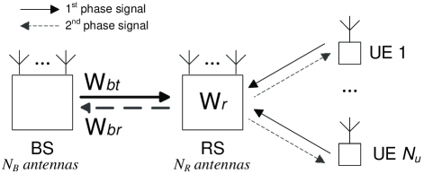
Figure 1: System model of the multi-user multi-antenna TWR cellular system

At the first phase, both the BS and multiple users transmit to the RS. The received signal at the RS is given by

$$\mathbf{y}_{r} =\mathbf{H}_{br}\mathbf{W}_{bt}\mathbf{x}_{b}+\sqrt{P_{U}}\mathbf{H}_{ur}\mathbf{x}_{u}+\mathbf{n}_{r},$$ (1)

where $\mathbf{H}_{br}\in\mathbb{C}^{N_{R}\times N_{B}}$ is the channel matrix from the BS to the RS, $\mathbf{H}_{ur}=(\mathbf{h}_{1r},\cdots,\mathbf{h}_{N_{U}r})$, $\mathbf{h}_{ir}\in\mathbb{C}^{N_{R}\times 1}$ is the channel vector from the $i$th user to the RS, $\mathbf{x}_{b}$ and $\mathbf{x}_{u}$ are the downlink and uplink signal vectors to and from $N_{U}$ users and we assume $E(\mathbf{x}_{b}\mathbf{x}_{b}^{H})=E(\mathbf{x}_{u}\mathbf{x}_{u}^{H})=\mathbf{I}_{N_{U}}$, $P_{U}$ is the transmit power of each user, $\mathbf{n}_{r}$ is the Gaussian noise vector at the RS with zero mean and covariance matrix $N_{0}\mathbf{I}_{N_{R}}$, and $\mathbf{W}_{bt}\in\mathbb{C}^{N_{B}\times N_{U}}$ is the precoder matrix at the BS, which satisfies the transmit power constraint as follows

$$\lVert\mathbf{W}_{bt}\rVert^{2}\leq P_{B},$$ (2)

where $P_{B}$ is the maximal transmit power of the BS.

At the second phase, the RS precodes its received signals and then broadcasts them to the BS and users. The received signals at the BS and the $i$th user are respectively given by

$$\mathbf{y}_{b} =\mathbf{W}_{br}^{T}(\mathbf{H}_{br}^{T}\mathbf{W}_{r}\mathbf{y}_{r}+\mathbf{n}_{b}),$$ (3)

$$y_{ui} =\mathbf{h}_{ir}^{T}\mathbf{W}_{r}\mathbf{y}_{r}+n_{ui},~{}~{}(1\leq i\leq N_{U}),$$ (4)

where $\mathbf{W}_{r}\in\mathbb{C}^{N_{R}\times N_{R}}$ is the weighting matrix at the RS, $\mathbf{W}_{br}\in\mathbb{C}^{N_{B}\times N_{U}}$ is the receive weighting matrix at the BS, and $\mathbf{n}_{b}$ and $n_{ui}$ are Gaussian noises at the BS and the $i$th user, each with zero mean and variance $N_{0}$.

The RS weighting matrix should satisfy the transmit power constraint $E(\lVert\mathbf{W}_{r}\mathbf{y}_{r}\rVert^{2})\leq P_{R}$, which can be rewritten as follows after substituting (1),

$$\lVert\mathbf{W}_{r}\mathbf{H}_{br}\mathbf{W}_{bt}\rVert^{2}+P_{U}\lVert\mathbf{W}_{r}\mathbf{H}_{ur}\rVert^{2}+N_{0}\lVert\mathbf{W}_{r}\rVert^{2}\leq P_{R},$$ (5)

where $P_{R}$ is the maximal transmit power of the RS.

All channels are assumed independent quasi-static flat fading and we consider time division duplexing for simplicity, hence the channels in the 1st and 2nd phases are assumed reciprocal. We assume that the BS and RS have global channel information of all links as in [11, 9, 10].

III Transceiver Design Based on Alternating Optimization

Even after we introduce the interference free constraints, the problem of jointly optimizing BS and RS transceivers that maximizes the bidirectional sum rate of multi-user multi-antenna TWR systems is still non-convex and is very hard to deal with. In this section, we employ a standard tool, alternating optimization [14], to solve the optimization problem, which can serve as a performance benchmark for the interference free transceivers.

Substituting (1) into (3), the received signal at the BS can be rewritten as

$$\mathbf{y}_{b}= \mathbf{W}_{br}^{T}\mathbf{H}_{br}^{T}\mathbf{W}_{r}\mathbf{H}_{br}\mathbf{W}_{bt}\mathbf{x}_{b}+\sqrt{P_{U}}\mathbf{W}_{br}^{T}\mathbf{H}_{br}^{T}\mathbf{W}_{r}\mathbf{H}_{ur}\mathbf{x}_{u}+$$

$$\mathbf{W}_{br}^{T}\mathbf{H}_{br}^{T}\mathbf{W}_{r}\mathbf{n}_{r}+\mathbf{W}_{br}^{T}\mathbf{n}_{b},$$ (6)

where the first term is the transmitted signal of the BS in the first phase which can be removed by SIC, the second term is the desired uplink signal, and the last two terms are the noise amplified by the RS and the noise at the BS receiver, respectively.

To eliminate the interference among the uplink signals, the following constraint should be satisfied,

$$\mathbf{w}_{bri}^{T}\mathbf{H}_{br}^{T}\mathbf{W}_{r}\mathbf{h}_{jr}=0, ~{}~{}i\not=j,$$ (7)

where $\mathbf{w}_{bri}$ is the $i$th column of $\mathbf{W}_{br}$.

Substituting (1) into (4), the received signals at the $i$th user can be rewritten as

$$y_{ui}= \mathbf{h}_{ir}^{T}\mathbf{W}_{r}\mathbf{H}_{br}\mathbf{W}_{bt}\mathbf{x}_{b}+\sqrt{P_{U}}\mathbf{h}_{ir}^{T}\mathbf{W}_{r}\mathbf{H}_{ur}\mathbf{x}_{u}+\mathbf{h}_{ir}^{T}\mathbf{W}_{r}\mathbf{n}_{r}$$

$$+n_{ui}~{}~{}~{}(1\leq i\leq N_{U}),$$ (8)

where the first term consists of the downlink signals for all $N_{U}$ users, the second term consists of the transmitted signals from $N_{U}$ users in the first phase, and the last two terms are noises.

To remove the interference, the BS and RS transceivers should satisfy the following constraints,

$$\mathbf{h}_{ir}^{T}\mathbf{W}_{r}\mathbf{H}_{br}\mathbf{w}_{btj}=0, ~{}~{}i\not=j,$$ (9)

$$\mathbf{h}_{ir}^{T}\mathbf{W}_{r}\mathbf{h}_{jr}=0, ~{}~{}i\not=j,$$ (10)

where $\mathbf{w}_{btj}$ is the $j$th column of $\mathbf{W}_{bt}$.

Considering the inter-user interference (IUI) free constraints (7), (9) and (10) and the fact that the self-interference can be canceled [13], the receive SNR of the $i$th uplink and downlink signal can be respectively obtained as,

$$SNR_{Ui}=\frac{P_{U}\lvert\mathbf{w}_{bri}^{T}\mathbf{H}_{br}^{T}\mathbf{W}_{r}\mathbf{h}_{ir}\rvert^{2}}{N_{0}\lVert\mathbf{w}_{bri}^{T}\mathbf{H}_{br}^{T}\mathbf{W}_{r}\rVert^{2}+N_{0}\lVert\mathbf{w}_{bri}^{T}\rVert^{2}},$$

$$SNR_{Di}=\frac{\lvert\mathbf{h}_{ir}^{T}\mathbf{W}_{r}\mathbf{H}_{br}\mathbf{w}_{bti}\rvert^{2}}{N_{0}\lVert\mathbf{h}_{ir}^{T}\mathbf{W}_{r}\rVert^{2}+N_{0}}.$$ (11)

Then the bidirectional sum rate of the TWR system is,

$$R_{S} =R_{U}+R_{D}=\sum_{i=1}^{N_{U}}(R_{Ui}+R_{Di})$$

$$=\sum_{i=1}^{N_{U}}\big{[}\frac{1}{2}\log_{2}(1+SNR_{Ui})+\frac{1}{2}\log_{2}(1+SNR_{Di})\big{]},$$ (12)

where $R_{U}$ and $R_{D}$ denote the uplink and downlink sum rate, $R_{Ui}$ and $R_{Di}$ are the uplink and downlink data rates of the $i$th user, and the pre-log factor $1/2$ is due to the half-duplex constraint.

In the following, we optimize one of the three transceiver matrices by fixing the other two.

III-A Optimization of Weighting Matrix $\mathbf{W}_{r}$ of RS

Here we fix $\mathbf{W}_{bt}$ and $\mathbf{W}_{br}$, and optimize $\mathbf{W}_{r}$ to maximize the bidirectional sum rate under the RS transmit power constraint and the IUI-free constraints by solving the following problem,

$$\underset{\mathbf{W}_{r}}{\max}~{}~{} R_{S}$$ (13a)

s.t. $$\text{(\ref{eq:RS Power Contraint}), (\ref{eq:constraint 1 for precoder}), (\ref{eq:constraint 2 for precoder}) and (\ref{eq:constraint 3 for precoder})}.$$ (13b)

The bidirectional sum rate $R_{S}$ is not a convex function of $\mathbf{W}_{r}$. To solve this non-convex problem and find the maximum $R_{S}$, we employ the concept of rate profile, which is introduced in [15] to characterize the boundary rate-tuples of a capacity region. We introduce a vector $\boldsymbol{\beta}=(\beta_{1},\cdots,\beta_{2N_{U}})$ to specify the rate profile, where $\sum_{i=1}^{2N_{U}}\beta_{i}=1$ and $\beta_{i}\geq 0$. Then by solving the following optimization problem,

$$\underset{\mathbf{W}_{r}}{\max}~{}~{} R_{S}$$ (14a)

s.t. $$R_{Ui}\geq\beta_{i}R_{S},~{}R_{Di}\geq\beta_{i+N_{U}}R_{S},~{}1\leq i\leq N_{U},$$ (14b)

(5), (7), (9) and (10), (14c)

we will achieve a boundary point of the achievable rate region specified by each vector $\boldsymbol{\beta}$. After searching the optimal $\boldsymbol{\beta}$ from all its possible values, we can find the optimal boundary point corresponding to the maximum sum rate. For multi-user case, it is too complicated to search all possible $\boldsymbol{\beta}$. To reduce the complexity, we use bisection algorithm [16] to search the optimal $\boldsymbol{\beta}$ as in [8]. Although it is hard to rigorously prove that the achievable rate region boundary is a convex hull in terms of $\boldsymbol{\beta}$, simulation results show that bisection algorithm offers the same result as that of using brute-force searching.

To solve the problem (14), we apply a similar approach as in [2] to convert the optimization problem (14) to a semidefinite programming (SDP) problem with a rank-1 constraint, and then we resort to the widely used semidefinite relaxation [17] to handle the problem.

III-B Optimization of Transmit Weighting Matrix $\mathbf{W}_{bt}$ of BS

In this subsection, we design $\mathbf{W}_{bt}$ given $\mathbf{W}_{br}$ and $\mathbf{W}_{r}$. Since the transmit weighting matrix of the BS only affects downlink rate when $\mathbf{W}_{br}$ and $\mathbf{W}_{r}$ are fixed, we design it to maximize the downlink sum rate $R_{D}$. The design of $\mathbf{W}_{bt}$ should consider the IUI free constraint (9) and the BS transmit power constraint (2). It is also associated with the RS transmit power constraint (5). Then the optimization problem can be formulated as

$$\underset{\mathbf{W}_{bt}}{\max~{}} R_{D}$$ (15a)

s.t. $$\text{(\ref{eq:BS Power Constraint}), (\ref{eq:RS Power Contraint}) and (\ref{eq:constraint 2 for precoder})}.$$ (15b)

This is also a non-convex problem, which can be solved by the same method as that we used to solve problem (13). Define a vector $\boldsymbol{\beta}=[\beta_{1},\cdots,\beta_{N_{U}}]$, where $\sum_{i=1}^{N_{U}}\beta_{i}=1$ and $\beta_{i}\geq 0$. The solution of (15) can be found from solving the following problem by searching the optimal $\boldsymbol{\beta}$,

$$\underset{\mathbf{W}_{bt}}{\max~{}} R_{D}$$ (16a)

s.t. $$R_{Di}\geq\beta_{i}R_{D},~{}~{}1\leq i\leq N_{U},$$ (16b)

$$\text{(\ref{eq:BS Power Constraint}), (\ref{eq:RS Power Contraint}) and (\ref{eq:constraint 2 for precoder})}.$$ (16c)

Each of the BS and RS power constraints (2) and (5) imposes a constraint on the norm of a linear function of $\mathbf{W}_{bt}$. The IUI free constraint (9) is a linear constraint on $\mathbf{W}_{bt}$. According to [17], the rate tuple constraint (16b) can be converted to linear constraints on $\mathbf{W}_{bt}$. Therefore the constraints in (16) form a second-order-cone feasible region [17], and the size of the feasible region depends on $R_{D}$. Consequently, we can solve (16) by searching the maximal $R_{D}$ that guarantees a non-empty feasible region. Bisection method is applied to search $R_{D}$. We use the CVX tool[18] to check whether the feasible region is empty or not. If it is not empty, the CVX tool will return a value of $\mathbf{W}_{bt}$ in the feasible region. Finally, we will obtain both the maximum value of $R_{D}$ and the optimal $\mathbf{W}_{bt}$.

III-C Optimization of Receive Weighting Matrix $\mathbf{W}_{br}$ of BS

Given $\mathbf{W}_{bt}$ and $\mathbf{W}_{r}$, $\mathbf{W}_{br}$ only affects uplink sum rate. Among the three IUI-free constraints, $\mathbf{W}_{br}$ is only associate with (7). Therefore, the optimization problem can be formulated as

$$\underset{\mathbf{W}_{br}}{\max}~{}~{} R_{U}$$ (17)

s.t. $$\mathbf{w}_{bri}^{T}\mathbf{H}_{br}^{T}\mathbf{W}_{r}\mathbf{h}_{jr}=0,~{}~{}i\not=j.$$ (18)

According to (III) and (III), the data rate of each uplink stream, $R_{Ui}$, is only a function of $\mathbf{w}_{bri}$. Therefore, this problem can be decoupled into $N_{U}$ subproblems. Since $R_{Ui}$ is a monotonic increasing function of $SNR_{Ui}$, each subproblem can be formulated as

$$\underset{\mathbf{w}_{bri}}{\max}~{}~{} SNR_{Ui}$$ (19a)

s.t. $$\mathbf{w}_{bri}^{T}\mathbf{H}_{br}^{T}\mathbf{W}_{r}\mathbf{h}_{jr}=0,~{}~{}j\not=i.$$ (19b)

Any feasible $\mathbf{w}_{bri}$ should satisfy $\mathbf{w}_{bri}^{T}\mathbf{H}_{br}^{T}\mathbf{W}_{r}\overline{\mathbf{H}}_{ir}=\mathbf{0}$, where $\overline{\mathbf{H}}_{ir}$ is obtained from channel matrix $\mathbf{H}_{ur}$ with the $i$th column being removed. Define $\mathbf{U}_{ir}^{\bot}$ as a matrix consisting of all the singular vectors of $\mathbf{H}_{br}^{T}\mathbf{W}_{r}\overline{\mathbf{H}}_{ir}$ corresponding to its zero singular values. Then we have

$$\mathbf{w}_{bri} =\mathbf{U}_{ir}^{\bot}\mathbf{x},$$ (20)

where $\mathbf{x}$ is an arbitrary vector.

Rewrite the expression of $SNR_{Ui}$ in (III) as follows,

$$SNR_{Ui}= \frac{\mathbf{w}_{bri}^{T}(P_{U}\mathbf{H}_{br}^{T}\mathbf{W}_{r}\mathbf{h}_{ir}\mathbf{h}_{ir}^{H}\mathbf{W}_{r}^{H}\mathbf{H}_{br}^{*})\mathbf{w}_{bri}^{*}}{\mathbf{w}_{bri}^{T}(N_{0}\mathbf{H}_{br}^{T}\mathbf{W}_{r}\mathbf{W}_{r}^{H}\mathbf{H}_{br}^{*}+N_{0}\mathbf{I}_{N_{B}})\mathbf{w}_{bri}^{*}}$$

$$\triangleq \frac{\mathbf{w}_{bri}^{T}\mathbf{K}_{S}\mathbf{w}_{bri}^{*}}{\mathbf{w}_{bri}^{T}\mathbf{K}_{IN}\mathbf{w}_{bri}^{*}}.$$ (21)

where $\mathbf{K}_{S}\triangleq P_{U}\mathbf{H}_{br}^{T}\mathbf{W}_{r}\mathbf{h}_{ir}\mathbf{h}_{ir}^{H}\mathbf{W}_{r}^{H}\mathbf{H}_{br}^{*}$ and $\mathbf{K}_{IN}\triangleq N_{0}\mathbf{H}_{br}^{T}\mathbf{W}_{r}\mathbf{W}_{r}^{H}\mathbf{H}_{br}^{*}+N_{0}\mathbf{I}_{N_{B}}$.

By substituting (20) and (III-C), the optimization problem (19) becomes

$$\underset{\mathbf{x}}{\max}~{}~{} \frac{\mathbf{x}^{T}\mathbf{U}_{ir}^{\bot T}\mathbf{K}_{S}\mathbf{U}_{ir}^{\bot*}\mathbf{x}^{*}}{\mathbf{x}^{T}\mathbf{U}_{ir}^{\bot T}\mathbf{K}_{IN}\mathbf{U}_{ir}^{\bot*}\mathbf{x}^{*}},$$ (22)

which is a generalized Rayleigh ratio problem. The optimal $\mathbf{x}$ is the eigenvector of $\mathbf{U}_{ir}^{\bot T}\mathbf{K}_{S}\mathbf{U}_{ir}^{\bot*}(\mathbf{U}_{ir}^{\bot T}\mathbf{K}_{IN}\mathbf{U}_{ir}^{\bot*})^{-1}$ corresponding to its largest eigenvalue [19].

By now, we have solved the three problems (13), (15) and (17). When we find the alternating optimization solution, we need to assign initial values for the transceiver matrices, which should satisfy all the IUI free constraints and the transmit power constraints. The initial values are set according to the following procedure.

First, constraint (10) can be rewritten as a group of linear equations of $\mathbf{W}_{r}$ as $(\mathbf{h}_{jr}^{T}\otimes\mathbf{h}_{ir}^{T})\text{vec}(\mathbf{W}_{r})=0,i\not=j$, where $\otimes$ denotes Kronecker product, and $\text{vec}(\cdot)$ is the vectorization of a matrix by stacking its columns. The general solution of this equation is given by

$$\text{vec}(\mathbf{W}_{r})=\mathbf{S}_{\bot}(\mathbf{K}_{O})\mathbf{x},$$ (23)

where $\mathbf{K}_{O}$ is the matrix by stacking all $\mathbf{h}_{ir}^{T}\otimes\mathbf{h}_{jr}^{T}$, $i\not=j$, $\mathbf{S}_{\bot}(\cdot)$ is the orthogonal subspace of a matrix, and $\mathbf{x}$ is an arbitrary vector.

We pick one $\mathbf{W}_{r}$ from the general solution. Then we substitute the chosen $\mathbf{W}_{r}$ into (7) and (9), find general solutions of these two set of equations similar to (23), and pick one $\mathbf{W}_{bt}$ and one $\mathbf{W}_{br}$ among the general solutions. Finally, we multiply $\mathbf{W}_{bt}$ and $\mathbf{W}_{r}$ with proper scalars to satisfy the BS and RS power constraints.

After assigning the initial values, we alternately optimize one of the three transceiver matrices by fixing the other two. The sum rate must increase with each iteration, otherwise, the iteration is terminated. Due to this requirement, the alternating procedure will surely converge. Because of the non-convex nature of the optimization problem, the converged solution is not guaranteed to be globally optimal, and depends on the initial values. Nevertheless, we can increase the probability to achieve the maximal bidirectional sum rate by repeating the alternating optimization procedure with multiple random initial values then picking the best solution.

IV Balanced Transceivers

In this section, we design a low complexity transceiver toward achieving maximal bidirectional sum rate under the interference free constraints. To this end, we decouple the joint optimization of the BS and RS transceivers resorting to the asymptotic analysis in high power region. Specifically, we first find the BS precoder and detector from analyzing asymptotic results of the alternating optimization solution. Then we optimize the RS transceiver based on the given BS transceiver, also in high power region.

IV-A BS Transceivers

IV-A1 BS Precoder

To obtain a closed form solution, we consider an asymptotic region where the transmit power of RS goes to infinity. When $P_{R}\to\infty$, the RS transmit power constraint can be ignored, then the BS precoder optimization problem in (15) can be reformulated as

$$\underset{\mathbf{W}_{bt}}{\max~{}} \sum_{i=1}^{N_{U}}\log_{2}(1+\frac{\lvert\mathbf{h}_{ir}^{T}\mathbf{W}_{r}\mathbf{H}_{br}\mathbf{w}_{bti}\rvert^{2}}{N_{0}\lVert\mathbf{h}_{ir}^{T}\mathbf{W}_{r}\rVert^{2}+N_{0}})$$ (24)

s.t. $$\lVert\mathbf{W}_{bt}\rVert^{2}\leq P_{B},$$ (25)

$$\mathbf{h}_{ir}^{T}\mathbf{W}_{r}\mathbf{H}_{br}\mathbf{w}_{btj}=0,~{}i\not=j,$$ (26)

which can be viewed as linear precoder optimization for downlink multi-user multi-antenna system with a channel matrix $\mathbf{H}_{ur}^{T}\mathbf{W}_{r}\mathbf{H}_{br}$ that maximizes the sum rate under interference free constraints and total transmit power constraint. According to [20], the optimal precoder is a ZF precoder with proper power allocation, i.e.,

$$\mathbf{W}_{bt}=(\mathbf{H}_{ur}^{T}\mathbf{W}_{r}\mathbf{H}_{br})^{\dagger}\mathbf{G}_{b},$$ (27)

where $\mathbf{G}_{b}$ is a diagonal power allocation matrix. For simplicity, we consider equal power allocation at the BS, i.e.,

$$\lVert\mathbf{w}_{bti}\rVert^{2}=P_{B}/N_{U}.$$ (28)

IV-A2 BS Detector

To obtain a closed form detector, we consider another asymptotic region where the transmit power of the BS or users approaches infinity. When $P_{U}\to\infty$ or $P_{B}\to\infty$, the received SNR at the RS in the first phase goes to infinity, then the RS forwarded noise can be neglected. In this case, $\mathbf{K}_{IN}$ in (22) is $N_{0}\mathbf{I}_{N_{B}}$. By solving the problem (22) and applying (20), the optimal BS receiver vector $\mathbf{w}_{bri}$ can be obtained as $\mathbf{U}_{ir}^{\bot}\mathbf{U}_{ir}^{\bot H}(\mathbf{H}_{br}^{T}\mathbf{W}_{r}\mathbf{h}_{ir})^{*}$, where $\mathbf{U}_{ir}^{\bot}\mathbf{U}_{ir}^{\bot H}$ spans the orthogonal subspace of $\mathbf{H}_{br}^{T}\mathbf{W}_{r}\overline{\mathbf{H}}_{ir}$ [19]. Therefore, the optimal $\mathbf{w}_{bri}$ is the projection of $\mathbf{H}_{br}^{T}\mathbf{W}_{r}\mathbf{h}_{ir}$ onto the orthogonal subspace of $\mathbf{H}_{br}^{T}\mathbf{W}_{r}\overline{\mathbf{H}}_{ir}$, i.e., the optimal solution is a ZF receiver for the equivalent uplink channel $\mathbf{H}_{br}^{T}\mathbf{W}_{r}\mathbf{H}_{ur}$, i.e.,

$$\mathbf{W}_{br}=[(\mathbf{H}_{br}^{T}\mathbf{W}_{r}\mathbf{H}_{ur})^{\dagger}]^{T}.$$ (29)

Note that the obtained BS precoder and detector in (27) and (29) are not optimal for practical systems with finite transmit power. Nonetheless, later we will show by simulations that these ZF transceivers perform fairly well even when the transmit powers are finite.

IV-B RS Transceiver

Now we find the solution of RS transceiver from (13) given the BS transceivers (27) and (29). The IUI free constraints (7) and (9) are satisfied owing to the usage of ZF transceivers at the BS, and thus can be removed. Note that we consider equal power allocation in the BS precoder, then the optimization problem of RS transceiver can be reformulated as

$$\underset{\mathbf{W}_{r}}{\max~{}~{}} R_{S}$$ (30a)

s.t. $$\text{(\ref{eq:RS Power Contraint}), (\ref{eq:constraint 3 for precoder}), (\ref{eq:Wbt_heuristic}), (\ref{eq:Wbr_heuristic}) and (\ref{eq:equal power BS})}.$$ (30b)

To find a low complexity solution for this non-convex problem, we decouple it into two subproblems, which respectively maximize the uplink and downlink sum rate. Then we combine these two solutions to maximize the bidirectional sum rate.

When the transmit power of each user goes to zero, i.e., $P_{U}\to 0$, the system uplink sum rate will approach to zero, then $R_{S}\to R_{D}$. From (III) and (III), the downlink sum rate $R_{D}$ does not depend on $\mathbf{W}_{br}$, therefore the constraint (29) in problem (30) can be removed. Moreover, in this case the RS received signal at the first phase $\mathbf{y}_{r}\to\mathbf{H}_{br}\mathbf{W}_{bt}\mathbf{x}_{b}+\mathbf{n}_{r}$. Then the RS power constraint (5) can be rewritten as $\lVert\mathbf{W}_{r}\mathbf{H}_{br}\mathbf{W}_{bt}\rVert^{2}+N_{0}\lVert\mathbf{W}_{r}\rVert^{2}\leq P_{R}$. Consequently, the problem (30) reduces to the following problem that maximizes the downlink sum rate,

$$\underset{\mathbf{W}_{r}}{\max~{}~{}} R_{D}$$ (31)

s.t. (10), (27), (28) and

$$\lVert\mathbf{W}_{r}\mathbf{H}_{br}\mathbf{W}_{bt}\rVert^{2}+N_{0}\lVert\mathbf{W}_{r}\rVert^{2}\leq P_{R}.$$ (32)

Similarly, when the BS transmit power goes to zero, i.e., $P_{B}\to 0$, the problem (30) reduces to the following problem that maximizes the uplink sum rate,

$$\underset{\mathbf{W}_{r}}{\max~{}~{}} R_{U}$$ (33)

s.t. (10), (29) and

$$P_{U}\lVert\mathbf{W}_{r}\mathbf{H}_{ur}\rVert^{2}+N_{0}\lVert\mathbf{W}_{r}\rVert^{2}\leq P_{R}.$$ (34)

We will first solve these two subproblems, then combine the two solutions of $\mathbf{W}_{r}$ to balance the uplink and downlink rates, so as to maximize the bidirectional sum rate.

IV-B1 Design of $\mathbf{W}_{r}$ From Subproblem (31)

We can show that the optimal solution of (31) has the following structure (see Appendix),

$$\mathbf{W}_{r}=(\mathbf{H}_{ur}^{T})^{{\dagger}}\mathbf{G}_{r1}\mathbf{U}^{T},$$ (35)

where $\mathbf{G}_{r1}$ is a diagonal matrix and each column of $\mathbf{U}$ has unit norm, i.e., $\lVert\mathbf{u}_{j}\rVert^{2}=1$.

The optimal structure of $\mathbf{W}_{r}$ can be intuitively explained as follows. When $P_{U}\to 0$, there is only downlink transmission, i.e., the RS receives signals from the BS and then forwards it to the users. In this case, $(\mathbf{H}_{ur}^{T})^{{\dagger}}$ represents the ZF precoder at the RS to broadcast signals to the users, $\mathbf{G}_{r1}$ is a power allocation matrix for different signal streams, and $\mathbf{U}^{T}$ is the receive weighting matrix at the RS, which separates the $N_{U}$ downlink signals from the BS, see Fig. 2.

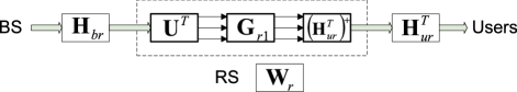
Figure 2: Structure of the optimal RS transceiver for downlink transmission

To obtain the power allocation matrix $\mathbf{G}_{r1}=\text{diag}(p_{r1},\cdots,p_{rN_{U}})$, we simply let the amplification coefficients at the RS for all streams to be identical. Denote each column of $(\mathbf{H}_{ur}^{T})^{{\dagger}}$ as $\mathbf{q}_{i}$. Since each downlink data stream is received by $\mathbf{u}_{i}^{T}$, amplified by $p_{ri}$, and forwarded by $\mathbf{q}_{i}$, we design $p_{ri}$ to ensure that each $p_{ri}\mathbf{q}_{i}\mathbf{u}_{i}^{T}$ has the same norm.

Our next task is to design the receive weighting matrix $\mathbf{U}$. Upon substituting (35), the optimization problem (31) can be rewritten as

$$\underset{\mathbf{U}}{\max~{}} \frac{1}{2}\sum_{i=1}^{N_{U}}\log_{2}\big{(}1+\frac{p_{ri}^{2}\lvert\mathbf{u}_{i}^{T}\mathbf{H}_{br}\mathbf{w}_{bti}\rvert^{2}}{N_{0}p_{ri}^{2}+N_{0}}\big{)}$$ (36a)

s.t. $$\mathbf{u}_{i}^{T}\mathbf{h}_{jr}=0,~{}i\not=j,~{}~{}\lVert\mathbf{u}_{i}\rVert=1,$$ (36b)

$$\mathbf{W}_{bt}=(\mathbf{U}^{T}\mathbf{H}_{br})^{\dagger}\mathbf{G}_{r1}^{-1}\mathbf{G}_{b},$$ (36c)

$$\lVert\mathbf{w}_{bti}\rVert^{2}=P_{B}/N_{U},$$ (36d)

$$\lVert(\mathbf{H}_{ur}^{T})^{{\dagger}}\mathbf{G}_{r1}\mathbf{U}^{T}\mathbf{H}_{br}\mathbf{W}_{bt}\rVert^{2}+N_{0}\lVert(\mathbf{H}_{ur}^{T})^{{\dagger}}\mathbf{G}_{r1}\mathbf{U}^{T}\rVert^{2}$$

$$\qquad\qquad\qquad\qquad\qquad\qquad\qquad\qquad\leq P_{R}.$$ (36e)

This problem is non-convex, thereby we turn to find its suboptimal solution. Since $\mathbf{U}^{T}$ acts as the receiver at the RS in downlink transmission, we design it to maximize the “data rate” of BS-RS transmission instead of the two-phase downlink transmission.

During the BS-RS transmission, the half-duplex RS only receives signals from the BS. Therefore, we do not consider the RS transmit power constraint (36), which can be met later by adjusting $\mathbf{G}_{r1}$. Then the BS-RS transmission rate maximization problem is formulated as

$$\underset{\mathbf{U}}{\max~{}} \sum_{i=1}^{N_{U}}\log_{2}(1+\lvert\mathbf{u}_{i}^{T}\mathbf{H}_{br}\mathbf{w}_{bti}\rvert^{2}/N_{0})$$ (37a)

s.t. (36b), (36c) and (36d). (37b)

Remark 1: If $P_{R}\to\infty$, the objective function (36a) will be the same as (37a) except for the pre-log factor $1/2$, and the RS power constraint (36) can be omitted. This means that the two optimization problems are approximately equivalent when the RS has high transmit power.

Constraint (36c) shows that $\mathbf{W}_{bt}$ is a pseudo inverse of $\mathbf{U}^{T}\mathbf{H}_{br}$ with power allocation. Define $\overline{\mathbf{U}}_{i}$ as the matrix $\mathbf{U}$ with the $i$th column $\mathbf{u}_{i}$ being removed. Then using the principle of orthogonal projection[19], we obtain that

$$\lvert\mathbf{u}_{i}^{T}\mathbf{H}_{br}\mathbf{w}_{bti}\rvert/\lVert\mathbf{w}_{bti}\rVert$$

$$= \lVert\mathbf{u}_{i}^{T}\mathbf{H}_{br}(\mathbf{I}-\mathbf{H}_{br}^{H}\overline{\mathbf{U}}_{i}^{*}(\overline{\mathbf{U}}_{i}^{T}\mathbf{H}_{br}\mathbf{H}_{br}^{H}\overline{\mathbf{U}}_{i}^{*})^{-1}\overline{\mathbf{U}}_{i}^{T}\mathbf{H}_{br})\rVert$$

$$\triangleq \lVert\mathbf{u}_{i}^{T}\mathbf{H}_{br}\mathbf{S}_{\bot}(\overline{\mathbf{U}}_{i}^{T}\mathbf{H}_{br})\rVert.$$

Substituting this expression and (36d) into (37a), then the problem (37) can be rewritten as

$$\underset{\mathbf{U}}{\max~{}} \sum_{i=1}^{N_{U}}\log_{2}(1+\frac{P_{B}}{N_{U}N_{0}}\lVert\mathbf{u}_{i}^{T}\mathbf{H}_{br}\mathbf{S}_{\perp}(\overline{\mathbf{U}}_{i}^{T}\mathbf{H}_{br})\rVert^{2})$$

s.t. $$\mathbf{u}_{i}^{T}\mathbf{h}_{jr}=0,~{}i\not=j,~{}~{}\lVert\mathbf{u}_{i}\rVert=1.$$ (38)

Constraints (36c) and (36d) are omitted since the objective function does not rely on $\mathbf{W}_{bt}$ now.

Solving problem (IV-B1) is nontrivial because we need to jointly design all $\mathbf{u}_{i}$. To obtain a low-complexity solution, we employ alternating optimization [14] again. We first initialize $\mathbf{U}=\mathbf{0}$. Then we alternately optimize each of the $N_{U}$ columns of $\mathbf{U}$. In each step, we optimize the $i$th column $\mathbf{u}_{i}$ by solving the problem (IV-B1) with all other columns $\overline{\mathbf{U}}_{i}$ being fixed. After each step, we renew the matrix $\mathbf{U}$ by replacing its $i$th column by the optimized $\mathbf{u}_{i}$. The procedure stops when the value of objective function in (IV-B1) does not increase any more. Simulations show that the procedure always converges after each of the $N_{U}$ columns has been optimized once.

In the above procedure, we need to solve the optimization problem (IV-B1) with fixed $\overline{\mathbf{U}}_{i}$. Note that the constraint $\mathbf{u}_{i}^{T}\mathbf{h}_{jr}=0$, $i\not=j$ can be rewritten as $\mathbf{u}_{i}^{T}\overline{\mathbf{H}}_{ir}=\mathbf{0}$. Any feasible $\mathbf{u}_{i}$ must lie in the orthogonal subspace of $\overline{\mathbf{H}}_{ir}$. Therefore, we have

$$\mathbf{u}_{i}=\mathbf{S}_{\bot}(\overline{\mathbf{H}}_{ir})\mathbf{x},$$ (39)

where $\mathbf{x}$ is an arbitrary vector. Then the optimization problem (IV-B1) with fixed $\overline{\mathbf{U}}_{i}$ can be rewritten as follows by substituting (39),

$$\underset{\mathbf{x}}{\max~{}} \lVert\mathbf{x}^{T}\mathbf{S}_{\bot}(\overline{\mathbf{H}}_{ir})^{T}\mathbf{H}_{br}S_{\bot}(\overline{\mathbf{U}}_{i}^{T}\mathbf{H}_{br})\rVert$$

s.t. $$\lVert\mathbf{x}\rVert=1.$$ (40)

The optimal value of $\mathbf{x}$ is the left singular vector of $\mathbf{S}_{\bot}(\overline{\mathbf{H}}_{ir})^{T}\mathbf{H}_{br}\mathbf{S}_{\bot}(\overline{\mathbf{U}}_{i}^{T}\mathbf{H}_{br})$ corresponding to its largest singular value [19]. Then from (39), we can obtain the optimal $\mathbf{u}_{i}$.

Substituting the optimization result $\mathbf{U}^{\star}$ into (35), the RS weighting matrix designed for maximizing the downlink sum rate can be obtained as $\mathbf{W}_{r}^{\star 1}=(\mathbf{H}_{ur}^{T})^{{\dagger}}\mathbf{G}_{r1}{\mathbf{U}^{\star}}^{T}$.

IV-B2 Design of $\mathbf{W}_{r}$ From Subproblem (33)

We can also show that the optimal RS weighting matrix that maximizes the uplink sum rate has the following structure,

$$\mathbf{W}_{r}^{\star 2}=\mathbf{U}^{\star}\mathbf{G}_{r2}\mathbf{H}_{ur}^{{\dagger}},$$ (41)

where $\mathbf{U}^{\star}$ and $\mathbf{G}_{r2}$ can be obtained similarly as in the last subsection. We do not present the detailed derivation for concision.

TABLE II: Comparison of Computational Complexity

	RS		BS
	major operations	complexity	major operations	complexity
ZF scheme	pseudo inverse of a $N_{R}\times 2N_{U}$ matrix	$\mathcal{O}(N_{R}N_{U}^{2})$	none	0
SA scheme	pseudo inverse of a $N_{R}\times N_{U}$ matrix	$\mathcal{O}(N_{R}N_{U}^{2})$	pseudo inverse of a $N_{B}\times N_{U}$ matrix	$\mathcal{O}(N_{B}N_{U}^{2})$
Balanced scheme	pseudo inverse of a $N_{R}\times N_{U}$ matrix, $N_{U}$ times of SVD of $N_{R}\times(N_{B}-N_{U}+1)$ matrix	$\mathcal{O}(N_{R}N_{U}^{2})+$ $\mathcal{O}(N_{R}N_{U}(N_{B}-N_{U}+1)^{2})$	pseudo inverse of $N_{B}\times N_{U}$ matrices	$\mathcal{O}(N_{B}N_{U}^{2})$

IV-B3 Balancing $R_{U}$ and $R_{D}$ to Maximize Bidirectional Sum Rate

Consider that bidirectional sum rate $R_{S}=R_{U}+R_{D}$, while $\mathbf{W}_{r}^{\star 1}$ and $\mathbf{W}_{r}^{\star 2}$ are respectively optimized for $R_{U}$ and $R_{D}$. To improve $R_{S}$, we propose the following RS weighting matrix,

$$\mathbf{W}_{r}^{BL}=c_{\gamma}(\gamma\mathbf{W}_{r}^{\star 1}+(1-\gamma)\mathbf{W}_{r}^{\star 2}),$$ (42)

where the power adjusting factor $\gamma$, $0\leq\gamma\leq 1$, is used for controlling the power proportion to $\mathbf{W}_{r}^{\star 1}$ and $\mathbf{W}_{r}^{\star 2}$ to balance the uplink and downlink sum rate, $c_{\gamma}$ is used to meet the total RS transmit power constraint. In practical systems, after obtaining $\mathbf{W}_{r}^{\star 1}$ and $\mathbf{W}_{r}^{\star 2}$, the RS can search for an optimal $\gamma$ that maximizes the bidirectional sum rate.

Remark 2: In a TWR system with single user and single-antenna BS, $\mathbf{W}_{r}^{BL}$ turns out to be a maximal-ratio combination and maximal-ratio transmission (MRC-MRT) weighting matrix. It is shown in [2] that the bidirectional sum rate gap between MRC-MRT and the optimal scheme is no more than 0.2bps/Hz. Though in multi-user multi-antenna TWR system, we cannot draw the same conclusion via rigorously analysis, the simulation results in section V will show that such a balanced solution performs closely to the alternating optimization solution.

Remark 3: By substituting $\mathbf{W}_{r}^{\star 1}$ and $\mathbf{W}_{r}^{\star 2}$ into (42), we have

$$\mathbf{W}_{r}^{BL}=c_{\gamma}(\gamma(\mathbf{H}_{ur}^{T})^{{\dagger}}\mathbf{G}_{r1}\mathbf{U}^{\star T}+(1-\gamma)\mathbf{U}^{\star}\mathbf{G}_{r2}\mathbf{H}_{ur}^{{\dagger}}).$$ (43)

As shown in (39), each column of matrix $\mathbf{U}^{\star}$ lies in the orthogonal subspace of $\overline{\mathbf{H}}_{ir}$, i.e., $\mathbf{u}_{i}^{\star}\in\mathbf{S}_{\bot}(\overline{\mathbf{H}}_{ir})$. The $i$th column of $(\mathbf{H}_{ur}^{T})^{\dagger}$ also lies in that orthogonal subspace, i.e., $\mathbf{q}_{i}\in\mathbf{S}_{\bot}(\overline{\mathbf{H}}_{ir})$.

When $N_{R}=N_{U}$, i.e., the number of RS antennas equals to the number of users, the matrix $\overline{\mathbf{H}}_{ir}$ is a $N_{R}\times(N_{R}-1)$ matrix. Therefore, the rank of its orthogonal subspace $\mathbf{S}_{\bot}(\overline{\mathbf{H}}_{ir})$ is one. Since both of $\mathbf{u}_{i}^{\star}$ and $\mathbf{q}_{i}$ lie in the same rank-1 subspace, they are linearly dependent, i.e., $\mathbf{u}_{i}^{\star}=d_{i}\mathbf{q}_{i}$, where $d_{i}$ is a scalar. Therefore, we have $\mathbf{U}^{\star}=(\mathbf{H}_{ur}^{T})^{\dagger}\mathbf{D}$, where $\mathbf{D}=\text{diag}(d_{1},\cdots,d_{N_{U}})$. Substituting this expression into (43), we obtain

$$\mathbf{W}_{r}^{BL} =(\mathbf{H}_{ur}^{T})^{\dagger}(c_{\gamma}\gamma\mathbf{G}_{r1}\mathbf{D}^{T}+c_{\gamma}(1-\gamma)\mathbf{D}\mathbf{G}_{r2})\mathbf{H}_{ur}^{\dagger}$$

$$\triangleq(\mathbf{H}_{ur}^{T})^{\dagger}\mathbf{G}_{r}^{BL}\mathbf{H}_{ur}^{\dagger},$$ (44)

where $\mathbf{G}_{r}^{BL}\triangleq c_{\gamma}\gamma\mathbf{G}_{r1}\mathbf{D}^{T}+c_{\gamma}(1-\gamma)\mathbf{D}\mathbf{G}_{r2}$ is a diagonal matrix.

Comparing (IV-B3) with the RS transceiver in the SA scheme proposed in [11, 9, 10], we see that $\mathbf{W}_{r}^{BL}$ has the same form as that of the SA scheme. Substituting (IV-B3) into (27) and (29), it is easy to show that the BS transceivers in our balanced solution also have the same forms as those in the SA scheme. This indicates that the SA scheme is a special case of the balanced solution when $N_{R}=N_{U}$. In fact, in such a setting, it is not hard to show that the solution of interference free constraints (7), (9) and (10) is unique, which is exactly the SA scheme.

IV-C Complexity Comparison

Here we compare the computational complexities of the balanced scheme and the existing ZF [8] and SA schemes [9, 10, 11].

In the ZF scheme, the major operation at the RS is to compute the pseudo inverse of a $N_{R}\times 2N_{U}$ matrix. Since all the interference are eliminated by the RS, the BS needs to do nothing. In the SA scheme, the major operations at the RS and the BS are to compute the pseudo inverses of a $N_{R}\times N_{U}$ matrix and a $N_{B}\times N_{U}$ matrix, respectively.

In the balanced scheme, to obtain the RS transceiver (42), we need to compute $\mathbf{H}_{ur}^{\dagger}$, $\mathbf{U}$, $\mathbf{G}_{r1}$ and $\mathbf{G}_{r2}$, and search for the optimal balancing factor $\gamma$. Specifically, we need to perform $N_{U}$ times of singular vector decomposition (SVD) to alternately design the $N_{U}$ columns of $\mathbf{U}$. According to (IV-B1), each SVD is performed for a $N_{R}\times(N_{B}-N_{U}+1)$ matrix. Only vector norm operation is required to compute the power allocation matrices $\mathbf{G}_{r1}$ and $\mathbf{G}_{r2}$, for which the complexity can be neglected compared with those of the pseudo inverse and SVD. The complexity of finding the optimal $\gamma$ can also be ignored, which only requires a scalar searching operation. To obtain the BS transceivers in our balanced scheme (27) and (29), we need to compute the pseudo inverses of two $N_{B}\times N_{U}$ matrices.

A widely used method for computing pseudo inverse is using SVD, which results in a complexity of $\mathcal{O}(mn^{2})$ flops to compute the pseudo inverse of a $m\times n$ matrix [21], where $m\geq n$. The complexities of the transceiver schemes are present in Table II, which shows that the complexity of the balanced scheme is on the same order as those of the SA and ZF schemes.

V Simulation Results

In this section, we evaluate the performance of the proposed transceivers and compare them with existing schemes by simulations. We assume that all channels are independent and identically distributed Rayleigh fading channels, and all simulation results are obtained by averaging over 1000 Monte-Carlo trails. For a fair comparison, we use equal power allocation at the BS and RS in all the transceiver schemes. We assume that the noise variance $N_{0}$ is identical at the BS, RS and each user. The transmit power of each user $P_{U}=1$. The BS and RS transmit power are $P_{B}$ and $P_{R}$, respectively. We define $1/N_{0}$ as the transmit SNR. Without otherwise specified, we set $N_{B}=2$, $N_{R}=4$, $N_{U}=2$, $P_{B}=P_{R}=2$, and $SNR=30$ dB.

V-A Impact of the Adjusting factor

The sum rates of balanced scheme versus the power adjusting factor $\gamma$ are shown in Fig. 3, where the upper sub-figure shows the uplink and downlink sum rates and the lower sub-figure shows the bidirectional sum rate. When $\gamma=0$, the RS weighting matrix $\mathbf{W}_{r}=\mathbf{W}_{r}^{\star 2}$, which aims to maximize the uplink sum rate. Therefore, the system achieves high uplink sum rate but low downlink sum rate in this case. By contrast, when $\gamma=1$, the system achieves high downlink rate but low uplink rate. By adjusting the value of $\gamma$, the uplink and downlink performance are balanced and higher bidirectional sum rate is achieved. The optimal $\gamma$ under this case is 0.5.

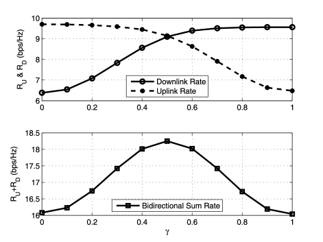
Figure 3: Sum rates vs. the power adjusting factor $\gamma$, $N_{B}$ = 2, $N_{R}$ = 4, and $N_{U}$ =2

V-B Convergence of the Alternating Optimization Solution

To study the convergence of the alternating optimization algorithm, we respectively use the proposed balanced transceiver, the ZF and SA transceivers and multiple random weighting matrices as its initial value. When using random matrices as the initial values, we pick one from multiple results that converges to the highest sum rate.

Figure 4 shows the bidirectional sum rate versus the iteration number. The sum rate converges rapidly but the converged result depends on the initial values due to the non-convexity nature of the optimization problem. Nonetheless, by using multiple random initial values, higher bidirectional sum rate can be achieved. We observe from extensive simulations that when the number of random initial values exceeds 20, the performance gain is marginal. Therefore, we can take the result with 20 random initial values as a near-optimal result. It is shown that the performance of the balanced transceiver is very close to that of the near-optimal result. In the following, we will use the balanced transceiver as the initial value for the alternating optimization.

Figure 4: Convergence of the alternating optimization algorithm with different initial values, $N_{B}$ = 2, $N_{R}$ = 4, and $N_{U}$ =2

V-C Comparison among Different Transceivers

We compare the bidirectional sum rates of alternating optimization solution and the balanced transceiver with those of the ZF [8] and SA schemes [11, 9, 10]. We also compare with a minimum-mean-square-error (MMSE) transceiver without the interference free constraints, where the MMSE BS transceiver and MMSE RS transceiver were alternately optimized [22].

Figure 5 shows the impact of the antenna number of the RS, where “Al-Opt” denotes the alternating optimization solution. When there are two users, the ZF scheme needs at least 4 antennas at the RS to cancel all the interference, while the SA scheme only needs 2 antennas. From the simulation results, we see that when $N_{R}\leq 4$ the sum rate of the ZF scheme reduces sharply due to the residual IUI, but the SA scheme performs much better. When $N_{R}>4$, the ZF scheme becomes superior because it can remove all IUI but the SA scheme suffers from a power loss when aligning the downlink signals with the uplink signals. The sum rate of the balanced transceiver is close to that of the alternating optimization solution, both are higher than the existing ZF and SA schemes for any antenna number at the RS.

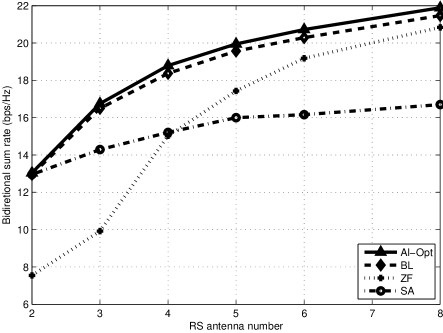
Figure 5: Sum rates of four transceivers vs. RS antenna number, $N_{B}$ = 2, and $N_{U}$ =2

Figure 6 shows the impact of the user number on the performance of different transceivers. We set $N_{B}=N_{R}=4$, and $P_{B}=P_{R}=4$. Round robin scheduler is applied, where the scheduled user number $N_{U}$ is from 1 to 4. It shows that the performance of the ZF scheme degrades severely when $N_{U}>2$ because the four-antenna RS can not cancel all IUI. With the SA scheme, the proposed balanced scheme and the alternating optimization solution, the system achieves the highest bidirectional sum rate when three users are scheduled, where both the balanced scheme and alternating optimization result have about 2bps/Hz sum rate gain over the SA scheme. When $N_{U}=4$, we see that the performance of the balanced transceiver and the SA scheme are exactly the same. This agrees well with our earlier analysis in Remark 3.

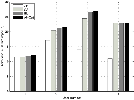
Figure 6: Sum rate of four transceivers vs. user number, $N_{B}$ = 4, and $N_{R}$ = 4

In Fig. 7 we compare the sum rate of the interference free transceiver schemes with the MMSE transceiver [22]. We can see that our balanced scheme provides higher sum rate than the existing ZF and SA schemes in a wide range of transmit SNR. The MMSE scheme is slightly superior to our balanced scheme in low SNR region, but is inferior to the proposed scheme in high SNR region. This is because the MMSE solution in [22] is obtained via alternating optimization, which is not guaranteed to be globally optimal. In high SNR region, the system is interference-limited, therefore the proposed scheme outperforms the MMSE solution by removing all the interference.

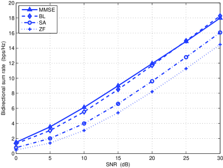
Figure 7: Sum rate vs. SNR, $N_{B}$ = 2, $N_{R}$ = 4, and $N_{U}$ = 2.

In Fig. 8, we provide the sum rate under each single channel realization to understand the behavior of the IUI free transceivers. We see that the ZF and SA schemes perform differently for a given channel. The ZF scheme requires the RS to separate all the signals transmitted by the users and BS, and performs well only when the channel vectors from the users and the BS are mutually orthogonal. Contrarily, the SA scheme needs to align the signals transmitted by the BS onto the same directions of the signals transmitted by the users, and thus performs well only when the channel vectors from the users and those from the BS have the same direction. Our balanced scheme can adaptively adjust transmission strategy depending on the channel condition to ensure IUI free without the requirements for channel “orthogonalization” or “alignment”. Therefore, its sum rate is always higher than those of ZF and SA schemes.

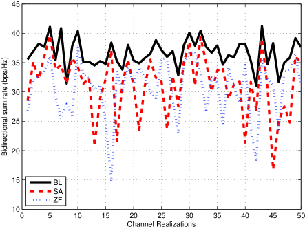
Figure 8: Sum rate under different channel realizations, $N_{B}$ = 2, $N_{R}$ = 4, and $N_{U}$ = 2.

In Fig. 9, we compare the outage probabilities of the IUI free transceivers with $10^{5}$ Monte-Carlo trails, where the system is in outage if its bidirectional sum rate drops below a given threshold, which is set as 2bps/Hz. We see that our balanced scheme achieves much lower outage probability than both the ZF and SA schemes. Moreover, since the sum rate of the balanced scheme is always “riding on the peak” of the ZF and SA schemes as shown in Fig. 8, the balanced scheme achieves higher diversity gain, and its outage probability decreases much faster than those of the ZF and SA schemes as the SNR increases.

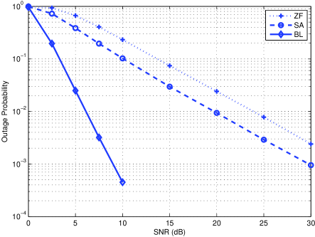
Figure 9: Outage probability vs. SNR, $N_{B}$ = 2, $N_{R}$ = 4, and $N_{U}$ = 2.

VI Conclusion

In this paper, we have designed transceiver for multi-user multi-antenna two-way relay systems. We first employed alternating optimization to find the BS and RS transceivers that maximizes the bidirectional sum rate under interference free constraints. We proceeded to propose a low complexity balanced transceiver scheme. By analyzing the solution of the alternating optimization in high transmit power region, we find that zero-forcing BS transceivers are asymptotically optimal. Given the BS transceivers, we designed the RS transceivers by respectively maximizing the uplink and downlink rate, which are then combined with a power adjustment factor to maximize the bidirectional sum rate. Existing signal alignment scheme was shown as a special case of the balance scheme where the relay antenna number equals to the user number. Simulation results showed that the performance gap between the balanced scheme and the alternating optimization solution is minor. In general system settings, the bidirectional sum rate of the balanced transceiver is higher than the existing signal alignment and zero-forcing schemes.

Proof of the Optimal Structure of $\mathbf{W}_{r}$ in (35)

Define $\mathbf{V}_{ur}\in\mathbb{C}^{N_{R}\times N_{U}}$ as a matrix consisting of the $N_{U}$ singular vectors of $\mathbf{H}_{ur}^{T}$, and $\mathbf{V}_{ur}^{\perp}\in\mathbb{C}^{N_{R}\times(N_{R}-N_{U})}$ as a matrix consisting of the $N_{R}-N_{U}$ singular vectors of the orthogonal subspace of $\mathbf{H}_{ur}^{T}$. Then $\mathbf{V}_{F}=[\mathbf{V}_{ur}~{}\mathbf{V}_{ur}^{\perp}]$ is a unitary matrix, and $\mathbf{W}_{r}$ can be expressed as

$$\mathbf{W}_{r}=\mathbf{V}_{F}\mathbf{V}_{F}^{H}\mathbf{W}_{r}=\mathbf{V}_{ur}\mathbf{A}^{T}+\mathbf{V}_{ur}^{\perp}\mathbf{B}^{T},$$ (45)

where $\mathbf{A}\in\mathbb{C}^{N_{R}\times N_{U}}$, $\mathbf{B}\in\mathbb{C}^{N_{R}\times(N_{R}-N_{U})}$ are two arbitrary matrices.

Since $\mathbf{h}_{ir}^{T}\mathbf{V}_{ur}^{\perp}=\mathbf{0}$, from (III), the downlink sum rate $R_{D}$ can be written as

$$R_{D} =\frac{1}{2}\sum_{i=1}^{N_{U}}\log_{2}(1+\frac{\lvert\mathbf{h}_{ir}^{T}\mathbf{V}_{ur}\mathbf{A}^{T}\mathbf{H}_{br}\mathbf{w}_{bti}\rvert^{2}}{N_{0}\lVert\mathbf{h}_{ir}^{T}\mathbf{V}_{ur}\mathbf{A}^{T}\rVert^{2}+N_{0}}).$$ (46)

Substituting (45) into (27), we have $\mathbf{W}_{bt}=(\mathbf{H}_{ur}^{T}\mathbf{V}_{ur}\mathbf{A}^{T}\mathbf{H}_{br})^{{\dagger}}\mathbf{G}_{b}$, which is not a function of $\mathbf{B}$. Therefore, the value of $\mathbf{B}$ does not affect the constraints (27) and (28) in problem (31). According to (46), the objective function $R_{D}$ of problem (31) also does not depend on $\mathbf{B}$.

Substituting (45) into (10), we obtain $\mathbf{h}_{ir}^{T}\mathbf{W}_{r}\mathbf{h}_{jr}=\mathbf{h}_{ir}^{T}\mathbf{V}_{ur}\mathbf{A}^{T}\mathbf{h}_{jr}=0,i\not=j$, which shows that the value of $\mathbf{B}$ does not affect the constraint (10) either.

We can show that the RS transmit power is minimized when $\mathbf{B}=\mathbf{0}$ as follows,

$$\lVert\mathbf{W}_{r}\mathbf{H}_{br}\mathbf{W}_{bt}\rVert^{2}+N_{0}\lVert\mathbf{W}_{r}\rVert^{2}$$

$$= \lVert\mathbf{V}_{ur}\mathbf{A}^{T}\mathbf{H}_{br}\mathbf{W}_{bt}\rVert^{2}+\lVert\mathbf{V}_{ur}^{\perp}\mathbf{B}^{T}\mathbf{H}_{br}\mathbf{W}_{bt}\rVert^{2}$$

$$+N_{0}\lVert\mathbf{V}_{ur}\mathbf{A}^{T}\rVert^{2}+N_{0}\lVert\mathbf{V}_{ur}^{\perp}\mathbf{B}^{T}\rVert^{2}$$

$$\geq P_{B}\lVert\mathbf{V}_{ur}\mathbf{A}^{T}\mathbf{H}_{br}\mathbf{W}_{bt}\rVert^{2}+N_{0}\lVert\mathbf{V}_{ur}\mathbf{A}^{T}\rVert^{2}.$$

It indicates that for any given $\mathbf{W}_{r}=\mathbf{V}_{ur}\mathbf{A}^{T}+\mathbf{V}_{ur}^{\perp}\mathbf{B}^{T}$, we can always find a $\mathbf{W}_{r}^{\star}=\mathbf{V}_{ur}\mathbf{A}^{T}$, which achieves the same downlink rate $R_{D}$ as that with $\mathbf{W}_{r}$ but consumes less RS power. Therefore, the optimal $\mathbf{W}_{r}$ for (31) should has the structure of $\mathbf{W}_{r}=\mathbf{V}_{ur}\mathbf{A}^{T}$.

Denote the singular value decomposition of $\mathbf{H}_{ur}^{T}$ as $\mathbf{U}_{ur}\mathbf{D}_{ur}\mathbf{V}_{ur}^{H}$, where $\mathbf{D}_{ur},\mathbf{U}_{ur}$ are both non-singular matrix, then we have

$$\mathbf{W}_{r} =\mathbf{V}_{ur}\mathbf{A}^{T}=\mathbf{V}_{ur}(\mathbf{D}_{ur}^{-1}\mathbf{U}_{ur}^{H}\mathbf{U}_{ur}\mathbf{D}_{ur})\mathbf{A}^{T}$$

$$=(\mathbf{H}_{ur}^{T})^{{\dagger}}\mathbf{U}_{ur}\mathbf{D}_{ur}\mathbf{A}^{T}\triangleq(\mathbf{H}_{ur}^{T})^{{\dagger}}\mathbf{M}^{T},$$

where $\mathbf{M}^{T}\triangleq\mathbf{U}_{ur}\mathbf{D}_{ur}\mathbf{A}^{T}$. Divide the matrix $\mathbf{M}=(\mathbf{m}_{1},\cdots,\mathbf{m}_{N_{U}})$ into two matrices, $\mathbf{U}=(\mathbf{u}_{1},\cdots,\mathbf{u}_{N_{U}})$ and $\mathbf{G}_{r1}=\text{diag}(p_{r1},\cdots,p_{rN_{U}})$, where $\mathbf{u}_{j}\triangleq\mathbf{m}_{j}/\lVert\mathbf{m}_{j}\rVert$ and $p_{rj}\triangleq\lVert\mathbf{m}_{j}\rVert$. Finally, we have $\mathbf{W}_{r}=(\mathbf{H}_{ur}^{T})^{{\dagger}}\mathbf{G}_{r1}\mathbf{U}^{T}$.

Can Sun received his B.S. degree in 2006 from Beijing University of Aeronautics and Astronautics (BUAA, now renamed as Beihang University). He is currently a Ph.D student in signal and information processing in the School of Electronics and Information Engineering, BUAA, Beijing, China. Since Apr. 2009 to Mar. 2010, he was a visiting student with the University of Sydney, NSW, Australia. His research interests include coordinated multi-point transmission, relay communication and energy efficient transmission.

Chenyang Yang received her MSE and PhD degrees in 1989 and 1997 in Electrical Engineering, from Beijing University of Aeronautics and Astronautics (BUAA, now renamed as Beihang University). She is now a full professor in the School of Electronics and Information Engineering, BUAA. She has published various papers and filed many patents in the fields of signal processing and wireless communications. She was nominated as an Outstanding Young Professor of Beijing in 1995 and was supported by the 1st Teaching and Research Award Program for Outstanding Young Teachers of Higher Education Institutions by Ministry of Education (P.R.C. ”TRAPOYT”) during 1999-2004. Currently, she serves as an associate editor for IEEE Transactions on Wireless Communications, an associate editor-in-chief of Chinese Journal of Communications and an associate editor-in-chief of Chinese Journal of Signal Processing. She is the chair of Beijing chapter of IEEE Communications Society. She has ever served as TPC members for many IEEE conferences such as ICC and GLOBECOM. Her recent research interests include network MIMO, energy efficient transmission and interference management in multi-cell systems.

Yonghui Li (M’04-SM’09) received his PhD degree in November 2002 from Beijing University of Aeronautics and Astronautics. From 1999 - 2003, he was affiliated with Linkair Communication Inc, where he held a position of project manager with responsibility for the design of physical layer solutions for the LAS-CDMA system. Since 2003, he has been with the Centre of Excellence in Telecommunications, the University of Sydney, Australia. He is now an Associate Professor in School of Electrical and Information Engineering, University of Sydney. He is also currently the Australian Queen Elizabeth II fellow. His current research interests are in the area of wireless communications, with a particular focus on MIMO, cooperative communications, coding techniques and wireless sensor networks. He holds a number of patents granted and pending in these fields. He is an executive editor for European Transactions on Telecommunications (ETT), Editor for Journal of Networks, and was an Associate Editor for EURASIP Journal on Wireless Communications and Networking from 2006-2008. He also served as the Leading Editor for special issue on ”advances in error control coding techniques” in EURASIP Journal on Wireless Communications and Networking, He has also been involved in the technical committee of several international conferences, such as ICC, Globecom, etc.

Branka Vucetic (M’83-SM’00-F’03) received the B.S.E.E., M.S.E.E., and Ph.D. degrees in 1972, 1978, and 1982, respectively, in electrical engineering, from The University of Belgrade, Belgrade, Yugoslavia. During her career she has held various research and academic positions in Yugoslavia, Australia, and the UK. Since 1986, she has been with the Sydney University School of Electrical and Information Engineering in Sydney, Australia. She is currently the Director of Centre of Excellence in Telecommunications at Sydney University. Her research interests include wireless communications, digital communication theory, coding, and multi-user detection. In the past decade she has been working on a number of industry sponsored projects in wireless communications and mobile Internet. She has taught a wide range of undergraduate, postgraduate, and continuing education courses worldwide. Prof. Vucetic co-authored four books and more than two hundred papers in telecommunications journals and conference proceedings.

References

- [1] R. Louie, Y. Li, and B. Vucetic, “Practical physical layer network coding for two-way relay channels: performance analysis and comparison,” IEEE Trans. Wireless Commun., vol. 9, no. 2, pp. 764 –777, Feb. 2010.
- [2] R. Zhang, Y.-C. Liang, C. C. Chai, and S. Cui, “Optimal beamforming for two-way multi-antenna relay channel with analogue network coding,” IEEE J. Select. Areas Commun., vol. 27, no. 5, pp. 699 –712, June 2009.
- [3] T. J. Oechtering, E. A. Jorswieck, R. F. Wyrembelski, and H. Boche, “On the optimal transmit strategy for the MIMO bidirectional broadcast channel,” IEEE Trans. Commun., vol. 57, no. 12, pp. 3817–3826, Dec. 2009.
- [4] M. Chen and A. Yener, “Multiuser two-way relaying: detection and interference management strategies,” IEEE Trans. Wireless Commun., vol. 8, no. 8, pp. 4296 –4305, Aug. 2009.
- [5] J. Joung and A. H. Sayed, “Multiuser two-way amplify-and-forward relay processing and power control methods for beamforming systems,” IEEE Trans. Signal Processing, vol. 58, no. 3, pp. 1833 –1846, Mar. 2010.
- [6] M. Chen and A. Yener, “Power allocation for F/TDMA multiuser two-way relay networks,” IEEE Trans. Wireless Commun., vol. 9, no. 2, pp. 546–551, Feb. 2010.
- [7] K. Jitvanichphaibool, R. Zhang, and Y.-C. Liang, “Optimal resource allocation for two-way relay-assisted OFDMA,” IEEE Trans. Veh. Technol., vol. 58, no. 7, pp. 3311–3321, Sept. 2009.
- [8] C. Esli and A. Wittneben, “Multiuser MIMO two-way relaying for cellular communications,” in Proc. IEEE PIMRC, Sept. 2008, pp. 1 –6.
- [9] S. Toh and D. T. M. Slock, “A linear beamforming scheme for multi-user MIMO AF two-phase two-way relaying,” in Proc. IEEE PIMRC, Sept. 2009, pp. 1003–1007.
- [10] Z. Ding, I. Krikidis, J. Thompson, and K. K. Leung, “Physical layer network coding and precoding for the two-way relay channel in cellular systems,” IEEE Trans. Signal Processing, vol. 59, no. 2, pp. 696–712, Jan. 2011.
- [11] H. J. Yang, B. C. Jung, and J. Chun, “Zero-forcing-based two-phase relaying with multiple mobile stations,” in Proc. 42nd Asilomar Conf. Signals, Systems and Computers, 2008, pp. 351–355.
- [12] N. Lee, J.-B. Lim, and J. Chun, “Degrees of freedom of the MIMO Y channel: Signal space alignment for network coding,” IEEE Trans. Inform. Theory, vol. 56, no. 7, pp. 3332–3342, July 2010.
- [13] B. Rankov and A. Wittneben, “Spectral efficient protocols for half-duplex fading relay channels,” IEEE J. Select. Areas Commun., vol. 25, no. 2, pp. 379 –389, Feb. 2007.
- [14] J. C. Bezdek and R. J. Hathaway, “Some notes on alternating optimization,” in Proc. AFSS International Conference on Fuzzy Systems, Feb. 2002, pp. 288–300.
- [15] M. Mohseni, R. Zhang, and J. M. Cioffi, “Optimized transmission for fading multiple-access and broadcast channels with multiple antennas,” IEEE J. Select. Areas Commun., vol. 24, no. 8, pp. 1627–1639, Aug. 2006.
- [16] R. L. Burden and J. D. Faires, Numerical Analysis. Pacific Grove, CA: Brooks/Cole, 2000.
- [17] Z. Luo and W. Yu, “An introduction to convex optimization for communications and signal processing,” IEEE J. Select. Areas Commun., vol. 24, no. 8, pp. 1426–1438, Aug. 2006.
- [18] M. Grant, S. Boyd, and Y. Ye. (2009) CVX: MATLAB software for disciplined convex programming. [online] available: http://www.stanford.edu/ boyd/cvx.
- [19] H. V. Trees, Detection, Estimation, and Modulation Theory. Part IV: Optimum Array Processing. New York: Wiley, 2002.
- [20] A. Wiesel, Y. C. Eldar, and S. Shamai, “Zero-forcing precoding and generalized inverses,” IEEE Trans. Signal Processing, vol. 56, no. 9, pp. 4409–4418, Sept. 2008.
- [21] G. Xu, H. Zha, G. Golub, and T. Kailath, “Fast algorithms for updating signal subspaces,” IEEE Trans. Circuits Syst. II, vol. 41, no. 8, pp. 537–549, Aug. 1994.
- [22] H. Degenhardt, T. Unger, and A. Klein, “Self-interference aware MMSE filter design for a cellular multi-antenna two-way relaying scenario,” in Proc. ISWCS, 2011, pp. 261–265.