Global and local expansion of magnetic clouds in the inner heliosphere

Abstract

Context. Observations of magnetic clouds (MCs) are consistent with the presence of flux ropes detected in the solar wind (SW) a few days after their expulsion from the Sun as coronal mass ejections (CMEs).

Aims. Both the in situ observations of plasma velocity profiles and the increase of their size with solar distance show that MCs are typically expanding structures. The aim of this work is to derive the expansion properties of MCs in the inner heliosphere from 0.3 to 1 AU.

Methods. We analyze MCs observed by the two Helios spacecraft using in situ magnetic field and velocity measurements. We split the sample in two subsets: those MCs with a velocity profile that is significantly perturbed from the expected linear profile and those that are not.

From the slope of the in situ measured bulk velocity along the Sun-Earth direction, we compute an expansion speed with respect to the cloud center for each of the analyzed MCs.

Results. We analyze how the expansion speed depends on the MC size, the translation velocity, and the heliocentric distance, finding that all MCs in the subset of non-perturbed MCs expand with almost the same non-dimensional expansion rate ($\zeta$). We find departures from this general rule for $\zeta$ only for perturbed MCs, and we interpret the departures as the consequence of a local and strong SW perturbation by SW fast streams, affecting the MC even inside its interior, in addition to the direct interaction region between the SW and the MC. We also compute the dependence of the mean total SW pressure on the solar distance and we confirm that the decrease of the total SW pressure with distance is the main origin of the observed MC expansion rate. We found that $\zeta$ was $0.91\pm 0.23$ for non-perturbed MCs while $\zeta$ was $0.48\pm 0.79$ for perturbed MCs, the larger spread in the last ones being due to the influence of the solar wind local environment conditions on the expansion.

1 Introduction

Magnetic clouds (MCs) are magnetized plasma structures forming a particular subset of interplanetary coronal mass ejections (ICMEs, e.g., Burlaga, 1995). MCs are transient structures in the solar wind (SW) defined by an enhanced magnetic field with respect to that found in the surrounding SW with a coherent rotation of the field of the order of about a day when these structures are observed at 1 AU (Burlaga et al., 1981). A lower proton temperature than the expected one in the SW with the same velocity is another signature of MCs that complement their identification (e.g., Richardson & Cane, 1995; Marsch et al., 2009).

Figure 1: Examples of two analyzed MCs that are not significantly perturbed by a fast flow. The MC center was observed at 07-Jan-1975 10:39 and 04-Mar-1975 21:37 UT, for panels (a,c) and (b,d), respectively. The vertical dashed lines define the MC boundaries. (a,b) $V_{x}$ is the observed velocity component in the radial direction from the Sun, expressed in km per second. The straight line is the linear least square fit of the velocity in the time interval where an almost linear trend is present (where the observations are presented as a solid line). The linear fitting is extrapolated to the borders of the MC, which are marked with circles. (c,d) $B_{y}$ is the magnetic field component, in nT, both orthogonal to the MC axis and to the spacecraft trajectory, while the solid line represents $F_{y}$, which is the accumulated flux of $B_{y}$ (Eq. 7). The extremum of $F_{y}$ (proxy of the cloud center) is indicated with diamonds (A color version is available in the electronic version).

MCs interact with their environment during their journey in the solar wind (SW) from the Sun to the outer heliosphere and, since the SW pressure (magnetic plus plasma) decreases for increasing heliocentric distance, an expansion of MCs is expected. In a heliospheric frame, the in situ observed bulk plasma velocity typically decreases in magnitude from the front to the back inside MCs, confirming the expectation that MCs are expanding objects in the SW. Furthermore, from observations of large samples of MCs observed at different heliocentric distance, it has been shown that the size of MCs increases for larger heliocentric distances (Leitner et al., 2007, and references therein).

These structures have an initial expansion from their origin in the Sun, as shown from observations of radial expansion at the corona; e.g., an example of the leading edge of a CME traveling faster than its core is shown in Figure 6 of Tripathi et al. (2006). However their subsequent expansion mainly will be given by the environmental (SW) conditions as a consequence of force balance (Démoulin & Dasso, 2009).

Dynamical models have been used to describe clouds in expansion, either considering only a radial expansion (e.g., Farrugia et al., 1993; Osherovich et al., 1993; Farrugia et al., 1997; Nakwacki et al., 2008b), or expansion in both the radial and axial directions (e.g., Shimazu & Vandas, 2002; Berdichevsky et al., 2003; Dasso et al., 2007; Nakwacki et al., 2008a; Démoulin & Dasso, 2009). The main aim of these models is to take into account the evolution of the magnetic field as the MC crosses the spacecraft. Another goal is to correct the effect of mixing spatial-variation/time-evolution in the one-point observations to obtain a better determination of the MC field configuration. The expansion of several magnetic clouds has been analyzed previously by fitting different velocity models to the data (Farrugia et al., 1993; Shimazu & Vandas, 2002; Berdichevsky et al., 2003; Vandas et al., 2005; Yurchyshyn et al., 2006; Dasso et al., 2007; Mandrini et al., 2007; Démoulin et al., 2008).

The expansion of some MCs is not always well marked with in situ velocity measurements. This is in particular the case for small MCs or those overtaken by fast streams. Slow magnetic clouds, with velocities lower than or of the order of $400$ km/s, in general have small sizes, low magnetic field strengths, and only a few of them present shocks or sheaths (e.g., Tsurutani et al., 2004). Fast streams overtaking magnetic clouds from behind can compress the magnetic field in the rear for the overtaken MC, for instance in some cases forming large structures called merged interaction regions (e.g., Burlaga et al., 2003). The interaction between a stream and an MC can affect the internal structure of the cloud (e.g., as shown from numerical simulations by Xiong et al., 2007). The difference between the velocities of the front and back boundaries, called $\Delta V_{\rm obs}$, was frequently used to qualify how important the expansion of an observed MC is. A larger $\Delta V_{\rm obs}$ is favorable for the presence of shocks surrounding the MC, especially for the presence of a backward shock (Gosling et al., 1994). A large $\Delta V_{\rm obs}$ is less important for the presence of a frontal shock since a frontal shock is also created by a large difference between the MC global velocity and the overtaken SW velocity.

The quantity $\Delta V_{\rm obs}$ is a good proxy of the time variation of the global size of the MC, however, $\Delta V_{\rm obs}$ does not express how fast the expansion of an element of fluid is, since $\Delta V_{\rm obs}$ depends strongly on how big the studied MC is. For example the MC observed by ACE at 1 AU on 29 October 2004 (Mandrini et al., 2007) is formed by a flux rope with a large radius, $R\approx 0.17$ AU, and it also has a large $\Delta V_{\rm obs}\approx 400$ km s^-1, and so, at first sight, it can be qualified as a very rapidly expanding MC. However, let suppose that the same MC would have most its flux having been reconnected with the encountered SW during the transit from the Sun, as has been observed in some cases (e.g., Dasso et al., 2006, 2007), so that only the flux rope core would have been observed as a MC. If the remaining flux rope would have a radius of only $10^{-2}$ AU, it would have shown $\Delta V_{\rm obs}\approx 400/17\approx 24$ km s^-1, so it would have been qualified as a slowly expanding MC.

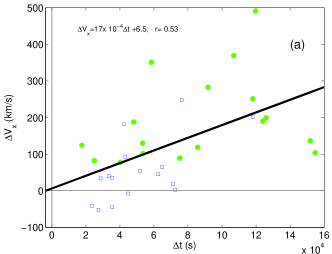
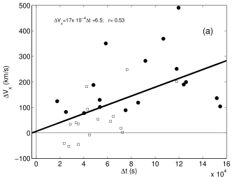
More generally, small flux ropes are expected to have intrinsically small $\Delta V_{\rm obs}$, an expectation confirmed by the data (Fig. 3a,b). MCs have a broad range of sizes, with flux rope radii of a few $0.1$ AU down to a few $10^{-3}$ AU (Lynch et al., 2003; Feng et al., 2007), and it is necessary to quantify their expansion rate independently of their size. In this study, we analyze the expansion of MCs in the inner heliosphere, and find a non-dimensional expansion coefficient ($\zeta$), which can be quantified from one-point in situ observations of the bulk velocity time profile of the cloud. We demonstrate that $\zeta$ characterizes the expansion rate of the MC, independently of its size.

We first describe the data used, and then the method to define the main properties of the MC (Sect. 2). In Sect. 3, we analyze the properties of the MC expansion, defining a proper expansion coefficient. We derive specific properties of two groups of MCs, defined from their interaction with the SW environment. Then, we relate the MC expansion rate to the decrease of the total SW pressure with solar distance. We summarize our results in Sect. 4 and conclude in Sect. 5.

Figure 2: Examples of two analyzed MCs that are perturbed by a fast flow as seen in the upper panels. The MC center was observed at 30-Jan-1977 03:18 and 23-Jun-1980 12:25 UT, for panels (a,c) and (b,d), respectively. The external perturbations enter in a significant part of the MCs. The same quantities, as in Fig. 1, are shown (A color version is available in the electronic version).

2 Data and method

2.1 Helios data base

We have studied the MCs reported by different authors from the Helios 1 and 2 missions (Bothmer & Schwenn, 1998; Liu et al., 2005; Leitner et al., 2007); from November 1974 to 1985 for Helios 1 and from January 1976 to 1980 for Helios 2. We analyzed observations of plasma properties (Rosenbauer et al., 1977), in particular bulk velocity and density of protons (Marsch et al., 1982), and magnetic field vector (Neubauer et al., 1977), for a time series with a temporal cadence of $40\pm 1$ seconds.

The magnetic and velocity fields observations are in a right-handed system of coordinates ($\hat{x}$, $\hat{y}$, $\hat{z}$). $\hat{x}$ corresponds to the Sun-Spacecraft direction, $\hat{y}$ is on the ecliptic plane and points from East to West (in the same direction as the planetary motion), and $\hat{z}$ points to the North (perpendicular to the ecliptic plane and closing the right-handed system).

2.2 Definition of the MC local frame

To facilitate the understanding of MC properties, we define a system of coordinates linked to the cloud in which $\hat{z}_{\rm cloud}$ is along the cloud axis (with $B_{z,\rm cloud}>0$ at the MC axis). Since the velocity of an MC is nearly in the Sun-spacecraft direction and as its speed is much higher than the spacecraft speed (which can be supposed to be at rest during the cloud observing time), we assume a rectilinear spacecraft trajectory in the cloud frame. The trajectory defines a direction $\hat{d}$ (pointing toward the Sun); then, we define $\hat{y}_{\rm cloud}$ in the direction $\hat{z}_{\rm cloud}\times\hat{d}$ and $\hat{x}_{\rm cloud}$ completes the right-handed orthonormal base ($\hat{x}_{\rm cloud},\hat{y}_{\rm cloud},\hat{z}_{\rm cloud}$). We also define the impact parameter, $p$, as the minimum distance from the spacecraft to the cloud axis.

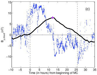
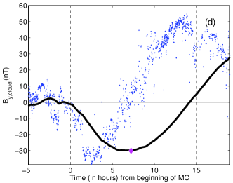
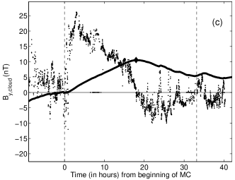
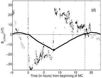
The observed magnetic field in an MC can be expressed in this local frame, transforming the observed components ($B_{x}$, $B_{y}$, $B_{z}$) with a rotation matrix to ($B_{x,\rm cloud}$, $B_{y,\rm cloud}$, $B_{z,\rm cloud}$). In particular, for $p=0$ and an MC described by a cylindrical magnetic configuration, i.e. $\@vec{B}(r)=B_{z}(r)\hat{z}+B_{\phi}(r)\hat{\phi}$, we have $\hat{x}_{\rm cloud}=\hat{r}$ and $\hat{y}_{\rm cloud}=\hat{\phi}$ when the spacecraft leaves the cloud. In this particular case, the magnetic field data will show: $B_{x,\rm cloud}=0$, a large and coherent variation of $B_{y,\rm cloud}$ (with a change of sign), and an intermediate and coherent variation of $B_{z,\rm cloud}$, from low values at one cloud edge, with the largest value at its axis and returning to low values at the other edge.

More generally, the local system of coordinates is especially useful when $p$ is small compared to the MC radius ($R$) since the direction of the MC axis can be found using a fitting method or applying the minimum variance (MV) technique to the normalized time series of the observed magnetic field (e.g. Dasso et al., 2006, and references therein). In particular, from the analysis of a set of cylindrical synthetic MCs, Gulisano et al. (2007) found that the normalized MV technique provides a deviation of the real orientation of the main MC axis of less than $10^{\circ}$ even for $p$ as large as $50\%$ of the MC radius.

2.3 Definition of the MC boundaries

As the first step of an iterative process, we choose the MC boundaries reported in the literature, and perform a normalized minimum variance analysis to find the local frame of the MC. We then analyze the magnetic field components in the local frame, and redefine the boundaries of each MC, according to the expected typical behavior of the axial field ($B_{z,cloud}$, having its maximum near the center and decreasing toward the MC boundaries), the azimuthal field ($B_{y,cloud}$, maximum at one of the borders, minimum at the other one and changing its signs near the cloud center), and $B_{x,cloud}$, which is expected to be small and with small variations (see Gulisano et al., 2007). Moreover, in the MC frame it is easier to differentiate the SW and MC sheath magnetic field, which is fluctuating, from the MC field, which has a coherent and expected behaviour for the three field components. We then moved the borders in order to reach these properties of the local field components, and performed the same procedure iteratively to find an improved orientation, using several times the minimum variance technique. We applied this procedure to each MC of our sample.

Table 1: List of MC events.

S/C	$T_{c}$	Group	$\Delta V_{x}/(t_{out}-t_{in})$		$\zeta$
	d-m-y h:m (UT)		km s-1 h-1
H1	07-Jan-1975 10:39	N	11.	1	1.	0
H1	04-Mar-1975 21:37	N	8.	75	0.	63
H1	02-Apr-1975 09:00	P	-6.	84	-1.	1
H1	05-Jul-1976 14:20	P	0.	15	0.	04
H1	30-Jan-1977 03:18	P	6.	13	1.	4
H1	31-Jan-1977 00:26	P	3.	68	0.	75
H1	20-Mar-1977 01:13	P	4.	28	0.	52
H1	09-Jun-1977 01:22	N	4.	26	0.	86
H1	09-Jun-1977 10:33	P	3.	71	0.	9
H1	28-Aug-1977 21:36	P	0.	92	0.	25
H1	26-Sep-1977 03:45	N	14.	8	0.	97
H1	01-Dec-1977 20:15	P	-0.	6	-0.	11
H1	03-Jan-1978 19:21	N	14.	1	0.	83
H1	16-Feb-1978 07:25	N	7.	66	1.	5
H1	02-Mar-1978 12:33	N	4.	99	0.	89
H1	30-Dec-1978 01:50	N	12.	4	1.	1
H1	28-Feb-1979 10:13	N	5.	7	0.	78
H1	03-Mar-1979 18:49	N	5.	51	0.	58
H1	28-May-1979 23:07	p	-4.	57	-0.	37
H1	01-Nov-1979 09:09	P	2.	62	0.	5
H1	22-Mar-1980 21:25	P	7.	78	2.	0
H1	10-Jun-1980 20:31	P	-6.	27	-0.	62
H1	20-Jun-1980 05:47	P	4.	24	0.	48
H1	23-Jun-1980 12:25	P	3.	6	0.	75
H1	27-Apr-1981 11:55	N	11.	9	1.	3
H1	11-May-1981 23:30	N	21.	6	1.	0
H1	27-May-1981 05:43	N	6.	83	0.	89
H1	19-Jun-1981 05:05	N	25.	5	0.	75
H2	06-Jan-1978 06:50	N	6.	97	0.	84
H2	30-Jan-1978 05:02	P	11.	7	1.	2
H2	07-Feb-1978 13:45	N	2.	42	0.	68
H2	17-Feb-1978 02:32	N	3.	23	0.	8
H2	24-Apr-1978 11:54	P	15.	4	1.	0
H1		all	6.	2 $\pm$ 7.3	0.	66 $\pm$ 0.65
H1		P	1.	3 $\pm$ 4.5	0.	39 $\pm$ 0.81
H1		N	11.	1 $\pm$ 6.3	0.	94 $\pm$ 0.25
H2		all	8.	0 $\pm$ 5.6	0.	90 $\pm$ 0.19
H2		P	13.	6 $\pm$ 2.6	1.	09 $\pm$ 0.13
H2		N	4.	2 $\pm$ 2.4	0.	77 $\pm$ 0.08
Both		all	6.	5 $\pm$ 7.	0.	70 $\pm$ 0.61
Both		P	2.	9 $\pm$ 6.	0.	48 $\pm$ 0.79
Both		N	10.	0 $\pm$ 6.4	0.	91 $\pm$ 0.23

The first column in Table 1 indicates the spacecraft (Helios 1 or Helios 2), $T_{c}$ in the second column is the time for the observation of the MC center (or for the minimum approach distance). The MCs are separated in two groups: perturbed (P) and non-perturbed (N) by a fast SW stream. $\Delta V_{x}/(t_{out}-t_{in})$ is minus the fitted slope of the temporal velocity profile (see, Eq. 2) and $\zeta$ is the non-dimensional expansion coefficient (Eq. 8). $\Delta V_{x}/(t_{out}-t_{in})<0$ means observed compression of the MC. The average values and the standard deviations are given at the bottom.

2.4 Characterization of the MC expansion

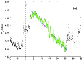
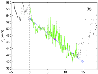
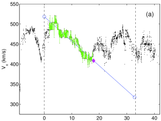
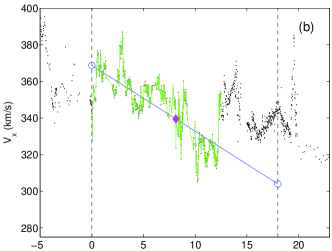
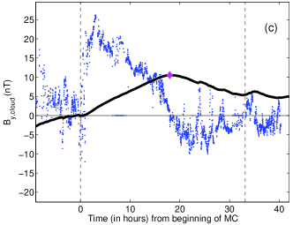
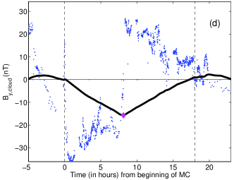
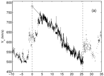
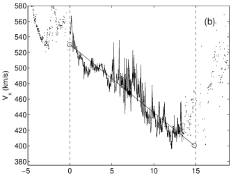
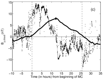
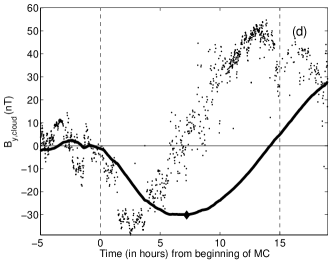
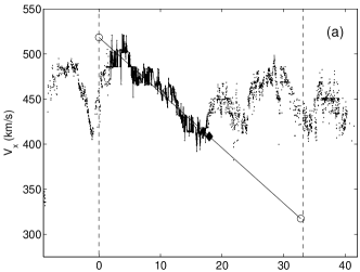
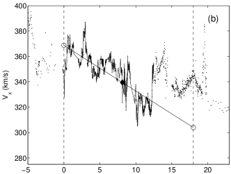
Most MCs have a higher velocity in their front than in their back, showing that they are expanding magnetic structures in the SW. About half of the studied MCs have well defined linear profile $V_{x}(t)$ (Fig. 1a,b), while for the other half, $V_{x}(t)$ is nearly linear only in a part of the MC which includes the MC center (Fig. 2a,b). The distortions of $V_{x}(t)$ are more frequently due to an overtaking faster SW flow in the back of the MC.

We split the data set in two groups: non-perturbed MCs for cases where the velocity profile presents a linear trend in more than $75$% of the full size of the MC and perturbed MCs for cases where this is not satisfied. There are almost as many perturbed as non-perturbed MCs, considering data from each spacecraft separately and both of them together. The measured temporal profile $V_{x}(t)$ is fitted using a least square fit with a linear function of time,

$$V_{x,\rm fit}(t)=V_{\rm o,fit}+({\mathrm{d}}V_{x}/{\mathrm{d}}t)_{\rm fit}\leavevmode\nobreak\ t\,,$$ (1)

where $({\mathrm{d}}V_{x}/{\mathrm{d}}t)_{\rm fit}$ is the fitted slope of the linear function. We always keep the fitting range inside the MC, but restrict it to the most linear part of the observed profile. This choice minimizes the effect of the interacting flows (but it does not fully remove it, since a long term interaction can, a priori, change the expansion rate of the full MC).

The linear fit is used to define the velocities $V_{x,\rm fit}(t_{in})$ and $V_{x,\rm fit}(t_{out})$ at the MC boundaries (Sect. 2.3). Then, we define the full expansion velocity of an MC as:

$$\Delta V_{x}=V_{x,\rm fit}(t_{in})-V_{x,\rm fit}(t_{out})\,.$$ (2)

For non-perturbed MCs, $\Delta V_{x}$, is very close to the observed velocity difference $V_{x}(t_{in})-V_{x}(t_{out})$, see e.g. upper panels of Fig. 1. For perturbed MCs, this procedure minimizes the effects of the perturbations entering the MC. Then, the expansion velocity is defined consistently for the full set of MCs.

Figure 3: The panels a-d show the correlation analysis between proxies for MC expansion with different physical quantities. The MCs are separated in two groups: perturbed (empty square symbol) and non-perturbed (filled circle symbol). The straight lines are the result of a least square fit for perturbed (dashed line), non-perturbed (thin continuous line), and for both set of MCs in the list of events shown in Table 1 (thick continuous line). $\Delta V_{x}$ is defined by Eq. (2), $\Delta t=t_{\rm out}-t_{\rm in}$, $V_{c}$ is the velocity of the MC center (or at the closest approach distance), and $D$ is the distance to the Sun. The fitted values and the obtained correlation coefficient ($r$) are included as insets, considering the different groups. More significant correlation is present for the non-perturbed cases (A color version is available in the electronic version).

2.5 MC size

From the determination of the boundaries described above, we can estimate the size, $S$, of the flux rope along $\hat{x}$ (the Sun-Spacecraft direction). $S$ is computed as the time duration of observation of the MC multiplied by the MC velocity at the center of the structure (see end of section  2.7).

We perform a linear least square fit in log-log plots of $S$ as a function of the distance to the Sun ($D$). As expected, the size has a clear dependence with $D$:

$$S_{\rm full\ set} = (0.23\pm 0.01)\leavevmode\nobreak\ D^{0.78\pm 0.12}$$

$$S_{\rm non-perturbed} = (0.32\pm 0.02)\leavevmode\nobreak\ D^{0.89\pm 0.15}$$ (3)

$$S_{\rm perturbed} = (0.16\pm 0.01)\leavevmode\nobreak\ D^{0.45\pm 0.16}\,,$$

where $S$ and $D$ are in AU. Our results are compatible within the error bars with previous studies:

$$d_{\rm Bothmer} = (0.24\pm 0.01)\leavevmode\nobreak\ D^{0.78\pm 0.10}$$

$$S_{\rm Liu} = (0.25\pm 0.01)\leavevmode\nobreak\ D^{0.92\pm 0.07}$$ (4)

$$S_{\rm Wang} = \leavevmode\nobreak\ 0.19\qquad\quad\,\,\leavevmode\nobreak\ D^{0.61}$$

$$d_{\rm Leitner} = (0.20\pm 0.02)\leavevmode\nobreak\ D^{0.61\pm 0.09}\,,$$

where $d$ is an estimation of the true diameter of the MC. Our results are closer to Bothmer & Schwenn (1998) and Liu et al. (2005) who analyzed MCs and ICMEs, respectively. The larger difference is between our results and the last two ones while they are based on the most different sets, as follows. Wang et al. (2005) studied a large set of ICMEs defined only by a measured temperature lower by a factor of 2 than expected in the SW with the same speed (e.g., Richardson & Cane, 2004). This set included MCs, but it is dominated by non-MC ICMEs. Conversely, Leitner et al. (2007) analyzed only MCs, with a strict classical definition. They fitted the magnetic field observations with a classical cylindrical linear force-free field, then they found the impact parameter and the orientation of the MC axis to estimate the true diameter, $d$, of the MCs. So the selected events and the method of Wang et al. and Leitner et al. are noticeably different. We also note that Leitner et al. (2007) found a larger exponent, $1.14\pm 0.44$, when they restrict their data to $D\leq 1$ AU. This indicates that the relation is not strictly a power-law and this could be the main origin of the different results (which are so dependent on the distribution of events with solar distance in the selected sets).

Figure 4: Panels a-d show the correlation analysis that tests for the dependence of the non-dimensional expansion factor $\zeta$ (Eq. 8) as a function of other parameters. Perturbed and non-perturbed MCs are represented as in Fig. 3. $S_{\rm corrected\leavevmode\nobreak\ to\leavevmode\nobreak\ 1\leavevmode\nobreak\ AU}$ and $<B>_{\rm corrected\leavevmode\nobreak\ to\leavevmode\nobreak\ 1\leavevmode\nobreak\ AU}$ are normalized to 1 AU using the size and field strength dependence on the distance, according to the relationship given in Eq. (9). (A color version is available in the electronic version).

2.6 Magnetic field strength

Another important characteristic of MCs is their magnetic field strength. We define the average field $<B>$ within each MC and proceed as above with $S$. $<B>$ has an even stronger dependence upon distance:

$$<B>_{\rm full\ set} = (10.9\,\pm\ 0.4)\quad D^{-1.85\pm 0.07}$$

$$<B>_{\rm non-perturbed} = (11.4\,\pm\ 0.5)\quad D^{-1.85\pm 0.11}$$ (5)

$$<B>_{\rm perturbed} = (10.4\,\pm\ 0.6)\quad D^{-1.89\pm 0.10}\,,$$

where the units of $<B>$ and $D$ are nT and AU respectively. Our results have a stronger dependence on $D$ than previous results:

$$<B>_{\rm Liu} = (7.4\pm 0.4)\leavevmode\nobreak\ D^{-1.40\pm 0.08}$$

$$<B>_{\rm Wang} = \leavevmode\nobreak\ 8.3\qquad\,\,\,\,\,\,D^{-1.52}$$ (6)

$$<B>_{\rm Leitner} = (19\pm 1.4)\ \leavevmode\nobreak\ D^{-1.30\pm 0.09}\,.$$

Again the strongest difference exists between our results and the ones of Leitner et al. (2007). The origin of this difference is expected to be the same as for the size. Indeed for $D\leq 1$ AU, Leitner et al. (2007) found a more negative exponent, $-1.64\pm 0.4$, closer to our results, as ocurred for the size.

The typical expansion speed in MCs is of the order of half the Alfvén speed (e.g., Klein & Burlaga, 1982). In our studied set of MCs, we have also found that the expansion speed was lower than the Alfvén speed [not shown]. This is a necessary condition to expect that the magnetic field evolves globally, adapting its initial magnetic field during its expansion, because the Alfvén speed is the velocity of propagation of information through the magnetic structure.

2.7 MC center and translation velocity

Following Dasso et al. (2006), we define the accumulative flux per unit length $L$ (along the MC axial direction):

$$\frac{F_{y}(t_{1},t_{2})}{L}=\int_{t_{1}}^{t_{2}}B_{y,cloud}(t^{\prime})\leavevmode\nobreak\ V_{x,cloud}(t^{\prime})\leavevmode\nobreak\ {\mathrm{d}}t^{\prime}\,.$$ (7)

Here we neglect the evolution of the magnetic field during the spacecraft crossing period (so also the “aging” effect, see Dasso et al., 2007). The set of field lines, passing at the position of the spacecraft at $t_{1}$, with the hyphotesis of symmetry of translation along the main axis, defines a magnetic flux surface, which is wrapped around the flux rope axis. Then, any magnetic flux surface will be crossed at least twice by the spacecraft, once at $t_{1}$ and once at $t_{2}$ defined by $F_{y}(t_{1},t_{2})=0$. Then, this property of $F_{y}(t_{1},t_{2})$ permits us to associate any out-bound position, within the flux rope, to its in-bound position belonging to the same magnetic-flux surface. The global extremum of $F_{y}(t_{1},t)$, for $t_{1}$ having a fixed value, locates the position where the spacecraft trajectory has the closest approach distance to the MC axis (MC center). This position can also be found directly from $B_{y,cloud}(t)$, where $B_{y,cloud}$ crosses zero. Nevertheless, using the integral quantity $F_{y}$ has the advantage of decreasing the fluctuations and of outlining the global extremum, compared to the local extrema (see lower panels of Figs. 1 and 2).
The velocity at the MC center ($V_{c}$) is computed from the fitted linear regression Eq. (1) evaluated at the time when the spacecraft reaches the MC center.

3 Expansion rate of MCs

3.1 Correlation involving the expansion velocity

From here on, we classify the MCs belonging to the full set of events, according to the quality of their velocity and magnetic observations. If they were too noisy or with a lot of data gaps, we exclude them from the following study, keeping only those MCs with relatively good quality (listed in Table 1).

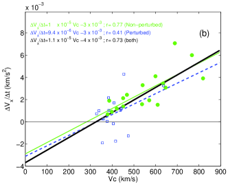
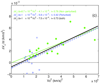
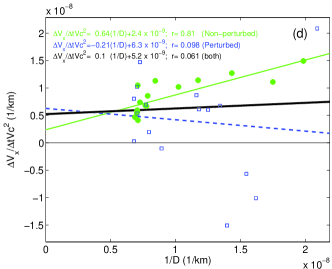
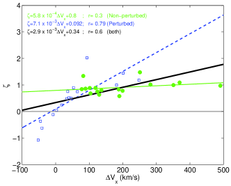
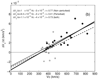
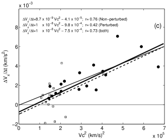
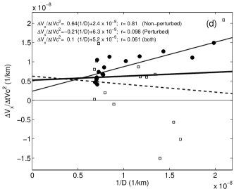
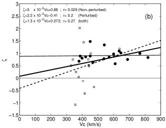
$\Delta V_{x}$, as defined by Eq. (2), characterizes the expansion speed of the crossed MC. However, as outlined in Sect. 1, $\Delta V_{x}$ is expected to be strongly correlated with the MC size, so that it does not express directly how fast a given parcel of plasma is expanding in the MC. We therefore define below, after a few steps, a better measure of the expansion rate. The size of an MC is proportional to $\Delta t=t_{\rm out}-t_{\rm in}$ and to $V_{c}$. Fig. 3a shows a clear positive correlation between $\Delta V_{x}$ and $\Delta t$. Moreover the least square fit of a straight line for the full set of MCs gives a fitted curve passing in the vicinity of the origin (within the uncertainties present on the slope). This affine correlation is then removed by computing $\Delta V_{x}/\Delta t$. This quantity also shows, as expected, a positive correlation with $V_{c}$ (Fig. 3b), but differently above, the fitted straight line stays far from the origin, so we cannot simply remove the correlation by dividing $\Delta V_{x}/\Delta t$ by $V_{c}$. However, its dependence on $V_{c}^{2}$ brings the fitted straight line close enough to the origin (within the uncertainties of the fit, Fig. 3c) so that $\Delta V_{x}/(\Delta tV_{c}^{2})$ is a meaningful quantity. These correlations are present for both groups of MCs, but they are much stronger for non-perturbed MCs (Fig. 3b,c). Other correlations have being attempted with the above methodology. Either there is no significant correlation, or the fitted curve passes far from the origin. There is still the exception that $\Delta V_{x}/(\Delta tV_{c}^{2})$ has an affine correlation with $1/D$ for non-perturbed MCs (Fig. 3d).

3.2 Non-dimensional expansion rate

The above empirical correlation analysis suggests that we can define the non-dimensional expansion rate as the quantity:

$$\zeta=\frac{\Delta V_{x}}{\Delta t}\frac{D}{V_{c}^{2}}\,.$$ (8)

The first steps were to remove the MC size dependence, while the last step could be further justified by the need to have a non-dimensional coefficient. Finally, it is remarkable that the correlation analysis of the MC data leads to the definition of the same variable, $\zeta$, as the theoretical analysis of Démoulin & Dasso (2009).

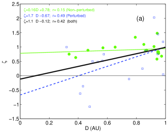
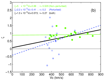
We next verify that $\zeta$ is no longer dependent on $\Delta t$, $V_{c}$, $D$ or some combination of them. Figures 4a,b show two examples of this exploration. Indeed, the non-perturbed MCs show almost no correlation, while there are still some correlations when the perturbed MCs are considered. Figure 4b also shows that even for slow MCs (see Sect. 1), the non-dimensional expansion rate ($\zeta$) is not correlated with $V_{c}$.

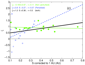
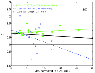
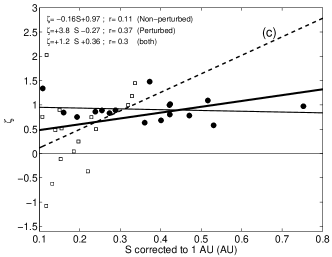
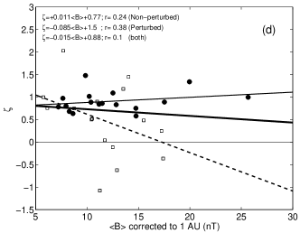
Still, does $\zeta$ depend on the properties of the MC considered? To test this we first need to remove the distance dependence on $S$ and $<B>$, found in Sect. 2.5 and 2.6, by defining values at a given solar distance (here taken at 1 AU). We use:

$$S_{\rm corrected\leavevmode\nobreak\ to\leavevmode\nobreak\ 1\leavevmode\nobreak\ AU} = S\leavevmode\nobreak\ D^{-0.8}$$

$$<B>_{\rm corrected\leavevmode\nobreak\ to\leavevmode\nobreak\ 1\leavevmode\nobreak\ AU} = <B>\leavevmode\nobreak\ D^{+1.8}\,.$$ (9)

We find that there is no significant correlation between $\zeta$ and $S_{\rm corrected\leavevmode\nobreak\ to\leavevmode\nobreak\ 1\leavevmode\nobreak\ AU}$, as well as between $\zeta$ and $<B>_{\rm corrected\leavevmode\nobreak\ to\leavevmode\nobreak\ 1\leavevmode\nobreak\ AU}$ for the non-perturbed MCs (Fig. 4c,d). Taking other exponents, in the vicinity $(\pm 0.4)$ of the exponents used in Eq. 9, we also find very low correlation coefficients, in the ranges [0.08,0.15] for $S_{\rm corrected\leavevmode\nobreak\ to\leavevmode\nobreak\ 1\leavevmode\nobreak\ AU}$ and [0.15,0.29] for $<B>_{\rm corrected\leavevmode\nobreak\ to\leavevmode\nobreak\ 1\leavevmode\nobreak\ AU}$.

Figure 5: Perturbed and non-perturbed MCs have a remarkably different behavior of $\zeta$ when they are plotted as a function of $\Delta V_{x}$. The drawing convention is the same as in Figs. 3,4 (A color version is available in the electronic version).

Figure 6: Cartoon of a possible evolution of the size of the MC with the helio-distance, showing the expected global expansion (thick solid line), an example of a non-perturbed MC (thin solid) and a perturbed MC (dashed line). (A color version is available in the electronic version).

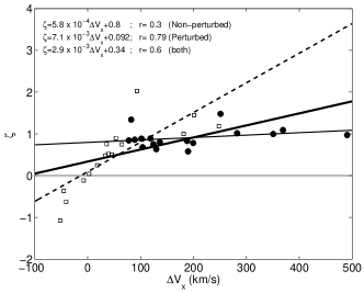
3.3 Expansion of non-perturbed MCs

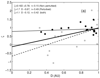
Perturbed and non-perturbed MCs have a remarkable different behavior of $\zeta$ as a function of $\Delta V_{x}$ (Fig. 5). While for non-perturbed MCs the correlations have been removed, the perturbed ones have $\zeta$ well correlated with $\Delta V_{x}$ ($r=0.79$).

To explain the different behavior of $\zeta$ let us take into account that the dependence of the size on the heliocentric distance is of the form (as observed from several statistical studies, Eqs. 3-4):

$$S=S_{0}(D/D_{0})^{m}\,,$$ (10)

where $S_{0}$ is the reference size at the distance $D_{0}$. Its physical origin is the approximate pressure balance between the MC and the surrounding SW (Démoulin & Dasso, 2009, see Sect. 3.5). This physical driving of the expansion is expected to induce a smooth expansion so that the size of an individual MC closely follows Eq. (10). Then, for non-perturbed MCs, we can differentiate Eq. (10) with time to derive the expansion velocity $\Delta V_{x}$:

$$\Delta V_{x}\approx\frac{dS}{dt}\approx\frac{dS}{dD}\frac{dD}{dt}\approx m\frac{S}{D}\leavevmode\nobreak\ V_{c}\,.$$ (11)

Then, the non-dimensional expanding rate of Eq. (8) is:

$$\zeta_{\rm non-perturbed}=\frac{\Delta V_{x}}{\Delta t}\frac{D}{V_{c}^{2}}\approx m\,.$$ (12)

This implies that $\zeta$ is independent of the size and the velocity of the MC as well as its distance from the Sun and its global expansion rate $\Delta V_{x}$, in agreement with our results (Figs. 4,5). It also implies that the velocity measurements across a given MC permits to estimate the exponent $m$ in Eq. (10). Indeed the values of $m$ deduced from the statistical study of MC size versus distance (Eq. 3) are in agreement with the mean value found independently with the velocity measurements (Fig. 5, Table 1).

3.4 Expansion of perturbed MCs

For perturbed MCs, the estimation of $\zeta$ both from the size evolution with distance and from the measured velocity still gives consistent estimations (Eq. 3, Table 1). However, the mean value of $\zeta$ is lower ($\zeta\approx m\approx 0.45$) than for non-perturbed MCs ($\zeta\approx m\approx 0.8$). More important, $\zeta$ has a much larger spread for perturbed than non-perturbed MCs (by a factor $\approx 4$ larger). Such a larger dispersion of $\zeta$ is expected to be the result of the variable physical parameters (such as ram pressure) of the overtaking streams, and also because the interaction is expected to be in a different temporal stage for different perturbed MCs (ranging from the beginning to the end of the interaction period).

The effect of an overtaking stream is simply to compress the MC (at first thought), so MCs perturbed by this effect are expected to have a lower $\zeta$ than non-perturbed MCs. This is true in average, but there is a significant fraction (5/16) of perturbed MCs that are in fact expanding faster than the mean of non-perturbed MCs. The largest $\zeta$ is also obtained for a perturbed MC. Moreover, $\zeta$ for perturbed MCs still has a good correlation with $\Delta V_{x}$, opposite to the result obtained for non-perturbed MCs (Fig. 5). Why do perturbed MCs have these properties?

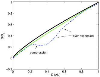
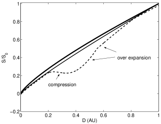
When an MC is overtaken by a fast SW stream, it is compressed by the ram, plasma and magnetic pressure of the overtaking stream, so its size increases less rapidly with solar distance (than without interaction). If the interaction is strong enough, this can indeed stop the natural expansion and create an MC in compression, as in the 3 cases present in Table 1, where $\Delta V_{x}<0$. A sketch of such evolution is given in Fig. 6. However, this interaction will not last for a long period of time since the overtaking stream can overtake the flux rope from both sides. As the total pressure in the back of the MC decreases, the expansion rate of the MC increases. Indeed, its expansion rate could be faster than the typical one for non-perturbed MCs, as follows. The compression has provided an internal pressure that is stronger than the surrounding SW total pressure. Then, when the extra pressure of the overtaking stream has significantly decreased, the MC has an over-pressure compared to the surrounding SW, so it expands faster than usual i. e., an overexpansion, see Gosling et al. (1995). Indeed, the flux rope is expected to evolve towards the expected size that it would have achieved without the overtaken SW flow.

So, depending on which time the MC is observed in the interaction process, a perturbed MC can expand slower or faster than without interaction (Fig. 6). This explains the dispersion of $\zeta$ found for perturbed MCs, but also the presence of some MCs with faster expansion than usual.

In the case of perturbed MCs, their sizes still follow Eq. (10) on average (as shown by Eq. 3), but it has no meaning to apply this law locally to a given MC. In particular, we cannot differentiate Eq. (10) with time to get an estimation of the local expansion velocity of a perturbed MC (so we cannot write Eq. 11). Rather we can use Eq. (10) only to have an approximate size $S$ in the expression of $\zeta$:

$$\zeta_{\rm perturbed}=\frac{\Delta V_{x}}{S}\frac{D}{V_{c}}\approx\frac{\Delta V_{x}{D_{0}}^{m}D^{1-m}}{S_{0}V_{c}}\,.$$ (13)

The dependence of $D^{1-m}\approx D^{0.5}$ is relatively weak, but still present (Fig. 4a). $\zeta$ also has a dependence on $V_{c}$, but the range of $V_{c}$ within the studied perturbed group is very limited to derive a reliable dependence from the observations (Fig. 4b), and, moreover, there is a dependence on $S_{0}$ that we cannot quantify. It remains that the strongest correlation of $\zeta$ is with $\Delta V_{x}$ (Fig. 5). Indeed, for perturbed MCs, $\zeta$ strongly reflects their local expansion behavior, so that $\zeta$ is strongly correlated to $\Delta V_{x}$.

Figure 7: Log-log plots of the SW total pressure and its components as a function of the solar distance. The solid line shows the least square straight line fitted to the total pressure as computed from the points marked with circles. The total pressure in the SW decreases as $P_{sw}(D)=P_{0}D^{-2.9}$ (A color version is available in the electronic version).

3.5 Physical origin of MC expansion

The main driver of MC expansion is the rapid decrease of the total SW pressure with solar distance (Démoulin & Dasso, 2009). Other effects, such as the internal over-pressure, the presence of a shock, as well as the radial distribution and the amount of twist within the flux rope have a much weaker influence on the expansion. This result was obtained by solving the MHD equations for flux ropes having various magnetic field profiles, and with ideal MHD or fully relaxed states (minimizing magnetic energy while preserving magnetic helicity). Within the typical SW conditions, they have shown that any force-free flux rope will have an almost self similar expansion, so a velocity profile almost linear with time as observed by a spacecraft crossing an MC (e.g. Figs. 1,2). They also relate the normalized expansion rate $\zeta$ to the exponent $n_{P}$ of the total SW pressure as a function of the distance $D$ to the Sun (defined by $p\propto D^{-n_{P}}$) as $\zeta\approx n_{P}/4$.

Here we further test the above theory with the MCs analyzed in this paper, by comparing the value obtained for $\zeta$ with the value of $n_{P}$ obtained from previous studies of the SW.

According to Mariani & Neubauer (1990), from fitting a power law to observations of the field strength in the inner heliosphere according to $B=B_{0}(D/D_{0})^{-n_{B}}$, a global decay law is obtained with $n_{B}=1.6\pm 0.1$ ($B_{0}=3.8\pm 0.2$ nT at $D_{0}=1$AU) from Helios 1, and $n_{B}=1.8\pm 0.1$ ($B_{0}=3.3\pm 0.2$ nT at $D_{0}=1$AU) from Helios 2.

For the proton density ($N_{p}=N_{p,0}(D/D_{0})^{-n_{N}}$) we consider a density of $N_{0}=7\pm 4$ cm^-3 at 1 AU (averaging slow and fast SW according to Schwenn, 2006) and $n_{N}=2$ (corresponding to the 2D expansion for the stationary SW with constant radial velocity).

According to Schwenn (2006) and Totten et al. (1995), it is possible to represent a typical dependence of the proton temperature ($T_{p}$) upon $D$ as approximately $T_{p}=T_{p,0}(D/D_{0})^{-n_{T_{p}}}$ with $n_{T_{p}}=1.0\pm 0.1$ ($T_{p,0}=(1.3\pm 1.0)\times 10^{5}$K at $D_{0}=1$AU).

For electron temperature ($T_{e}=T_{e,0}(D/D_{0})^{-n_{T_{e}}}$) we follow Marsch et al. (1989), in particular their results for the ranges of velocities (300-500) km/s to better represent the typical conditions of the SW. For the velocity range (300-400) km/s, Marsch et al. (1989) found $T_{e,0}=(1.3\pm 0.4)\times 10^{5}$ K and $n_{T_{e}}=0.5\pm 0.1$; for the velocity range (400-500) km/s, $T_{e,0}=(1.4\pm 0.4)\times 10^{5}$ K and $n_{T_{e}}=0.4\pm 0.1$. For electrons we then consider mean temperature averaged over these two ranges of SW speeds.

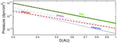
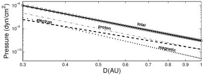
The partial pressures (magnetic, proton, and electron) are shown in Fig. 7. Neglecting the small effect of the $\alpha$ particles, the total pressure in the SW ($P_{SW}$) is: $P_{SW}=P_{B}+P_{p}+P_{e}$. We then propose that the total pressure also follows a power law ($P_{SW}=P_{0}D^{-n_{P}}$) and fit this power law to $P_{SW}(D_{i})$. Then, we fit $P_{SW}$ with a power law ($P_{0}D^{-n_{P}}$). The sum of different power laws is generally not a power law, however in the present case we still find a total pressure which is very close to a power law since the magnetic and plasma pressures have similar exponents. This also implies that the exponent found, $n_{P}=2.91\pm 0.31$, has a low sensitivity to the plasma $\beta$ and the relative pressure contribution of the electrons and protons.

Using the result of Démoulin & Dasso (2009) that $\zeta\approx n_{P}/4$ for force-free flux rope, we found $\zeta=0.73\pm 0.08$, in full agreement, within the error bars, with $\zeta$ found from velocity measurement in non-perturbed MCs (Table 1). This further demonstrates that MC expansion is mainly driven by the decrease of the surrounding SW total pressure with solar distance. The main departure from this global evolution is due to the presence of overtaking flows.

4 Summary and discussion of main results

MCs have a specific magnetic configuration, forming flux ropes which expand in all directions, unlike the almost 2D expansion of the surrounding SW. But how fast do they expand? Is the expansion rate specific for each MC or is there a common expansion rate? What is the role of the surrounding SW? Finally, what is the main driver of such 3D expansion?

In order to answer these questions we have re-analyzed a significant set of MCs observed by both Helios spacecrafts. In order to better define the MC extension, we first analyzed the magnetic data, finding the direction of the flux rope axis, and then we rotated the magnetic data in the MC local frame. This step is important to separate the axial and ortho-axial field components since they have very different spatial distributions in a flux rope, and since we then can use the magnetic flux conservation of the azimuthal component as a constraint on the boundary positions (e.g., as done in Dasso et al. (2006); Steed et al. (2008)). Then, in the local MC frame, we can better define the boundaries of the MC.

The observed velocity profile typically has a linear variation with time, with a larger velocity in front than in the back of the MC. This is a clear signature of expansion. On top of this linear trend, fluctuations of the velocity are relatively weak, with the most noticeable exception occurring when an overtaking fast stream is observed in the back of the MC. Such fast flow can enter the MC, removing the linear temporal trend. We consider these overtaken MCs in a separate group as perturbed MCs (Fig. 2). We exclude from the analysis the MCs where the overtaking flow was extending more than half the MC size and MCs where the data gaps were too large. The remaining MCs are classified as non-perturbed, even if some of them have weak perturbations in their velocity profiles. These perturbations are filtered by considering only the major part of the velocity profile where the profile is almost linear with time (Fig. 1).

The group of non-perturbed MCs has a broad and typical range of sizes and magnetic field strengths ($\approx[0.1,0.75]$ AU and $\approx[7,25]$ nT respectively when rescaled at 1 AU). They also have a broad range of expansion velocities ($\approx[80,500]$ km/s). Such a range of expansion velocity cannot be explained by the range of observing distances, ($D$ in $[0.3,1]$ AU), since the expansion velocity decreases only weakly within this range of $D$. However, we found that the expansion velocity is proportional to the MC size. By further analyzing the correlation between the observed expansion velocity and other measured quantities, such as the MC velocity, we empirically defined a non-dimensional expansion coefficient $\zeta$ (Eq. 8). For the non-perturbed MCs, $\zeta$ is independent of all the other characteristics of the MCs (such as size and field strength). Moreover, this empirical definition of $\zeta$, obtained by removing the correlation in the data between the expansion rate and other quantities, finally defines the same $\zeta$ quantity as the one defined from theoretical considerations by Démoulin et al. (2008). We conclude that $\zeta$ characterizes the expansion rate of non-perturbed MCs.

For the non-perturbed MCs, we found that $\zeta$ is confined to a narrow interval: $0.91\pm 0.23$. This is consistent with the result obtained at 1 AU for a set of 26 MCs observed by Wind and ACE (Démoulin et al., 2008). Indeed, we found that $\zeta$ is independent of solar distance (within $[0.3,1]$ AU) in the Helios MCs.

What is the origin of this common expansion rate of MCs? Démoulin & Dasso (2009) have shown theoretically that the main origin of MC expansion is the decrease of the total SW pressure with solar distance $D$. With a SW pressure decreasing as $D^{-n_{P}}$, they found that $\zeta\approx n_{P}/4$ independently of the magnetic structure of the flux rope forming the MC. In the present work, we re-analyzed the total SW pressure variation with $D$, revising previous studies that also analyzed Helios data (Mariani & Neubauer, 1990; Schwenn, 2006; Totten et al., 1995; Marsch et al., 1989). We found $n_{P}=2.91\pm 0.31$, which implies $n_{P}/4=0.73\pm 0.08$, in agreement with our estimation of $\zeta$ from the measured velocity in MCs. We then confirm that the fast decrease of the total SW pressure with solar distance is the main cause of the MC expansion rate.

For MCs overtaken by a fast SW stream (or by another flux rope on its back, e.g. Dasso et al. (2009)), we minimize its importance in the estimation of the MC expansion rate by considering only the part of the velocity profile which is nearly linear with time. Still, the mean computed $\zeta$ for perturbed MCs is significantly lower than the mean value for non-perturbed MCs, showing that the overtaking flows have a more global effect on MCs (than the part where the velocity profiles significantly depart from the linear temporal behavior). A lower expansion rate is a natural consequence of the compression induced by the overtaking flow.

More surprising, some perturbed MCs are found to expand faster (larger $\zeta$) than non-perturbed MCs. We conclude that such MC are probably observed after the main interaction phase with the overtaking flow, so that they expand faster than usual in order to sustain an approximate pressure balance with the surrounding SW (Fig. 6). More precisely, as the overtaking flow disappears from the back of the MC, the MC is expected to tend towards the size that it would have reached without the interaction with the fast stream. Since it was compressed, it is expanding faster than usual to return to its expected size in a normal SW.

5 Conclusions

Our present results confirm and extend our previous work on the expansion of MCs. The non-dimensional expansion factor $\zeta$ (Eq. 8) gives a precise measure of the expanding state of a MC. In particular, it removes the size effect which could give the false impression that parcels of fluid in large MCs are expanding faster. The value of $\zeta$ in non-significantly perturbed MCs is clustered in a narrow range, independent of their magnetic structure, but determined by the pressure gradient of the surrounding SW. The mean value of $\zeta$ is also nearly the exponent of the solar distance for the MC size (determined from the analysis of MCs at different solar distances, section  2.5).

However, for perturbed MCs, $\zeta$ has a much broader range, a result linked to its proportionality to the local expansion velocity. So for perturbed MCs, $\zeta$ is a measure of the local expansion rate and of the importance of the overtaking stream (i.e., a quantification of the influence of the MC/stream interaction on the expansion of the MC).

Finally for non-perturbed MCs, $\zeta$ is independent of the solar distance in the inner heliosphere. Presently we do not know how far this result extends to larger distances, even if it is an expected result as long as the flux ropes still exist. This will be the subject of a future study.

Next pages: Color version of some figures (for the electronic version)

Figure 1: Examples of two analyzed MCs that are not significantly perturbed by a fast flow. The MC center was observed at 07-Jan-1975 10:39 and 04-Mar-1975 21:37 UT, for panels (a,c) and (b,d), respectively. The vertical dashed lines define the MC boundaries. (a,b) $V_{x}$ is the observed velocity component in the radial direction from the Sun, expressed in km per second. The straight line is the linear least square fit of the velocity in the time interval where an almost linear trend is present (where the observations are presented as a solid line). The linear fitting is extrapolated to the borders of the MC, which are marked with circles. (c,d) $B_{y}$ is the magnetic field component, in nT, both orthogonal to the MC axis and to the spacecraft trajectory, while the solid line represents $F_{y}$, which is the accumulated flux of $B_{y}$ (Eq. 7). The extremum of $F_{y}$ (proxy of the cloud center) is indicated with diamonds.

Figure 2: Examples of two analyzed MCs that are perturbed by a fast flow as seen in the upper panels. The MC center was observed at 30-Jan-1977 03:18 and 23-Jun-1980 12:25 UT, for panels (a,c) and (b,d), respectively. The external perturbations enter in a significant part of the MCs. The same quantities, as in Fig. 1, are shown.

Figure 3: The panels a-d show the correlation analysis between proxies for MC expansion with different physical quantities. MCs are separated in two groups: perturbed (empty square symbol) and non-perturbed (filled circle symbol). The straight lines are the result of a least square fit for perturbed (dashed line), non-perturbed (thin continuous line), and for both set of MCs in the list of events shown in Table 1 (thick continuous line). $\Delta V_{x}$ is defined by Eq. (2), $\Delta t=t_{\rm out}-t_{\rm in}$, $V_{c}$ is the velocity of the MC center (or at the closest approach distance), and $D$ is the distance to the Sun. The fitted values and the obtained correlation coefficient ($r$) are included as insets, considering the different groups. More significant correlation is present for the non-perturbed cases.

Figure 4: Panels a-d show the correlation analysis that tests for the dependence of the non-dimensional expansion factor $\zeta$ (Eq. 8) as a function of other parameters. Perturbed and non-perturbed MCs are represented as in Fig. 3. $S_{\rm corrected\leavevmode\nobreak\ to\leavevmode\nobreak\ 1\leavevmode\nobreak\ AU}$ and $<B>_{\rm corrected\leavevmode\nobreak\ to\leavevmode\nobreak\ 1\leavevmode\nobreak\ AU}$ are normalized to 1 AU using the size and field strength dependence on the distance, according to the relationship given in Eq. (9).

Figure 5: Perturbed and non-perturbed MCs have a remarkably different behavior of $\zeta$ when they are plotted as a function of $\Delta V_{x}$. The drawing convention is the same as in Figs. 3,4.

Figure 6: Cartoon of a possible evolution of the size of the MC with the helio-distance, showing the expected global expansion (thick solid line), an example of a non-perturbed MC (thin solid) and a perturbed MC (dashed line).

Figure 7: Log-log plots of the SW total pressure and its components as a function of the solar distance. The solid line shows the least square straight line fitted to the total pressure as computed from the points marked with circles. The total pressure in the SW decreases as $P_{sw}(D)=P_{0}D^{-2.9}$.