Caustic echoes from a Schwarzschild black hole

Abstract

We present the first numerical approximation of the scalar Schwarzschild Green function in the time domain, which reveals several universal features of wave propagation in black hole spacetimes. We demonstrate the trapping of energy near the photon sphere and confirm its exponential decay. The trapped wavefront passes through caustics resulting in echoes that propagate to infinity. The arrival times and the decay rate of these caustic echoes are consistent with propagation along null geodesics and the large $\ell$ limit of quasinormal modes. We show that the fourfold singularity structure of the retarded Green function is due to the well-known action of a Hilbert transform on the trapped wavefront at caustics. A twofold cycle is obtained for degenerate source-observer configurations along the caustic line, where the energy amplification increases with an inverse power of the scale of the source. Finally, we discuss the tail piece of the solution due to propagation within the light cone, up to and including null infinity, and argue that, even with ideal instruments, only a finite number of echoes can be observed. Putting these pieces together, we provide a heuristic expression that approximates the Green function with a few free parameters. Accurate calculations and approximations of the Green function are the most general way of solving for wave propagation in curved spacetimes and should be useful in a variety of studies such as the computation of the self-force on a particle.

I Introduction

A general technique to study the full response of a black hole to generic perturbations is to explore the Green function. While the Green function (aptly called the propagator) is simple in flat spacetime, it has a rich structure in curved spacetimes.

Recently, Ori discovered that the Green function in Schwarzschild spacetime displays a fourfold periodic structure Ori . This fourfold structure can be understood in terms of trapped null geodesics, similar to the classical interpretation of quasinormal mode ringing as energy leakage from the photon sphere Ames and Thorne (1968); Goebel (1972). At each half revolution along the trapped orbit, the trapped wavefront passes a caustic undergoing a transformation with a fourfold cycle. Ori investigated this cycle using a quasinormal mode expansion method. He also performed an acoustic experiment providing evidence for the structure of trapped signals through caustics.

The fourfold cycle has been formally analyzed in General Relativity for the first time by Casals, Dolan, Ottewill, and Wardell in Casals et al. (2009, 2010) in the example of Nariai spacetimes. Recently, Casals and Nolan developed a Kirchhoff’s integral representation of the Green function on Plebański–Hacyan spacetimes, confirming the appearance of the fourfold singularity structure in these black-hole models Casals and Nolan (2012). Going beyond toy models, Dolan and Ottewill discussed the Green function in Schwarzschild spacetime using large $\ell$ quasinormal mode sums Dolan and Ottewill (2011) based on their expansion method Dolan and Ottewill (2009). The essential singularity structure of the retarded Green function in arbitrary spacetimes has been discussed by Harte and Drivas Harte and Drivas (2012). They approximate the region of any spacetime near a null geodesic by a pp-wave spacetime in the Penrose limit. Their analysis implies, in particular, that the fourfold structure should be valid also in Kerr spacetimes.

Motivated by these theoretical studies and by Ori’s acoustic experiment, we perform a numerical experiment and analyze in detail the response of a black hole to compactly supported scalar perturbations. We describe the problem and our numerical setup in Sec. II. The main part of this paper (Sec. III) contains our results organized by scales, from the geometrical optics limit (short wavelength) to the curvature scale (long wavelength). After a qualitative description of the evolution of compactly supported wave packets in Sec. III.1, we discuss the propagation of the signal along null geodesics and the subsequent caustic echoes as measured by an observer at infinity (Sec. III.2). Wave propagation through caustics and the fourfold structure of the Green function is studied in Sec. III.3. We show that the fourfold structure is due to the action of a Hilbert transform at each passage through a caustic. In Sec. III.4 we present a twofold cycle for degenerate source-observer configurations and find an inverse power relation between energy magnification at caustics and the source scale. We argue that the trapping of energy near the black hole is the universal cyclic feature manifested in the Green function, not the number of the cycle (e.g., four or two). In Sec. III.5 we analyze the tail of the signal due to scattering off the background curvature, which dominates at late times implying that only a finite number of echoes can be observed even with ideal instruments. Putting these pieces together in Sec. III.6, we provide a heuristic expression for the Green function with a few free parameters. We present our findings, discuss the limitations of our method, and pose problems for future research in Sec. IV. The Appendixes complement the main text. The topics include hyperboloidal compactification for numerical simulations (Appendix A), the Schwarzschild Green function in the geometrical optics limit (Appendix B), and the Hilbert transform at caustics (Appendix C).

II The Setup

II.1 The problem description

The simplest model equation to describe essential features of wave propagation is the scalar wave equation

$$\Box\phi(x)=S(x)\,,$$ (1)

for a scalar field $\phi$ with source $S$ that depends on spacetime coordinates $x$. The wave operator, $\Box$, is written with respect to a background Schwarzschild metric. We set the source to

$$S(x)=\frac{1}{(2\pi\sigma^{2})^{2}}\exp\left(-\frac{\delta_{\mu\nu}(x^{\mu}-x^{\prime\mu})(x^{\nu}-x^{\prime\nu})}{2\sigma^{2}}\right),$$ (2)

where $\delta_{\mu\nu}$ is the four-dimensional Kronecker delta and $\sigma$ sets the scale for the width of the perturbation. The Gaussian source to the scalar wave equation is chosen to approximate the delta distribution because we are interested in the evolution of wavefronts and in the numerical approximation of the Green function. The Schwarzschild Green function to the scalar wave equation satisfies

$$\Box G(x,x^{\prime})=-\frac{4\pi}{\sqrt{-g}}\,\delta^{4}(x-x^{\prime}),\$$ (3)

where $g$ is the metric determinant, and $\delta^{4}$ is the four-dimensional Dirac delta distribution. The solution to the wave equation (1) with a narrow Gaussian source (2) provides an approximation to the Schwarzschild Green function with a delta distribution source up to an overall factor.

II.2 The numerical setup

We numerically solve the scalar wave equation (1) with source (2) using the Spectral Einstein Code SpEC SpE . SpEC is a spectral element code for solving elliptic and hyperbolic partial differential equations with particular focus on the Einstein equations for the simulation of compact binaries.

The time evolution of hyperbolic equations in SpEC uses the method of lines. A spectral expansion of the unknown in space is performed in elements that communicate with each other along internal boundaries through the exchange of characteristics via penalty terms. The discretized unknown is then evolved as a coupled system of ordinary differential equations in time with adaptive time-stepping using the Dormand–Prince method.

The topology of the grid in SpEC can be chosen depending on the particular problem. We solve the scalar wave equation on a Schwarzschild background with inner boundary at the event horizon and outer boundary at null infinity. Therefore, our grid consists of concentric spherical shells that span the domain between the horizon and infinity. We use Chebyshev polynomials with Gauss–Lobatto collocation points in the radial direction and a spherical harmonic expansion in the angular direction. The topology of the grid and the initial pulse (2) are depicted in Fig. 1.

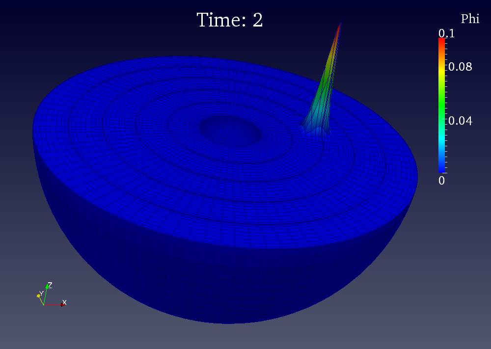
Figure 1: Topology of the numerical grid and the initial pulse perturbation on the equatorial plane. We only show 5 concentric shells of width 2 spanning the radial coordinate domain $\rho\in[1.99,12]$ with an expansion into spherical harmonics of order 47. The simulations presented in Sec. III use 40 such shells with a spherical harmonic expansion of order 87.

We employ hyperboloidal scri-fixing Zenginoglu (2008) to compute the unbounded domain solution and the signal at infinity as measured by idealized observers. The coordinates are constructed using the hyperboloidal layer method Zenginoglu (2011a) based on the ingoing Eddington–Finkelstein coordinates in the interior (Appendix A). Setting the Schwarzschild mass $M$, which provides the scale for the coordinates, to unity, the coordinate domain in the radial direction is $\rho\in[1.99,12]$ where $\rho=2$ corresponds to the event horizon and $\rho=12$ corresponds to null infinity. The interface to the hyperboloidal layer is at $\rho=8$. The hyperboloidal layer consists of the two outermost shells on the grid in Fig. 1.

The simulations presented in the results section (Sec. III) employ 40 concentric shells with 7 collocation points each and a spherical harmonic expansion of degree 87. For Fig. 1 we use a sparse grid for clarity of visualization. The Gaussian pulse (2) is based at $x^{\prime\mu}=\{t^{\prime},x^{\prime},y^{\prime},z^{\prime}\}=\{2,6,0,0\}$. Our results are robust under variation of parameter values.

We set the standard deviation as $\sigma=0.2$ unless otherwise stated, thus giving a 10:1 ratio of the radius of the event horizon to the scale of the source. We would obtain the Green function in the limit of vanishing width of the Gaussian and infinite numerical resolution. Our numerical approximation can be improved using smaller $\sigma$ and higher resolution.

III Results

III.1 Qualitative description

It is well-known that a generic scalar field in Schwarzschild spacetime dissipates to infinity in an exponentially decaying ringing and a polynomially decaying tail. The fast dissipation is confirmed in the top panel of Fig. 2, which shows the time evolution of the field as measured by an observer on the positive $z$ axis at null infinity. Following the initial pulse, we see more structure that becomes visible on a log scale in the bottom panel. There seems to be a recurring signal caused by the initial perturbation that disappears at late times when the polynomial decay dominates.

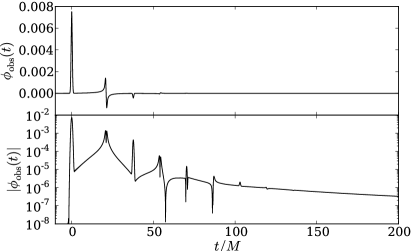
Figure 2: Top: The evolution of the scalar field generated by a compact source at $6M$ on the positive $x$ axis as measured by an observer at future null infinity on the positive $z$ axis. Bottom: The absolute value of the same field on a log scale, showing the detailed structure in the amplitude.

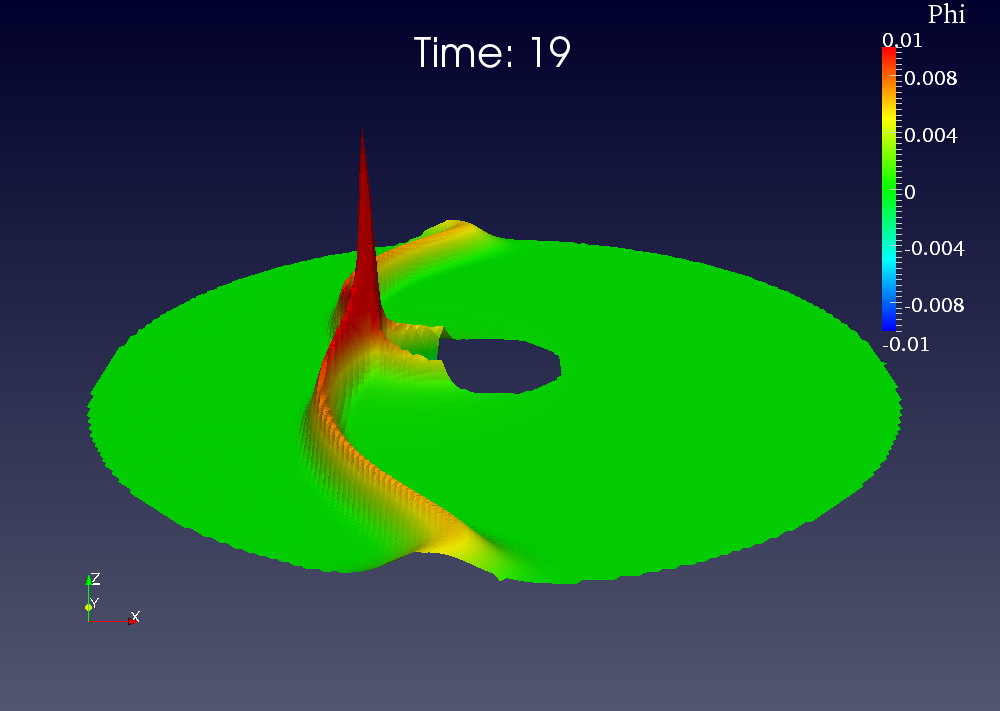
Figure 3: Formation of the first caustic echo from the initial pulse in Fig. 1. We plot a generic bird’s eye view onto the equatorial plane. A movie of the dynamical evolution, including a top to bottom view, can be seen online vid (a). The color and height of the surface is determined by the amplitude of the scalar field $\phi$. The wavefront of the direct signal has a Gaussian profile and forms a cardioid shape around the event horizon, which is typical of caustic formation. The amplitude amplification is clearly visible. The first caustic echo forms in the wake of the caustic and is seen as a wavefront in the vicinity of the horizon. It generates a second caustic echo plotted in Fig. 4.

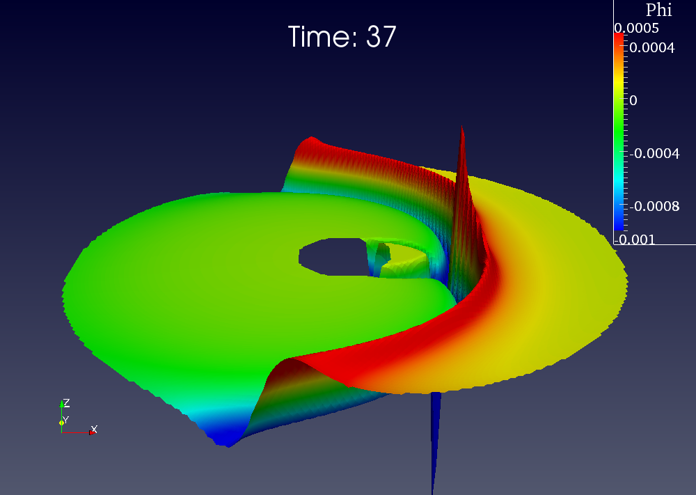
Figure 4: Formation of the second caustic echo. The profile of the signal from the wavefront of the first echo, seen at the boundary, is not a Gaussian but its Hilbert transformation (see Sec. III.3). The wavefront of the second caustic echo near the horizon is strictly negative and has a negative Gaussian profile (see boundary profile in Fig. 5).

The dynamics behind Fig. 2 can be seen more clearly in three-dimensional plots. In Figs. 3–6 we show snapshots from the evolution of $\phi$ on the equatorial plane. We set the width of the Gaussian source to $\sigma=0.3M$ for visualization.

The curvature of spacetime near the black hole causes the wavefront triggered by the initial pulse perturbation in Fig. 1 to bend and to focus forming a half-cardioid shape typical of caustic formation (Fig. 3). At the cusp of the cardioid, by the antipodal point to the initial perturbation near the black hole, the wavefront passes through itself thus forming a caustic. The caustic moves out to infinity along the negative $x$ axis and leaves an echo in its wake. This secondary wavefront again forms a cardioid shape with the cusp on the other side of the black hole (Fig. 4). This process repeats itself resulting in echoes that reach observers in regular time intervals (Figs. 5 and 6).

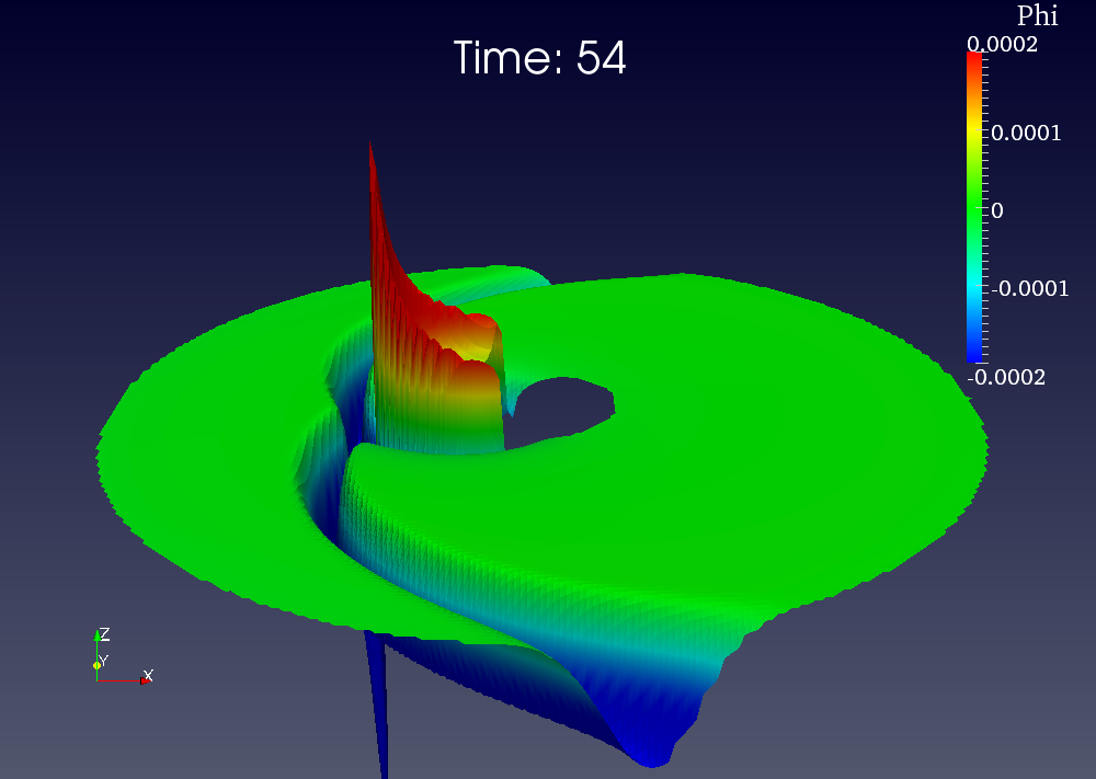
Figure 5: Formation of the third caustic echo. The second caustic echo has a negative Gaussian profile as seen at the boundary. The profile of the third echo is clearer in Fig. 6.

The figures suggest that the echoes are due to partial trapping of the initial energy at the photon sphere at areal coordinate $3M$. Part of the wavefront from the initial perturbation dissipates directly to infinity, part of it falls into the black hole, and part is trapped near the horizon forming so-called “surface waves” propagating on the photon sphere Ames and Thorne (1968); Goebel (1972); Andersson (1994); Decanini et al. (2010). The trapped signal goes through two caustics upon each full revolution and leaks out energy to infinity in the form of propagating wavefronts that we call caustic echoes.

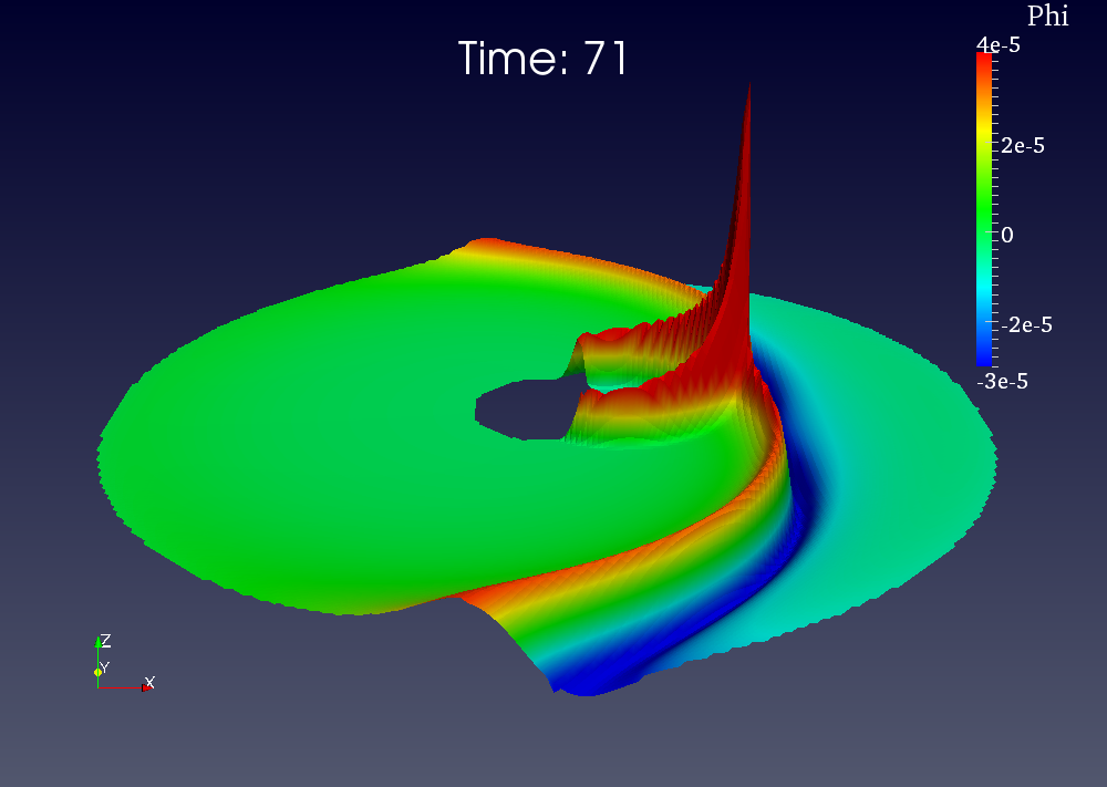
Figure 6: Formation of the fourth caustic echo. The profile of the third caustic echo is the Hilbert transform of the negative Gaussian, which is the negative of the profile of the first caustic echo seen in Fig. 4. The fourth caustic echo emanating from the horizon has a positive Gaussian profile like the direct signal, thus completing the fourfold cyle.

The profiles of the caustic echoes follow a certain pattern. The direct signal has the profile of a Gaussian in accordance with the source (Figs. 1 and 3). The shape of the first caustic echo (see the boundary profile in Fig. 4) is the Hilbert transform of the direct Gaussian signal, which we refer to as a Dawsonian, and is discussed in more detail in Sec. III.3. The second echo is a negative Gaussian (Fig. 5) and finally the fourth echo is a negative Dawsonian (Fig. 6). The wavefront emanating from the wake of the fourth echo has a Gaussian profile just like the initial signal, thereby completing the fourfold cycle (Fig. 6).

This is the demonstration of the fourfold structure first discovered in General Relativity by Ori Ori and analyzed by Casals et al. Casals et al. (2009, 2010). A visualization of the time evolution can be found on the internet vid (a). In the following, we present a detailed quantitative understanding of the data presented in Fig. 2. We present analysis for the measurements of an observer at future null infinity on the $z$ axis, unless stated otherwise.

III.2 Arrival and decay of caustic echoes

The first feature seen by the observer in Fig. 2 is a narrow Gaussian pulse that we refer to as the direct signal, which is the part of the perturbation that propagates directly to the observer. We set the observer’s clock to zero by the arrival time of the direct signal’s maximum. The arrival times of the subsequent caustic echoes are plotted in Fig. 7.

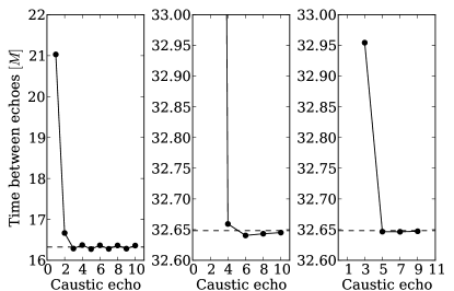
Figure 7: Time differences between caustic echoes indicating agreement with theoretical prediction based on null geodesic revolution times around the photon sphere at $3M$. Our measurement of the arrival times for differently shaped echoes leads to an artificial, systematic deviation from the theoretical prediction ($\pi\sqrt{27}M$, dashed line), which averages out (left panel). When similarly shaped echoes are compared, however, the measured time differences (between even echoes in the middle panel and between odd echoes in the right panel) agree accurately with the revolution time of null geodesics around the photon sphere given by $T_{{\rm full}}=2\pi\sqrt{27}M\approx 32.65M$.

Even and odd echoes, that is, echoes resulting from the wavefront passing through an even or odd number of caustics, have different profiles (see Figs. 2-6 and Sec. III.3). Therefore, it is appropriate to consider the arrival times of even and odd echoes separately. We extract the times between even echoes by fitting a Gaussian and reading off the time at which the peak amplitude arrives at the observer (middle panel of Fig. 7). We extract the times between odd echoes by fitting their time derivative to a Gaussian and finding the time at which the peak of the derivative is maximal (right panel of Fig. 7).

The arrival times of caustic echoes approach a constant value. This observation is explained through the generation mechanism behind the echoes, namely, the revolution of trapped energy at the photon sphere along null geodesics. The quantitative prediction of the arrival times requires only the study of high-frequency wave propagation for which it suffices to employ the geometrical optics approximation. An analysis of solutions to the scalar wave equation in Schwarzschild spacetime with localized energy has been performed by Stewart Stewart (1989). Stewart shows that the peak amplitude propagates along null geodesics, which orbit the photon sphere with a period of $T_{{\rm full}}=2\pi\sqrt{27}M\approx 32.6484M$. The half-period for the formation of each successive caustic is then $T_{{\rm half}}=\pi\sqrt{27}M\approx 16.3242M$. These values are plotted as dashed lines in Fig. 7 and indicate good agreement of the measured arrival times with the theoretical prediction. The best-fit value for the successive echoes shown in the left panel of Fig. 7 agrees with $T_{{\rm half}}$ to 4 significant digits.

The geometrical optics approximation is a short-wave (or high-frequency) approximation, and should therefore agree with the large $\ell$ limit of quasinormal modes. In this limit, the quasinormal mode frequencies can be expressed analytically as Ferrari and Mashhoon (1984); Iyer and Will (1987)

$$M\omega^{m=\ell}_{\ell n}\sim\frac{1}{\sqrt{27}}\big{(}\ell-i(n+1/2)\big{)}.$$ (4)

The real part of the frequency (divided by $\ell$) corresponds to the full orbital frequency $2\pi/T_{\rm full}$ of null rays on the unstable photon orbit. Thus, the time between successive even or odd caustic echoes is related to the real part of quasinormal mode frequencies in the large $\ell$ limit, which in turn are related to properties of null geodesics at or near the unstable photon orbit.

From (4) it is clear that the amplitude of caustic echoes should decay exponentially with a decay rate given by the imaginary part of the large $\ell$ frequency for the lowest overtone (hence longest decay time), $n=0$. The same decay rate can be calculated from the geometrical optics limit Stewart (1989) and is given by the Lyapunov exponent of unstable photon orbits Goebel (1972); Cardoso et al. (2009).

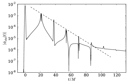
Figure 8: Amplitude decay of the field in Fig. 2. The dashed line shows the exponential decay implied by the imaginary part of the $n=0$ overtone of the quasinormal mode in the large $\ell$ limit (4), or equivalently the Lyapunov exponent $\lambda$ of the null geodesics near the unstable photon orbit.

Figure 2 indicates that the amplitude of each caustic echo decays exponentially with time until the backscatter off the background curvature dominates. Zooming into the interval before the tail-dominated domain, Fig. 8 shows visual agreement between the data and the theoretically predicted decay rate of $\lambda=1/(2\sqrt{27})M^{-1}\approx 0.096225M^{-1}$. For comparison, the decay rate associated with the peak amplitudes of the even (odd) caustic echoes obtained by fitting to $Ae^{-\lambda_{\rm num}t}$ gives $\lambda_{\rm num}=0.103M^{-1}$ ($0.097M^{-1}$).

The arrival and decay times of caustic echoes approach their predicted values from the geometrical optics approximation (or equivalently the large $\ell$ quasinormal mode limit) very fast. The first few echoes following the direct signal, however, deviate from these limiting values considerably (Fig. 7). This deviation is due to the propagation of the first caustic echo along a null geodesic that is farther away from the photon sphere than the subsequent echoes.

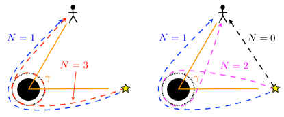
Figure 9: Cartoon depicting several null geodesics connecting the source (yellow star) to the observer (stick figure) for a generic relative angle, $\gamma\in[0,\pi)$. The black hole is represented by a solid black disk and its unstable photon orbit by a dotted circle. Left: The null geodesic paths corresponding to the first two odd caustic echoes. Right: The null geodesic paths corresponding to the first three signals.

A schematic diagram of the propagation of the first three signals is given in Fig. 9. We label the echoes by the order in time in which they appear, or equivalently by the number of caustics $N$ that the wavefront has passed through before leaving the photon sphere. Consider the the first pulse after the direct signal that reaches the observer, the $N=1$ echo. The pulse travels along the null geodesic connecting the source to the observer wrapping partially around the far side of the black hole. The angle swept through by this null geodesic is $\Delta\varphi_{1}=3\pi/2$. The null geodesic corresponding to the $N=3$ echo makes a full orbit around the black hole so that the angle swept through is $\Delta\varphi_{3}=7\pi/2$. For any relative angle between the source and observer, $\gamma\in[0,\pi]$, it is clear from Fig. 9 that the time between successive even or odd caustic echoes approaches the period for a null geodesic to make a full orbit around the photon sphere; this is a universal property of the black hole independent of the source-observer configuration.

For generic source-observer configurations, the time between caustic echoes depends on the angle $\gamma$ between the source and observer. The times between successive caustic echoes are given by

$$\Delta T_{N}(\gamma)=\left\{\begin{array}[]{lcc}\displaystyle\frac{\gamma}{\pi}\,T_{\rm full}&,&N{\rm~{}even}\\ &&\\ \displaystyle\frac{\pi-\gamma}{\pi}\,T_{\rm full}&,&N{\rm~{}odd}\end{array}\right.$$ (8)

The cases $\gamma=0,\pi$ are degenerate because $\Delta T_{N}=0$ for either an even or odd echo. These observers see a twofold cycle as opposed to a fourfold cycle, and the peak amplitude of the signal is amplified as seen in Figs. 3–6. The amplification cannot be treated in the geometrical optics approximation because the amplitude at caustic points is unbounded in this limit. We discuss the twofold cycle and the energy amplification for degenerate observers in Sec. III.4.

III.3 Profiles of caustic echoes

The profiles of caustic echoes transform by propagating through caustics, which leads to a fourfold cycle Ori ; Casals et al. (2009, 2010). In this section, we analyze in detail the structure of the pulse profiles.

Figure 10 shows the profiles for the same source-observer configuration as in the previous section. The first pulse in the upper left panel is the direct signal and the subsequent pulses are the caustic echoes. The fourfold cycle presented in each row repeats itself until the signal is dominated by the tail (third row of Fig. 10). More caustic echoes are visible in the local decay rate (Fig. 15).

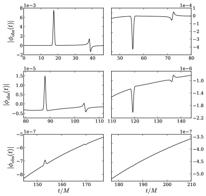
Figure 10: The first 12 pulses (direct signal plus 11 caustic echoes) seen by an observer on the positive $z$ axis at future null infinity. The profiles of the caustic echoes are repeated in a fourfold cycle as is clearly seen in the first two rows. In the last row, the tail effect from backscattering dominates the signal.

Using the geometrical optics approximation in Appendix C, we show that passing through a caustic induces a phase shift of the wavefront in the frequency domain by $-\pi/2$ radians and is equivalent to a Hilbert transform (47). The phase change of light traveling through a caustic is a well-known effect in optics, called the Gouy phase shift, and was discovered in 1890 Gouy (1890) (for a more recent discussion see Chapter 9.5 of Hartmann (2009)). The fourfold structure of the Green function is then a simple consequence of trapped null geodesics passing through caustics with each passage causing a phase shift by $-\pi/2$, completing a full cycle of $2\pi$ in four echoes.

The Green function in the geometrical optics approximation is given by (50)

$$G(x,x^{\prime})\sim{} \sum_{N=0}^{\infty}\big{|}A_{0}({\bf x},{\bf x}^{\prime})\big{|}\,\theta(t-t^{\prime}-T_{N-1}({\bf x},{\bf x}^{\prime}))$$

$${\hskip 18.06749pt}\times{\rm Re}\big{\{}H_{N}\big{[}\delta(t-t^{\prime}-T_{N}({\bf x},{\bf x}^{\prime}))\big{]}\big{\}}.$$ (9)

Here, $T_{N}({\bf x},{\bf x}^{\prime})$ is the coordinate time along a null geodesic connecting the spatial points ${\bf x}$ and ${\bf x}^{\prime}$ and passing through $N$ caustics, $H_{N}$ denotes $N$ applications of the Hilbert transform (thus phase shifting its argument by $-N\pi/2$), the step function ensures causality (with $T_{-1}({\bf x},{\bf x}^{\prime})\equiv 0$), and $A_{0}({\bf x},{\bf x}^{\prime})$ is the leading order field amplitude in the geometrical optics limit (see Appendix C for the derivation). The field is obtained by the convolution of the Green function with the source $S(x)$

$$\phi(x) =\int_{x^{\prime}}G(x,x^{\prime})S(x^{\prime})\sim\sum_{N=0}^{\infty}\phi_{N}(x),$$ (10)

where $\int_{x^{\prime}}\equiv\int d^{4}x^{\prime}\sqrt{-g(x^{\prime})}$ with $g$ the determinant of the spacetime metric, and $\phi_{N}(x)$ is the field evaluated in the geometrical optics approximation associated with the passage of the wavefront through $N$ caustics.

Equation (10) gives us a quantitative prescription for the profiles of the wavefronts after propagation through $N$ caustics. For $N=0$, the Hilbert transform $H_{0}$ returns its argument. Hence the direct signal obtained from the convolution of the approximate Green function (9) with the Gaussian source (2) is proportional to a Gaussian as confirmed in the upper left panel of Fig. 10. For $N=1$ the Hilbert transform $H_{1}$ applies a phase shift by $-\pi/2$ radians to the signal entering the caustic. For the delta distribution in (9) this is given by (46). Interestingly, (46) has a different singularity structure than the delta distribution and has support in the interior of the forward light cone of ${\bf x}^{\prime}$. Hence, this contribution adds to any tail piece from backscattering once the wavefront has passed through an odd caustic. The caustic thus smears out the (sharp) delta distribution that gets refocused to a delta distribution when passing through the next caustic.

For the first caustic echo we get from (10)

$$\phi_{1}(x)={} \frac{1}{(2\pi\sigma^{2})^{2}}\int_{{\bf x}^{\prime}}|A_{0}({\bf x},{\bf x}^{\prime})|\exp\left(-\frac{({\bf x}^{\prime}-{\bf x}_{0})^{2}}{2\sigma^{2}}\right)$$

$$\times {\rm Re}\bigg{[}\int_{-\infty}^{\infty}\frac{d\omega}{2\pi}\,\exp\left(-\frac{i\pi}{2}-i\omega\big{(}t-T_{1}({\bf x},{\bf x}^{\prime})\big{)}\right)$$

$${\hskip 28.90755pt}\times\int_{-\infty}^{t-T_{1}({\bf x},{\bf x}^{\prime})}{\hskip-10.84006pt}dt^{\prime}\exp\!\left(i\omega t^{\prime}-\frac{(t^{\prime}-t_{0})^{2}}{2\sigma^{2}}\right)\!\!\bigg{]}.$$ (11)

Integrating over $t^{\prime}$ (assuming $t-T_{1}({\bf x},{\bf x}^{\prime})\gtrsim t_{0}+\sigma$ so that the upper integration limit is replaced by $\infty$) and $\omega$, and assuming that the spatial part of the Gaussian is sufficiently narrow to be replaced by a delta distribution yields

$$\phi_{1}(x)\approx-|A_{0}({\bf x},{\bf x}_{0})|D\big{(}t-t_{0}-T_{1}({\bf x},{\bf x}_{0}),\sigma\big{)},$$ (12)

where

$$D(y,\sigma)\equiv e^{-y^{2}/(2\sigma^{2})}{\rm erfi}\left(-\frac{y}{\sqrt{2}\,\sigma}\right)$$ (13)

is related to Dawson’s integral Duoandikoetxea (2008). We will refer to (13) as the “Dawsonian” below.

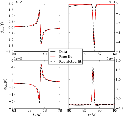
Figure 11: The first four caustic echoes in the numerical solution (black) along with two fits to a Dawsonian using the geometrical optics approximation (red and dashed black). The numerical solution is fit to Eq. (12) with the amplitude, time of arrival, and width as fitting parameters. The fit is so well that the red and the black lines are hardly distinguishable. The black dashed line is a restricted fit where only the amplitude is fitted for and the time of arrival and the width are set by the numerical solution and the Gaussian source width, respectively. The quality of the fits indicate that the geometrical optics approximation captures the profiles of the caustic echoes accurately via the Hilbert transform.

The upper left panel of Fig. 11 shows the first caustic echo (e.g., the second pulse in the upper left panel of Fig. 10) together with two different fits to a Dawsonian using (12). The black line is the numerical data and the red line is a fit to $aD(t-b,c)+d$ with $a=-2.8\times 10^{-3}$, $b=38.64M$, $c=0.28M$, and $d=2.4\times 10^{-5}$. Note that the best-fit value for $c=0.28M$ differs substantially from the original width of the Gaussian source of $\sigma=0.2M$. This free fit is remarkably good over a large interval around $T_{1}({\bf x},{\bf x}_{0})=b$.

The black dashed line in Fig. 11 shows the approximation (12) with $\sigma=0.2M$ (i.e., the width of the Gaussian source) and $T_{1}({\bf x},{\bf x}_{0})$ fixed to the value extracted from the numerical simulation; only the amplitude is fitted for. Despite the crudity of the approximations, the restricted fit captures qualitative features of the $N=1$ echo rather well. The agreement indicates that the Green function in the geometrical optics approximation is suitable to describe the propagation of wavefronts through caustics in terms of Hilbert transformations. The remaining panels in Fig. 11 for the next three caustic echoes show similar results.

Our discussion so far covers wavefront propagation through caustics for relatively narrow pulses providing an approximation to the Green function. We confirmed the action of a Hilbert transform at caustics using other waveforms as well.

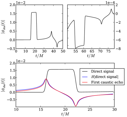
Figure 12: Top: The caustic echoes of a square pulse source lasting for $6M$ and located at $6M$ on the positive $x$ axis as seen by an observer on the positive $z$ axis at future null infinity. Bottom: The direct signal of the square pulse (black), its Hilbert transform (blue), and the first caustic echo appropriately shifted and rescaled to match the amplitude of the blue curve. Despite the long time scale of the square pulse, its corresponding wavefronts are still Hilbert transformed through caustics.

The top panels in Fig. 12 show a fourfold cycle triggered by an initial square profile, that is, a pulse localized in space but persisting for a longer time scale than the time scale of the black hole. In the lower panel of Fig. 12 we plot the direct signal (black curve) and compare its Hilbert transform (blue curve) to the rescaled and shifted profile of the $N=1$ caustic echo from the numerical simulation (red curve). The agreement between the blue and the red curves implies that the wavefronts are indeed Hilbert transformed through caustics.

III.4 The twofold cycle and the caustic line

Equation (8) indicates that for angles $\gamma=0,\pi$ between the source and the observer, the structure of the measured signal is degenerate. This is the caustic line where caustic echoes merge (the $x$ axis in our simulations). Even and odd echoes arrive at the same time at the caustic line, therefore we obtain a twofold cycle as opposed to a fourfold one. Hence, the number of echoes in a cycle is observer-dependent but the existence of a cyclic feature is universal and associated with the trapping of energy near the black hole.

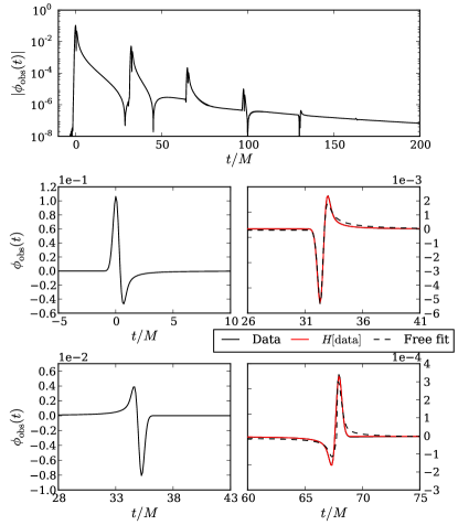
Figure 13: Top: The evolution of the scalar field as measured by an observer at future null infinity on the negative $x$ axis. Middle: Degenerate echoes as measured by the same observer. Because the source is also on the $x$ axis, the observer only sees a twofold cycle. Also shown is the Hilbert transform of the signal (red) in the left panel (rescaled and shifted to compare with the caustic echo) and the free fit to the geometrical optics approximation (dashed). Bottom: Same as above except that the observer is on the positive $x$ axis. Note the differences in the caustic echo profiles.

Consider the top panel of Fig. 13. The first pulse is formed by the direct signal and the $N=1$ caustic echo. The next pulse arrives after a full revolution time $T_{\rm full}$ and consists of the $N=2,3$ caustic echoes. (Compare Fig. 9 or Figs. 3-6 with an observer along the caustic line to visualize the simultaneous arrival of echoes.)

The echoes on the caustic line also undergo a Hilbert transformation. The middle panel of Fig. 13 shows the first ($N=0,1$) and the second ($N=2,3$) degenerate echoes for an observer on the negative $x$ axis ($\gamma=\pi$), while the bottom panel of Fig. 13 shows the first ($N=1,2$) and the second ($N=3,4$) degenerate echoes for an observer on the positive $x$ axis ($\gamma=0$). The $N=0,1$ degeneracy for the $\gamma=\pi$ observer leads with a Gaussian profile which is Hilbert transformed at its peak to a Dawsonian for the trailing half of the signal. The $N=1,2$ degeneracy for the $\gamma=0$ observer leads with a Dawsonian profile which is Hilbert transformed at its zero crossing to a Gaussian for the trailing half of the signal. The next degenerate echoes are the Hilbert transforms of the previous ones as indicated in the middle and bottom right panels of Fig. 13. The red curves are the Hilbert transforms of the previous degenerate echoes to the left, suitably shifted in time and rescaled in amplitude for comparison.

The amplitude of the wave becomes singular along the caustic line in the geometrical optics approximation. However, given that the echoes can be characterized via Hilbert transforms whenever the wavefront passes through a caustic, the time dependence of the signal may be captured by the geometrical optics approximation. To test this, we fit the data to the profile implied by the convolution of the Green function in the geometrical optics approximation (9) with the source (2). More specifically, the $N=0,1$ degeneracy for the $\gamma=\pi$ observer is fit to

$$a\,e^{-(t-b)^{2}/(2d^{2})}+c\,\theta(t-b)D(t-b,d)$$ (14)

where $b$ is approximately the time of arrival $T_{0}=T_{1}$, while for the $N=1,2$ degeneracy for the $\gamma=0$ observer the fit is

$$a\,D(t-b,d)+c\,\theta(t-b)\,e^{-(t-b)^{2}/(2d^{2})}$$ (15)

with $b$ approximately $T_{1}=T_{2}$. In both cases, the amplitudes ($a,c$), the time of arrival ($b$), and the width are arbitrary ($d$). The results of this free fit are shown in the middle and bottom right panels of Fig. 13 (dashed lines). Despite its breakdown, the geometrical optics approximation captures the basic time-dependence of the profiles fairly well.

The wavefront is focused and its amplitude is magnified along the caustic line (see Figs. 3-6). We next characterize this magnification at the caustic relative to the echoes it generates in relation to the scale of the wavefront. The computations of such relations go beyond the geometrical optics approximation and require elements of geometric diffraction theory. In Kay and Keller (1954) Kay and Keller show that the peak amplitude at a caustic with a perfect focus increases as $\sigma^{-1/2}$, where $\sigma$ provides the scale for the width of the wavefront.

Note that the caustic and its echoes have different shapes. Therefore, a comparison of their peak amplitude might be misleading. Instead, we compare the energy radiated to an observer at infinity during a certain time interval $I$,

$$E=\frac{1}{2}\int_{I}dt\,\big{|}\dot{\phi}(t)\big{|}^{2}.$$ (16)

To make sure that the amplification factor is not influenced by the shape of the echoes, we compute it with respect to both Dawsonian and Gaussian shapes. The compared signals are plotted in the top panel of Fig. 14. We label the measurement of the caustic ($N=1,2$) by an observer at $\gamma=0$ as $A$. An observer at $\gamma=\pi/2$ measures not the caustic but its echoes. The Dawsonian echo ($N=1$) is labeled as $B$, the Gaussian one ($N=2$) as $C$.

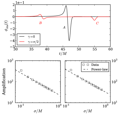
Figure 14: Top: A caustic ($A$) at $\gamma=0$ (black), the $N=1$ echo ($B$), and the $N=2$ ($C$) echo along $\gamma=\pi/2$ (red). Bottom: The amplification of the energy of $A$ relative to $B$ (left) and $C$ (right) along with an inverse power law fit (dashed).

We compute the energy integral over a sufficiently large time interval centered at the pulse so that the energy difference to a larger interval is negligible (less than $1\%$). The amplification is then computed via

$${\rm Amplification}\equiv\frac{E_{A}}{E_{B,C}}.$$ (17)

We plot the amplification on a log-log scale as a function of Gaussian widths $\sigma$ in the bottom two panels of Fig. 14. The amplification factor can be fit accurately by an inverse power law of the form $a\sigma^{p}$ where $(a_{B},p_{B})=(23.7,-1.03)$ (bottom left) and $(a_{C},p_{C})=(26.1,-1.02)$ (bottom right). Hence, the data suggests that the energy amplification at the caustic goes as $\sigma^{-1}$ as the width of the Gaussian source becomes more narrow. This seems in accordance with the calculation of Kay and Keller for caustics with a perfect focus Kay and Keller (1954).

We emphasize, however, that we cover only a small range of scales ($\sigma\in[0.1,0.6]$) and that we did not mathematically derive the scale dependence of the energy at caustics formed by a Schwarzschild black hole. Including smaller values for $\sigma$ will most likely follow an inverse power law but may change the value in the fit. Therefore, our numerical result should be interpreted carefully.

There are extensive studies on the detailed behavior of solutions to wave equations near caustics, including not only their energy magnification but also their shapes in different directions away from the caustic line. Such an analysis is outside the scope of this paper but provides an interesting subject for future research.

III.5 Propagation within the light cone

We have shown that essential properties of the Green function can already be understood in the geometrical optics limit. We also discussed effects due to the finite wavelength of the wave, which plays a role in the energy magnification at caustics. In this section, we consider features at the largest scale, the spacetime curvature.

It is well-known that the Green function propagates also inside the null cone in curved spacetimes due to the backscatter of the field off the background curvature. The field within the null cone decays polynomially following the so-called Price power law Price (1972). The rate of the decay for idealized observers at null infinity is different than the rate at finite distances Gundlach et al. (1994). While the null infinity rate is the relevant one with respect to idealized observers, the finite distance rate is the one that effects the self-force on a particle. Both rates are plotted in Fig. 15.

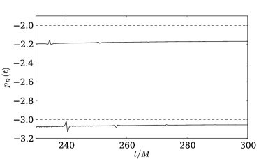
Figure 15: Polynomial decay rates asymptotically approaching $p=-2$ for an idealized observer at null infinity (top solid curve), and $p=-3$ for a finite distance observer at $r=4M$ (bottom solid curve). The theoretical asymptotic decay rates are plotted as dashed lines. Caustic echoes are still visible in the local power plot at late times.

The theoretical decay rates are valid asymptotically in time. One can obtain a good estimate of the rates by computing a local in time rate along the worldline of an observer at $r=R$ defined by

$$p_{R}(t)=\frac{d\ln|\phi(t,R)|}{d\ln t}.$$ (18)

The theoretical asymptotic decay rate for a generic scalar perturbation in Schwarzschild spacetime is for idealized observers at null infinity $p_{\infty}=-2$ and for finite distance observers $p_{R}=-3$. Figure 15 confirms the approach of the local power to the asymptotic rate. The theoretical predictions are plotted as dashed lines.

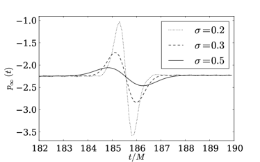
Figure 16: The visibility of a caustic echo in the local power at null infinity for three different values of the width of the initial Gaussian source (2). More caustic echoes are visible at late times for narrower Gaussians.

In discussions of gravitational lensing it is often stated that, under certain assumptions and with ideal instruments, one would see infinitely many images of a source with an eternal worldline Perlick (2010). Considering the geometrical optics limit, one might be inclined to think that for arbitrarily narrow Gaussians we would observe arbitrarily many caustic echoes. We show in Fig. 16 a caustic echo visible in the local power of the signal at null infinity for three different values of $\sigma$ for the Gaussian source (2). The caustic echo is more pronounced for smaller values of $\sigma$ indicating that the narrower our source, the more caustic echoes we see in the late time signal.

However, it is also clear that for any positive value of $\sigma$ we can only see a finite number of caustic echoes because the amplitude of each echo decays exponentially in time whereas the backscatter off curvature decays only polynomially. This observation implies that, even with ideal instruments, we can measure only a finite number of “images” for any given source because eventually the polynomial decay will win over the exponentially weakening echo. Proofs of infinitely many images of sources typically consider the geodesic structure of spacetimes and neglect backscatter Hasse and Perlick (2002).

III.6 Putting the pieces together

We presented in previous sections a quantitative understanding of each feature in the evolution of a scalar perturbation triggered by a narrow Gaussian wave package. Dissecting the signal observed at infinity (Fig. 2) we explained the arrival times, the exponential decay, the shapes of the echoes, and the late time behavior of the scalar field. In this section, we bring these elements together into a heuristic formula that captures the essential features of the evolution remarkably well.

The shape, the arrival times, and the exponential decay of caustic echoes can be accurately described in the geometrical optics limit as discussed in Secs. III.2 and III.3. We derived an analytic expression for the Schwarzschild Green function in this limit (Appendix B), presented for the first time in this paper as far as we are aware. Using this analytic knowledge we approximate the signal by

$$\phi_{\rm geom} =A_{0}\bigg{[}e^{-(t-T_{0})^{2}/(2\sigma_{a}^{2})}+e^{-\lambda(t-T_{0})}$$

$$\times{\rm Re}\sum_{n=1}^{N}\theta(t-T_{n-1}-\delta T)\,e^{-in\pi/2}$$

$$\times\bigg{(}e^{-(t-T_{n}-\delta T)^{2}/(2\sigma_{a}^{2})}-iD(t-T_{n}-\delta T,\sigma_{a})\bigg{)}\bigg{]}.$$ (19)

where $\lambda\approx 0.096225$ is the Lyapunov exponent for unstable photon orbits, $T_{0}$ is the time of arrival of the direct signal to the observer, and $T_{n}$ is the time of arrival for the $n^{\rm th}$ caustic echo (with $T_{-1}\equiv 0$). The latter is computed from $T_{n-1}+\delta T+\Delta T_{n}(\gamma)$ using (8). The quantity $\delta T$ accounts for the fact that the time between successive caustic echoes is not immediately given by $\Delta T_{n}(\gamma)$ (Fig. 7). We found it sufficient to approximate $\delta T$ by $T_{2}-T_{0}-T_{\rm full}$, which is independent of $\gamma$. Only $T_{0}$ and $\delta T$ (or $T_{2}$) are extracted from the numerical simulation. We set $A_{0}=0.016$, $\sigma_{a}=0.28$, and the number of caustic echoes as $N=15$ specifically for the observer of Fig. 2.

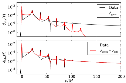
Figure 17: Reconstructing the numerical solution (black) using heuristic formulae (red). The top panel shows the structure of the field from the geometrical optics limit. The bottom panel includes the power law tail contribution. Despite the simple nature of the approximations, the field’s rich dynamics are captured remarkably well.

The geometrical optics formula for the scalar field agrees with the numerical data in the early part of the signal (top panel of Fig. 17). To match the late time behavior of the field we use the polynomial decay discussed in Sec. III.5. We include the tail only after the direct signal has reached the observer and set

$$\phi_{\rm tail}=Ct^{p}\,\theta(t-T_{0}),$$ (20)

with $C=-0.06$ and $p=-2.25$. Note that the asymptotic decay rate would be $p=-2$. The difference is due to the high order correction terms which are neglected in the above formula. One can include such correction terms by constructing more general fitting functions (see for example Bizon and Rostworowski (2010)). Recently, Casals and Ottewill computed the first three orders in the power law for the Schwarzschild Green function Casals and Ottewill (2012), which can also be used to improve the description of the tail. We found the simple expression above sufficiently accurate for our purposes. Better expressions for the tail fit might be needed for comparisons with more accurate approximations to the Green function, or for self-force computations.

Our heuristic formula for the full field is the sum of the geometrical optics contribution (19) and the tail contribution (20). Considering the simplicity of the assumptions that go into our heuristic expression, its agreement with numerical data is remarkable (bottom panel of Fig. 17).

Note that the addition of the tail not only improves the agreement with the data at late times but also captures the zero crossings between the caustic echoes at $t/M\approx 57$ and $86$. In typical numerical studies of the tail, the polynomially decaying part of the signal plays a role only at late times. Here, we see that it improves the fit between the echoes at relatively early times. This is because backscattering contributes even right after the direct signal has passed the observer. This feature is well-known and is captured in Hadamard’s ansatz for the Green function whenever $x$ and $x^{\prime}$ are connected by a unique geodesic Hadamard (1923); Poisson et al. (2011).

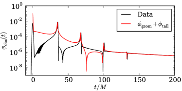
Figure 18: Reconstructing the numerical solution (black) as seen by an observer at null infinity on the positive $x$ axis along the caustic line. The analytical approximation (red) disagrees significantly with the data between the caustic echoes at early times.

Our heuristic formula should fail along the caustic line (the $x$ axis in our simulations) because the geometrical optics approximation breaks down at caustics. We find that (19) and (20) on the caustic line works well for the high-frequency part of the signal (i.e., the caustic echoes themselves) and for describing the late-time tail (Fig. 18), but cannot capture the effects of early-time backscattering (compare to Fig. 17 for the observer at $\gamma=\pi/2$). Also, the formula has zero crossings which do not occur at the correct times. Near a caustic the wavefronts are focused and magnified thus distorting the shape of the wavepacket (see Figs. 3-6). Hence, the echoes have a comparatively larger amplitude than the direct signal (Fig. 18). These features are not accounted for in the geometrical optics limit and require a more complete description of wave optics in curved spacetime.

Further analysis is needed to improve on our heuristic formula. For example, one can include corrections to the geometrical optics approximation using the expansions presented in Dolan and Ottewill (2009) or combine other quasilocal expansions of the Green function Ottewill and Wardell (2011) and its Padé resummation Casals et al. (2009). These potential directions for research are left for future work.

IV Conclusions

We numerically solved the scalar wave equation on a Schwarzschild background (1) with a narrow Gaussian source (2) thus yielding an approximation to the Schwarzschild Green function (3). For the numerical computations we used the Spectral Einstein Code SpEC SpE .

The main result of our study is the numerical approximation of the full retarded Schwarzschild Green function in the time domain. This computation allowed us to demonstrate a cyclic singularity structure due to the trapping of energy near the photon sphere.

The numerical evolution, visualized in Figs. 3-6 and in vid (a), proceeds as follows. The narrow Gaussian source triggers a high-frequency wavefront that propagates along null geodesics in accordance with geometrical optics. Part of the energy of the initial wavefront gets trapped at the black hole horizon and leaks out to infinity decaying exponentially in time. At each half revolution around the photon sphere the trapped wavefront forms a caustic resulting in echoes that propagate out to infinity. The wavefront undergoes a Hilbert transform at the caustics causing a $-\pi/2$ phase shift in its profile, which results in a fourfold cycle of caustic echoes seen by generic observers. This cycle is known as the fourfold singularity structure of the retarded Green function Ori ; Casals et al. (2009, 2010); Dolan and Ottewill (2011); Casals and Nolan (2012); Harte and Drivas (2012).

The fourfold structure is a recent discovery in the context of curved spacetimes but, in hindsight, it is a simple consequence of well-known facts. The $\pi/2$ phase shift of wavefronts at caustics has already been discovered in the late 19th century and is widely known as the Gouy phase shift in optics Gouy (1890); Hartmann (2009). Combined with the notion of trapping (e.g., due to the presence of a photon sphere), this knowledge immediately implies a fourfold cycle in a spherically symmetric, asymptotically flat spacetime . The viewpoint of a phase shift of the Green function at caustics seems more fundamental than the fourfold structure. For example, a phase shift may be observed in regions of moderate curvature due to gravitational lensing where no trapping occurs, whereas trapping is required for the observation of $n$-fold cycles. In addition, a nongeneric set of observers, those on the caustic line, see a twofold cycle. Hence, the number of echoes in a cycle is observer-dependent.

With the full numerical approximation to the Green function at hand, we also obtained an interesting result regarding gravitational lensing. If backscatter off background curvature is included, only a finite number of images are visible, even with ideal instruments, for any source of finite wavelength because caustic echoes decay exponentially in amplitude while backscatter (typically neglected in lensing studies) decays only polynomially.

Further results can be summarized as follows. The arrival and decay of successive caustic echoes are consistent with the orbital period and Lyapunov exponent of null geodesics trapped at the photon sphere. The arrival times of successive half-period echoes depend on the source-observer configuration, with degeneracy resulting in a twofold cycle when the source and the observer are aligned with the black hole. This is the caustic line along which the amplified signal propagates. The energy magnification at the caustic follows an inverse power law with the scale of the wavefront in accordance with predictions going beyond the geometrical optics limit Kay and Keller (1954). The backscatter follows well-known polynomial decay rates at null infinity and at finite distances, which limits the number of echoes measurable by observers.

We formulated an analytic approximation to the Schwarzschild Green function in the geometrical optics limit including wavefront propagation through caustics. Combined with our quantitative understanding of the dynamics, this formula allowed us to capture the essential features of the observed signal in a heuristic expression. Given the simplicity of our approximations, it is remarkable that the expression agrees so well with the numerical calculation.

The only sources of error in the numerical computation of the Schwarzschild Green function are the finite width of the Gaussian source (2) and the truncation error due to discretization of the scalar wave equation. The boundary error typically present in such simulations is eliminated by hyperboloidal scri-fixing in a layer Zenginoglu (2008, 2011a). We emphasize that hyperboloidal compactification is not necessary for the numerical study of the Green function near the black hole. Many of our results are reproducible using standard foliations. However, hyperboloidal compactification helps focusing the resolution to the strong field domain without contamination from artificial boundaries and without wasting computational resources on the asymptotic domain. It allows us to compute the long-time evolution accurately at low cost, and provides us direct numerical access to measurements of an idealized observer at future null infinity.

The error scales in our computation are related. To evolve a narrow Gaussian source, we need a large number of collocation points for the spectral expansion of the variables. Failure to do so results in Gibbs phenomena and contaminates the evolution. (Some high frequency noise in the late-time evolution can be seen in the lower curve of Fig. 15). Numerical convergence tests and the agreement between theory and experiment indicate that our errors are small but we did not present a detailed error analysis in this paper. Such an analysis will be required when comparing the numerical simulations to accurate approximations of the Green function or when computing the self-force acting on a particle using the numerically computed Green function. For these calculations, horizon-source ratios larger than 10:1 might be necessary. The numerical method must be further improved for very high ratios, possibly using a second order in space formulation Taylor et al. (2010), implicit-explicit time stepping Lau et al. (2009), and adaptive mesh refinement. There are also adapted methods to solve for high-frequency wave propagation, such as the frozen Gaussian beam method Lu and Yang (2011) or the butterfly algorithm Candes et al. (2009), that may improve the efficiency of the numerical simulation considerably.

An immediate extension of our study would be the numerical computation of retarded Green functions in Kerr spacetime. In rotating black hole spacetimes, frame dragging plays a role in the wavefront propagation. There is no photon sphere in Kerr spacetime; instead, there are spherical photon orbits bounded by the location of pro- and retrograde circular photon orbits Teo (2003) which may participate in the Cauchy evolution in a similar way as does the photon sphere in Schwarzschild spacetime. The large $\ell$ limit of the quasinormal mode spectrum and its relation to spherical photon orbits in Kerr spacetime have recently been analyzed in Yang et al. (2012). Such analytic knowledge can be combined with numerical experiments to reveal the structure of the Green function in Kerr spacetimes and to provide good approximations to it. The visualization of a numerical Kerr Green function simulation using SpEC can be found in vid (b).

An interesting application of numerical approximations of Green functions would be the computation of the self-force on a small compact object moving in a supermassive black hole spacetime. Note that the Green function provides a very general way of solving for wave propagation in a background spacetime. If good approximations to it can be found, possibly augmented by data from numerical computations, the method can be applied to essentially any problem on the given background via suitable convolutions. To this end, it may be useful to have sparse representations of the numerical Green function.

The improvement of Green function approximations may benefit from developments in various fields. Formation of caustics in black hole spacetimes is an example of the emergence of discrete structures from continuous ones, a hallmark of catastrophe theory Arnold (1984). A development of geometric diffraction theory and wave optics for black holes may allow us to compute the Green function through caustics without matching arguments while also providing more accurate analytical approximations. Exciting developments in these directions can be expected in the near future.

Appendix A Hyperboloidal layer with excision

In our numerical simulations we use hyperboloidal scri-fixing Zenginoglu (2008) in a layer Zenginoglu (2011a) attached to a finite Schwarzschild domain in ingoing Eddington–Finkelstein (iEF) coordinates. In this Appendix we describe the construction of such coordinates.

The Schwarzschild metric in standard Schwarzschild coordinates $\{t_{S},r,\vartheta,\varphi\}$ reads

$$g=-\left(1-\frac{2M}{r}\right)\,dt_{S}^{2}+\left(1-\frac{2M}{r}\right)^{-1}dr^{2}+r^{2}d\sigma^{2},$$

where $d\sigma^{2}=d\vartheta^{2}+\sin\vartheta^{2}d\varphi^{2}$ is the standard metric on the unit sphere. Ingoing Eddington–Finkelstein coordinates are constructed from Schwarzschild coordinates by the time transformation $t=t_{S}+2M\ln(r-2M)$, which leads to the metric

$$g = -\left(1-\frac{2M}{r}\right)\,dt^{2}+\frac{4M}{r}\,dt\,dr$$ (21)

$$+\left(1+\frac{2M}{r}\right)\,dr^{2}+r^{2}\,d\sigma^{2}.$$

The metric is regular at the horizon, $r=2M$, because the slices of the iEF foliation penetrate the future horizon without intersecting each other, as opposed to the slices of the standard Schwarzschild foliation which intersect at the bifurcation sphere. In a similar construction, iEF slices that intersect at spatial infinity can be transformed to hyperboloidal slices that foliate null infinity Zenginoglu (2011b). The hyperboloidal layer method that leads to such a slicing consists in the introduction of a compactifying coordinate in combination with a suitable time transformation. The compactifying coordinate $\rho$ can be defined via

$$r=\frac{\rho}{\Omega},\qquad\rm{where}\qquad\Omega=1-\left(\frac{\rho-\it{I}}{\it{S}-\it{I}}\right)^{4}\Theta(\rho-\it{I})\,.$$ (22)

Here, $\Theta$ is the Heaviside step function. The compactifying layer is attached at the interface $\rho=I$ and has a thickness of $S-I$ in local coordinates. The zero set of $\Omega$, namely $\rho=S$, corresponds to infinity. To avoid loss of resolution near infinity, we combine this spatial compactification with a time transformation. The time transformation is constructed requiring invariance of outgoing characteristic speeds Zenginoglu (2011a); Jasiulek (2012), or equivalently, of the outgoing null surfaces in local coordinates Bernuzzi et al. (2011); Zenginoglu and Khanna (2011). Outgoing null surfaces satisfy $u=t-\left(r+4M\log(r-2M)\right).$ The invariance condition translates to

$$t-\left(r+4M\log(r-2M)\right)=\tau-\left(\rho+4M\log(\rho-2M)\right).$$

This relation defines the hyperboloidal time coordinate $\tau$ used in the compactifying layer. The metric resulting from these transformations is singular up to a rescaling. The conformally rescaled metric reads

$$\tilde{g} = \Omega^{2}g=-\Omega^{2}\left(1-\frac{2M\Omega}{\rho}\right)d\tau^{2}-2\left(L-\Omega^{2}\frac{(\rho+2M)(\rho-2M\Omega)}{\rho(\rho-2M)}\right)d\tau d\rho$$

$$+\frac{\rho+2M}{\rho(\rho-2M)^{2}}\left(2L\rho(\rho-2M)-\Omega^{2}(\rho+2M)(\rho-2M\Omega)\right)d\rho^{2}+\rho^{2}d\sigma^{2},$$

where $L\equiv\Omega-\rho\,d\Omega/d\rho$. The metric looks rather complicated but notice that for $\Omega=1$ (or equivalently, for $\rho<I$) it reduces to the iEF metric (21) and at null infinity, $\Omega=0$, it takes a purely outgoing form. As a consequence, characteristic speeds incoming with respect to the bulk vanish at the boundaries.

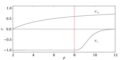
Figure 19: Radial characteristic speeds in ingoing Eddington–Finkelstein coordinates with a hyperboloidal layer attached. The dashed vertical red line depicts the interface to the layer at $I=8$. Null infinity is at the coordinate location $S=12$. These parameters are also used in the numerical simulations.

The radial characteristic speeds read

$$c_{+}=\frac{\rho-2M}{\rho+2M},$$

$$c_{-}=-\Omega^{2}\frac{(\rho-2M)(\rho-2M\Omega)}{2L\rho(\rho-2M)+\Omega^{2}(\rho+2M)(\rho-2M\Omega)}.$$

The outgoing speed $c_{+}$ has the same form as in iEF coordinates. Consequently, it vanishes at the event horizon $r=\rho=2M$. Similarly, the ingoing speed $c_{-}$ vanishes at null infinity, $\rho=S$ where $\Omega=0$. Figure 19 shows the radial characteristic speeds in these coordinates. The conformal diagram of the iEF foliation with a hyperboloidal layer is depicted in Fig. 20.

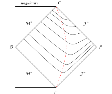
Figure 20: Conformal diagram of an ingoing Eddington–Finkelstein foliation with a hyperboloidal layer. The dashed red line corresponds to the interface. For visualization we have chosen $I=3$ and $S=4$. For the numerical computations we set $I=8$ and $S=12$ as in Fig. 19.

In the hyperboloidal layer we solve the conformally transformed scalar wave equation (1) that reads Wald (1984)

$$\Box\Phi-\frac{1}{6}R\,\Phi=\Omega^{-3}S(x),$$ (23)

where $\Phi=\phi/\Omega$ and $R$ is the Ricci scalar of the conformal background. The divisions by the conformal factor do not pose any difficulty because the scalar field falls off suitably and the source has compact support.

Appendix B Green function in geometrical optics

The numerical solutions presented in Sec. III can be regarded as approximations to the Green function for the scalar wave equation (1). We derive here, for the first time to our knowledge, the scalar Green function in Schwarzschild spacetime in the geometrical optics limit, which is used in the main text to compare numerical data with analytical approximations and to explain the fourfold cycle and the profiles of the caustic echoes. See Hartmann (2009) for a review of the geometrical optics limit in the field of optics.

In Schwarzschild spacetime there exists a time-like Killing vector, $\partial_{t}$, that allows for the Green function to be decomposed into frequency modes via

$$G(x,x^{\prime})=\int_{-\infty}^{\infty}\frac{d\omega}{2\pi}\,e^{-i\omega(t-t^{\prime})}G(\omega;{\bf x},\bf{x}^{\prime}).$$ (24)

In the frequency domain, using coordinates in which $g^{ti}=0$, the Green function equation (3) becomes a Helmholtz equation

$$\Delta G(\omega;{\bf x},{\bf x}^{\prime})+\omega^{2}u^{2}({\bf x})G(\omega;{\bf x},{\bf x}^{\prime})=0,$$ (25)

where $\Delta\equiv g^{ij}\nabla_{i}\nabla_{j}$ is the curved space Laplacian (with $i,j=1,2,3$), and we assume that ${\bf x}\neq{\bf x}^{\prime}$ so that the Dirac delta distribution in (3) vanishes. The function $u({\bf x})$ is defined by

$$u^{2}({\bf x})=-g^{tt}({\bf x}).$$ (26)

In standard Schwarzschild coordinates $u^{2}({\bf x})=1-\tfrac{2M}{r}$.

In the geometrical optics limit, the frequency of the mode approaches infinity (the wavelength of the mode is much smaller than the background curvature scale). We make the following ansatz for the asymptotic expansion of the Green function,

$$G(\omega;{\bf x},{\bf x}^{\prime})\sim\sum_{n=0}^{\infty}\frac{A_{n}({\bf x},{\bf x}^{\prime})}{(i\omega)^{n}}\,e^{i\omega T({\bf x},{\bf x}^{\prime})}.$$ (27)

Here, $T({\bf x},{\bf x}^{\prime})$ is called the eikonal and its level surfaces are surfaces of constant phase, called wavefronts. The covector $\nabla_{i}T$ is everywhere normal to this surface. Note that this ansatz is not covariant as time is a preferred direction. This may seem undesirable but our static observers measuring the field, as in Fig. 2, are Killing observers. Additionally, the geometrical optics approximation emphasizes time over space via the assumption of only high-frequencies contributing to the field. Hence, the lack of manifest covariance is suitable for our purposes.

Different level surfaces correspond to wavefronts with different phases of the Green function. We may thus parameterize these wavefronts by the phase, which is an affine parameter denoted by $\varphi$. As the field increases phase, and thus evolves forward in time, one moves from one wavefront to the next. This motion can be regarded as a mapping that allows one to identify paths, or rays, that connect specific points on different wavefronts. The Green function in (27) thus causally propagates points from one wavefront to another (Fig. 21). This viewpoint will be useful below.

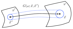
Figure 21: The retarded Green function as a mapping from a wavefront with phase $\varphi^{\prime}$ to a wavefront with phase $\varphi>\varphi^{\prime}$.

Substituting the leading order term of the sum in (27) into (25) and equating like powers of $\omega$ gives the following set of equations for the eikonal $T({\bf x},{\bf x}^{\prime})$ and the leading order amplitude $A_{0}({\bf x},{\bf x}^{\prime})$,

$$\nabla_{i}T\nabla^{i}T =u^{2}({\bf x})$$ (28)

$$2\nabla_{i}A_{0}\nabla^{i}T =-A_{0}\Delta T.$$ (29)

The first equation is called the eikonal equation and the second is called the transport equation. We will solve these equations in turn.

The solution to the eikonal equation (28) can be found by first defining a momentum vector $p_{i}\equiv\nabla_{i}T({\bf x})$, which is normal to the wavefront so that the eikonal equation reads ${\bf p}^{2}=u^{2}({\bf x})$. This defines a Hamiltonian for the rays connecting one wavefront to another

$$H=\frac{1}{2}\big{(}p_{i}p_{j}g^{ij}({\bf x})-u^{2}({\bf x})\big{)}.$$ (30)

The Hamiltonian vanishes when the eikonal equation is satisfied. Hamilton’s equations give

$$\frac{dx^{i}}{d\varphi} =p^{i}=\nabla^{i}T({\bf x})$$ (31)

$$\frac{Dp_{i}}{d\varphi} =\frac{1}{2}\nabla_{i}u^{2}({\bf x})$$ (32)

where $D/d\varphi=(dx^{i}/d\varphi)\nabla_{i}$ is the covariant parameter derivative along a trajectory with coordinates $x^{i}(\varphi)$ (i.e., a ray). Solving these ray equations thus amounts to solving the eikonal equation.

The square of the ray’s velocity is

$$\frac{dx^{i}}{d\varphi}\frac{dx_{i}}{d\varphi}=\nabla_{i}T\nabla^{i}T=u^{2}({\bf x})=-g^{tt}({\bf x}).$$ (33)

Collecting all terms on one side and multiplying by $d\varphi^{2}$ yields

$$g^{tt}({\bf x})d\varphi^{2}+g^{ij}({\bf x})dx_{i}dx_{j}=0.$$ (34)

Identifying $dx^{0}=dt=u^{2}({\bf x})d\varphi$, we see that the rays in the geometrical optics limit are null because $dx^{\mu}dx_{\mu}=0$. The solution to the eikonal equation thus amounts to solving for the trajectories of the null rays, which is equivalent to solving the geodesic equation for two light-like separated points, one on each wavefront.

Next, we solve the transport equation (29). Dividing both sides by $A_{0}$, noting that $\Delta T=\nabla_{i}\dot{x}^{i}(\varphi)$, and $\nabla^{i}T\nabla_{i}=D/d\varphi$ (from (31)) yields

$$\frac{d\ln A_{0}^{-2}}{d\varphi}=\nabla_{i}\dot{x}^{i}.$$ (35)

If an infinitesimal area on the wavefront centered at ${\bf x}^{\prime}\equiv{\bf x}(\varphi^{\prime})$ is evolved along the null geodesics to phase $\varphi>\varphi^{\prime}$ then the subsequent evolution can be viewed as a change of variable since ${\bf x}\equiv{\bf x}(\varphi)$ depends on the “initial data” at ${\bf x}^{\prime}$ and implies the coordinate transformation ${\bf x}={\bf x}(\varphi;{\bf x}^{\prime})$. The Jacobian relating these areas is

$$J({\bf x},{\bf x}^{\prime})=\frac{\partial(x^{0}\cdots x^{3})}{\partial(x^{\prime}{}^{0}\cdots x^{\prime}{}^{3})}={\rm det}M=e^{{\rm Tr}\ln M},$$ (36)

where the matrix $M$ has components $M^{i}{}_{j}=\partial x^{i}/\partial x^{\prime}{}^{j}$. Taking the parameter derivative of the Jacobian gives

$$\frac{dJ}{d\varphi}={} J\frac{\partial x^{\prime}{}^{i}}{\partial x^{j}}\frac{\partial\dot{x}^{j}}{\partial x^{\prime}{}^{i}}=J\frac{\partial x^{\prime}{}^{i}}{\partial x^{j}}\frac{\partial\dot{x}^{j}}{\partial x^{k}}\frac{\partial x^{k}}{\partial x^{\prime}{}^{i}}=J\frac{\partial\dot{x}^{i}}{\partial x^{i}}.$$ (37)

Using $\partial_{i}\dot{x}^{i}=\nabla_{i}\dot{x}^{i}-\Gamma^{i}_{i\alpha}\dot{x}^{\alpha}$ and

$$\Gamma^{i}_{i\alpha}\dot{x}^{\alpha}={} \Gamma^{i}_{it}+\Gamma^{i}_{ij}\dot{x}^{j}=\dot{x}^{j}\partial_{j}\ln\sqrt{h}$$

$$={} \frac{d}{d\varphi}\ln\sqrt{h}$$ (38)

where $h$ is the determinant of the spatial metric $g_{ij}$, we obtain from (35)

$$\frac{d\ln A_{0}^{-2}}{d\varphi}=\nabla_{i}\dot{x}^{i}=\frac{d}{d\varphi}\big{(}J\sqrt{h}\big{)}.$$ (39)

This has the solution

$$A_{0}({\bf x},{\bf x}^{\prime})=A_{0}({\bf x}^{\prime},{\bf x}^{\prime\prime})\left[\frac{J({\bf x}^{\prime},{\bf x}^{\prime\prime})}{J({\bf x},{\bf x}^{\prime})}\frac{\sqrt{h({\bf x}^{\prime})}}{\sqrt{h({\bf x})}}\right]^{1/2},$$ (40)

provided that ${\bf x}={\bf x}(\varphi)$ has not passed through any caustics and where $A_{0}({\bf x}^{\prime},{\bf x}^{\prime\prime})$ is initial amplitude (${\bf x}^{\prime\prime}$ is either a point on an earlier wavefront or can be equal to ${\bf x}^{\prime}$ in which case $J({\bf x}^{\prime},{\bf x}^{\prime})=1$). Hence, the amplitude of the wave at phase $\varphi^{\prime}$ for a given infinitesimal area around the point ${\bf x}^{\prime}={\bf x}(\varphi^{\prime})$ on the wavefront will evolve along the null ray to ${\bf x}={\bf x}(\varphi)$ with phase $\varphi>\varphi^{\prime}$ according to (40). Notice that the amplitude at ${\bf x}$ depends on the expansion or contraction of the infinitesimal area element on the wavefront during its evolution. This is equivalently described by the expansion or contraction of a congruence of null geodesics connecting ${\bf x}^{\prime}$ and ${\bf x}$. When the ray passes through a caustic the Jacobian $J({\bf x},{\bf x}^{\prime})$ changes sign relative to $J({\bf x}^{\prime},{\bf x}^{\prime\prime})$. We will say more about this in Appendix C.

Assuming that the ray has not passed through any caustics, we may reconstruct the time-domain Green function in (24) using (27) and (40) to find at leading order in $1/\omega$,

$$G(x,x^{\prime})\sim{} A_{0}({\bf x},{\bf x}^{\prime})\left[\frac{J({\bf x}^{\prime},{\bf x}^{\prime\prime})}{J({\bf x},{\bf x}^{\prime})}\frac{\sqrt{h({\bf x}^{\prime})}}{\sqrt{h({\bf x})}}\right]^{1/2}$$

$$\times{\rm Re}\int_{-\infty}^{\infty}\frac{d\omega}{2\pi}e^{-i\omega(t-t^{\prime}-T({\bf x},{\bf x}^{\prime}))},$$ (41)

where we take the real part of the integral because the field in the time domain is real valued. The evaluation of the integral gives

$$G(x,x^{\prime})\propto\delta\big{(}t-t^{\prime}-T({\bf x},{\bf x}^{\prime})\big{)}.$$ (42)

Hence, the geometrical optics approximation yields a contribution to the Green function whenever the time difference between $x^{\prime}$ and $x$ satisfies $t-t^{\prime}=T({\bf x},{\bf x}^{\prime})$, which is just the time it takes for a null geodesic to connect these two points.

Finally, we note that the remaining amplitudes $A_{n}({\bf x},{\bf x}^{\prime})$ in (27) can be determined through a recursion relation (for $n\geq 0$),

$$2\nabla^{i}T\nabla_{i}A_{n+1}+A_{n+1}\Delta T=-\Delta A_{n},$$ (43)

which follows from substituting (27) into (25) and setting the coefficients of each power of $\omega$ to zero. With $A_{0}$ known from (40) and the rays found by solving the null geodesic equation, we have the Schwarzschild Green function in the geometrical optics limit. The rays are null at all orders of $1/\omega$. Hence, the geometrical optics limit is inapplicable to the propagation into the null cone of ${\bf x}^{\prime}$ and thus ignores backscattering off the background curvature.

Appendix C Hilbert transform through a caustic

In Appendix B we solved the transport equation (29) for the field’s amplitude in the geometrical optics limit. The solution (40) assumes that the quantity under the radical is positive. However, if ${\bf x}={\bf x}(\varphi)$ evolves through a caustic then the Jacobian (36) changes sign. We show in Fig. 22 a cartoon of a wavefront area element as it passes through a generic caustic.

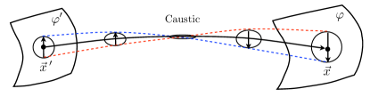
Figure 22: A cartoon of the change in orientation of an infinitesimal area element on the wavefront’s spatial section as it passes through a caustic in Schwarzschild spacetime. Only one dimension of the area element is compressed.

The sign change of the Jacobian through a caustic implies a purely imaginary amplitude in (40). Hence, the amplitude changes phase by $\pm\pi/2$ through a caustic Gouy (1890); Hartmann (2009). The sign of the phase shift is determined by matching to the full solution from numerical simulations. It cannot be computed within the geometrical optics approximation because the latter breaks down at caustics (where $J({\bf x},{\bf x}^{\prime})=0$ and $A({\bf x},{\bf x}^{\prime})$ becomes singular).

After some trial and error, we find that the phase of (40) when passing through one caustic is given by

$$\exp\left(-\frac{i\pi}{2}{\rm sgn}(\omega)\right).$$ (44)

For positive frequencies the phase is $-i$ while for negative frequencies it is $+i$. The frequency-dependence in (44) is needed for the reconstruction of the time-domain Green function in the geometrical optics limit. Computing (24), upon substituting the leading order term of the $1/\omega$ expansion from (27), gives

$$G(x,x^{\prime})\sim{} \big{|}A_{0}({\bf x}^{\prime},{\bf x}^{\prime\prime})\big{|}\left[\bigg{|}\frac{J({\bf x}^{\prime},{\bf x}^{\prime\prime})}{J({\bf x},{\bf x}^{\prime})}\bigg{|}\sqrt{\frac{h({\bf x}^{\prime})}{h({\bf x})}}\,\right]^{1/2}$$

$$\times\theta\big{(}t-t^{\prime}-T_{0}({\bf x},{\bf x}^{\prime})\big{)}$$

$$\times{\rm Re}\int_{-\infty}^{\infty}\frac{d\omega}{2\pi}\,e^{-i\omega(t-t^{\prime}-T_{1}({\bf x},{\bf x}^{\prime}))}e^{-\frac{i\pi}{2}{\rm sgn}(\omega)},$$ (45)

where we have explicitly taken the real part as in (41), $T_{N}({\bf x},{\bf x}^{\prime})$, with $N=0,1$, is the eikonal for the null geodesic connecting ${\bf x}$ and ${\bf x}^{\prime}$ and passing through $N$ caustics, and the step function ensures causality (namely, that the $T_{1}$ eikonal is larger than $T_{0}$). The frequency integral gives

$$-\frac{1}{\pi\big{(}t-t^{\prime}-T_{1}({\bf x},{\bf x}^{\prime})\big{)}}.$$ (46)

As discussed in Sec. III.3, when the Green function is convolved with the source $S(x)$ from (2) one finds that passing through one caustic transforms the field from a Gaussian profile to that of a Dawson’s integral (or “Dawsonian”), which is the convolution of (46) with the source $S(x)$ Duoandikoetxea (2008). Hence, the choice given in (44) for the sign of the root of $A_{0}^{2}({\bf x},{\bf x}^{\prime})$ in (40) is justified through this matching calculation.

Comparing (46) to (42) we note that the latter has support only along the null ray connecting ${\bf x}$ and ${\bf x}^{\prime}$ while the former has a much broader domain of support. Both expressions are singular on null rays (where $t-t^{\prime}=T_{0}({\bf x},{\bf x}^{\prime})$ or $T_{1}({\bf x},{\bf x}^{\prime})$), but (46) does not vanish in the forward light cone thus adding to the tail. Passing through one caustic causes the sharp delta distribution to become smeared out into the future null cone of ${\bf x}^{\prime}$ beyond the caustic.

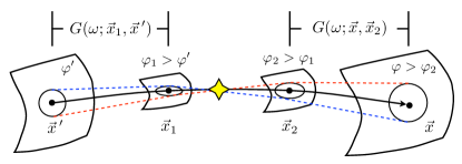
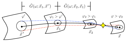
Figure 23: Top: The retarded Green function in the geometrical optics limit for a null ray connecting ${\bf x}^{\prime}$ to ${\bf x}$ through a single caustic. The geometrical optics approximation breaks down at the caustic (yellow star) but is valid from the wavefronts with phase $\varphi^{\prime}$ to $\varphi_{1}>\varphi^{\prime}$ and from the wavefront with phase $\varphi_{2}$ to $\varphi>\varphi_{2}$. Bottom: In Maslov’s theory the caustic is displaced by a phase space canonical transformation yielding a related Green function that allows for propagating the wavefront with phase $\varphi^{\prime}$ directly to $\varphi_{2}$ via $\varphi_{1}$.

The frequency integral in (45) is the Hilbert transform of $\delta(t-t^{\prime}-T_{1}({\bf x},{\bf x}^{\prime}))$. For a function $f(t)$, the Hilbert transform in the frequency domain is defined as

$$H[f(t)]=\int_{-\infty}^{\infty}\frac{d\omega}{2\pi}\,\hat{f}(\omega)e^{-i\pi/2\,{\rm sgn}(\omega)},$$ (47)

where $\hat{f}(\omega)$ is the Fourier transform of $f(t)$. The effect of the Hilbert transform is to shift the phase of $\hat{f}(\omega)$ by $-\pi/2$. Two applications of the Hilbert transform gives $H_{2}[f(t)]\equiv H[H[f(t)]]=-f(t)$, which is a $-\pi$ phase shift of $f(t)$. Four applications of the Hilbert transform gives back the function itself,

$$H_{4}[f(t)]=f(t).$$ (48)

Thus, the Hilbert transform explains the fourfold cycle of the retarded Green function through caustics. This allows us to generalize (45) to include all the null rays that connect ${\bf x}$ and ${\bf x}^{\prime}$ (of which there are infinitely many for a Schwarzschild black hole Hasse and Perlick (2002)),

$$G(x,x^{\prime})\sim{} \sum_{N=0}^{\infty}\big{|}A_{0}({\bf x}^{\prime},{\bf x}^{\prime\prime})\big{|}\left[\bigg{|}\frac{J({\bf x}^{\prime},{\bf x}^{\prime\prime})}{J({\bf x},{\bf x}^{\prime})}\bigg{|}\sqrt{\frac{h({\bf x}^{\prime})}{h({\bf x})}}\,\right]^{1/2}$$

$$\times\theta(t-t^{\prime}-T_{N-1}({\bf x},{\bf x}^{\prime}))\,{\rm Re}\int_{-\infty}^{\infty}\frac{d\omega}{2\pi}$$

$${\hskip 18.06749pt}\times e^{-i\omega(t-t^{\prime}-T_{N}({\bf x},{\bf x}^{\prime}))}e^{-\frac{i\pi N}{2}{\rm sgn}(\omega)},$$ (49)

where $T_{-1}({\bf x},{\bf x}^{\prime})\equiv 0$. This formula can be written more succinctly as

$$G(x,x^{\prime})\sim{} \sum_{N=0}^{\infty}\big{|}A_{0}({\bf x},{\bf x}^{\prime})\big{|}\,\theta(t-t^{\prime}-T_{N-1}({\bf x},{\bf x}^{\prime}))$$

$${\hskip 18.06749pt}\times{\rm Re}\big{\{}H_{N}\big{[}\delta(t-t^{\prime}-T_{N}({\bf x},{\bf x}^{\prime}))\big{]}\big{\}},$$ (50)

where $T_{N}({\bf x},{\bf x}^{\prime})$ is the eikonal for the null geodesic that passes through $N$ caustics and $H_{N}$ denotes the Hilbert transform applied $N$ times to its argument.

As mentioned at the beginning of this Appendix, the geometrical optics approximation breaks down at caustics where many points of a wavefront get mapped to the same (caustic) point. The Jacobian $J({\bf x},{\bf x}^{\prime})$ vanishes and the amplitude of the field $A_{0}({\bf x},{\bf x}^{\prime})$ diverges as $J({\bf x},{\bf x}^{\prime})^{-1/2}$. The geometrical optics approximation is valid only between successive caustics. One may use the geometrical optics Green function to evolve wavefronts before and after a caustic but not through (Fig. 23).

Remarkably, the breakdown of geometrical optics at a caustic can be averted (or rather, displaced) using Maslov’s theory Maslov (1965, 1972); Kravtsov (1968). A caustic arises due to singularities in the projection of some higher dimensional space to a lower one. In our case, the higher dimensional space is the phase space of null rays (with coordinates $({\bf x},{\bf p})$) wherein the null rays follow trajectories with coordinates $({\bf x}(\varphi),{\bf p}(\varphi))$ that do not intersect because their evolution is Hamiltonian [see (30)].

Instead of forming the asymptotic series in $1/\omega$ for $G(\omega;{\bf x},{\bf x}^{\prime})$, Maslov’s idea is to form the series for its Fourier transform with respect to at least one of its spatial coordinates. Then the Fourier transform operates as a canonical transformation in phase space. When the new momentum variables are projected out, caustics form at different locations than previously. This change of caustic location allows us, in principle, to construct a well-defined asymptotic series for the geometrical optics approximation of the Green function by using Maslov’s theory whenever a caustic is about to be encountered (Fig. 23). In this way, one may be able to derive directly the phase shift through a caustic in (44) without recourse to a matching argument. The application of Maslov’s theory is outside the scope of this paper.

References

- (1) A. Ori, On the structure of the Green’s function beyond the caustics: theoretical findings and experimental verification, http://physics.technion.ac.il/~amos/acoustic.pdf.
- Ames and Thorne (1968) W. L. Ames and K. S. Thorne, Astrophys. J. 151, 659 (1968).
- Goebel (1972) C. J. Goebel, Astrophysical Journal 172, L95 (1972).
- Casals et al. (2009) M. Casals, S. Dolan, A. C. Ottewill, and B. Wardell, Phys.Rev. D79, 124044 (2009), eprint 0903.5319.
- Casals et al. (2010) M. Casals, S. Dolan, A. C. Ottewill, and B. Wardell (2010), eprint 1003.5790.
- Casals and Nolan (2012) M. Casals and B. C. Nolan, Phys.Rev. D86, 024038 (2012), eprint 1204.0407.
- Dolan and Ottewill (2011) S. R. Dolan and A. C. Ottewill, Phys.Rev. D84, 104002 (2011), eprint 1106.4318.
- Dolan and Ottewill (2009) S. R. Dolan and A. C. Ottewill, Class.Quant.Grav. 26, 225003 (2009), eprint 0908.0329.
- Harte and Drivas (2012) A. I. Harte and T. D. Drivas, Phys.Rev. D85, 124039 (2012), eprint 1202.0540.
- (10) SpEC: Spectral Einstein Code. http://www.black-holes.org/SpEC.html.
- Zenginoglu (2008) A. Zenginoglu, Class. Quant. Grav. 25, 145002 (2008), eprint 0712.4333.
- Zenginoglu (2011a) A. Zenginoglu, J. Comput. Phys. 230, 2286 (2011a), eprint 1008.3809.
- vid (a) Caustic Echoes from a Nonrotating Black Hole, http://www.youtube.com/watch?v=Pe8sRjqtldQ.
- Andersson (1994) N. Andersson, Class.Quant.Grav. 11, 3003 (1994).
- Decanini et al. (2010) Y. Decanini, A. Folacci, and B. Raffaelli, Phys.Rev. D81, 104039 (2010), eprint 1002.0121.
- Stewart (1989) J. M. Stewart, Proc. R. Soc. Lond. A 424, 239 (1989).
- Ferrari and Mashhoon (1984) V. Ferrari and B. Mashhoon, Phys.Rev. D30, 295 (1984).
- Iyer and Will (1987) S. Iyer and C. M. Will, Phys.Rev. D35, 3621 (1987).
- Cardoso et al. (2009) V. Cardoso, A. S. Miranda, E. Berti, H. Witek, and V. T. Zanchin, Phys.Rev. D79, 064016 (2009), eprint 0812.1806.
- Gouy (1890) C. R. Gouy, C. R. Acad. Sci. Paris 110, 1251 (1890).
- Hartmann (2009) R. Hartmann, Theoretical Optics: An Introduction (Wiley-VCH, 2009).
- Duoandikoetxea (2008) J. Duoandikoetxea, J. Math. Anal. Appl. 347, 592 (2008).
- Kay and Keller (1954) I. Kay and J. B. Keller, Journal of Applied Physics 25, 876 (1954).
- Price (1972) R. H. Price, Phys.Rev. D5, 2419 (1972).
- Gundlach et al. (1994) C. Gundlach, R. H. Price, and J. Pullin, Phys.Rev. D49, 883 (1994), eprint gr-qc/9307009.
- Perlick (2010) V. Perlick, Living Rev.Rel. (2010), eprint 1010.3416.
- Hasse and Perlick (2002) W. Hasse and V. Perlick, Gen.Rel.Grav. 34, 415 (2002), eprint gr-qc/0108002.
- Bizon and Rostworowski (2010) P. Bizon and A. Rostworowski, Phys.Rev. D81, 084047 (2010), eprint 0912.3474.
- Casals and Ottewill (2012) M. Casals and A. C. Ottewill (2012), eprint 1205.6592.
- Hadamard (1923) J. Hadamard, Lectures on Cauchy’s Problem in Linear Partial Differential Equations (Yale University Press, New Haven, 1923).
- Poisson et al. (2011) E. Poisson, A. Pound, and I. Vega, Living Rev.Rel. 14, 7 (2011), eprint 1102.0529.
- Ottewill and Wardell (2011) A. C. Ottewill and B. Wardell, Phys.Rev. D84, 104039 (2011), eprint 0906.0005.
- Taylor et al. (2010) N. W. Taylor, L. E. Kidder, and S. A. Teukolsky, Phys.Rev. D82, 024037 (2010), eprint 1005.2922.
- Lau et al. (2009) S. R. Lau, H. P. Pfeiffer, and J. S. Hesthaven, Communications in Computational Physics 6, 1063 (2009), eprint 0808.2597.
- Lu and Yang (2011) J. Lu and X. Yang, Commun. Math. Sci. 9, 663 (2011), eprint 1010.1968.
- Candes et al. (2009) E. Candes, L. Demanet, and L. Ying, SIAM Multiscale Model. Simul. 7-4, 1727 (2009).
- Teo (2003) E. Teo, General Relativity and Gravitation 35, 1909 (2003).
- Yang et al. (2012) H. Yang, D. A. Nichols, F. Zhang, A. Zimmerman, and Y. Chen (2012), in preparation.
- vid (b) Caustic Echoes from a Rotating Black Hole, http://www.youtube.com/watch?v=iEA31IL1mFI.
- Arnold (1984) V. I. Arnold, Catastrophe theory (Berlin: Springer, 1984).
- Zenginoglu (2011b) A. Zenginoglu, Phys. Rev. D83, 127502 (2011b), eprint 1102.2451.
- Jasiulek (2012) M. Jasiulek, Class.Quant.Grav. 29, 015008 (2012), eprint 1109.2513.
- Bernuzzi et al. (2011) S. Bernuzzi, A. Nagar, and A. Zenginoglu, Phys.Rev. D84, 084026 (2011), eprint 1107.5402.
- Zenginoglu and Khanna (2011) A. Zenginoglu and G. Khanna, Phys.Rev. X1, 021017 (2011), eprint 1108.1816.
- Wald (1984) R. M. Wald, General relativity (The University of Chicago Press, Chicago, 1984), ISBN 0-226-87032-4 (hardcover), 0-226-87033-2 (paperback).
- Maslov (1965) V. P. Maslov, Theory of Perturbations and Asymptotic Methods (Izd. MGU, Moscow, USSR, 1965), (in Russian).
- Maslov (1972) V. P. Maslov, Théorie des Perturbations et Méthodes Asymptotiques (Dunod, Paris, France, 1972).
- Kravtsov (1968) Y. A. Kravtsov, Soviet Physics-Acoustics 14, 1 (1968).