Overview of Bohmian Mechanics

Abstract

This chapter provides a fully comprehensive overview of the Bohmian formulation of quantum phenomena. It starts with a historical review of the difficulties found by Louis de Broglie, David Bohm and John Bell to convince the scientific community about the validity and utility of Bohmian mechanics. Then, a formal explanation of Bohmian mechanics for non-relativistic single-particle quantum systems is presented. The generalization to many-particle systems, where correlations play an important role, is also explained. After that, the measurement process in Bohmian mechanics is discussed. It is emphasized that Bohmian mechanics exactly reproduces the mean value and temporal and spatial correlations obtained from the standard, i.e., ‘orthodox’, formulation. The ontological characteristics of the Bohmian theory provide a description of measurements in a natural way, without the need of introducing stochastic operators for the wavefunction collapse. Several solved problems are presented at the end of the chapter giving additional mathematical support to some particular issues. A detailed description of computational algorithms to obtain Bohmian trajectories from the numerical solution of the Schrödinger or the Hamilton–Jacobi equations are presented in an appendix. The motivation of this chapter is twofold. First, as a didactic introduction of the Bohmian formalism which is used in the subsequent chapters. Second, as a self-contained summary for any newcomer interested in using Bohmian mechanics in their daily research activity.

I Preface first edition

New cutting edge ideas come from outside of the main stream

Most of our collective activities are regulated by other people who decide whether they are well done or not. One has to learn some arbitrary symbols to write understandable messages, or to read those from others. Human rules over collective activities govern the evolution of our culture. On the contrary, natural systems, from atoms to galaxies, evolve independently of the human rules. Men cannot modify physical laws. We can only try to understand them. Nature itself judges, through experiments, whether a plausible explanation for some natural phenomena is correct or not. Nevertheless, in forefront research where the unknowns start to become understandable, the new knowledge is still unstable, somehow immature. It is supported by few experimental evidences or the evidences are still subjected to different interpretations. Certainly, novel research grows up closely tied to the economical, sociological or historical circumstances of the involved researchers. A period of time is needed in order to distil new knowledge, separating pure scientific arguments from cultural influences.

The past and the present status of Bohmian mechanics cannot be understood without these cultural considerations. The Bohmian formalism was proposed by Louis de Broglie even before the standard, that is Copenhagen, explanation of quantum phenomena was established. Bohmian mechanics provides an explanation of quantum phenomena in terms of particles guided by waves. One object cannot be a wave and a particle simultaneously, but two can. Specially, if one of the objects is a wave and the other is a particle. Unfortunately, Louis de Broglie, himself, abandoned these ideas. Later, in the fifties, David Bohm clarified the meaning and applications of this original explanation of quantum phenomena. Bohmian mechanics agrees with all non-relativistic quantum experiments done up to now. However, it remains almost ignored by most of the scientific community. In our opinion, there are no scientific arguments to support its marginal status, but only cultural reasons. One of the motivations for writing this book is helping in the maturing process that Bohmian mechanics still needs.

Certainly, the distilling process of Bohmian mechanics is being quite slow. Anyone interested enough to walk this causal road of quantum mechanics can be easily confused by many misleading signposts that have been raised in the scientific literature, not only by its detractors, but unfortunately very often also by some of its advocates. Following opinions from other reputed physicists (we are easily persuaded by those scientists with authority) is far from being a proper scientific strategy.

In any case, since the mathematical structure of Bohmian mechanics is quite simple, it can be easily learned by anyone with only a basic knowledge of classical and quantum mechanics who makes the necessary effort to build his own scientific opinion based on logical deductions, free from cultural influences. The introductory chapter of this book, including a thorough list of exercises and easily programmable codes, provides a reasonable and objective source of information in order to achieve this later goal, even for undergraduate students.

Curiously, the fact that Bohmian mechanics is ignored and remains mainly unexplored is an attractive feature for some adventurous scientists. They know that very often new cutting edge ideas come from outside of the main stream and find in Bohmian mechanics a useful tool in their research activity. On the one hand, it provides an explanation of quantum mechanics, in terms of trajectories, that results to be very useful in explaining the dynamics of quantum systems, being thus also a source of inspiration to look for novel quantum phenomena. On the other hand, since it provides an alternative mathematical formulation, Bohmian mechanics offers new computational tools to explore physical scenarios that presently are computationally inaccessible, such as many particle solutions of the Schrödinger equation. In addition, Bohmian mechanics sheds light on the limits and extensions of our present understanding of quantum mechanics towards other paradigms such as relativity or cosmology, where the internal structure of Bohmian mechanics in terms of well-defined trajectories is very attractive. With all these previous motivations in mind, this book provides nine chapters (apart from the introduction in the first chapter) with practical examples showing how Bohmian mechanics helps us in our daily research activity.

Obviously, there are other books focused on Bohmian mechanics. However, many of them are devoted to the foundations of quantum mechanics emphasizing the difficulties or limitations of the Copenhagen interpretation for providing an ontological description of our world. On the contrary, this book is not focus on the foundations of quantum mechanics, but on the discussion about the practical application of the ideas of de Broglie and Bohm to understand and compute the quantum world. Several examples of such practical applications written by leading experts in different fields, with an extensive updated bibliography, are provided here. The book, in general, is addressed to students in physics, chemistry, electrical engineering, applied mathematics, nanotechnology, as well as to both theoretical and experimental researchers who seek new computational and interpretative tools for their everyday research activity. We hope that the newcomers to this causal explanation of quantum mechanics will use Bohmian mechanics in their research activity so that Bohmian mechanics will become more and more popular for the broad scientific community. If so, we expect that, in the near future, Bohmian mechanics will be taught regularly at the Universities, not as the unique and revolutionary way of understanding quantum phenomena, but as an additional and useful interpretation of all quantum phenomena in terms of quantum trajectories. In fact, Bohmian mechanics has the ability of removing most of the mysteries of the Copenhagen interpretations and, somehow, simplifying (or demystifying) quantum mechanics. We will be very glad if this book can contribute to shorten the time needed to achieve all these goals.

Finally, we want to acknowledge many different people that has allowed us to embark into and successfully finish this book project. First of all, Alfonso Alarcón and Albert Benseny who became involved in the book project from the very beginning, as two additional editors. We also want to thank the rest of the authors of the book for accepting our invitation to participate in this project and writing their chapters according to the general spirit of the book. Due to page limitations, only nine examples of practical applications of Bohmian mechanics in forefront research activity are presented in this book. Therefore, we want to apologize to many other researchers who could have certainly been also included in the book. We also want to express our gratitude to Pan Stanford Publishing for accepting our book project and for their kind attention during the publishing process.

II Preface second edition:

Quantum engineering: a giant with feet of clay

More than five years after the first edition of our book on applied Bohmian mechanics, our original motivations for writing it are still very present. Certainly, today, a lot of publicity about the abilities of the Bohmian theory is still needed among the scientific community. In fact, over these last few years, many research programs have been devoted to the so-called quantum engineering with the goal of developing new materials, new sensors, or new computing strategies based on pure quantum phenomena. Thus, this book can be understood as a promotional presentation on how the Bohmian theory, among others, can help in the design and development of such applications. However, Bohmian mechanics is not a mere computational tool in terms of quantum trajectories, but a complete and ontological theory that provides a consistent explanation on how Nature works. In this regard, this book can also be seen as a useful exercise to sincerely question our present understanding of the physical laws that govern the quantum world. After a bit of reflection on this point, many of us will probably conclude that our knowledge about the fundamentals of the quantum world are much more immature and imprecise than what we previously thought. In this sense, we want this book to be a warning on the the risks of constructing the new and exciting discipline of quantum engineering as a giant with feet of clay.

The beginning of the 20th century saw the first quantum revolution where novel and original theories were developed to understand unexpected non-classical phenomena. What determines the structure of the periodic table? Why are some materials metals and some dielectrics, while others behave like semiconductors? Nowadays, having established answers to these basic questions, a second quantum revolution is starting to take place, focusing on actively capitalizing on our quantum knowledge to alter the face of the physical world, developing a myriad of new quantum technologies. The difference between these two quantum revolutions is just the difference between science and engineering. The first revolution tried to properly understand our physical surroundings, the natural objects around us, while the second one intends to manipulate these surroundings to our own benefit. This is the typical evolution of most scientific disciplines. When scientific knowledge is mature enough, and the necessary technological means are available, engineers can use this knowledge for practical applications.

It is a common belief in our society that quantum theory, after more than a century, is ready to take a leap towards the engineering field. We have certainly outstanding technological means to manipulate quantum systems, even individual atoms, at the nanometer and femtosecond scales. Therefore, many national or international research organizations are focusing their programs towards the effective development of quantum technologies, trying to ensure that money spent on science has a direct impact on our society and its challenges for a better life. This is indeed a legitimate and compelling goal. However, is the quantum theory mature enough to blindly jump from science towards engineering? The pressure from society (in terms of research programs, grants, citing indices, etc.) is so effective that it forces most of the scientists to forget about the maturity of the quantum theory and just focus on (what really matters) the fast development of practical applications in the new and exciting field of quantum engineering.

We argue that the development of quantum engineering cannot be done at the price of forgetting the need for a deeper understanding of the physical laws governing the quantum world. One of the forgotten discussions by the new generation of quantum engineers is the measurement problem, which remains inside the backbone of the quantum theory. The measurement problem is manifested in the orthodox theory by its failure in explaining which physical interactions among particles constitute a measurement and which do not. In fact, there are many more examples of the immaturity of our quantum knowledge. Our inability to properly describe many-body systems due to their exponential complexity (the so-called many-body problem) makes that most of our understanding is based on a puerile single-particle description. We do not have a clear physical picture on the quantum-to-classical transition. What makes a quantum system to behave classically in some circumstances? The fact that there are several quantum theories which are empirically equivalent but radically different at the ontological level is a clear evidence of our bad understanding. The Copenhagen theory is the most extensively investigated and presently the one with more support among the scientific community. Others include spontaneous collapse theories or the many-worlds theory. The one studied in this book, Bohmian mechanics, provides a description of quantum phenomena by particles choreographed by the wave function. In general, neither of these theories is more mature than the orthodox one, but they remove the need of an observer, which relaxes some of the difficulties to understand the measurement at a quantum level. Some of these alternative theories are not free of problems, including the quantum-to-classical transition and the many-body problem, while others still need to be dealt with. We do not mean to imply that these alternative theories are better (how does one quantify better here?), but that there is still a lot of work needed to certify that our comprehension of the quantum world is unproblematic.

Let us try to exemplify the risks of developing quantum engineering alone without worrying on its fundamentals. In the orthodox theory, every time we make a measurement a random process occurs. But, as we do not really know what makes a physical interaction to be a measurement, we really do not know the origin of such randomness. In the Bohmian theory, for example, this randomness comes from an uncertainty in the initial position of the particles. With further efforts to clarify the quantum theories, we can perhaps achieve a better understanding of the origin of quantum randomness and then, the exciting new building of application developed along the new discipline of quantum cryptography, based on the unavoidable presence of such intrinsic quantum randomness, will simple melt as a giant with feet of clay. The reader can argue that there are a lot of scientific works supporting the actual status of quantum cryptography. Perhaps this particular warning is completely unfounded and quantum cryptography will certainly remain as robust as we know today. But, perhaps not. It is enlightening to remember here the theorem that John von Neumann stated in 1932 about the impossibility of explaining quantum mechanics with hidden variables (such as quantum trajectories). This theorem remained an unquestionable truth, and part of the essence of the quantum world, until David Bohm (with an explanation of quantum phenomena in terms of waves and particles) showed that the theorem was wrong (as its own preliminary assumptions precludes the existence of Bohmian trajectories). The curious spectacle is not that John von Neumann (an outstanding scientist in many disciplines) made a mistake in a theorem, but that the community (with the exception of Grete Hermann in 1935 that was totally ignored) blindly accepted the theorem for almost half a century.

There are many more examples which certify that our understanding of the quantum world is still immature. The wave function, the basic element in most theories, can be prepared for instance by forcing the quantum system into its ground state, but it cannot be directly measured in a single experiment. The wave function can be measured through a weak protocol, but also Bohmian velocities can be measured though such protocol. We do not even know what is really the wave function at the most fundamental level: a law? a field? a probability transporter?

In summary, the quantum world is so complicated that one century has not been enough for the scientific community to clearly elaborate an unproblematic description of the laws of quantum mechanics. We are not arguing here that research on quantum engineering needs to stop. Just the contrary. The development of the quantum engineering and the research on the foundations of the quantum theory have to evolve intimately connected to benefice from each other in achieving better practical applications and a deeper understanding of the quantum world. Otherwise, we will build a giant with feet of clay. We hope that the present book can be viewed as a modest contribution in both directions.

III Introduction

The beginning of the twentieth century brought surprising non-classical phenomena. Max Planck’s explanation of the black body radiation om.Planck-BlackBody , the work of Albert Einstein on the photoelectric effect om.Einstein-Photoelectric and the Niels Bohr’s model to account for the electron orbits around the nuclei om.bohr ; om.bohr2 ; om.bohr3 established what is now known as the old quantum theory. To describe and explain these effects, phenomenological models and theories were first developed, without rigorous justification. In order to provide a complete explanation for the underlying physics of such new non-classical phenomena, physicists were forced to abandon classical mechanics to develop novel, abstract and imaginative formalisms.

In 1924, Louis de Broglie suggested in his doctoral thesis that matter, apart from its intrinsic particle-like behavior, could exhibit also a wave-like one om.dB_AnnPhys . Three years later he proposed an interpretation of quantum phenomena based on non-classical trajectories guided by a wave field om.debroglie1927b . This was the origin of the pilot-wave formulation of quantum mechanics that we will refer as Bohmian mechanics to account for the following work of David Bohm om.bohm1952a ; om.bohm1952b . In the Bohm formulation, an individual quantum system is formed by a point particle and a guiding wave. Contemporanely, Max Born and Werner Heisenberg, in the course of their collaboration in Copenhagen with Niels Bohr, provided an original formulation of quantum mechanics without the need of trajectories om.Born1926 ; om.Heisenber1925 . This was the origin of the so-called Copenhagen interpretation of quantum phenomena and, since it is the most accepted formulation, it is basically the only one explained at most universities. Thus, it is also known as the orthodox formulation of quantum mechanics. In the Copenhagen interpretation, an individual quantum system exhibits its wave or its particle nature depending on the experimental arrangement.

The present status of Bohmian mechanics among the scientific community is quite marginal (the quantum chemistry community is an encouraging exception). Most researchers do not know about it or believe that is not fully-correct. There are others that know that quantum phenomena can be interpreted in terms of trajectories, but they think that this formalism cannot be useful in their daily research activity. Finally, there are few researchers, the authors of this book among them, who think that Bohmian mechanics is a useful tool to make progress in front-line research fields involving quantum phenomena.

The main (non-scientific) reason why still many researchers believe that there is something wrong with Bohmian mechanics can be illustrated with Hans Christian Andersen’s tale The Emperor’s new clothes. Two swindlers promise the Emperor the finest clothes that, as they tell him, are invisible to anyone who is unfit for their position. The Emperor cannot see the (non-existing) clothes, but pretends that he can for fear of appearing stupid. The rest of the people do the same. Advocates of the Copenhagen interpretation have attempted to produce impossibility proofs in order to demonstrate that Bohmian mechanics is incompatible with quantum phenomena om.impossibility_proofs . Most researchers, who are not aware of the incorrectness of such proofs, might conclude that there is some controversy with the Bohmian formulation of quantum mechanics and they prefer not to support it, for fear of appearing discordant. At the end of the tale, during the course of a procession, a small child cries out “the Emperor is naked!”. In the tale of quantum mechanics, David Bohm om.bohm1952a ; om.bohm1952b and John Bell om.Bell1987 were the first to exclaim to the scientific community “Bohmian mechanics is a correct interpretation of quantum phenomena that exactly coincides with the predictions of the orthodox interpretation!”.

III.1 What is a quantum theory

Albert Einstein, in the paper entitled “Physics and reality” einstein , pointed out the possibility of living in a bizarre world without comprehensible explanations for natural phenomena. He wrote: “The fact that [the world] is comprehensible is a miracle”. Similarly, Eugene Wigner wrote: “The unreasonable effectiveness of mathematics in the natural science ….is a wonderful gift which we neither understand nor deserve” wigner . Both reflections were inspired by the previous work of the German philosopher Immanuel Kant who wrote the very same idea almost two centuries before: “The eternal mystery of the world is its comprehensibility.”. Fortunately, it seems that we live in a comprehensible world.

Kant divided scientific knowledge into three categories: appearance, reality and theory. Appearance is the content of our sensory experience of natural phenomena, which is the empirical outcome of an experiment. Reality is what lies behind all natural phenomena. A theory is a human model that tries to mirror both appearance and reality. A useful theory might predict the outcome of an experiment in a laboratory or the observation of a phenomenon in Nature. Empiricists believe on experimental outcomes (what Kant called appearance) and refuse to speculate about a deeper reality. On the other hand, realists believe that good physical theories explain, or at least provide clues about, the reality of our comprehensible world. Most researchers are a combination of both stereotypes, with variable proportions.

As all human creations, there are successful and unsuccessful theories. When in 1864 James Clerk Maxwell conjectured that light was an electromagnetic vibration, it was believed that all waves had to vibrate in some medium. The medium in which light presumably travels was named luminiferous ether. During almost a century eminent scientists believed blindly on that concept. Nowadays, the luminiferous ether plays no role at all in modern physical theoriesom.herbert . The atomicity of matter is an example of a very successful theory. It was introduced by the British chemist John Dalton in 1808 to explain why some chemical substances need to combine in some fixed ratios. During one century it was thought that atoms were a crazy idea. Marcelin Berthelot said “who [has] ever seen a gas molecule or an atom?”, expressing the disdain that many chemists felt for the unseen atoms, which were inaccessible to experiments om.herbert . Even their defenders saw little hope of ever directly verifying the atomic hypothesis. Nowadays, the fact that everything is made of atoms is one of the most precious knowledge that we get on how Nature worksfeynmann , and their images are even routinely seen in the screens of scanning tunneling microscopes binning .

A quantum theory is a human explanation of quantum phenomena. All quantum theories have associated their own intangible reality. The so-called ontology of the theory. For example, the ontology of the Bohmian theory is very simple: everything is build by point particles guided (“choreographed”) by waves. The different quantum theories available today (Copenhagen, Bohmian, many worlds, spontaneous collapse, etc.) are indeed inspired by radically different realities, but all of them provide the same empirical predictions on quantum phenomena. In Kant’s words, all of them provide the same explanation of the appearance of our world. As we repeatedly stressed, up to know, in spite of many attempts, there is no experimental evidence that can discern between Bohmian and Copenhagen realities (ontologies).

In fact, for practical applications, even wrong theories can be very useful. Most natural phenomena that affect our ordinary life can be exclusively explained in terms of classical mechanics. However, today, we know that the reality behind the classical theory is wrong because it does not provide accurate predictions for some natural phenomena, like relativistic (with particles with high velocities) or quantum (atomistic dimensions) experiments. Surprisingly, the fact that the classical theory is a wrong theory does not demerit its extraordinary utility and our confidence on its predictions within its range of validity. The same is true for most physical theories at a practical level. Even if we could demonstrate in the future that either the Copenhagen or the Bohmian theories is wrong (or both), the practical utility of these theories in their range of validity would not dismiss.

III.2 How Bohmian mechanics helps

Although there is no experimental evidence against Bohmian mechanics, many researchers believe that Bohmian mechanics is not a useful tool to do research. In the words of Steven Weinberg, in a private exchange of letters with Sheldon Goldstein om.Weinberg : “In any case, the basic reason for not paying attention to the Bohm approach is not some sort of ideological rigidity, but much simpler — it is just that we are all too busy with our own work to spend time on something that doesn’t seem likely to help us make progress with our real problems.”.

The history of science seems to give credit to Weinberg‘s sentence. In spite of the controversies that have always been associated with the Copenhagen interpretation since its birth a century ago, its mathematical and computational machinery has enabled physicists, chemists and (quantum) engineers to calculate and predict the outcome of a vast number of experiments, while the contribution of Bohmian mechanics during the same period is much less significative. The differences are due to the fact that Bohmian mechanics remains mainly unexplored.

Contrarily to Weinberg’s opinion, we believe that Bohmian mechanics can help us make progress with our real problems. There are, at least, three clear reasons why one could be interested in studying quantum problems with Bohmian mechanics:

1. Bohmian explaining: Even when the Copenhagen mathematical machinery is used to compute observable results, the Bohmian interpretation ofently offers different interpretational tools. We can find descriptions of electron dynamics such as “an electron crosses a resonant tunneling barrier and interacts with another electron inside the well”. However, according to the orthodox theory, we can only talk about the properties of an electron (for example, its position) when we measure it. If we do not measure it, the electron has no property. Thus, an electron crossing a tunneling region is not rigorously supported within orthodox quantum mechanics, but it is within the Bohmian picture. Thus, in contrast to the Copenhagen theory, Bohmian mechanics allows for an easy visualization of quantum phenomena in terms of trajectories that has important demystifying or clarifying consequences. In fact, Bohmian mechanics allows for an unambiguous description of measured and unmeasured properties of particles (an electron crossing a tunneling barrier is a description of unmeasured properties). Bohmian mechanics provides a single-event description of the experiment, while Copenhagen quantum mechanics accounts for its statistical or ensemble explanation. We will present several examples in chapters 2 and 3 emphasizing all these points.
   

2. Bohmian computing: Although the predictions of the Bohmian interpretation reproduce the ones of the orthodox formulation of quantum mechanics, its mathematical formalism is different. In some systems, the Bohmian equations might provide better computational tools than the ones obtained from the orthodox machinery, resulting in a reduction of the computational time, an increase in the number of degrees of freedom directly simulated, etc. We will see examples of these computational issues in quantum chemistry in chapters 4 and 5, as well as in quantum electron transport in Chap. 6.
   

3. Bohmian thinking: From a more fundamental point of view, alternative formulations of quantum mechanics can provide alternative routes to look for the limits and possible extensions of the quantum theory. In particular, Chap. 7 presents the route to connect Bohmian mechanics with geometrical optics and beyond opening the way to apply the powerful computational tools of quantum mechanics to classical optics, and even to electromagnetism. The natural extension of Bohmian mechanics to the relativistic regime and to quantum field theory are presented in Chap. 8, while Chap. 9 and Chap. 10 discusses its application to cosmology.

The fact that all measurable results of the orthodox quantum mechanics can be exactly reproduced with Bohmian mechanics (and vice versa) is the relevant point that completely justifies why Bohmian mechanics can be used for explaining or computing different quantum phenomena in physics, chemistry, electrical engineering, applied mathematics, nanotechnology, etc. In the scientific literature, the Bohmian computing technique to find the trajectories (without directly computing the wavefunction) is also known as a syntectic technique, while the Bohmian explaining technique (where the wavefunction is directly computed first) is referred as the analytic technique om.wyatt2005 . Furthermore, the fact that Bohmian mechanics is a theory without observers is an attractive feature for those researchers interested in thinking about the limits or extensions of the quantum theory.

In order to convince the reader about the practical utility of Bohmian mechanics for explaining, computing or thinking, we will not present elaborated mathematical developments or philosophical discussions, but provide practical examples. Apart from the first chapter, devoted to an overview of Bohmian mechanics, the book is divided into nine additional chapters with several examples on the practical application of Bohmian mechanics to different research fields, ranging from atomic systems to cosmology. These examples will clearly show that the previous quotation by Weinberg does not have to be always true.

III.3 On the name Bohmian mechanics

Any possible newcomer to Bohmian mechanics can certainly be quite confused and disoriented by the large list of names and slightly different explanations of the original ideas of de Broglie and Bohm that are present in the scientific literature. Different researchers use different names. Certainly, this is an indication that the theory is still not correctly settled down among the scientific community.

In his original works om.dB_AnnPhys ; om.debroglie1927b , de Broglie used the term pilot-wave theory om.Valentini2006 , to emphasize the fact that wave-fields guided the motion of point particles. After de Broglie abandoned his theory, Bohm rediscovered it in the seminal papers entitled “A suggested interpretation of the quantum theory in terms of hidden variables” om.bohm1952a ; om.bohm1952b . The term hidden variables, refering to the positions of the particles, was perhaps pertinent in 1952, in the context of the impossibility proofs om.impossibility_proofs . Nowadays, these words might seem inappropriate because they suggest something metaphysical on the trajectories.

To give credit to both de Broglie and Bohm, some researchers refer to their works as the de Broglie–Bohm theoryom.Holand1993 . Some reputed researchers argue that de Broglie and Bohm did not provide the same exact presentation of the theory om.Valentini2006 ; om.valentini2008 . While de Broglie presented a first order development of the quantum trajectories (integrated from the velocity), Bohm himself did a second order (integrated from the acceleration) emphasizing the role of the quantum potential. The differences between both approaches appear when one considers initial ensembles of trajectories which are not in quantum equilibrium. Except for this issue, which will not be addressed in this book, both approaches are identical.

Many researchers prefer to use the name Bohmian mechanics om.Bohmian1996 . It is perhaps the most popular name. We know directly from his alive collaborators, Basile Hiley and David Peat om.davidpeat , that this name irritated David Bohm and he said about its own work “it’s Bohmian non-mechanics”. He argued that the ’quantum potential’ is a non-local potential that depends on the relative shape of the wavefunction and thus it is completely different from other mechanical (such as the gravitational or the electrostatic) potentials which decrease with distance. See this particular discussion in the last chapters of Bohm and Hiley’s book entitled The Undivided Universe: An Ontological Interpretation of Quantum Theory om.Bohm1993 . He preferred the names causal or ontological interpretation of quantum mechanics om.Holand1993 ; om.Bohm1993 . The latter names emphasize the foundational aspects of its formulation of quantum mechanics.

Finally, another very common term is quantum hydrodynamics om.wyatt2005 that underlines the fact that Bohmian trajectories provide a mathematical relationship between the Schrödinger equation and fluid dynamics. In fact, this name is more appropriate when one refers to the Madelung theory om.Madelung , which is considered as a precursor of Bohm’s work, see Sec. IV.8.

From all these different names, we choose Bohmian mechanics because it is short and clearly specifies what we are referring to. It has the inconvenience of not giving credit to the initial work of Louis de Broglie. Although it might be argued that Bohm merely reinterpreted the prior work of de Broglie, we think that he was the first person to genuinely understand its significance and implications. As we mentioned, Bohm himself disliked this name. However, as any work of art, the explanation of the quantum phenomena done in the 1952 Bohm’s paper does not completely belong to the author, but has become part of our scientific heritage. It has happened many times during the history of science that the mathematical equation developed by a scientist contains much more physical substance than what he/she imagined at the beginning. In any case, we understand Bohmian mechanics as a generic name that includes all those works inspired from the original ideas of Bohm and de Broglie. In the figure below, we plot the numbers of citations per year for the 1952 Bohm’s seminal papers om.bohm1952a ; om.bohm1952b , certifying the exponentially growing influence of these papers, which is not the case for the original work of de Broglie om.debroglie1927b .

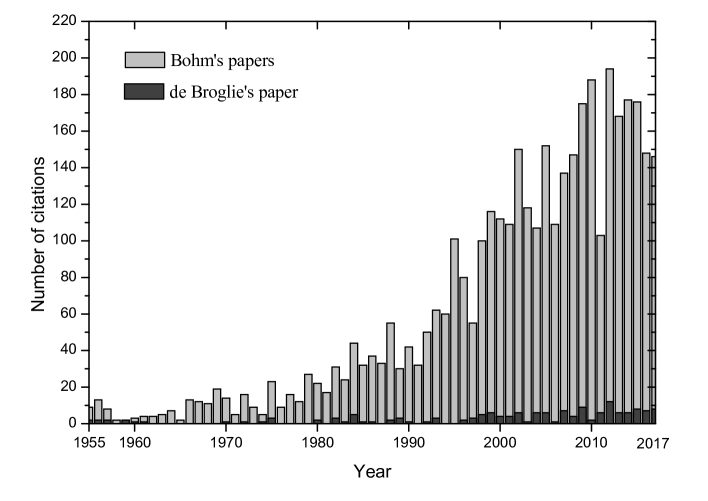
Figure 1: Number of citations per year for (a) the two 1952 David Bohm’s papers entitled “A suggested interpretation of the quantum theory in terms of hidden variables” om.bohm1952a ; om.bohm1952b and (b) Louis de Broglie’s paper “La mécanique ondulatorie et la structure atomique de la matière et du rayonnement”  om.debroglie1927b . Data retreived from ISI Web of Knowledge om.isiweb in December 2017.

III.4 On the book contents

The book contains ten chapters. The first chapter provides an accessible introduction to Bohmian mechanics. The rest of chapters present practical examples on the applicability of Bohmian mechanics. Let us start mentioning the cover of this second edition of the book. It represents the wave and particle nature of electrons according to the Bohmian theory. In particular, we see the Bohmian trajectories of an electron which suffers Klein tunneling when impinging on a triangular potential barrier of a graphene structure. The wave packet of the electron corresponding to the bispinor solution of the Dirac equation (electron with positive and negative energies) is also plotted.

Chapter one is the longest one and it is entitled Overview of Bohmian mechanics. It is written by Xavier Oriols and Jordi Mompart, the editors of the book, both from the Universitat Autònoma de Barcelona, Spain. This chapter is intended to be an introduction to any newcomer interested in Bohmian mechanics. Only basic concepts of classical and quantum mechanics are assumed. The chapter is divided into four different sections. First, the historical development of Bohmian mechanics is explained. Then, Bohmian mechanics for single particle and for many particle systems (with spin and entanglement discussions) are presented. Finally, the topic of Bohmian measurement is addressed in section four. The chapter contains also a list of solved problems and easily implementable codes for computation of Bohmian trajectories.

Chapter two is entitled Hydrogen photoionization with strong lasers. It is written by Albert Benseny from the Okinawa Institute of Science and Technology in Japan; Antonio Picón and Luis Plaja from the Universidad de Salamanca, Spain; Jordi Mompart from the Universitat Autònoma de Barcelona, Spain and Luis Roso from the CLPU, the Laser Center for Ultrashort and Ultraintense Pulses, in Salamanca. They discuss the dynamics of a single hydrogen atom interacting with a strong laser. In particular, the Bohmian trajectories of these electrons represent an interesting illustrating view, with new calculation methods (i.e., Bohmian computing), of both the above threshold ionization and the harmonic generation spectra problems. They do also present a full three dimensional model to discuss the dynamics of Bohmian trajectories when the light beam and the hydrogen atom exchange angular momentum. The chapter does also provide a practical example on how Bohmian mechanics is computed, with an analytical (i.e., Bohmian explaining) procedure, when full (scalar and vector potentials) electromagnetic fields are considered.

The title of chapter three is Atomtronics: Coherent control of atomic flow via adiabatic passage and it is written by Albert Benseny from the Okinawa Institute of Science and Technology in Japan; Joan Bagudà, Xavier Oriols, and Jordi Mompart from the Universitat Autònoma de Barcelona, Spain; and Gerhard Birkl from the Institut für Angewandte Physik, from the Technische Universität Darmstadt in Germany. Here, it is discussed an efficient and robust technique to coherently transport a single neutral atom, a single hole, or even a Bose–Einstein condensate between the two extreme traps of the triple-well potential. The dynamical evolution of this system with the direct integration of the Schrödinger equation presents a very counterintuitive effect: by slowing down the total time duration of the transport process it is possible to achieve atomic transport between the two extrem traps with a very small (almost negligible) probability to populate the middle trap. The analytical (i.e., Bohmian explaining) solution of this problem with Bohmian trajectories enlightens the role of the particle conservation law in quantum systems showing that the negligible particle presence is due to a sudden particle acceleration yielding, in fact, ultra-high atomic velocities. The Bohmian contribution opens the discussion about the possible detection of these high velocities or the need for a relativistic formulation to accurately describe such a simple quantum system.

Chapter four, entitled Bohmian pathways into Chemistry: A brief overview, is prepared by Ángel S. Sanz, from the Universidad Complutense de Madrid, Spain, and deals with the issue of how the Bohmian computing abilities have been explored and exploited in Chemistry over decades. Interestingly, contrary to Physics, Bohmian mechanics has always found a better accommodation and acceptance within different areas of Chemistry, where the pedagogical advantages mentioned by John Bell have been widely recognized. Because providing an exhaustive account on the applications (both as a problem solver and as a computational tool) where Bohmian mechanics has been of relevance within Chemistry would exceed the scope of the chapter, it has been prepared in a way that may serve the reader as a guide to acquire a general perspective (or impression) on how this trajectory-based quantum approach has permeated the different traditional levels or pathways to approach the problems of interest in Chemistry.

Chapter five, whose title is Adaptive quantum Monte Carlo approach states for high-dimensional systems, is written by Eric R. Bittner, Donald J. Kouri, Sean Derrickson, from the University of Houston; and Jeremy B. Maddox, from the Western Kentucky University, in USA. They provide one particular example on the success of Bohmian mechanics in the chemistry community. In this chapter, the authors explain their Bohmian computing development for knowing the ab initio quantum mechanical structure, energetics and thermodynamics of multi-atoms systems. They use a variational approach that finds the quantum ground sate (or even excited states at finite temperature) using a statistical modeling approach for determining the best estimate of a quantum potential for a multi-dimensional system.

Chapter six is entitled Nanoelectronics: Quantum electron transport. It is written by Enrique Colomés, Devashish Pandey, Alfonso Alarcón and Xavier Oriols from the Universitat Autònoma de Barcelona, Spain; Zhen Zhan from the Wuhan University, in China; Guillem Albareda from Max Planck Institute for the Structure and Dynamics of Matter in Germany and Fabio Lorenzo Traversa from University of California, in USA. The authors explain the ability of their own many-particle Bohmian computing algorithm to understand and model nanoscale electron devices. In particular, it is shown that the adaptation of Bohmian mechanics to electron transport in open systems (with interchange of particles and energies) leads to a quantum Monte Carlo algorithm, where randomness appears because of the uncertainties in the number of electrons, their energies and the initial positions of (Bohmian) trajectories. A general, versatile and time-dependent 3D electron transport simulator for nanoelectronic devices, named BITLLES (Bohmian Interacting Transport in Electronic Structures), is presented showing its ability for a full prediction (DC, AC, fluctuations) of the electrical characteristics of any nanoelectronic device. The BITLLES simulator is also applied to graphene structures (by solving the Dirac equation) as reflected in the cover of this book.

Chapter seven, entitled Beyond the eikonal approximation in classical optics and quantum physics, is written by Adriano Orefice, Raffaele Giovanelli and Domenico Ditto from the Università degli Studi di Milano, Italy. It is devoted to discuss how Bohmian thinking can also help in optics, exploring the fact that the time-independent Schrödinger equation is strictly analogous to the Helmholtz equation appearing in classical wave theory. Starting from this equation they obtain indeed, without any omission or approximation, a Hamiltonian set of ray-tracing equations providing (in stationary media) the exact description in term of rays of a family of wave phenomena (such as diffraction and interference) much wider than that allowed by standard geometrical optics, which is contained as a simple limiting case. They show in particular that classical ray trajectories are ruled by a wave potential presenting the same mathematical structure and physical role of Bohm’s quantum potential, and that the same equations of motion obtained for classical rays hold, in suitable dimensionless form, for quantum particle dynamics, leading to analogous trajectories and reducing to classical dynamics in the absence of such a potential.

Chapter eight, entitled Relativistic quantum mechanics and quantum field theory, is written by Hrvoje Nikolić from the Rudjer Bošković Institute, Croatia. This chapter presents a clear example on how a Bohmian thinking on superluminal velocities and nonlocal interactions helps in extending the quantum theory towards relativity and quantum field theory. A relativistic-covariant formulation of relativistic quantum mechanics of fixed number of particles (with or without spin) is presented, based on many-time wavefunctions and on an interpretation of probabilities in the spacetime. These results are used to formulate the Bohmian interpretation of relativistic quantum mechanics in a manifestly relativistic covariant form and are also generalized to quantum field theory. The corresponding Bohmian interpretation of quantum field theory describes an infinite number of particle trajectories. Even though the particle trajectories are continuous, the appearance of creation and destruction of a finite number of particles results from quantum theory of measurements describing entanglement with particle detectors.

Chapter nine, whose title is Sub-quantum accelerating universe, is written by Pedro F. González-Díaz from the Instituto de Física Fundamental, Consejo Superior de Investigaciones Científicas, Spain and and Alberto Rozas-Fernández from the Instituto de Astrofísica e Ciências do Espaço, in Portugal. Contrarily to the general belief, quantum mechanics does not only govern microscopic systems, but it has influence also on the cosmological domain. However, the extension of the Copenhagen version of quantum mechanics to cosmology is not free from conceptual difficulties: the probabilistic interpretation of the wavefunction of the whole universe is somehow misleading because we cannot make statistical “measurements” of different realizations of our universe. This chapter deals with two new cosmological models describing the accelerating universe in the spatially flat case. Also in this chapter there is a discussion on the quantum cosmic models that result from the existence of a nonzero entropy of entanglement. In such a realm, they obtain new cosmic solutions for any arbitrary number of spatial dimensions, studying the stability of these solutions, as well as the emergence of gravitational waves in the realm of the most general models.

Finally, chapter ten entitled Bohmian quantum gravity and cosmology, is written by Nelson Pinto-Neto from the Centro Brasileiro de Pesquisas Físicas, in Brazil, and by Ward Struyve from the Ludwig-Maximilians-Universität München, in Germany. This chapter is another enlightening example on the utility of Bohmian thinking concerning the nature of space-time and mass in physical theories. The authors discuss how many conceptual problems that appear in a description of gravity in quantum mechanical terms, such as the measurement problem and the problem of time, can be overcome by adopting a Bohmian perspective. In addition to solving conceptual problems, the authors show that Bohmian computing in quantum cosmology gives new types of semi-classical approximations to quantum gravity, and approximations for quantum perturbations moving in a quantum background.

IV Historical Development of Bohmian Mechanics

In general, the history of quantum mechanics is explained in textbooks as a chronicle where each step follows naturally from the preceding one. However, it was exactly the opposite. The development of quantum mechanics was a zigzagging route full of misunderstandings and personal disputes. It was a painful history, where scientists were forced to abandon well-established classical concepts and to explore new and imaginative routes. Most of the new routes went nowhere. Others were simply abandoned. Some of the explored routes were successful in providing new mathematical formalisms capable of predicting experiments at the atomic scale. Even such successful routes were painful enough, so relevant scientists, such as Albert Einstein or Erwin Schrödinger, decided not to support them. In this section we will briefly explain the history of one of these routes: Bohmian mechanics. It was first proposed by Louis de Broglie om.debroglie1923 , who abandoned it soon afterward, and rediscovered by David Bohm om.bohm1952a ; om.bohm1952b many years later, and it has been ignored by most of the scientific community since then. We will discuss the historical development of Bohmian mechanics to understand its present status. Also, we will introduce the basic mathematical aspects of the theory, while the formal and rigorous structure will be presented in the subsequent sections.

IV.1 Particles and waves

The quantum theory revolves around the notions of particles and waves. In classical physics, the concept of a particle is very useful for the description of many natural phenomena. A particle is directly related to a trajectory $\vec{r}_{i}[t]$ that defines its position as a continuous function of time, usually found as a solution of a set of differential equations. For example, the planets can be considered particles orbiting around the sun, whose orbits are determined by the classical Newton gravitational laws.

In classical mechanics, it is natural to think that the total number of particles (e.g., planets in the solar system) is conserved, and the particle trajectories must be continuous in time: if a particle goes from one place to another, then, it has to go through all the trajectory positions between these two places. This condition can be summarized with a local conservation law:

$$\frac{\partial\rho(\vec{r},t)}{\partial t}+\vec{\nabla}\vec{j}(\vec{r},t)=0$$ (1)

where $\rho(\vec{r},t)$ is the density of particles and $\vec{j}(\vec{r},t)$ is the particle current density. For an ensemble of point particles at positions $\vec{r}_{i}[t]$ with velocites $\vec{v}_{i}[t]$, it follows that $\rho(\vec{r},t)=\sum\delta(\vec{r}-\vec{r}_{i}[t])$ and $\vec{j}(\vec{r},t)=\sum\vec{v}_{i}[t]\delta(\vec{r}-\vec{r}_{i}[t])$, with $\delta(\vec{r})$ being the Dirac delta function, satisfying Eq. (1). We have used the property that ${\partial\delta(\vec{r}-\vec{r}_{i}[t])}/{\partial t}=-\vec{\nabla}\delta(\vec{r}-\vec{r}_{i}[t]){d\vec{r}_{i}[t]}/{dt}$.

However, the total number of planets in the solar system could be conserved in another (quite different) way. A phenomenon where a planet disappearing (instantaneously) from its orbit and appearing (instantaneously) at another point far away from its original location would certainly conserve the number of planets but it would violate Eq. (1). We must then think of Eq. (1) as a law for the local conservation of particles.

Fields, and particularly waves, also appear in many explanations of physical phenomena. The concept of a field was initially introduced to deal with the interaction of distant particles. For example, there is an interaction between the electrons in an emitting radio antenna at the top of a mountain and those in the receiving antenna at home. Such interaction can be explained through the use of an electromagnetic field. Electrons in the transmitter generate an electromagnetic field, a radio wave, that propagates through the atmosphere and arrives at our antenna, affecting its electrons. Finally, a loudspeaker transforms the electron motion into music at home.

The simplest example of a wave is the so-called plane wave:

$$\psi(\vec{r},t)=e^{i(\omega t-\vec{k}\cdot\vec{r})}$$ (2)

where the angular frequency $\omega$ and the wave vector $\vec{k}$ refer respectively to its temporal and spatial behavior. In particular, the angular frequency $\omega$ specifies when the temporal behavior of such wave is repeated. The value of $\psi(\vec{r_{1}},t_{1})$ at position $\vec{r_{1}}$ and time $t_{1}$ is identical to $\psi(\vec{r_{1}},t_{2})$ when $t_{2}=t_{1}+2\pi n/\omega$ for $n$ integer. The angular frequency $\omega$ can be related to the linear frequency $\nu$ as $\omega=2\pi\nu$. Analogously, the wave vector $\vec{k}$ determines the spatial repetition of the wave, that is, the wavelength $\lambda$. The value of $\psi(\vec{r_{1}},t_{1})$ at position $\vec{r_{1}}$ and time $t_{1}$ is identical to $\psi(\vec{r_{2}},t_{1})$ when $\vec{k}\cdot\vec{r_{2}}=\vec{k}\cdot\vec{r_{1}}+2\pi n$ with $n$ integer. Unlike a trajectory, a wave is defined at all possible positions and times. Waves can be a scalar or a vectorial function and take real or complex values. For example, Eq. (2) is a scalar complex wave of unit amplitude. The waves’ dynamical evolution is determined by a set of differential equations. In our broadcasting example, Maxwell equations define the electromagnetic field of the emitted radio wave that is given by two vectorial functions, one for the electric field and one for the magnetic field.

Whenever the differential equations that govern the fields are linear, one can apply the superposition principle to explain what happens when two or more fields (waves) traverse simultaneously the same region. The modulus of the total field at each position is related to the amplitudes of the individual waves. In some cases, the modulus of the sum of the amplitudes is much smaller than the sum of the modulus of the amplitudes; this is called destructive interference. In other cases, it is roughly equal to the sum of the modulus of the amplitudes; this is called constructive interference.

IV.2 Origins of the quantum theory

At the end of the nineteenth century, Sir Joseph John Thomson discovered the electron, and in 1911, Ernest Rutherford, a New Zealander student working in Thomson’s laboratory, provided experimental evidence that inside atoms, electrons orbited around a nucleus in a similar manner as planets do around the sun. Rutherford’s model of the atom was clearly in contradiction with well-established theories, since classical electromagnetism predicted that orbiting electrons should radiate, gradually lose energy, and spiral inward. Something was missing in the previous explanations, since it seemed that the electron behavior inside an atom could not be explained in terms of classical trajectories. Therefore, alternative ideas needed to be explored to understand atom stability.

In addition, at that time, classical electromagnetism was unable to explain the radiated spectrum of a black body, which is an idealized object that emits a temperature-dependent spectrum of light (like a big fire with different colors, depending on the flame temperature). The predicted continuous intensity spectrum of this radiation became unlimitedly large in the limit of large frequencies, resulting in an unrealistic emission of infinite power, which was called the ultraviolet catastrophe. However, the measured radiation of a black body did not behave in this way, indicating that a wave description of the electromagnetic field was also incomplete.

In summary, at the beginning of the twentieth century, it was clear that natural phenomena such as atom stability or black-body radiation, were not well explained in terms of a particle or a wave description alone. It seemed necessary to merge both concepts.

In 1900, Max Planck suggested om.Planck-BlackBody that black bodies emit and absorb electromagnetic radiation in discrete energies $h\nu$, where $\nu$ is the frequency of the emitted radiation and $h$ is the (now-called) Planck constant. Five years later, Einstein used this discovery in his explanation of the photoelectric effect om.Einstein-Photoelectric , suggesting that light itself was composed of light quanta or photons of energy $h\nu$. Even though this theory solved the black-body radiation problem, the fact that the absorption and emission of light by atoms are discontinuous was still in conflict with the classical description of the light-matter interaction.

In 1913, Niels Bohr om.bohr ; om.bohr2 ; om.bohr3 wrote a revolutionary paper on the hydrogen atom, where he solved the (erroneously predicted in classical terms) instability by postulating that electrons can only orbit around atoms in some particular nonradiating orbits. Thus, atom radiation occurs only when electrons jump from one orbit to another of lower energy. His imaginative postulates were in full agreement with the experiments on spectral lines. Later, in 1924, de Broglie proposed in his PhD dissertation that all particles (such as electrons) exhibit wave-like phenomena like interference or diffraction om.debroglie1923 . In particular, one way to arrive at Bohr’s hypothesis is to think that the electron orbiting around the proton is a stationary wave. Since we know that the probability of finding the electron far from the proton is zero, we can impose such spatial boundary conditions on the shape of such a stationary wave. We will obtain that only very particular shapes of the waves (associated to very particular energies) are allowed. Physics at the atomic scale started to be understandable by mixing the concepts of particles and waves. All these advances were later known as the old quantum theory. The word quantum referred to the minimum unit of any physical entity (e.g., the energy) involved in the interactions at such atomistic scales.

IV.3 “Wave or particle?” vs. “wave and particle”

In the mid-1920s, theoreticians found themselves in a difficult situation when attempting to advance Bohr’s ideas. A group of atomic theoreticians centered on Bohr, Max Born, Wolfgang Pauli, and Werner Heisenberg suspected that the problem went back to trying to understand electron trajectories within atoms. In under two years, a series of unexpected discoveries brought about a scientific revolution om.waerden .

Heisenberg wrote his first paper on quantum mechanics in 1925 om.Heisenber1925 and two years later stated his uncertainty principle om.Heisenber1927 . It was him, with the help of Born and Pascual Jordan, who developed the first version of quantum mechanics based on a matrix formulation om.Born1926 ; om.Heisenber1925 ; om.Heisenber1925b ; om.Heisenber1925c .

In 1926, Schrödinger published An Undulatory Theory of the Mechanics of Atoms and Molecules om.scho1926 , where, inspired by de Broglie’s work om.dB_AnnPhys ; om.debroglie1923 ; om.debroglie1927b , he described material points (such as electrons or protons) in terms of a wave solution of the following (wave) equation:

$$i\hbar\frac{\partial\psi(\vec{r},t)}{\partial t}=-\frac{\hbar^{2}}{2m}\nabla^{2}\psi(\vec{r},t)+V(\vec{r},t)\psi(\vec{r},t)$$ (3)

where $V(\vec{r},t)$ is the potential energy felt by the electron, and the wave (field) $\psi(\vec{r},t)$ was called the wave function. Schrödinger, at first, interpreted his wave function as a description of the electron charge density $q\left|\psi(\vec{r},t)\right|^{2}$ with $q$ the electron charge. Later, Born refined the interpretation of Schrödinger and defined $|\psi(\vec{r},t)|^{2}$ as the probability density of finding the electron in a particular position $\vec{r}$ at time $t$ om.waerden .

Schrödinger’s wave version of quantum mechanics and Heisenberg’s matrix mechanics were apparently incompatible, but they were eventually shown to be equivalent by Wolfgang Ernst Pauli and Carl Eckart, independently om.waerden ; om.waerden2 .

In order to explain the physics behind quantum systems, the concepts of waves and particles should be merged in some way. Two different routes appeared:

1. Wave or particle? The concept of a trajectory was, consciously or unconsciously, abandoned by most of the young scientists (Heisenberg, Pauli, Dirac, Jordan$,\ldots).$ They started a new route, the wave or particle? route, where depending on the experimental situation, one has to choose between a wave or a particle behavior. Electrons are associated basically to probability (amplitude) waves. The particle nature of the electron appears when we measure the position of the electron. In Bohr’s words, an object cannot be both a wave and a particle at the same time; it must be either one or the other, depending upon the situation. This approach, mainly supported by Bohr, is one of the pillars of the Copenhagen, or orthodox, interpretation of quantum mechanics.

2. Wave and particle: Louis de Broglie, on the other hand, presented an explanation of quantum phenomena where the wave and particle concepts merge at the atomic scale, by assuming that a pilot-wave solution of Eq. (3) guides the electron trajectory. This is what we call the Bohmian route. One object cannot be a wave and a particle at the same time, but two can.

The differences between the two routes can be easily seen in the interpretation of the double-slit experiment. A beam of electrons with low intensity (so that electrons are injected one by one) impinges upon an opaque surface with two slits removed on it. A detector screen, on the other side of the surface, detects the position of electrons. Even though the detector screen responds to particles, the pattern of detected particles shows the interference fringes characteristic of waves. The system exhibits, thus, the behavior of both waves (interference patterns) and particles (dots on the screen).

According to the wave or particle? route, first the electron presents a wavelike nature alone when the wave function (whose squared modulus gives the probability density of finding a particle when a position measurement is done) travels through both slits. Suddenly, the wave function collapses into a delta function at a (random) particular position on the screen. The particle-like nature of the electron appears, while its wavelike nature disappears. Since the screen positions where collapses occur follow the probability distribution dictated by the squared modulus of the wave function, a wave interference pattern appears on the detector screen.

According to the wave and particle route, the wave function (whose squared modulus means the particle probability density of being at a certain position, regardless of the measurement process) travels through both slits. At the same time, a well-defined trajectory is associated with the electron. Such a trajectory passes through only one of the slits. The final position of the particle on the detector screen and the slit through which the particle passes is determined by the initial position of the particle. Such an initial position is not controllable by the experimentalist, so there is an appearance of randomness in the pattern of detection. The wave function guides the particles in such a way that they avoid those regions in which the interference is destructive and are attracted to the regions in which the interference is constructive, giving rise to the interference pattern on the detector screen. Let us quote the enlightening summary of Bell om.Bell1987 :

Is it not clear from the smallness of the scintillation on the screen that we have to do with a particle? And is it not clear, from the diffraction and interference patterns, that the motion of the particle is directed by a wave? De Broglie showed in detail how the motion of a particle, passing through just one of two holes in screen, could be influenced by waves propagating through both holes. And so influenced that the particle does not go where the waves cancel out, but is attracted to where they cooperate. This idea seems to me so natural and simple, to resolve the wave-particle dilemma in such a clear and ordinary way, that it is a great mystery to me that it was so generally ignored.

Now, with almost a century of perspective and the knowledge that both routes give exactly the same experimental predictions, it seems that such great scientists took the strangest route. Let us imagine that a student asks his or her professor, “What is an electron?” The answer of a (Copenhagen) professor could be, “The electron is not a wave nor a particle. But, do not worry! You do not have to know what an electron is to (compute observable results) pass the exam.” If the student insists, the professor might reply, “Shut up and calculate.”

Another example of the vagueness of the orthodox formulation can be illustrated by the question that Einstein posed to Abraham Pais: “Do you really think the moon is not there if you are not looking at it?” The answer of a Copenhagen professor, such as Bohr, would be, “I do not need to answer such a question, because you cannot ask me such question experimentally”. This answer is technically correct because, from an orthodox point of view, the property of the position of an object is undefined unless we measure it. But, knowing now that an explanation of quantum phenomena can be formulated with well defined positions of particles independently of being measured or not, the previous answer seems a bit impertinent.

On the other hand, an alternative (Bohmian) professor would answer, “Electrons are particles whose trajectories are guided by a pilot field which is the wave function solution of the Schrödinger equation. There is some uncertainty in the initial conditions of the trajectories, so that experiments have also some uncertainties.” With such a simple explanation, the student would understand perfectly the role of the wave and the particle in the description of quantum phenomena. Furthermore, in the Bohmian interpretation, the position of an electron (or the moon) while we are not looking at it, is always defined, even though it is a hidden variable for experimentalists.

One of the reasons that led the proponents of quantum mechanics to choose the wave or particle? route is that the predictions about the positions of electrons are uncertain because the wave function is spread out over a volume. This effect is known as the uncertainty principle: it is not possible to measure, simultaneously, the exact position and velocity (momentum) of a particle. Therefore, scientists preferred to look for an explanation of quantum effects without the concept of a trajectory that seemed unmeasurable. They constructed a theory to explain the quantum world where the concept of trajectory was not present in the ontology. However, their argumentation to neglect the use of trajectories is, somehow, unfair and unjustified, since it relies on the “principle” that the ontology of a physical theory should not contain entities that cannot be observed.

In addition, everyone with experience on Fourier transforms of conjugate variables recognizes the quantum uncertainty principle as a trivial effect present in any wave theory where the momentum of a particle depends on the slope of its associated wave function. Then, a very localized particle would have a very sharp wave function. In this case such a wave function would have a great slope that implies a large range of possible momenta. On the contrary, if the wave function is built from a quite small range of momenta, then it will have a large spatial dispersion.

IV.4 Louis de Broglie and the fifth Solvay Conference

Perhaps the most relevant event for the development of the quantum theory was the fifth Solvay Conference, which took place from October 24–29, 1927, in Brussels om.valentini2009Solvay . As on previous occasions, the participants stayed at Hôtel Britannique, invited by Ernest Solvay, a Belgian chemist and industrialist with philanthropic purposes due to the exploitation of his numerous patents. There, de Broglie presented his recently developed pilot wave theory and how it could account for quantum interference phenomena with electrons om.valentini2009Solvay . He did not receive an enthusiastic reaction from the illustrious audience gathered for the occasion. In the following months, it seems that he had some difficulties in interpreting quantum measurement with his theory and decided to avoid his new pilot wave theory. In fact, one (nonscientific) reason that perhaps forced de Broglie to give up on his theory was that he worked isolated, having little contact with the main research centers in Berlin, Copenhagen, Cambridge, or Munich. By contrast, most of the Copenhagen contributors worked with fluid and constant collaborations among them.

Finally, let us mention that the elements of the pilot wave theory (electrons guided by waves) were already in place in de Broglie’s thesis in 1924 om.debroglie1923 , before either matrix or wave mechanics existed. In fact, Schrödinger used the de Broglie phases to develop his famous equation (see Eq. (3)). In addition, it is important to remark that de Broglie himself developed a single-particle and a many-particle description of his pilot waves, visualizing also the nonlocality of the latter om.valentini2009Solvay . Perhaps, his remarkable contribution and influence have not been fairly recognized by scientists and historians because he abandoned his own ideas rapidly without properly defending them om.valentini2009Solvay ; om.Broglie1956 .

IV.5 Albert Einstein and locality

Not even Einstein gave explicit support to the pilot wave theory om.waerden . It remains almost unknown that in 1927, the same year that de Broglie published his pilot wave theory om.debroglie1927b , Einstein worked out an alternative version of the pilot wave with trajectories determined by many-particle wave functions. However, before the paper appeared in print, Einstein phoned the editor to withdraw it. The paper remains unpublished, but its contents are known from a manuscript om.einsteinhidden1927 ; om.Hollaneinstein .

It seems that Einstein, who was unsatisfied with the Copenhagen approach, did not like the pilot wave approach either because both interpretations have this notion of action at a distance: particles that are far away from each other can profoundly and instantaneously affect each other. As the father of the theory of relativity, he believed that action at a distance cannot travel faster than the speed of light. Let Bohm explain the difficulties of Einstein with both the Bohmian and the orthodox interpretations om.Bohminterview :

In the fifties, I sent [my Quantum Theory book] around to various quantum physicists - including Niels Bohr, Albert Einstein, and Wolfgang Pauli. Bohr didn’t answer, but Pauli liked it. Albert Einstein sent me a message that he’d like to talk with me. When we met he said the book had done about as well as you could do with quantum mechanics. But he was still not convinced it was a satisfactory theory. Einstein’s objection was not merely that it was statistical. He felt it was a kind of abstraction; quantum mechanics got correct results but left out much that would have made it intelligible. I came up with the causal interpretation (that the electron is a particle, but it also has a field around it. The particle is never separated from that field, and the field affects the movement of the particle in certain ways). Einstein didn’t like it, though, because the interpretation had this notion of action at a distance: Things that are far away from each other profoundly affect each other. He believed only in local action.

Einstein, together with Boris Podolsky and Nathan Rosen, presented objections to the orthodox quantum theory in the famous EPR article in 1935, entitled “Can Quantum-Mechanical Description of Physical Reality Be Considered Complete?” om.Einstein_rosen1935 . There, they argued that on the basis of the absence of action at a distance, quantum theory must be incomplete. In other words, quantum theory is either nonlocal or incomplete. Einstein believed that locality was a fundamental principle of physics, so he adhered to the view that quantum theory was incomplete. Einstein died in 1955, convinced that a correct reformulation of quantum theory would preserve local causality. We will see later that he was wrong in this particular point.

IV.6 David Bohm and why the “impossibility proofs” were wrong?

Perhaps the first utility of Bohm’s work was the demonstration that the mentioned von Neumann theorem about the “impossible proofs” had limited validity. In 1932, von Neumann put quantum theory on a firm theoretical basis om.impossibility_proofs . Some of the earlier works lacked mathematical rigor, and he put the entire theory into the setting of operator algebra. In particular, von Neumann studied the following question: “If the present mathematical formulation of the quantum theory and its usual probability interpretation are assumed to lead to absolutely correct results for every experiment that can ever be done, can quantum-mechanical probabilities be understood in terms of any conceivable distribution over hidden parameters?” von Neumann answered this question negatively. His conclusions, however, relied on the fact that he implicitly restricted his proof to an excessively narrow class of hidden variables, excluding Bohm’s hidden variables model. In other words, Bohmian mechanics is a counterexample that disproves von Neumann’s conclusions, in the sense that it is possible to obtain the very same predictions of orthodox quantum mechanics with a hidden variables theory om.Holand1993 ; om.Bell1987 .

Bohm’s formulation of quantum mechanics appeared after the orthodox formalism was fully established. Bohm was, perhaps, the first person to genuinely understand the significance and fundamental implications of the description of quantum phenomena with trajectories guided by waves. Ironically, in 1951, Bohm wrote a book, Quantum Theory om.bohmbook , where he provided “proof that quantum theory is inconsistent with hidden variables” (see page 622 in [21]). In fact, he wrote in a footnote in that section, “We do not wish to imply here that anyone has ever produced a concrete and successful example of such a [hidden variables] theory, but only state that such theory is, as far as we know, conceivable.” Furthermore, the book does also contain an unusually long chapter devoted to the quantum theory of the process of measurement, where Bohm discusses how the measurement itself can be described from the time evolution of a many-particle wave function, rather than invoking the wave function collapse. It seems that Bohm became dissatisfied with the orthodox approach that he had written in his book and began to develop his own causal formulation of quantum theory, which he published in 1952 om.bohm1952a ; om.bohm1952b .

The original papers of Bohm in 1952 om.bohm1952a ; om.bohm1952b provide a formal justification of the guidance equation developed 25 years before by de Broglie. Instead of reproducing his exact mathematical development in terms of the quantum Hamilton–Jacobi equation, here, we discuss a very simple explanation of the guidance equation. By a simple mathematical manipulation of the (wave) equation, Eq. (3), we can find the local (particle) continuity equation, Eq. (1), discussed at the beginning of this section. From the standard definition of the current density $\vec{j}(\vec{r},t)$, as a product of the particle density $\rho(\vec{r},t)=|\psi(\vec{r},t)|^{2}$ and the velocity $\vec{v}(\vec{r},t)$, we can exactly obtain the guidance equation that was predicted by de Broglie and Bohm for the particle velocity:

$$\frac{d\vec{r}(t)}{dt}=\vec{v}(\vec{r},t)=\frac{\vec{j}(\vec{r},t)}{\rho(\vec{r},t)}$$ (4)

There was another important point explained by Bohm in 1952. If one considers an ensemble of trajectories whose initial positions at time $t=0$ are distributed according to $\rho(\vec{r},0)=|\psi(\vec{r},0)|^{2}$, such an ensemble of trajectories will reproduce $\rho(\vec{r},t)=|\psi(\vec{r},t)|^{2}$ at any other time if the trajectories follow the guidance equation, Eq. (4). Therefore, we are able to exactly reproduce the time evolution of the wave function solution of Eq. (3) from an ensemble of trajectories guided by waves. Let Bohm himself explain this revolutionary point in the first page of his original reference om.bohm1952a :

The usual [Copenhagen] interpretation of the quantum theory is based on an assumption […] that the physical state of an individual system is completely specified by a wave function that determines only the probabilities of actual results that can be obtained in a statistical ensemble of similar experiments. […] In contrast, this alternative interpretation permits us to conceive of each individual system as being in a precisely definable state, whose changes with time are determined by definite laws, analogous to (but not identical with) the classical equations of motion. Quantum mechanical probabilities are regarded (like their counterpart in classical mechanics) as only a practical necessity and not as a manifestation of an inherent lack of complete determination in the properties of matter at the quantum level.

Bohm’s original papers do also provide a different path to find the trajectories by introducing the polar form of the wave function $\psi(\vec{r},t)=R(\vec{r},t)e^{iS(\vec{r},t)/\hbar}$ into the (nonrelativistic) Schrödinger equation, Eq. (3). Let us emphasize that $R(\vec{r},t)$ and $S(\vec{r},t)$ are real (not complex) functions. Then, after a quite simple manipulation, one obtains from the real part a quantum Hamilton–Jacobi equation:

$$\frac{\partial S(\vec{r},t)}{\partial t}+\frac{1}{2m}\left(\vec{\nabla}S(\vec{r},t)\right)^{2}+V(\vec{r},t)+Q(\vec{r},t)=0$$ (5)

where we have defined the quantum potential $Q(\vec{r},t)$ as:

$$Q(\vec{r},t)=-\frac{\hbar^{2}}{2m}\frac{\vec{\nabla}^{2}R(\vec{r},t)}{R(\vec{r},t)}$$ (6)

which is the only difference with respect to the classical Hamilton–Jacobi equation if the velocity is defined as $\vec{v}=\vec{\nabla}S/m$. Such an alternative explanation provides an additional justification for the guidance equation, Eq. (4) (see problem 6). It allows a second-order interpretation of Bohmian trajectories in terms of acceleration, forces, and energies. In particular, in this second-order point of view, the new quantum potential $Q(\vec{r},t)$ is responsible for the deviations of the Bohmian trajectories from the classical behavior that can be expected from the classical potential $V(\vec{r},t)$. As we will discuss later, the quantum potential of a system of $N$ particles will be the responsible for the (nonclassical) nonlocal causality of Bohmian mechanics.

Bohm completed the work of de Broglie in two fundamental aspects. First, as explained before, he demonstrated that Bohmian mechanics leads to exactly the same predictions as the ones obtained by orthodox quantum mechanics. Second, he provided a theory of measurement. He developed an explanation of the measurement problem without invoking the wave function collapse. The theory of Bohmian measurement will be discussed in Sec. VII. Some authors argue that if we could change history, allowing Bohm to help de Broglie defend his pilot wave theory in the Solvay Conference, Bohmian mechanics would now be certainly taught at universities om.nikolic2008a . The enlightening work of Bohm, however, appeared 25 years too late, once the Copenhagen interpretation of quantum phenomena was already too well established.

After the Solvay Conference, Bohr, Heisenberg, and their colleagues spread the new interpretation around the world and convinced the vast majority of the physics community that the Copenhagen theory worked with extraordinary precision. A lot of young physicists were attracted to European institutes to study with the “fathers” of this new theory, and during the second quarter of the twentieth century, as good disciples, they spread the Copenhagen interpretation over the entire globe. In his 1976 Nobel lecture, Murray Gell-Mann referred to this question: “Niels Bohr brainwashed an entire generation of physicists into believing that the problem [of the interpretation of quantum mechanics] had been solved fifty years ago” om.hard .

Finally, we summarize the importance of Bohm’s work with another magistral quote from Bell that appears in a 1982 paper entitled “On the Impossible Pilot Wave” and collected in his famous book Speakable and Unspeakable in Quantum Mechanics om.Bell1987 :

But in 1952 I saw the impossible done. It was in papers by David Bohm. Bohm showed explicitly how parameters could indeed be introduced, into nonrelativistic wave mechanics, with the help of which the indeterministic description could be transformed into a deterministic one. More importantly, in my opinion, the subjectivity of the “orthodox” version, the necessary reference to the “observer,” could be eliminated. Moreover, the essential idea was on that had been advanced already by de Broglie in 1927, in his “pilot wave” picture. But why then had Born not told me of this “pilot wave”? If only to point out what was wrong with it? Why did von Neumann not consider it? More extraordinarily, why did people go on producing “impossibility” proofs after 1952, and as recently as 1978? When even Pauli, Rosenfeld, and Heisenberg, could produce no more devastating criticism of Bohm’s version than to brand it as “metaphysical” and “ideological”? Why is the pilot wave picture ignored in textbooks? Should it not be taught, not as the only way, but as an antidote to the prevailing complacency? To show that vagueness, subjectivity, and indeterminism, are not forced on us by experimental facts, but by deliberate theoretical choice?

IV.7 John Bell and nonlocality

Along this introduction, we have already mentioned Bell’s positive opinion on Bohmian mechanics. Furthermore, his opinion about the Copenhagen interpretation was that the orthodox theory is “unprofessionally vague and ambiguous” om.Bell1987 ; om.bell1990 ; om.bell1982 ; om.Bell1964 in so far as its fundamental dynamics is expressed in terms of “words which, however, legitime and necessary in application, have no place in a formulation with any pretension to physical precision” om.bell1990 .

Bell spent most of his professional career at the European Organization for Nuclear Research (CERN), working almost exclusively on theoretical particle physics and on accelerator design, but found time to pursue a major avocation investigating the foundations of quantum theory . As seen in many of his quotes used in this introduction, his didactic ability to defend Bohmian mechanics against many unjustified attacks has been of extraordinary importance for maintaining the work of de Broglie and Bohm alive among the scientific community. Fortunately, Bell himself had his own reward from this unbreakable support of Bohmian mechanics. His outstanding work on locality and causality was directly inspired by his deep knowledge of Bohmian mechanics. Bell’s theorem has been called “the most profound discovery of science” om.stapp1977 .

Bell’s most relevant contribution to physics is probably the demonstration that quantum mechanics is nonlocal, contrarily to what Einstein expected. In 1964, inspired by the EPR paper om.Einstein_rosen1935 and Bohm’s work on nonlocal hidden variables, Bell elaborated a theorem establishing clear mathematical inequalities, now known as Bell inequalities, for experimental results that would be fulfilled by local theories but would be violated by nonlocal ones om.Bell1964 . Over the past 30 years, a great number of Bell test experiments have been conducted. These experiments have confirmed that Bell’s inequalities are violated (see, for example, Ref. om.aspect1982 ). Therefore, we have to conclude that quantum experimental results cannot be explained with local hidden variable theories. According to Bell, we must accept the real existence, in nature, of faster-than-light causation.

The experimental violation of Bell’s inequalities gave direct support, not only to the Copenhagen interpretation, but also to Bohm’s formulation of quantum theory, since both are nonlocal theories.

In the Bohmian case, as we have discussed, the quantum potential of $N$ entangled particles is defined in a $3N$ configuration space so that an action on the first particle can have an instantaneous (i.e., faster-than-light) causal effect on the last particle. In Bohmian mechanics, one can understand that the quantum potential is responsible for the instantaneous nonlocal changes on the trajectories of quantum particles. Let Bell explain this point in his own words om.Bell1987 :

That the guiding wave, in the general case, propagates not in ordinary three-dimensional (3D) space but in a multidimensional configuration space is the origin of the notorious “nonlocality” of quantum mechanics. It is a merit of the de Broglie–Bohm version [of quantum mechanics] to bring this out so explicitly that it cannot be ignored.

Unfortunately, as already happened with the von Neumann theorem om.impossibility_proofs , there is an historical misunderstanding about the consequences of Bell’s theorems on Bohmian mechanics. Let us mention just one example that appeared in a prestigious journal in 2000 om.100years :

In the mid-1960s John S. Bell showed that if hidden variables existed, experimentally observed probabilities would have to fall below certain limits, dubbed Bell’s inequalities. Experiments were carried out by a number of groups, which found that the inequalities were violated. Their collective data came down decisively against the possibility of hidden variables.

The author of this sentence has omitted the adjective “local” when he mentions hidden variables. Therefore, a confident reader, who has no time to read Bell’s and Bohm’s works, will understand that Bohmian mechanics is refuted by Bell’s theorem. However, it is exactly the contrary. Bell’s inequalities give direct support to Bohmian mechanics. Unfortunately, this misunderstanding appeared, and continues to appear, in many scientific articles, propagating into textbooks, websites, etc., provoking further comments and replies in the scientific literature. This discussion can give the impression that there still exists some controversy about the validity of Bohmian mechanics for all non-relativistic quantum phenomena or that there is “something unclear” about it, which is clearly not the case.

IV.8 Quantum hydrodynamics

It is sometimes claimed that ideas similar to those developed by de Broglie were put forward by Madelung in 1926 om.Madelung . What Madelung proposed, however, was to regard an electron with mass $m$ and wave function $\psi(\vec{r},t)$ not as a particle with a determined trajectory but as a continuous fluid with mass density $m\left|\psi(\vec{r},t)\right|^{2}$ om.wyatt2005 ; om.Takabayasi . In Madelung’s hydrodynamic interpretation of Eq. (3), the fluid velocity coincides mathematically with de Broglie’s guiding Eq. (4), but the ontological interpretation is quite different.

Let us return again to the double-slit experiment to understand Madelung’s point of view. Orthodox quantum mechanics does not predict what happens to a single electron crossing a double slit, but it predicts what is the statistical probability of detecting electrons when we consider an infinite ensemble of such experiments. In contrast, the proposal from de Broglie and Bohm intends to predict what happens, in principle, to a single electron. At the end of the day, however, because it is not possible to determine the initial position of such a single electron with better uncertainty than that obtained from the initial wave packet spatial dispersion, Bohmian mechanics also provides statistical results. In this regard, Madelung was not interested in dealing with a single-electron trajectory but with the ensemble. When we deal with a very large (infinite) number of particles (trajectories), the particle and current densities that appear in Eq. (1) are no longer discrete functions (sum of deltas) anymore but they have to be interpreted as continuous functions. Aerodynamics and hydrodynamics are examples of such continuous material systems. The concept of an individual trajectory becomes irrelevant in these disciplines but Eq. (1) is still present. In summary, from an ontological point of view, Madelung’s proposal is completely orthodox. However, from a mathematical point of view, its formalism (and computational abilities) is very similar to de Broglie’s proposal. Therefore, a reader who does not feel comfortable with the ideas of Bohm and de Broglie can assume Madelung’s point of view and use many of the concepts explained in this book as a mathematical computational tool.

IV.9 Is Bohmian mechanics a useful theory?

Our historical introduction to Bohmian mechanics ends here. The reader has certainly noticed that we have some preference for the Bohmian interpretation over the Copenhagen, orthodox, explanation of quantum phenomena. Obviously, we have a profound and sincere respect for the Copenhagen interpretation of quantum phenomena and its extraordinary computing capabilities. As discussed in in the section ”What Is a Quantum Theory” in the introduction, a quantum theory connects the ontological and empirical planes. The scientific method is based on experiments. From an empirical point of view, what we have to expect from a physical theory that describes natural phenomena is quite pragmatic. As Bohr said (see page 228 in om.bohr1949 ):

In my opinion, there could be no other way to deem a logically consistent mathematical formalism than by demonstrating the departure of its consequence from experience or by proving that its predictions did not exhaust the possibilities of observations.

Curiously, similar empirical arguments were used by Bohm to defend his causal theory against its many detractors (see page 18 in om.Bohm1953b ):

In conclusion, the author would like to state that we would admit only two valid reasons for discarding a theory that explains a wide range of phenomena. One is that the theory is not internally consistent, and the second is that it disagrees with experiments.

In summary, from all the discussions done up to here, the only statement that we will use in the rest of the book is that one cannot discard an interpretation of quantum phenomena in terms of wave functions and trajectories because it is internally consistent and it agrees with experiments. Once such a statement is accepted, other practical questions about Bohmian mechanics appear naturally, for example, is Bohmian mechanics a useful computational tool for predicting the results of quantum experiments? Although it provides identical predictions as the orthodox formalism, are there advantages in understanding/visualizing/explaining quantum experiments in terms of quantum trajectories? Or, even, is it a recommended formalism for thinking about limits and extensions of (nonrelativistic) quantum theory? This book, through several examples in the following chapters, will try to convince the reader that the answer to these three questions is affirmative.

V Bohmian Mechanics for a Single Particle

After the previous historical introduction, we start with the formal presentation of Bohmian mechanics for a single particle. Usually, new scientific knowledge is built from small variations of old ideas. This explains why the initial development of quantum theory (see Sec. IV.3) was so traumatic. Quantum explanations did not evolve from a small variation of classical mechanics but from radically new ideas. The languages of both theories were completely different. Classical theory provides an explanation of a physical experiment on particles in terms of a well-defined trajectory, while the orthodox quantum theory needs a wave function. Here, we will see that both a wave description of an ensemble of classical particles and a description of quantum systems with trajectories are possible. Starting by setting a common language for both classical and quantum theories will certainly improve our understanding on the similarities and differences between them.

V.1 Preliminary discussions

For a reader without any previous knowledge on quantum mechanics, the following sections would be not only a presentation on Bohmian mechanics, but also on quantum mechanics in general. The Copenhagen and the Bohmian wave functions have exactly the same time evolution (when the same configuration space is used in both cases). In addition, the Bohmian wave function is complemented by a Bohmian trajectory which appears in a natural way when developing a trajectory-based explanation of quantum mechanics as we will discuss in section 1.2.3.

The initial formulation of quantum mechanics with Bohmian trajectories developed by de Broglie and Bohm was perfomed for dynamical systems with associated velocities much slower than the speed of light. Although it is, in principle, possible to extend Bohmian mechanics to relativistic systems (see, for example, chapter 8 and Refs. om.extra6 ; om.extra7 ; om.ward ), we will only deal in this chapter with nonrelativistic systems.

In order to simplify as much as possible our mathematical notation, we will first study a single spinless particle living in a one-dimensional (1D) space. The spatial degree of freedom of the particle will be represented by $x$. The generalization of all the arguments mentioned in this section into a single particle in a 3D space is quite simple. However, the practical solution of a single-particle Schrödinger equation in a 3D space with $x$, $y$ and $z$ degrees of freedom has considerable computational difficulties, as we will discuss in Sec. VI and appendix A.1. In Sec. VI.4 we will consider the role of the spin.

V.2 Creating a wave equation for classical mechanics

In this section we will derive a wave equation similar, although not identical, to the Schrödinger equation for an ensemble of classical trajectories. Certainly, this approach allows us to compare the quantum and classical theories by using a very similar language.

V.2.1 Newton’s second law

Our starting point to derive such a classical wave equation will be Newton’s second law om.Feynmann1963 . Let us consider a particle with mass $m$ in a classical system that moves under the action of a potential $V(x)$, where $x$ is the position coordinate. Here, we assume the potential to be time independent to simplify the mathematical treatment. We define the particle trajectory as $x[t]$ and its velocity as $v[t]=dx[t]/dt\equiv\dot{x}[t]$. Since we are considering a classical system, the trajectory of the particle will be obtained from its acceleration, $a[t]=d^{2}x[t]/dt^{2}\equiv\ddot{x}[t]$, from Newton’s second law:

$$m\ddot{x}[t]=\left[-\frac{\partial V(x)}{\partial x}\right]_{x=x[t]}$$ (7)

Since Eq. (7) is a second-order differential equation, we need to specify both the initial position $x[t_{0}]=x_{0}$ and the initial velocity $v[t_{0}]=v_{0}$ of the particle.

V.2.2 Hamilton’s principle

Apart from Eq. (7), there are other alternative ways to describe a classical system. For example, according to Hamilton’s principle om.Feynmann1963 , the trajectory $x_{\rm p}[t]$ solution of Eq. (7) between two different times, $t_{0}$ and $t_{f}$, provides a stationary value for the action function, $S(x[t];x_{0},t_{0};x_{f},t_{f})$, where $x_{0}=x[t_{0}]$ and $x_{f}=x[t_{f}]$. Hereafter, whenever possible, we will omit the dependence of the action function on $x_{0}$, $t_{0}$, $x_{f}$, and $t_{f}$:

$$\left[\frac{\delta S(x[t])}{\delta x[t]}\right]_{x[t]=x_{\rm p}[t]}=0$$ (8)

where the action function is defined as:

$$S(x[t])=\int_{t_{0}}^{t_{f}}L(x[t],\dot{x}[t])dt$$ (9)

The function $L(x,v)$ is the Lagrangian function:

$$L(x,v)=K(v)-V(x)$$ (10)

with $K(v)=mv^{2}/2$ the kinetic energy of the particle. The Lagrangian equation can also be defined as $L(x,v)=pv-H(x,v)$, where $H(x,p)=K(v)+V(x)$ is the Hamiltonian function and $p=mv$ is the (linear) momentum.

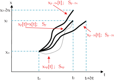
Figure 2: Schematic representation of physical (solid lines) and nonphysical (dotted lines) trajectories in the $(x,t)$ plane. The trajectory $x_{\rm p}[t]$ has the initial time $t_{0}$, the final time $t_{f}$, the initial position $x_{\rm p}[t_{0}]=x_{0}$, and the final position $x_{\rm p}[t_{f}]=x_{f}$. The trajectory $x_{{\rm p}-\delta x}[t]$ is a physical trajectory with identical initial and final conditions as $x_{\rm p}[t]$, except for a different final position $x_{f}+\delta x$. The trajectory $x_{{\rm p}-\delta t}[t]$ is a physical trajectory with identical initial and final conditions as $x_{\rm p}[t]$ but reaching the final point at a larger time $t+\delta t$.

Let us discuss the meaning of a stationary (or extremal) value of the integral in Eq. (9). We denote the physical trajectory solution of Eq. (7) as $x_{\rm p}[t]$ and choose a slightly different trajectory $x_{\rm np}[t]=x_{\rm p}[t]+\delta x[t]$ with the same initial and final conditions, that is, the same $x_{0}$, $t_{0}$, $x_{f}$, and $t_{f}$. Therefore, we have $\delta x[t_{0}]=0$ and $\delta x[t_{f}]=0$. See Fig. 2 for a schematic representation of both trajectories. Equation (8) means that the value of the action function $S_{\rm np}=S(x[t]+\delta x[t];x_{0},t_{0};x_{f},t_{f})$ will always be greater than $S_{\rm p}$; that is, $S_{\rm np}>S_{\rm p}$. Thus, the trajectory that provides a stationary value for the action function is the physical trajectory, $x_{\rm p}[t]$, while $x_{\rm np}[t]=x_{\rm p}[t]+\delta x[t]$ is a nonphysical solution incompatible with Eq. (7).

The numerical evaluation of Eq. (9) to find $S_{\rm p}$ requires the prior knowledge of the trajectory $x_{\rm p}[t]$. If we do not know the trajectory, we would have to evaluate $S(x[t];x_{0},t_{0};x_{f},t_{f})$ for all possible trajectories (starting from $x_{0}$ and $t_{0}$ and ending at $x_{f}$ and $t_{f}$) and choose the one that provides a stationary value. Certainly, it seems that Eq. (8) has little practical utility. However, it provides an interesting starting point to develop our classical wave equation.

V.2.3 Lagrange’s equation

From Hamilton’s principle it is possible to derive the Lagrange’s equation om.Feynmann1963 that gives us the differential equation that the physical trajectory satisfies.

Let us define a trajectory $x_{\rm np}[t]=x_{\rm p}[t]+\delta x[t]$ by adding a small arbitrary displacement $\delta x[t]$ to the physical trajectory. In particular we fix $\delta x[t_{0}]=0$ and $\delta x[t_{f}]=0$, so both trajectories have the same initial and final conditions. A Taylor expansion of the Lagrange function of Eq. (10) around the physical trajectory $x_{\rm p}[t]$ reads:

$$L(x_{\rm np}[t],\dot{x}_{\rm np}[t])=L(x_{\rm p}[t],\dot{x}_{\rm p}[t])+\left[\frac{\partial L}{\partial x}\delta x[t]+\frac{\partial L}{\partial\dot{x}}\dot{\delta x}[t]\right]_{\begin{smallmatrix}x=x_{\rm p}[t]\\ \dot{x}=\dot{x}_{\rm p}[t]\end{smallmatrix}}$$ (11)

The action function of Eq. (9) with the Lagrangian of Eq. (11) gives two contributions. The first term of the right-hand side (r.h.s.) of Eq. (11) is $S_{\rm p}$. After performing an integration by parts on the second part and using $\delta x[t_{0}]=0$ and $\delta x[t_{f}]=0$, we obtain:

$$S(x_{\rm np}[t];x_{0},t_{0};x_{f},t_{f}) = S_{\rm p}+\int_{t_{0}}^{t_{f}}\delta x[t]\times\left(\left[\frac{\partial L}{\partial x}\right]_{\begin{smallmatrix}x=x_{\rm p}[t]\\ \dot{x}=\dot{x}_{\rm p}[t]\end{smallmatrix}}-\frac{d}{dt}\left[\frac{\partial L}{\partial\dot{x}}\right]_{\begin{smallmatrix}x=x_{\rm p}[t]\\ \dot{x}=\dot{x}_{\rm p}[t]\end{smallmatrix}}\right)dt$$

Hamilton’s principle tells us that the action function must take a stationary value for the physical trajectory. This is equivalent to impose that small variations around the physical trajectory do not modify the value of the action, that is, for any (small) variation $\delta x[t]$, $S_{\rm np}=S_{\rm p}$. Thus:

$$\left[\frac{\partial L(x,\dot{x})}{\partial x}\right]_{\begin{smallmatrix}x=x_{\rm p}[t]\\ \dot{x}=\dot{x}_{\rm p}[t]\end{smallmatrix}}-\frac{d}{dt}\left[\frac{\partial L(x,\dot{x})}{\partial\dot{x}}\right]_{\begin{smallmatrix}x=x_{\rm p}[t]\\ \dot{x}=\dot{x}_{\rm p}[t]\end{smallmatrix}}=0$$ (13)

Equation (13) is the Lagrange equation and gives, for a classical system, a differential equation that classical trajectories must fulfill. In order to enlighten the meaning of the Lagrange equation, Eq. (13), we can see that by substituting ${\partial L}/{\partial x}=-{\partial V(x)}/{\partial x}$ and ${\partial L}/{\partial\dot{x}}=mv$ in Eq. (10), we recover:

$$\left[\frac{\partial V(x,t)}{\partial x}\right]_{\begin{smallmatrix}x=x_{\rm p}[t]\\ \dot{x}=\dot{x}_{\rm p}[t]\end{smallmatrix}}-\frac{d}{dt}\left[m\frac{dx[t]}{dt}\right]_{\begin{smallmatrix}x=x_{\rm p}[t]\\ \dot{x}=\dot{x}_{\rm p}[t]\end{smallmatrix}}=0$$ (14)

which is the original Newton’s second law of Eq. (7). In fact, what we have done is to check that Newton’s second law is included in the fundamental Hamilton’s principle.

V.2.4 Equation for an (infinite) ensemble of trajectories

The formalism based on the action function allows us to find not only a single physical trajectory but also the equation for an (infinite) ensemble of physical trajectories with slightly different initial or final conditions. For example, let us define:

$$S_{{\rm p}-\delta t}=S(x_{{\rm p}-\delta t}[t])=\int_{t_{0}}^{t_{f}+\delta t}L(x_{{\rm p}-\delta t}[t],\dot{x}_{{\rm p}-\delta t}[t])dt$$ (15)

$x_{{\rm p}-\delta t}[t]$ being a trajectory with identical initial and final positions as $x_{\rm p}[t]$, but taking a longer time $t_{f}+\delta t$ (see trajectory $x_{{\rm p}-\delta t}[t]$ in Fig. 2). The new physical trajectory $x_{{\rm p}-\delta t}[t]$ can be written as $x_{{\rm p}-\delta t}[t]=x_{\rm p}[t]+\delta x[t]$ for $t\in[t_{0},t_{f}]$. For larger times, $x_{{\rm p}-\delta t}[t_{f}+\delta t]=x_{\rm p}[t_{f}+\delta t]+\delta x[t_{f}+\delta t]$ with $x_{\rm p}[t_{f}+\delta t]=x_{\rm p}[t_{f}]+\dot{x}_{\rm p}[t_{f}]\delta t$, where we have done a first-order Taylor expansion of $x_{\rm p}[t]$ around $t_{f}$ for a small $\delta t$. Since $x_{{\rm p}-\delta t}[t_{f}+\delta t]=x_{\rm p}[t_{f}]$, we obtain:

$$\delta x[t_{f}+\delta t]=-\dot{x}_{\rm p}[t_{f}]\delta t$$ (16)

By following the same steps done after the Taylor expansion in Eq. (11), we obtain:

$$S_{{\rm p}-\delta t} = \int_{t_{0}}^{t_{f}+\delta t}Ldt+\left[\frac{\partial L}{\partial\dot{x}}\delta x[t]\right]_{t_{0}}^{t_{f}+\delta t}+\int_{t_{0}}^{t_{f}+\delta t}\delta x[t]\left(\left[\frac{\partial L}{\partial x}\right]_{x=x[t]}^{\dot{x}=\dot{x}[t]}+\frac{d}{dt}\left[\frac{\partial L}{\partial\dot{x}}\right]_{x=x[t]}^{\dot{x}=\dot{x}[t]}\right)dt\qquad$$ (17)

For the first term of the r.h.s. of Eq. (17), we obtain:

$$\int_{t_{0}}^{t_{f}+\delta t}Ldt=\int_{t_{0}}^{t_{f}}Ldt+\int_{t_{f}}^{t_{f}+\delta t}Ldt=S_{\rm p}+L\delta t$$ (18)

For the second term of the r.h.s. of Eq. (17):

$$\left[\frac{\partial L}{\partial\dot{x}}\delta x[t]\right]_{t_{0}}^{t_{f}+\delta t}=-\left[\frac{\partial L}{\partial\dot{x}}\right]_{x=x[t_{f}+\delta t]}^{\dot{x}=\dot{x}[t_{f}+\delta t]}\dot{x}(t_{f})\delta t=-p[t_{f}+\delta t]\dot{x}[t_{f}]\delta t$$ (19)

where we use Eq. (16), $\delta x[t_{0}]=0$ and ${\partial L}/{\partial\dot{x}}=mv=p$, $p=mv$ being the particle momentum.

Finally, since $x[t]$ is also a physical trajectory that fulfills Lagrange equation, from $t_{0}$ to $t_{f}+\delta t$, we obtain for the third term:

$$\int_{t_{0}}^{t_{f}+\delta t}\delta x[t]\left[\left[\frac{\partial L}{\partial x}\right]_{x=x[t]}^{\dot{x}=\dot{x}[t]}+\frac{d}{dt}\left[\frac{\partial L}{\partial\dot{x}}\right]_{x=x[t]}^{\dot{x}=\dot{x}[t]}\right]dt=0$$ (20)

Putting together Eqs. (18) (19), and (20), we obtain:

$$S_{{\rm p}-\delta t}=S_{\rm p}+L\delta t-p\dot{x}\delta t=S_{\rm p}-H\delta t$$ (21)

So, with ${\partial S}/{\partial t_{f}}=\lim_{\delta t\rightarrow 0}(S_{{\rm p}-\delta t}-S_{\rm p})/\delta t$ we can conclude that:

$$\frac{\partial S(x_{\rm p}[t])}{\partial t_{f}}=-H(x_{\rm p}[t],\dot{x}_{\rm p}[t])$$ (22)

In summary, if $S_{\rm p}$ is the stationary value of the action function for $x_{\rm p}[t]$, then the variation of the new stationary value of another physical trajectory $x_{{\rm p}-\delta t}[t]$, which has identical initial and final conditions but a slightly modified final time, is equal to the Hamiltonian (with a negative sign) evaluated at the final time of the trajectory $x_{\rm p}[t]$. See problem 1 to discuss a particular example.

Next, we will see that the evaluation of the value $S_{{\rm p}-\delta x}$ when we modify the final position $x_{f}+\delta x$ without modifying the initial and final times leads also to an interesting result (see Fig. 2). Notice that the final position of the new physical trajectory $x_{{\rm p}-\delta x}[t]=x[t]+\delta x[t]$ means:

$$\delta x[t_{0}]=0;\;\;\delta x[t_{f}]=\delta x_{f}$$ (23)

By following the same steps done after the Taylor expansion in Eq. (11), we obtain now:

$$S_{{\rm p}-\delta x} = \int_{t_{0}}^{t_{f}}Ldt+\left[\frac{\partial L}{\partial\dot{x}}\delta x[t]\right]_{t_{0}}^{t_{f}}+\int_{t_{0}}^{t_{f}}\delta x[t]\left(\left[\frac{\partial L}{\partial x}\right]_{x=x[t]}^{\dot{x}=\dot{x}[t]}+\frac{d}{dt}\left[\frac{\partial L}{\partial\dot{x}}\right]_{x=x[t]}^{\dot{x}=\dot{x}[t]}\right)dt$$ (24)

The first term of the r.h.s. of Eq. (24) is again $S_{\rm p}$. The second term is

$$\left[\frac{\partial L}{\partial\dot{x}}\delta x[t]\right]_{t_{0}}^{t_{f}}=\left[\frac{\partial L}{\partial\dot{x}}\right]_{x=x[t_{f}]}^{\dot{x}=\dot{x}[t_{f}]}\delta x_{f}=p[t_{f}]\delta x_{f}$$ (25)

where we have used Eq. (23). The third term is zero. We can conclude that ${\partial S}/{\partial x}=\lim_{\delta x\rightarrow 0}(S_{{\rm p}-\delta x}-S_{\rm p})/\delta x$ is equal to:

$$\frac{\partial S(x_{\rm p}[t];x_{0},t_{0};x,t)}{\partial x}=m\dot{x}_{\rm p}[t]=p_{\rm p}[t]$$ (26)

In summary, the variation of the stationary value of the action function when we slightly modify the final position of a physical trajectory is equal to the momentum of the trajectory at the final time. To check Eq. (26) for a particular case, see problem 2.

V.2.5 Classical Hamilton–Jacobi equation

Now, using Eq. (22) and substituting the velocity (momentum) into the Hamiltonian by Eq. (26), we obtain the well-known Hamilton–Jacobi equation:

$$H\left(x,\frac{\partial S(x,t)}{\partial x},t\right)+\frac{\partial S(x,t)}{\partial t}=0$$ (27)

We want to use the Hamilton–Jacobi equation, Eq. (27), to find all the physical trajectories. For this reason, we have eliminated the dependence of $S$ on the trajectory $x[t]$. In addition, we have also eliminated $t_{0}$ and $x_{0}$ because we consider that $x$ and $t$ are not parameters but variables. Notice that Eq. (27) is valid for physical trajectories so that once we know $S(x,t)$, we are able to directly compute all physical trajectories for all possible initial conditions. Therefore, Eq. (27) defines an (infinite) ensemble of trajectories rather than just a single trajectory. However, in most practical cases, the direct solution of the Hamilton–Jacobi equation is much more difficult than using the Newton or Lagrange formulation of classical mechanics. It has limited practical interest. However, it provides a direct theoretical connection with a classical wave equation similar to the Schrödinger equation. See problem 3 for a particular solution of Eq. (27).

V.2.6 Local continuity equation for an (infinite) ensemble of classical particles

Equation (27) can be interesting when dealing with an ensemble of trajectories. For example, it can be used when we have a classical (single-particle) experiment with some practical difficulty in specifying the initial position and velocity of the particle, such that different experimental realizations can have slightly different initial conditions. The ensemble of trajectories solution of Eq. (27) will provide a statistical (probabilistic) description of the classical (single-particle) experiment that accounts for the variability in the initial conditions.

For such an experiment, we can reasonably assume that the variability of the initial position will be limited to a particular spatial region. At the initial time $t_{0}=0$, we can define some distribution of the initial position of the particles $R^{2}(x,0)\geq 0$. Such an ensemble of trajectories will evolve in time according to Eq. (27) so that we will obtain a function $R^{2}(x,t)$ that describes the particular distribution of particles at any time. The function $R^{2}(x,t)$ is constructed by “counting” the number of trajectories present inside the interval $(x,x+dx)$ at time $t$. From Eq. (26), we define the particle velocity as $\dot{x}[t]=(1/m){\partial S(x,t)}/{\partial x}$. Finally, we know that all these classical particles will move, in a continuous way, from one unit of volume to another. Therefore, as we have extensively discussed in Sec. IV.1, we can ensure that the ensemble of trajectories accomplishes the following local conservation law:

$$\frac{\partial R^{2}(x,t)}{\partial t}+\frac{\partial}{\partial x}\left(\frac{1}{m}\frac{\partial S(x,t)}{\partial x}R^{2}(x,t)\right)=0$$ (28)

In summary, Eq. (28) just certifies that if a classical particle goes from one point to another, it has to go through all the trajectory positions between these two places.

V.2.7 Classical wave equation

Now, we have all the ingredients to develop a wave equation for classical mechanics. In previous paragraphs we have been dealing with two (real) functions, $S(x,t)$ and $R(x,t)$. The first, $S(x,t)$, is the action function and appears in the Hamilton–Jacobi equation, Eq. (27). In particular, its spatial derivative determines the velocity of the particles (see Eq. (26)). The second, $R(x,t)$, tells us how an ensemble of trajectories is distributed at each time $t$. It evolves according to the conservation law, Eq. (28). In this sense, we can assume that they are some kind of “field” or “wave” that guide classical particles.

We can construct the following classical (complex) wave function $\psi_{cl}(x,t)=R(x,t)\exp(iS(x,t)/\hbar)$. We divide the action function inside the exponential by $\hbar$ (the reduced Planck’s constant) in order to provide a dimensionless argument. Then, it can be shown that the two previous (real) equations, Eqs. (27) and (28), for $S(x,t)$ and $R(x,t)$ are equivalent to the following (complex) classical wave equation for $\psi_{cl}(x,t)$:

$$i\hbar\frac{\partial\psi_{cl}(x,t)}{\partial t} = -\frac{\hbar^{2}}{2m}\frac{{\partial}^{2}\psi_{cl}(x,t)}{\partial x^{2}}+V(x,t)\psi_{cl}(x,t)+\frac{\hbar^{2}}{2m}\frac{{\partial}^{2}|\psi_{cl}(x,t)|/\partial x^{2}}{|\psi_{cl}(x,t)|}\psi_{cl}(x,t)$$

The demonstration of this expression is left as an exercise to the reader (see problem 4). Additionally, see problem 5 for a solution of the classical wave equation, Eq. (V.2.7), for a free particle.

In conclusion, an ensemble of classical trajectories can be described with a wave function solution of a wave equation. Thus, a common language for classical and quantum mechanics has been obtained by using an (infinite) ensemble of classical trajectories with different initial positions and velocities instead of just one single classical trajectory.

V.3 Trajectories for quantum systems

Before comparing the classical and quantum wave equations, let us first discuss in this section whether trajectories can be also used to describe quantum systems. We will introduce such trajectories in two different ways: first, as a direct consequence of the local conservation of particles extracted from the Schrödinger equation and, second, directly following the work presented by Bohm in his original paper om.bohm1952a .

V.3.1 Schrödinger equation

As discussed in Sec. IV.3, the single-particle Schrödinger equation in a 1D quantum system subjected to a scalar time-dependent potential, $V(x,t)$, is:

$$i\hbar\frac{\partial\psi(x,t)}{\partial t}=-\frac{\hbar^{2}}{2m}\frac{{\partial}^{2}\psi(x,t)}{\partial x^{2}}+V(x,t)\psi(x,t)$$ (30)

It is important to emphasize that in the orthodox interpretation of $\psi(x,t)$, Eq. (30) does not describe a single experiment but an ensemble of identical (single-particle) experiments. The orthodox meaning of the square modulus of the wave function $|\psi(x,t)|^{2}$ is the probability density of finding a particle at position $x$ at time $t$ when a measurement is performed. Such probabilities assume an infinite number of identical experiments.

V.3.2 Local conservation law for an (infinite) ensemble of quantum trajectories

It is known that there is a local continuity equation associated with Eq. (30). Let us first mathematically derive it to later discuss its physical implications.

In order to find a local continuity equation, let us work with $\psi(x,t)$ and its complex conjugate $\psi^{*}(x,t)$. In particular, we can rewrite Eq. (30) as:

$$\psi^{*}(x,t)i\hbar\frac{\partial\psi(x,t)}{\partial t} = -\psi^{*}(x,t)\frac{\hbar^{2}}{2m}\frac{{\partial}^{2}\psi(x,t)}{\partial x^{2}}+\psi^{*}(x,t)V(x,t)\psi(x,t)$$ (31)

and the complex conjugate of Eq. (31) as:

$$-\psi(x,t)i\hbar\frac{\partial\psi^{*}(x,t)}{\partial t} = -\psi(x,t)\frac{\hbar^{2}}{2m}\frac{{\partial}^{2}\psi^{*}(x,t)}{\partial x^{2}}+\psi(x,t)V(x,t)\psi^{*}(x,t)$$ (32)

From Eqs. (31) and (32), we obtain:

$$\frac{\partial|\psi(x,t)|^{2}}{\partial t}=i\frac{\hbar}{2m}\frac{\partial}{\partial x}\left(\psi^{*}(x,t)\frac{{\partial}\psi(x,t)}{\partial x}-\psi(x,t)\frac{{\partial}\psi^{*}(x,t)}{\partial x}\right)$$ (33)

We can easily identify Eq. (33) as the local conservation of particles discussed in Eq. (1) where $\rho(x,t)=|\psi(x,t)|^{2}$ and the current density, $J(x,t)$, is defined as:

$$J(x,t)=i\frac{\hbar}{2m}\left(\psi(x,t)\frac{\partial\psi^{*}(x,t)}{\partial x}-\psi^{*}(x,t)\frac{\partial\psi(x,t)}{\partial x}\right)$$ (34)

Unlike other wave equations, the Schrödinger equation is compatible with a local conservation of particles due to the fact that $V(x,t)$ is a real function. We have noticed above that we can interpret $\rho(x,t)=|\psi(x,t)|^{2}$ as a spatial distribution of an ensemble of trajectories. Each trajectory correspond to a different experiment of the single particle system. Then, in spite of dealing with a single particle system, from a statistical point of view, such (very large) ensemble of trajectories can be interpreted as a (very large) ensemble of particles describing simultaneously all possible experiments. The presence of such local conservation of particles is very relevant for us because it justifies our aim to look for an ensemble of continuous trajectories describing $\rho(x,t)=|\psi(x,t)|^{2}$.

V.3.3 Velocity of Bohmian particles

In Bohmian mechanics, the particle velocity is defined as:

$$v(x,t)=\frac{J(x,t)}{|\psi(x,t)|^{2}}$$ (35)

where $J(x,t)$ is given by Eq. (34). Taking into account that $|\psi(x,t)|^{2}$ is the distribution of the ensemble of particles, it is easy to show that this velocity definition is compatible with the local continuity equation, Eq. (33), and that an ensemble of well-defined trajectories whose initial positions are all selected according to the distribution $|\psi(x,t_{0})|^{2}$ will reproduce $|\psi(x,t)|^{2}$ at all times (see problem 7).

Notice that one could add a divergence-free term to this velocity, and it would still fulfill Eq. (33). Even though this would change the path followed by each individual trajectory, the trajectory distribution and, therefore, the measurement outcomes would remain unchanged. However, if one develops the nonrelativistic limit of a relativistic treatment of Bohmian mechanics, one finds that the divergence-free term does not appear for spin-0-particles and that the velocity is unambiguously defined by Eq. (35). In addition, it has also been demonstrated that possible Bohmian paths are naively observable from a large enough ensemble of weak values om.wiseman2007 ; om.4marian ; om.7colomes giving full support to the definition in Eq. (35). For other values of spin, the situation is a bit more complex om.ward2010 ; om.Holland1999 ; om.Holland2003 and far from the scope of this book.

V.3.4 Quantum Hamilton–Jacobi equation

Following the path described by Bohm in his original paper [2], we will now start from the quantum wave equation, that is, the Schrödinger equation, to arrive at a “quantum” Hamilton–Jacobi equation that describes the motion of quantum trajectories.

The first step is to write the quantum (complex) wave function, $\psi(x,t)=\psi_{r}(x,t)+i\psi_{i}(x,t)$, in polar form:

$$R^{2}(x,t)=\psi_{r}^{2}(x,t)+\psi_{i}^{2}(x,t)$$ (36)

$$S(x,t)=\hbar\arctan\left(\frac{\psi_{i}(x,t)}{\psi_{r}(x,t)}\right)$$ (37)

In principle, $S(x,t)$, the so-called quantum action, is not well defined when $\psi_{r}(x,t)=\psi_{i}(x,t)=0$, that is at those points where $R(x,t)=0$, meaning that no particles will reach them.

The quantum Hamilton–Jacobi equation can be found by introducing $\psi(x,t)=R(x,t)\exp(iS(x,t)/\hbar)$ into Eq. (30). On the one hand, the imaginary part of the resulting equation gives the local conservation law identical to the one shown in Eq. (28), which we rewrite here for convenience:

$$\frac{\partial R^{2}(x,t)}{\partial t}+\frac{\partial}{\partial x}\left(\frac{1}{m}\frac{\partial S(x,t)}{\partial x}R^{2}(x,t)\right)=0$$ (38)

On the other hand, the real part gives a quantum Hamilton–Jacobi equation:

$$\frac{\partial S(x,t)}{\partial t}+\frac{1}{2m}\left(\frac{\partial S(x,t)}{\partial x}\right)^{2}+V(x,t)+Q(x,t)=0$$ (39)

Since the last term in the r.h.s. of the classical wave equation, Eq. (V.2.7), is not present in the Schrödinger equation, Eq. (30), an additional term appears in the quantum Hamilton–Jacobi equation, the so-called quantum potential, defined as:

$$Q(x,t)=-\frac{\hbar^{2}}{2m}\frac{{\partial}^{2}R(x,t)/\partial x^{2}}{R(x,t)}$$ (40)

In conclusion, identical to the classical description of a system obtained from Eq. (39), we obtain an interpretation of the wave function solution of the Schrödinger equation as an ensemble of quantum trajectories with different initial positions and velocities. The velocity of each trajectory $x[t]$ is defined as:

$$v[t]=\left[\frac{1}{m}\frac{\partial S(x,t)}{\partial x}\right]_{x=x[t]}$$ (41)

Interestingly, it can be easily shown that this new expression for the quantum velocity is identical to that mentioned in Eq. (35). See problem 6 to show that both definitions of the velocity of Bohmian trajectories are identical:

$$v(x,t)=\frac{1}{m}\frac{\partial S(x,t)}{\partial x}=\frac{J(x,t)}{|\psi(x,t)|^{2}}$$ (42)

where $J(x,t)$ is defined by Eq. (34).

V.3.5 A quantum Newton-like equation

If we compute the time derivative of the Bohmian velocity defined in Eq. (41), we find a quantum Newton-like equation:

$$m\frac{d}{dt}v(x[t],t)\!=\!m\frac{d}{dt}\left[\frac{1}{m}\frac{\partial S}{\partial x}\right]_{x=x[t]}\!=\!\left[\frac{\partial^{2}S}{\partial x^{2}}\right]_{x=x[t]}\dot{x}[t]+\left[\frac{\partial}{\partial x}\frac{\partial S}{\partial t}\right]_{x=x[t]}$$ (43)

We can rewrite Eq. (43) as:

$$m\frac{d}{dt}v(x[t],t)=\left[\frac{\partial}{\partial x}\left(\frac{1}{2m}\left(\frac{\partial S}{\partial x}\right)^{2}+\frac{\partial S}{\partial t}\right)\right]_{x=x[t]}$$ (44)

Finally, using Eq. (39) we get:

$$m\frac{d}{dt}v(x[t],t)=\left[-\frac{\partial}{\partial x}\left(V(x,t)+Q(x,t)\right)\right]_{x=x[t]}$$ (45)

We conclude here the second route for finding a common language for classical and quantum theories. The quantum (complex) single-particle wave function can be interpreted as an ensemble of trajectories that are all solutions of the same single-particle experiment but with different initial conditions. The quantum trajectories are not solutions of the classical Newton second law with a classical potential but solutions of the quantum Newton second law, Eq. (45), where a quantum potential (that accounts for all nonclassical effects) is added to the classical potential.

V.4 Similarities and differences between classical and quantum mechanics

In previous sections, we have provided a common language for classical and quantum theories, in terms of either wave functions or trajectories, to fairly compare differences and similarities between both theories. Here we emphasize that an attempt to establish similarities and differences between classical and quantum mechanics have to be done by comparing either classical and quantum wave functions or by comparing classical and quantum ensembles of trajectories (not by comparing a single classical trajectory with a quantum wave function). The main difference between the mathematical description of the two theories is that the term $Q(x,t)$ that appears in the quantum Hamilton–Jacobi equation, Eq. (39), is exactly the same term that appears in the classical wave equation, Eq. (V.2.7), but with a change of sign. The term $Q(x,t)$ explains the exotic properties of quantum systems that are missing in their classical counterparts:

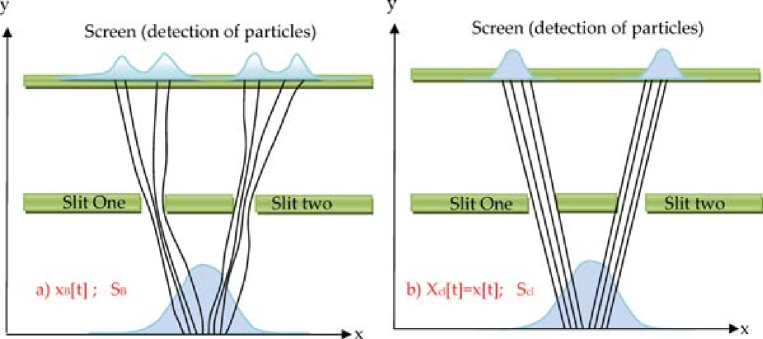
Figure 3: A particle is sent toward a thin plate with two slits cut in it. This single-particle experiment is repeated many times with some uncertainty on the initial conditions of the particle positions. The distribution of detected particles on the screen as a function of the position is different if we deal with a quantum (a) or a classical (b) system. In both cases, we use an identical description of the initial ensemble of particles, that is, identical $R(x,t_{0})$ and $S(x,t_{0})$. However, the classical evolution of the trajectories $x_{cl}[t]$ is described by Eq. (27), which is independent of $R(x,t)$, while quantum (Bohmian) trajectories $x_{B}[t]$ are determined by Eq. (39), which depends explicitly on the other particles of the ensemble through $Q(x,t)$ that depends on $R(x,t)$. These differences can also be understood by observing that the evolution of a classical wave function is described by a nonlinear equation, Eq. (V.2.7), while a quantum wave function evolves with a linear one, Eq. (30).

1. Differences

   1. Quantum superposition
      One can apply the superposition principle to find solutions of the Schrödinger equation, Eq. (30), but it cannot be applied to the classical wave equation, Eq. (V.2.7), since its last term is nonlinear. In fact, if $\psi_{1}(x,t)$ and $\psi_{2}(x,t)$ are solutions of the Schrödinger equation, then $a\psi_{1}(x,t)+b\psi_{2}(x,t)$ with arbitrary complex $a$ and $b$ is also a solution. Quantum mechanics will keep the (complex) amplitudes $a$ and $b$ constant at any time because of its linearity, which is not the case for classical mechanics.

      This is a fundamental difference between classical and quantum systems, which has deep consequences. Quantum mechanics can be developed in a linear vector space, while classical mechanics cannot.

   2. Quantum wholeness
      The presence of $Q(x,t)$ in the quantum Hamilton–Jacobi equation, Eq. (39), implies that Bohmian trajectories depend not only on the classical potential $V(x,t)$ but also on the quantum potential $Q(x,t)$, which is a function of the type of distribution of trajectories associated to different repetitions of the single-particle experiment, $R(x,t)$. In fact, it is the shape and not the absolute value of $R(x,t)$ that acts on each individual quantum trajectory. On the contrary, each classical trajectory can be computed independently of the shape of the ensemble. The fact that the dynamics of one quantum trajectory in one particular experiment depends on the ensemble of other trajectories build from other identical experiments is highly counter-intuitive for our classical mind.

      This surprising result for quantum mechanics can be illustrated with the double-slit experiment om.Dewdney . We assume that the initial wave functions for the classical and quantum ensembles are identical at $t_{0}=0$. Their difference appears in the time evolution of the trajectories. For the quantum trajectories of the ensemble, the shape of the ensemble (whether particles are stopped or not by the double-slit screen) determines the shape of $R(x,t)$, which will affect the dynamics of each trajectory, even those trajectories that are far from the slit (see Fig. 3a). On the contrary, the classical Hamilton–Jacobi equation, Eq. (27), is totally independent of $R(x,t)$, so a single trajectory is completely independent from the rest of trajectories of other experiments as seen in Fig. 3b.

2. Similarities

   1. Uncertainty
      As far as we deal with an ensemble of (classical or quantum) trajectories, there is an uncertainty in the exact value of any magnitude that can be measured from the ensemble. For example, one can compute the mean value and the standard deviation of the position of the classical ensemble. The classical and quantum uncertainties can have different origins, but both ensembles have uncertainties. The classical uncertainty is due to the technical difficulties in exactly repeating the initial conditions of a particular experiments; the quantum uncertainty has a more intrinsic origin om.extra2 ; om.extra9 . See Ref. om.randomness for a discussion on how Bohmian mechanics, although being a deterministic theory at the ontological level, provides a quite simple explanation on the origin of the quantum uncertainty at the empirical level.

      Even assuming their different physical origin, what we want to emphasize here is that it is not licit to compare the uncertainty of a quantum wave function with the uncertainty of a single classical trajectory, saying that the classical trajectory has no uncertainty and the quantum wave function has. As we have previously discussed, we have to compare the uncertainty of classical and quantum wave functions (or classical and quantum ensembles of trajectories).

   2. Initial conditions for the (classical or quantum) Hamilton–Jacobi equation
      The classical Newton equation is a second-order differential equation, where both the initial position and the velocity have to be fixed. In the classical or quantum Hamilton–Jacobi equation, it seems that only an initial position is needed because the initial velocity is directly determined by the spatial derivative of the action. However, one can argue that in the Hamilton–Jacobi equation, two initial conditions are fixed, the initial position and the initial wave function (or initial action) that fixes the initial velocity. In other words, for one particular Hamiltonian, even if we fix one particular initial position, then it is possible to obtain different initial velocities if we select different initial wave functions. In conclusion, the discussion that classical trajectories are solved from second-order equations, while Bohmian trajectories from first-order equations, is somehow artificial if one recalls the quantum equilibrium hypothesis.

   3. Single-valued wave function and multivalued action function
      In principle, the action function solution of the (classical or quantum) Hamilton–Jacobi equation can be multivalued yielding different velocities in a particular $x$ and $t$ point. However, the classical wave or the Schrödinger equations deal with single-valued wave functions. If we want to model (classical or quantum) scenarios with multivalued velocities, then we have to consider several wave functions, one wave function for each possible velocity at $x$ and $t$. On the contrary, if we only work with a single-valued (classical or quantum) wave function, then, the velocity itself is single-valued everywhere. Therefore, two (classical or quantum) trajectories that coincide in one configuration point will have identical velocities. This means that they will follow identical trajectories for any future time. This has the important consequence that all Bohmian trajectories (or classical trajectories) associated with a single-valued wave function cannot cross in the configuration space.

In conclusion, the differences between quantum and classical ensembles of trajectories is not a difference between waves and particles, because both waves and particles can be used to study classical or quantum systems. On the contrary, the difference resides between a linear wave equation (for quantum mechanics), Eq. (30), and a nonlinear wave equation (for classical mechanics), Eq. (V.2.7). One of the most important consequences of such difference is that quantum (Bohmian) trajectories depend on the shape of the ensemble (i.e., quantum wholeness), as seen in Fig. 3a, while classical trajectories are independent of the shape of the ensemble, as seen in Fig. 3b. This difference between classical and quantum systems has important consequences at a computational level. One can compute a unique classical trajectory. However, because of the quantum wholeness, somehow, one needs, in principle, to deal somehow with the whole ensemble of quantum trajectories to know the dynamics of a unique quantum trajectory.

V.5 Feynman paths

In the introduction of this chapter we mentioned that quantum mechanics can be described either in the matrix formulation proposed by Heisenberg and coworkers or in the wave equation formalism developed by Schrödinger. There are alternative representations of quantum phenomena. For example, the Feynman path (see, for instance, Ref. om.feynmann1965 ). In this context, the time evolution of a wave function can be written using the Green function (or propagator or transition amplitude) as:

$$\psi(x,t)=\int_{-\infty}^{\infty}G(x_{0},t_{0};x,t)\psi(x_{0},t_{0})dx_{0}$$ (46)

Feynman provided an original technique for computing $G(x_{0},t_{0};x,t)$ from the classical Lagrangian of Eq. (10). One considers all (physical and nonphysical) paths $x_{Fy}[t]$ that may link the two points $(x,t)$ and $(x_{0},t_{0})$. See dashed curves in Fig. 4. Feynman associated to each path (physical or nonphysical) a complex amplitude $\exp(iS(x[t];x_{0},t_{0};x,t)/\hbar)$, where $S(x[t];x_{0},t_{0};x,t)$ is defined by Eq. (9). We emphasize that we are using not only the trajectory that provides an stationary value of $S(x[t];x_{0},t_{0};x,t)$ but all trajectories. Then, Feynman defines the Green function as:

$$G(x_{0},t_{0};x,t)=C\sum_{\rm all\;paths}e^{{iS(x[t];x_{0},t_{0};x,t)}/{\hbar}}$$ (47)

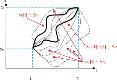
Figure 4: Schematic representation of physical (solid lines) and nonphysical (dashed lines) trajectories in the configuration space $(x,t)$ starting at $(x_{0},t_{0})$ and finishing at $(x\!_{f},t\!_{f})$. In general, Feynman paths $x_{\textit{Fy}}[t]$ do not provide stationary values of the action function, while the quantum (Bohmian) trajectory $x\!_{B}[t]$ provides a stationary value of the quantum action function, $S\!_{B}$ in Eq. (49), and the classical trajectory $x_{cl}[t]$ a stationary value of the classical action function, $S_{cl}$ in Eq. (48).

where $C$ is a normalization constant. It can be demonstrated that the wave function constructed from Eq. (46) with Eq. (47) reproduces the Schrödinger equation om.feynmann1965 . Certainly, Feynamn paths and Bohmian trajectories are completely different. In particular, there is only one Bohmian trajectory $x\!_{B}[t]$ solution of Eq. (39) that goes from point $(x_{0},t_{0})$ to point $(x\!_{f},t\!_{f})$, as seen in Fig. 4, while there are infinite Feynman paths $x_{\textit{Fy}}[t]$ that connect both points. In particular, one of the Feynman paths is certainly the Bohmian trajectory $x\!_{B}[t]$ and another is the classical trajectory $x_{cl}[t]$. In general, $x\!_{B}[t]$ is different from $x_{cl}[t]$. The later is the trajectory that minimizes the classical action function:

$$S(x_{cl}[t];x_{0},t_{0};x_{f},t_{f})=\int_{t_{0}}^{t_{f}}\left[\frac{1}{2m}(\dot{x}[t])^{2}-V(x[t],t)\right]dt$$ (48)

while the former is the trajectory that minimizes the quantum action function:

$$S(x_{B}[t];x_{0},t_{0};x_{f},t_{f})=\!\int_{t_{0}}^{t_{f}}\left[\frac{1}{2m}(\dot{x}[t])^{2}-V(x[t],t)-Q(x[t],t)\right]dt$$ (49)

The derivation of the last expression can be straightforwardly obtained by repeating the steps done from the classical action function to the classical Hamilton–Jacobi equation but using now the quantum Hamilton–Jacobi equation. We conclude that Bohmian trajectories are quite different from Feynman paths. The Bohmian trajectories are part of the basic ontology of the theory, while the Feynman paths are basically a mathematical tool to compute the probabilities.

On the other hand, one could be interested in discussing whether the Feynman approach could be a more useful computational tool than Bohmian mechanics for solving quantum systems. In principle, it seems that Feynman paths would be less practical because we would have to compute an infinite number of trajectories from one particular initial position and then repeat the procedure for all initial positions. On the contrary, in Bohmian mechanics we only need to compute one quantum trajectory for each initial position. See problems 15, 16 and 17.

V.6 Basic postulates for a single-particle

After introducing the reader to the language of trajectories for quantum mechanics (and wave functions for classical mechanics), we can state the basic postulates of the Bohmian theory for a single particle. hey summarize in a few sentences all the discussions held so far. In general, the postulates of any physical theory can be presented in different compatible ways. For example, classical mechanics can be postulated from Newton’s laws or Hamilton’s principle. We follow here the standard presentation of Bohmian mechanics that involves a smaller number of ingredients om.Holand1993 ; om.Valentini2006 ; om.Bohmian1996 ; om.Durrllibre ; om.reviewabc ; om.llibreph .

FIRST POSTULATE: The dynamics of a single particle in a single experiment in a quantum system is defined by a trajectory $x[t]$ that moves continuously under the guidance of a wave function $\psi(x,t)$. The wave function $\psi(x,t)$ is a solution of the Schrödinger equation:

$$i\hbar\frac{\partial\psi(x,t)}{\partial t}=-\frac{\hbar^{2}}{2m}\frac{{\partial}^{2}\psi(x,t)}{\partial x^{2}}+V(x,t)\;\psi(x,t)$$

The trajectory $x[t]$ is obtained by time-integrating the particle velocity $v[t]$ defined as:

$$v(x,t)=\frac{J(x,t)}{|\psi(x,t)|^{2}}$$

where $J(x,t)$ is the (ensemble) current density given by:

$$J(x,t)=i\frac{\hbar}{2m}\left(\psi(x,t)\frac{\partial\psi^{*}(x,t)}{\partial x}-\psi^{*}(x,t)\frac{\partial\psi(x,t)}{\partial x}\right)$$

The initial position $x[t_{0}]$ and velocity $v[t_{0}]$ must be specified to completely determine the trajectory $x[t]$.

SECOND POSTULATE (quantum equilibrium hypothesis): The initial position and velocity of a particular trajectory cannot be known with certainty. When the experiment is repeated many times ( j $=$ 1$,\ldots,$ M), the initial positions $\{x^{j}[t_{0}]\}$ of an ensemble of trajectories $\{x^{j}[t]\}$, associated to the same $\psi(x,t)$, have to satisfy $R^{2}(x,t_{0})=|\psi(x,t_{0})|^{2}$, that is the number of trajectories of the ensemble between $x$ and $x+dx$ at the initial time $t_{0}$ is proportional to $R^{2}(x,t_{0})=|\psi(x,t_{0})|^{2}$. The initial velocity of each trajectory is determined by $v^{j}[t_{0}]=J(x^{j}[t_{0}],t_{0})/|\psi(x^{j}[t_{0}],t_{0})|^{2}$.

The condition on the distribution of the initial position in different experiments can be written mathematically as:

$$R^{2}(x,t_{0})=\lim_{M\rightarrow\infty}\frac{1}{M}\sum_{j=1}^{M}\delta(x-x^{j}[t_{0}])$$ (50)

where $j=1,\ldots,M$ is the index of the different trajectories belonging to different experiments. If the set of $M$ positions of different experiments follows the distribution in Eq. (50) at the initial time $t=0$, it is easy to demonstrate that the distribution of positions satisfies $R(x,t)^{2}=|\psi(x,t)|^{2}$ at any time other time $t$:

$$R^{2}(x,t)=\lim_{M\rightarrow\infty}\frac{1}{M}\sum_{j=1}^{M}\delta(x-x^{j}[t])$$ (51)

provided that the many-particle wave function evolves according to the Schrödinger equation and that the particles move according to the corresponding Bohmian velocity, see problem 7. This property is known as equivariance om.extra9 ; om.llibreph and it is key for the empirical equivalence between Bohmian mechanics and other quantum theories. Eq. (51) says that Born’s law is always satisfied by counting particles om.Holand1993 ; om.Durrllibre ; om.reviewabc ; om.llibreph . Eq. (51) also explains why quantum results are unpredictable at the empirical arena om.randomness .

The second postulate needs some additional remarks. It is argued by some authors that the second postulate, the quantum equilibrium hypothesis, is not a necessary postulate of the Bohmian theory. We will briefly explain the reasons in Sec. VI.5 when dealing with the postulates of a many particle system.

These postulates represent a minimalist explanation of the Bohmian interpretation of quantum mechanics without mentioning either the Hamilton–Jacobi equation, Eq. (39) or the quantum potential, Eq. (40). Certainly, we can formulate Bohmian mechanics without the use of the Hamilton–Jacobi formalism; however, in the authors’ opinion, the quantum Hamilton–Jacobi and the quantum potential allows us to improve our understanding of Bohmian mechanics and provides clear arguments for discussing the similarities and differences between classical and quantum theories. Those who dislike the use of the quantum potential (and the quantum Hamilton–Jacobi equation) argue that it naturally appears in the Schrödinger equation, but it is not present in other wave equations such as Dirac’s one. On the contrary, they state that the concept of Bohmian velocity, as defined in the first postulate, is much more general because it is always present in any wave equation, as far as a local continuity equation for the probability density can be established. This is true. However, in spite of this important limitation, we will show several times in this book that the quantum potential is a quite useful tool.

Finally, let us emphasize that no postulate about measurement is formulated here because, in Bohmian mechanics, no postulate about measurement is needed. For a more detailed explanation, please refer to Refs. om.Holand1993 ; om.Valentini2006 ; om.Bohmian1996 ; om.Durrllibre ; om.reviewabc ; om.llibreph and Sec. VII. In next section, we will explain how these postulates for single-particle systems are generalized to many-particle systems.

VI Bohmian Mechanics for Many-Particle Systems

VI.1 Preliminary discussions: The many body problem

Up to now we have only studied a simple system composed of just one particle. However, a single-particle quantum system is some kind of crude idealization of any macroscopic or microscopic system found in nature, which is usually formed by a very large number of interacting particles. Strictly speaking, a single-particle system cannot be measured (one needs to consider the particles of the measuring apparatus that interact with the single-particle system). In this section we will study nonrelativistic many-particle quantum systems with Bohmian trajectories. First of all, let us clarify the meaning of the term “many-particle” in Bohmian mechanics, as it can easily be misinterpreted. As we have explained in the previous section, we need an infinite ensemble of trajectories, $M\rightarrow\infty$, to describe the statistics of a single-particle quantum system. These different trajectories should not be confused with different physical particles of the system, since they all refer to different realizations (experiments) of the same single-particle quantum system.

Let us consider now a quantum system with $N$ degrees of freedom, that is, an $N$ body quantum system. We will use a particular variable $x_{k}$ for each degree of freedom $k=1,\ldots,N$. The wave function will thus be a function of all $x_{1},\ldots,x_{N}$ variables. Now, a many-particle Bohmian trajectory will involve $N$ interacting physical particles $x_{1}[t],\ldots,x_{N}[t]$. The relevant point that allows us to use the adjective “many-particle” is that the $N$ particles interact between them, that is, the interacting potential depends on all possible particle positions, $V(x_{1},\ldots,x_{N})$, in a non-trivial way. Along this section, in order to simplify our notation, we will use $\vec{x}[t]=(x_{1}[t],\ldots,x_{N}[t])$ or $\vec{x}=(x_{1},\ldots,x_{N})$.

Now, an ensemble of identical experiments will be composed of $M\rightarrow\infty$ Bohmian trajectories $\vec{x}^{j}[t]$, with $j=1,\ldots,M$. The superscript $j$ refers to the statistical index (counting experiments), while the subscript index will refer to each of the $N$ interacting particles present in each experiment, that is, $\vec{x}^{j}[t]=(x^{j}_{1}[t],\ldots,x^{j}_{N}[t])$. In the rest of chapter, we will use $M$ to refer to the number of experiments and $N$ to the number of physical particles of the quantum system in each experiment.

The first step to obtain the many-particle quantum trajectories is solving the following many-particle Schrödinger equation:

$$i\hbar\frac{\partial\psi(\vec{x},t)}{\partial t}=\left(\sum_{k=1}^{N}-\frac{\hbar^{2}}{2m}\frac{\partial^{2}}{\partial x_{k}^{2}}+V(\vec{x},t)\right)\psi(\vec{x},t)$$ (52)

The solution $\psi(\vec{x},t)$ of this equation is the so-called many-particle wave function, that is defined in a $N$-dimensional space (plus time). The problem of $N$ particles in a 1D space is formally equivalent to the one of a single particle in an $N$-dimensional space. Here, we will use the term “many-particle” in a wide sense to include the single-particle $N\geq 2$ dimensional case.

Equation (52) is analitically unsolvable most of the times, and its numerical integration is out of today’s present computer capabilities, even for systems with $N\gtrsim 5$, since we need to compute the wave function $\psi(\vec{x},t)$ in the $N$-dimensional configuration space. Let us roughly estimate the hard disk space that we would require to store $\psi(\vec{x},t)$. Considering, for instance, a system with $N=10$ particles confined in a 1D region of 10 nm, which we discretize with a spatial step of $\Delta x=0.1$ nm, we have a grid of 100 points for each dimension $x_{k}$. Then, the total number of points in the configuration space for the 10 particles is $100^{10}=10^{20}$. Using 4 bytes (32 bits) to store the complex value of the wave function at each grid point, the information contained in a 10-particle wave function would require more than $3\times 10^{8}$ Terabytes (TB) (and more than $3\times 10^{28}$ TB for $20$ particles). This practical limitation is the main reason why our knowledge of many-particle quantum systems is so poor. This difficulty is the so-called many body problem. In 1929, Dirac wrote the following om.dirac1929bis :

The general theory of quantum mechanics is now almost complete. The underlying physical laws necessary for the mathematical theory of a large part of physics and the entire chemistry are thus completely known, and the difficulty is only that the exact application of these laws leads to equations much too complicated to be soluble.

Three decades later, Born rephrased the issue om.born1960bis :

It would indeed be remarkable if Nature fortified herself against further advances in knowledge behind the analytical difficulties of the many body problem.

The adjective “many-particle” can certainly be used with classical mechanics for $N$ particles interacting through $V(\vec{x},t)$. Now, it would be interesting to address the previous problem of storing the state of a 10-particle system but now from the classical mechanics perspective. Solving the problem means finding the many-particle trajectory $\vec{x}^{\rm cl}[t]$. As discussed at the end of subsection 1.2.4, a classical many-particle trajectory can be computed alone, without knowing the rest of the trajectories of the ensemble (with different initial positions). At a computational level, this feature of classical mechanics implies a dramatic simplification. Basically, at each time step of the simulation, if the analytical expression for the potential is known, we just need to save the position and velocity of each particle. This means 20 real values for the 10-particle systems mentioned above. The classical trajectory of each particle, $x^{\rm cl}_{k}[t]$, can be obtained by solving a coupled system of Newton’s second laws:

$$m_{k}\frac{d^{2}x^{\rm cl}_{k}[t]}{dt^{2}}=\left[-\frac{\partial V(\vec{x},t)}{\partial x_{k}}\right]_{\vec{x}=\vec{x}^{\rm cl}[t]}$$ (53)

Fortunately, to compute a single classical trajectory $\vec{x}^{\rm cl}[t]$, we only need to evaluate the derivative of the many-particle potential $V(\vec{x},t)$ along the trajectory. In the quantum case, even finding a single trajectory means solving for the entire wave function $\psi(\vec{x},t)$ that encapsulates the information of the entire ensemble of trajectories of all other experiments (the quantum wholeness).

In the scientific literature, there are many attempts to provide reasonable approximations to the many-body quantum problem. Density functional theory om.kohn1964 ; om.kohn1965 and the Hartree–Fock approximation om.Hartree ; om.Hartree2 ; om.Fock are some of the most popular techniques among the scientific community for dealing with the many body problem. In Sec. VI.1 we will discuss whether Bohmian trajectories can help in solving the many body problem. In what follows, we present the basic theory of the many-particle Bohmian trajectories.

VI.2 Many-particle quantum trajectories

The efforts done in the single-particle section to compare classical and quantum mechanics are valid here. In particular, we could write a classical (many-particle) wave equation or develop (many-particle) trajectories for quantum systems. In this section, we will only explicitly develop the latter. We start by considering (nonrelativistic) spinless particles. In Sec. VI.4 we will introduce spin.

VI.2.1 Many-particle continuity equation

Following a similar development as we did for the single-particle case, see Sec. V.3, we can derive the following local continuity equation associated to the many-particle Schrödinger equation, Eq. (52):

$$\frac{\partial|\psi(\vec{x},t)|^{2}}{\partial t}+\sum_{k=1}^{N}\frac{\partial}{\partial x_{k}}J_{k}(\vec{x},t)=0$$ (54)

where we have defined

$$J_{k}(\vec{x},t)=i\frac{\hbar}{2m}\left(\psi(\vec{x},t)\frac{\partial\psi^{*}(\vec{x},t)}{\partial x_{k}}-\psi^{*}(\vec{x},t)\frac{\partial\psi(\vec{x},t)}{\partial x_{k}}\right)$$ (55)

as the $k$-th component of the current density, see problem 7.

Since the many-particle Schrödinger equation is also compatible with a local conservation of particles, we can interpret $|\psi(\vec{x},t)|^{2}$ as the spatial distribution of an ensemble of many-particle trajectories assigned to an ensemble of different experiments. The Bohmian velocity of the $k$-th trajectory is:

$$v_{k}(\vec{x},t)=\frac{J_{k}(\vec{x},t)}{|\psi(\vec{x},t)|^{2}}$$ (56)

In fact, the strategy followed here to develop Bohmian mechanics can be extended to any quantum equation of motion where a continuity equations holds: first, look for a continuity equation for the probability density and, then, define a velocity for the Bohmian trajectories as the current density divided by the probability density. A particular example will be developed for particles with spin in Sec. VI.4 and chapter 8.

VI.2.2 Many-particle quantum Hamilton–Jacobi equation

Alternatively, we can obtain Bohmian mechanics from a quantum Hamilton–Jacobi equation. We start by introducing the polar form of the many-particle wave function $\psi(\vec{x},t)=R(\vec{x},t)e^{iS(\vec{x},t)/\hbar}$ into the many-particle Schrödinger equation, Eq. (52). Then, after a quite simple manipulation, one obtains from the imaginary part:

$$\frac{\partial R^{2}(\vec{x},t)}{\partial t}+\sum_{k=1}^{N}\frac{\partial}{\partial x_{k}}\left(\frac{1}{m}\frac{\partial S(\vec{x},t)}{\partial x_{k}}R^{2}(\vec{x},t)\right)=0$$ (57)

where we recognize the velocity of the $k$-th particle as:

$$v_{k}(\vec{x},t)=\frac{1}{m}\frac{\partial S(\vec{x},t)}{\partial x_{k}}$$ (58)

Equations (56) and (58) are identical. This is shown in problem 6 for a 1D system, but it can straightforwardly be generalized to $N$ dimensions. The real part of the Schrödinger equation leads to a many-particle version of the quantum Hamilton–Jacobi equation:

$$\frac{\partial S(\vec{x},t)}{\partial t}+\sum_{k=1}^{N}\frac{1}{2m}\left(\frac{{\partial}S(\vec{x},t)}{\partial x_{k}}\right)^{2}+V(\vec{x},t)+Q(\vec{x},t)=0$$ (59)

where we have defined the quantum potential as:

$$Q(\vec{x},t)=\sum_{k=1}^{N}Q_{k}(\vec{x},t)$$ (60)

with:

$$Q_{k}(\vec{x},t)=-\frac{\hbar^{2}}{2m}\frac{{\partial}^{2}R(\vec{x},t)/\partial x^{2}_{k}}{R(\vec{x},t)}$$ (61)

Again, we can obtain a system of coupled Newton-like equations (one for each component of $\vec{x}$) for the many-particle Bohmian trajectories by computing the time-derivative of the Bohmian velocity of Eq. (56):

$$m\frac{d^{2}x_{k}[t]}{dt^{2}}=\left[-\frac{\partial}{\partial x_{k}}\left(V(\vec{x},t)+Q(\vec{x},t)\right)\right]_{\vec{x}=\vec{x}[t]}$$ (62)

Both the potential $V(\vec{x},t)$ and the quantum potential $Q(\vec{x},t)$ introduce correlations between particles. All physical interactions are essentially expressed as correlations (relations) between the degrees of freedom. In the following, we will discuss some important differences between classical and quantum correlations.

VI.3 Factorizability, entanglement, and correlations

There are important differences between the correlations introduced by the classical potential $V(\vec{x},t)$ and the quantum potential $Q(\vec{x},t)$:

1. In general, the term $V(\vec{x},t)$ decreases with the distance between particles. A simple example is the Coulomb interaction. However, $Q(\vec{x},t)$ depends only on the shape of the wave function, not on its value (see Eq. (61)). Thus, the quantum potential that we would obtain from Eq. (61) using either $R(\vec{x},t)$ or $aR(\vec{x},t)$ would be exactly the same, even when $a\rightarrow 0$. Thus, the quantum potential can produce a significative interaction between two particles, even if they are very far apart.

2. In general, the term $V(\vec{x},t)$ produces classical correlations between different particles. The particular dependence of $V(\vec{x},t)$ in all variables $x_{1},\ldots,x_{N}$ imposes a restriction on the speed of the interaction. The variations of $x_{i}$ can only affect $x_{j}$ after a time larger than $|x_{i}-x_{j}|/c$, $c$ being the speed of light. For example, the relation between the particles positions in the electromagnetic interactions ensures that there is no superluminal influence between particles. However, such a restriction is not present in the quantum potential. Thus, very far particles have an instantaneous (nonlocal) interaction between them.

The quantum potential is at the origin of all quantum correlations, that is, entanglement, that can imply (nonlocal) faster-than-light interactions when two distant particles are involved. As mentioned in Sec. IV.5, this “spooky action at a distance” is what bothered Einstein about Bohmian mechanics (and quantum mechanics, in general). In 1964, Bell elaborated his famous theorem that established clear experimentally testable mathematical inequalities that would be fulfilled by local theories but would be violated by nonlocal ones om.Bell1964 . All experimental results obtained so far confirm that Bell’s inequalities are violated. Therefore, contrarily to Einstein’s belief, we have to accept the real existence, in nature, of faster-than-light causation. Entanglement is an intrinsic correlation in quantum mechanics (whose complexity and potentialities eventually come from the fact that a $N$-particle wave function lives in a $N$-dimensional configuration space) and is at the core of quantum information science, which makes teleportation, quantum communication, quantum cryptography, and quantum computing possible.

To improve our understanding of correlations, let us discuss under which conditions we cannot expect correlations between $N$ particles. Let us focus our attention on a wave function $\psi(\vec{x},t)$ that can be written as a product of single-particle wave functions associated with each of the particles:

$$\psi(\vec{x},t)=\prod_{k=1}^{N}\psi_{k}(x_{k},t)$$ (63)

We call such a wave function “factorizable” or “separable”. Equation (63) expresses the physical independence of the $N$ particles (even though the wave functions $\psi_{k}(x_{k},t)$ may overlap). According to Born’s statistical interpretation of wave functions, the squared modulus of a wave function is the probability density of the quantum particle; thus the quantum wave function, Eq. (63), corresponds to a system without (classical or quantum) correlations between particles. It is well known that such a solution occurs when the potential in Eq. (52) can be written as $V(\vec{x})=\sum_{k}V_{k}(x_{k})$. Next, let us reformulate this result with Bohmian trajectories.

We realize that the phase and modulus of Eq. (63) are given by:

$$S(\vec{x},t)=\sum_{k=1}^{N}S_{k}(x_{k},t)$$ (64)

and

$$R(\vec{x},t)=\prod_{k=1}^{N}R_{k}(x_{k},t)$$ (65)

by defining

$$\psi_{k}(x_{k},t)=R_{k}(x_{k},t)e^{iS_{k}(x_{k},t)/\hbar}$$ (66)

In this case, the many-particle quantum potential can be written as:

$$Q_{k}(\vec{x},t)=-\frac{\hbar^{2}}{2m}\frac{{\partial}^{2}R_{k}(x_{k},t)/\partial x^{2}_{k}}{R_{k}(x_{k},t)}$$ (67)

Then, we can easily deduce from Eq. (59) that each $\psi_{k}(x_{k},t)$ is a solution of the following single-particle quantum Hamilton–Jacobi equation:

$$\frac{\partial S_{k}(x_{k},t)}{\partial t}+\frac{1}{2m}\left(\frac{{\partial}S_{k}(x_{k},t)}{\partial x_{k}}\right)^{2}+V(x_{k},t)+Q_{k}(x_{k},t)=0$$ (68)

In addition, each $\psi_{k}(x_{k},t)$ satisfies a conservation law:

$$\frac{\partial R_{k}^{2}(x_{k},t)}{\partial t}+\frac{\partial}{\partial x_{k}}\left(\frac{1}{m}\frac{\partial S_{k}(x_{k},t)}{\partial x_{k}}R_{k}^{2}(x_{k},t)\right)=0$$ (69)

From these equations we can easily deduce an independent guiding equation for each $k$-particle:

$$m\frac{dx_{k}[t]}{dt}=\left(\frac{\partial S_{k}(x_{k},t)}{\partial x_{k}}\right)_{x_{k}=x_{k}[t]}$$ (70)

showing the absence of correlations between (the different components of the many-particle) Bohmian trajectory.

VI.4 Spin and identical particles

Elementary particles, such as electrons or quarks, have spin, an internal (discrete) degree of freedom that can influence their quantum dynamics in a nontrivial manner. In this section we will briefly explain how to extend (nonrelativistic) Bohmian mechanics to include spin.

VI.4.1 Single-particle with s $=$ 1/2

In the orthodox formulation of quantum mechanics, the state of a single particle with spin $s$ is described by a $2s+1$ component vector of wave functions with:

$$\vec{\Psi}(\vec{r},t)=\left(\begin{array}[]{c}\Psi_{1}(\vec{r},t)\\ \vdots\\ \Psi_{2s+1}(\vec{r},t)\end{array}\right)$$ (71)

where $\vec{r}=(x_{1},x_{2},x_{3})$ represents the 3D position of the particle. The time evolution of this state is no longer governed by the Schrödinger equation but by more involved wave equations such as the Pauli equation for $s={1}/{2}$ om.landaulif ; om.ward ; om.colijn2002 .

The strategy to find Bohmian trajectories for spin particles will be the following: we will look for a continuity equation of the probability density and define the Bohmian velocity as the current density divided by the probability density. The idea is quite simple, but the mathematical development can be much more complicated. Therefore, we will focus on a particular example for a spin $s=1/2$ charged particle, whose vectorial wave function,

$$\vec{\Psi}(\vec{r},t)=\left(\begin{array}[]{c}\Psi_{\uparrow}(\vec{r},t)\\ \Psi_{\downarrow}(\vec{r},t)\end{array}\right)$$ (72)

has two components and it is called a spinor. In this particular case, the spin along a particular direction takes only two possible values, referred to as spin-up ($\uparrow$) and spin-down ($\downarrow$) states. The time evolution is given by the Pauli equation om.ward :

$$i\hbar\frac{\partial}{\partial t}\vec{\Psi}(\vec{r},t)=\left[\frac{1}{2m}\vec{\sigma}\cdot\left(-i\hbar\vec{\nabla}-q\vec{A}(\vec{r},t)\right)^{2}+V(\vec{r},t)\right]\vec{\Psi}(\vec{r},t)$$ (73)

where $\vec{\sigma}=(\sigma_{1},\sigma_{2},\sigma_{3})$ is a vector containing the Pauli matrices om.landaulif :

$$\sigma_{1} = \begin{pmatrix}0&1\\ 1&0\end{pmatrix}$$ (74)

$$\sigma_{2} = \begin{pmatrix}0&-i\\ i&0\end{pmatrix}$$ (75)

$$\sigma_{3} = \begin{pmatrix}1&0\\ 0&-1\end{pmatrix}$$ (76)

and $V(\vec{r},t)/q$ and $\vec{A}(\vec{r},t)=(A_{1}(\vec{r},t),A_{2}(\vec{r},t),A_{3}(\vec{r},t))$ are, respectively, the electromagnetic scalar and vector potential.

From the Pauli equation we obtain a continuity equation:

$$\frac{\partial\rho(\vec{r},t)}{\partial t}+\vec{\nabla}\vec{J}(\vec{r},t)=0$$ (77)

with the probability and current densities defined as:

$$\rho(\vec{r},t) = \vec{\Psi}^{\dagger}(\vec{r},t)\cdot\vec{\Psi}(\vec{r},t)$$ (78)

$$\vec{J}(\vec{r},t) = i\frac{\hbar}{2m}\left(\vec{\Psi}(\vec{r},t)\cdot{\vec{\nabla}\vec{\Psi}^{\dagger}(\vec{r},t)}-\vec{\Psi}^{\dagger}(\vec{r},t)\cdot{\vec{\nabla}\vec{\Psi}(\vec{x},t)}\right)-\frac{\vec{A}(\vec{r},t)}{mc}\rho(\vec{r},t),$$ (79)

where $\vec{\Psi}^{\dagger}$ denotes the conjugate transpose of $\vec{\Psi}$.

Defining the Bohmian velocity as:

$$\vec{v}(\vec{r},t)=\frac{\vec{J}(\vec{r},t)}{\rho(\vec{r},t)}$$ (80)

one can develop Bohmian trajectories for spin particles. Notice that the spin is basically a property defined through the wave function of the particle, not through its position. In any case, since the Bohmian velocity of the particle is affected by the wave function, the spin can have a direct effect on the trajectory. It is out of the scope of this book to further develop Bohmian mechanics for the Pauli equation. In any case, practical examples of the particle trajectories for spin-1/2 particles can be found in Refs. om.Holland2003 ; om.colijn2002 .

The Pauli equation can be rewritten as:

$$i\hbar\frac{\partial}{\partial t}\vec{\Psi}(\vec{r},t) = \left[\frac{1}{2m}\left(-i\hbar\vec{\nabla}-q\vec{A}(\vec{r},t)\right)^{2}-\frac{\hbar q}{2m}\vec{\sigma}\cdot\vec{B}(\vec{r},t)\right.+V(\vec{r},t)\bigg{]}\vec{\Psi}(\vec{r},t)$$ (81)

$\vec{B}(\vec{r},t)=\vec{\nabla}\times\vec{A}(\vec{r},t)$ being the magnetic field. Note that the only term that can transfer population between spin states is the one with $\vec{B}$ (the so-called Stern–Gerlach term). If this term can be neglected then each spin component of Eq. (81) reduces to the familiar Schrödinger equation.

On the other hand we can also consider the case where the Hamiltonian is separable into a part depending only on the particle position and a part depending only on the spin. Then if the initial state is:

$$\vec{\Psi}(\vec{r},0)=\psi(\vec{r},0)\left(\begin{array}[]{c}\alpha_{\uparrow}(0)\\ \alpha_{\downarrow}(0)\end{array}\right)$$ (82)

at later times one can write the spinor evolution in a simpler form as:

$$\vec{\Psi}(\vec{r},t)=\psi(\vec{r},t)\left(\begin{array}[]{c}\alpha_{\uparrow}(t)\\ \alpha_{\downarrow}(t)\end{array}\right)\equiv\psi(\vec{r},t)\vec{\chi}(t)$$ (83)

where $\psi(\vec{r},t)$ depends only on the coordinate of the particles and the function $\vec{\chi}(t)$ depends only on its spin. We call the former the coordinate or orbital wave function and the latter the spin wave function. In this case, the evolution of $\vec{\chi}(t)$ and $\psi(\vec{r},t)$ is independent. If we are not interested in the actual spin of the particles, we can just consider the dynamics of the coordinate function $\psi(\vec{r},t)$, which will be determined by the Schrödinger equation.

VI.4.2 Many-particle system with s $=$ 1/2 particles

For a nonrelativistic system of many particles, where the orbital and spin contributions of the Hamiltonian are initially separable, the many-particle wave function will be also separable at all times, that is:

$$\Psi(\vec{r}_{1},\ldots\vec{r}_{N},t)=\psi(\vec{r}_{1},\ldots\vec{r}_{N},t)\vec{\chi}(t)$$ (84)

where $\psi(\vec{r}_{1},\ldots\vec{r}_{N},t)$ is the time evolution of the orbital state, the solution of the many-particle Schrödinger equation, and $\vec{\chi}(t)$ is the time evolution of the spin part of the system state:

$$\vec{\chi}(t)=\left(\begin{array}[]{c}\alpha_{\uparrow_{1}\uparrow_{2}\ldots\uparrow_{N}}(t)\\ \alpha_{\uparrow_{1}\uparrow_{2}\ldots\downarrow_{N}}(t)\\ \vdots\\ \alpha_{\downarrow_{1}\downarrow_{2}\ldots\downarrow_{N}}(t)\end{array}\right)=\left(\begin{array}[]{c}\alpha_{1}(t)\\ \alpha_{2}(t)\\ \vdots\\ \alpha_{W}(t)\end{array}\right)$$ (85)

$W\equiv(2s+1)^{N}$ is the number of possible combinations of spin projections in one direction for all the particles in the system.

In many practical situations, we are only interested in the evolution of the orbital wave function through the many-particle Schrödinger equation. However, even in this case, there is a peculiar dependence of the dynamics of the particles on the total spin. As explained in many textbooks, there is a pure quantum interaction between identical particles, named “exchange interaction” om.sakurai94 ; om.landaulif . This interaction is not classical, and we cannot find a term in the potential energies of the many-particle Hamiltonian of the Schrödinger equation that accounts for it. Alternatively, this new interaction is introduced in the “shape” of the global wave function, through the requirement of a particular symmetry. We say that a many-particle wave function is anti-symmetric when the interchange of the position and spin degrees of freedom associated to two identical fermions (e.g., electrons) results only in a change of the sign of the global wave function, $\vec{\Psi}(\vec{r}_{1},\vec{r}_{2},\ldots,\vec{r}_{N},t)$. Analogously, we say that the many-particle wave function is symmetric when it remains unchanged after the interchange of the degrees of freedom of two identical bosons.

The crucial point why we cannot forget about spin when dealing with many-particle Hamiltonians is that for separable wave functions, for example, Eq. (84), the symmetry of the orbital part depends on the symmetry of the spin part. For example, since the total wave function must be antisymmetric, two electrons can have a symmetric orbital part if the spin part is antisymmetric, and vice versa. In general, note that the wave function is not separable, and it makes no sense to talk about the symmetry of the orbital and spin parts alone but only of the symmetry of the total wave function. We see that the exchange interaction induces correlations between particles by imposing symmetries (or shapes) to their many-particle wave function.

A standard claim in many quantum mechanics textbooks is that identical particles, for example, two electrons with an antisymmetric wave function, are indistinguishable. It is affirmed that if the particles would have trajectories, they would automatically be distinguishable. In Bohmian mechanics, even with the symmetrization postulate, the adjective “indistinguishable” is inappropriate because one can label one particle’s trajectory $\vec{r}_{1}[t]$ and the other $\vec{r}_{2}[t]$ and thus distinguish them perfectly at the ontological staff.

Bohmian trajectories can actually help us improve our understanding of the symmetrization postulate. Let us assume a two-electron system with an antisymmetric orbital wave function $\psi(\vec{r}_{1},\vec{r}_{2},t)$. We assume that an electron labeled $1$ with the initial position $\vec{r_{1}}[0]$ evolves into $\vec{r_{1}}[t]$ and an another electron labeled $2$ evolves from $\vec{r_{2}}[0]$ to $\vec{r_{2}}[t]$. Then, it can be easily understood that $\vec{r_{1}}^{\prime}[0]=\vec{r_{2}}[0]$ evolves into $\vec{r_{1}}^{\prime}[t]=\vec{r_{2}}[t]$ and $\vec{r_{2}}^{\prime}[0]=\vec{r_{1}}[0]$ evolves into $\vec{r_{2}}^{\prime}[t]=\vec{r_{1}}[t]$. We use primes to notice that $\vec{r_{1}}[t]$ and $\vec{r_{1}}^{\prime}[t]$ correspond to trajectories of the same particle with different initial positions ($\vec{r_{1}}[0]$ or $\vec{r_{2}}[0]$). This result follows from the symmetry of the velocity, that is, the symmetry of the current density and modulus, when positions of the two electrons are interchanged. In summary, Bohmian trajectories of identical particles are clearly distinguishable in our computation, but the observable (ensemble) results obtained from them are indistinguishable when we interchange their initial positions. Hence in Bohmian mechanics a set of particles with exchange symmetry are perfectly distinguishable at the ontological plane, while they become indistinguishable at the empirical plane.

VI.5 Basic postulates for many-particle systems

The basic postulates of Bohmian mechanics for many-particle systems are exactly the same as those we have developed for a single particle but adding the symmetrization postulate. As done in Sec. V.6, we also present a minimalist formulation of the postulates.

In order to simplify our description, we assume the simpler many-particle wave function written as:

$$\vec{\Psi}(\vec{r}_{1},\ldots,\vec{r}_{N},t)=\psi(\vec{r}_{1},\ldots,\vec{r}_{N},t)\left(\begin{array}[]{c}\uparrow_{1}\uparrow_{2}\ldots\uparrow_{N}(t)\\ 0\\ \vdots\\ 0\end{array}\right)$$ (86)

The generalization of the present postulates to include the more general wave functions of Eq. (84) follows straightforwardly.

FIRST POSTULATE: The dynamics of a many-particle quantum system comprises a wave function, Eq. (86), whose orbital part $\psi(\vec{r}_{1},\vec{r}_{2},\ldots,\vec{r}_{N},t)$ is defined in the configuration space $\{\vec{r}_{1},\vec{r}_{2},\ldots,\vec{r}_{N}\}$ plus time, and a many-particle trajectory $\{\vec{r}_{1}[t]$, $\vec{r}_{2}[t],\ldots,\vec{r}_{N}[t]\}$ that moves continuously under the guidance of the wave function.

The orbital part of the wave function $\psi(\vec{r}_{1},\vec{r}_{2},\ldots,\vec{r}_{N},t)$ is a solution of the many-particle Schrödinger equation:

$$i\hbar\frac{\partial\psi(\vec{r}_{1},\ldots,\vec{r}_{N},t)}{\partial t} = \left(\sum_{k=1}^{N}-\frac{\hbar^{2}}{2m}\nabla^{2}_{\vec{r}_{k}}\right.+\ \ V(\vec{r}_{1},\ldots,\vec{r}_{N},t)\Bigg{)}\psi(\vec{r}_{1},\ldots,\vec{r}_{N},t)$$

Each component $\vec{r}_{k}[t]$ of the many-particle trajectory $\{\vec{r}_{1}[t],\ldots,\vec{r}_{N}[t]\}$ is obtained by time-integrating the particle velocity $\vec{v}_{k}[t]=\vec{v}_{k}(\vec{r}_{1},\ldots,\vec{r}_{N},t)$ defined from:

$$\vec{v}_{k}(\vec{r}_{1},\ldots,\vec{r}_{N},t)=\frac{\vec{J}_{k}(\vec{r}_{1},\ldots,\vec{r}_{N},t)}{|\psi(\vec{r}_{1},\ldots,\vec{r}_{N},t)|^{2}}$$

where $|\psi(\vec{r}_{1},\ldots,\vec{r}_{N},t)|^{2}=\psi(\vec{r}_{1},\ldots,\vec{r}_{N},t)\psi^{*}(\vec{r}_{1},\ldots,\vec{r}_{N},t)$ is the square modulus of the wave function and $\vec{J}_{k}=\vec{J}_{k}(\vec{r}_{1},\ldots,\vec{r}_{N},t)$ is the k-particle current density:

$$\vec{J}_{k} = i\frac{\hbar}{2m}\Big{(}\psi(\vec{r}_{1},..,\vec{r}_{N},t)\vec{\nabla}_{\vec{r}_{k}}{\psi^{*}(\vec{r}_{1},..,\vec{r}_{N},t)}-\psi^{*}(\vec{r}_{1},..,\vec{r}_{N},t)\vec{\nabla}_{\vec{r}_{k}}\psi(\vec{r}_{1},..,\vec{r}_{N},t)\Big{)}$$

The initial positions $\{\vec{r}_{10},\vec{r}_{20},\ldots,\vec{r}_{N0}\}$ and velocities $\{\vec{v}_{10}$, $\vec{v}_{20},\ldots$, $\vec{v}_{N0}\}$ have to be specified in order to completely determine the many-particle trajectory.

SECOND POSTULATE (quantum equilibrium hypothesis): The initial positions $\{\vec{r}^{j}_{1}[t_{0}],\vec{r}^{j}_{2}[t_{0}],\ldots,\vec{r}^{j}_{N}[t_{0}]\}$ and velocities $\{\vec{v}^{j}_{1}[t_{0}],\vec{v}^{j}_{2}[t_{0}],\ldots$, $\vec{r}^{j}_{N}[t_{0}]\}$ of a particular many-particle $j$ trajectory cannot be known with certainty. When the experiment is repeated many times, these initial positions of an ensemble of trajectories associated with the same $\psi(\vec{r}_{1},\ldots,\vec{r}_{N},t)$ satisfy that the number of trajectories of the ensemble between $(\vec{r}_{1},\ldots,\vec{r}_{N})$ and $(\vec{r}_{1}+d\vec{r}_{1},\ldots,\vec{r}_{N}+d\vec{r}_{N})$ at the initial time $t_{0}$ is proportional to $R^{2}(\vec{r}^{j}_{1}[t_{0}],\ldots,\vec{r}^{j}_{N}[t_{0}])=|\psi(\vec{r}^{j}_{1}[t_{0}],\ldots,\vec{r}^{j}_{N}[t_{0}],t_{0})|^{2}$. The initial velocity is determined by $\vec{v}_{k}^{j}[t_{0}]=\vec{J}_{k}(\vec{r}^{j}_{1}[t_{0}],\ldots,\vec{r}^{j}_{N}[t_{0}],t_{0})/|\psi(\vec{r}^{j}_{1}[t_{0}],\ldots,\vec{r}^{j}_{N}[t_{0}],t_{0})|^{2}$ .

The condition on the initial position can be written mathematically as:

$$R^{2}(\vec{r}_{1},\ldots,\vec{r}_{N},t_{0})=\lim_{M\rightarrow\infty}\frac{1}{M}\sum_{j=1}^{M}\prod_{k=1}^{N}\delta(\vec{r}-\vec{r}_{k}^{j}[t_{0}])\;\;{\rm for}\;t=t_{0}$$ (87)

Notice the presence of two indices, the $j=1,\ldots,M$ for the infinite ensemble of identical experiments and the $k=1,\ldots,N$ for the $N$ degrees of freedom.

THIRD POSTULATE (symmetrization postulate of quantum mechanics): If the variables $\vec{r}_{i},\uparrow_{i}$ and $\vec{r}_{j},\uparrow_{j}$ refer to two identical particles of the ensemble, then the wave function, Eq. (86), is either symmetric:

$$\psi(.,\vec{r}_{i},.,\vec{r}_{j},.,t)\!\!\left(\begin{array}[]{c}\uparrow_{i}\ldots\uparrow_{j}\ldots\\ 0\\ \vdots\\ 0\end{array}\right)=\psi(.,\vec{r}_{j},.,\vec{r}_{i},.,t)\left(\begin{array}[]{c}\uparrow_{j}\ldots\uparrow_{i}\ldots\\ 0\\ \vdots\\ 0\end{array}\right)$$ (88)

if the particles are bosons (every particle with an integer spin 0, 1, 2, …is a boson), or antisymmetric:

$$\psi(.,\vec{r}_{i},.,\vec{r}_{j},.,t)\!\!\left(\begin{array}[]{c}\uparrow_{i}\ldots\uparrow_{j}\ldots\\ 0\\ \vdots\\ 0\end{array}\right)\!\!=-\psi(.,\vec{r}_{j},.,\vec{r}_{i},.,t)\!\!\left(\begin{array}[]{c}\uparrow_{j}\ldots\uparrow_{i}\ldots\\ 0\\ \vdots\\ 0\end{array}\right)$$ (89)

if the particles are fermions (every particle with a half-odd spin 1/2, 3/2, …is a fermion). In Eq. (88) and Eq. (89) it is understood that all other degrees of freedom of the other particles remain unchanged.

As we already did in the development of the postulates for a single-particle system, we remind that the second postulate needs some additional remarks since it has been argued by some authors that this postulate, the quantum equilibrium hypothesis, is not a necessary postulate of the Bohmian theory.

First, it has been demonstrated that if one assumes that the many-particle wave function of the whole Universe, the so-called Universal wave function that includes all degrees of freedom of the Universe, satisfies some (typical) conditions then, it follows that each (conditional) wave function of each quantum (sub) system will satisfy its own Eq. (87). Thus, the justification about the quantum equilibrium postulate has to be done only for the Universal wave function, not for each individual (sub)system.

Probably, the most accepted view against taking the quantum equilibrium as a postulate comes from the seminal work by Dürr, Goldstein, and Zanghì om.extra9 ; om.llibreph , where the equivariance in any system is discussed from the initial configurations of (Bohmian) particles in the Universe. Using Bohmian mechanics to describe the wave function of the whole Universe, then the wave function associated to any (sub)system is an effective (conditional) wave function of the universal one. Using typicality arguments, they showed that the overwhelming majority of possible selections of initial positions of particles in the Universe will satisfy Eq. (87) in a subsystem (or Eq. (51) for a subsystem with one degree of freedom) om.extra9 ; om.llibreph . Other authors om.towler2011 have attempted to dismiss Eq. (87) as a postulate by showing that any initial configuration of Bohmian particles will relax, after some time, to a distribution very close to Eq. (51) for a subsystem. Such discussions about quantum equilibrium are far from the scope of this book. Therefore, from a practical point of view, one can postulate Eq. (87) (at some initial time) in the Bohmian theory in the same way that Born’s law is a postulate in the orthodox theory.

Again, no postulate about measurement is needed, since in Bohmian mechanics measurement is treated as a particular case of interaction between particles (see Sec. VII).

VI.6 The conditional wave function: many-particle Bohmian trajectories without the many-particle wave function

In section 1.2.4, when discussing the similarities and differences between classical and quantum mechanics, we mentioned quantum wholeness (the dependence of each individual Bohmian trajectory on the rest of trajectories through the wave function) as a fundamental difference. This concept acquires an even more dramatic meaning when dealing with many-body systems. A particular Bohmian trajectory of the $k$-particle $\vec{r}_{k}^{j}[t]$ depends on the rest of infinite $j=1,\ldots,M$ possible trajectories (with different initial position associated to different experiments) of all $k=1,\ldots,N$ particles (corresponding to the $N$ degrees of freedom of the quantum system). This property is mathematically manifested by the fact that the many-particle wave function is defined in an $N$-dimensional configuration space rather than in the usual real 3D real space. In a 3D real space one can easily define whether or not two particles are far away. In general, the potential profile that determines the interaction between these two particles decreases with the distance. However, two distant particles that share a common region of the $N$-dimensional configuration space where the wave function is different from zero have an interaction (entanglement) independently of their distance.

As discussed in section Sec. VI.1, the need of computing the many-particle wave function in the $N$-dimensional configuration space is the origin of the quantum many-body problem. Among the large list of approximations present in the literature to tackle this problem, Bohmian mechanics provides a natural, original and mainly unexplored solution through the use of the conditional wave function om.norsen . Due to the Bohmian dual description of a quantum system as particles and waves, one can reduce the complexity of a many-particle wave function through the substitution of some of the $N$ degrees of freedom by its corresponding Bohmian trajectories. The new wave function with a reduced number of degrees of freedom is named conditional wave function. For a discussion about the fundamental implications of working with conditional wave functions instead of full many-body wave functions, see Refs om.norsen ; om.norsen2 . We will present now some work on the computational abilities of such conditional wave functions.

Hereafter, for simplicity, we return to a definition of the degrees of freedom of the many-particle quantum system in terms of $\{x_{1},x_{2},\ldots,x_{N}\}$ instead of $\{\vec{r}_{1},\vec{r}_{2},\ldots,\vec{r}_{N}\}$. The direct solution of the many-particle Schrödinger equation, Eq. (52), is intractable numerically. On the contrary, differential classical equations of motion deal with solutions in a much smaller configuration space, $\{x_{1}[t],\ldots,x_{i-1}[t],x_{a},x_{i1}[t],\ldots,x_{N}[t]\}$, where all other trajectories are known parameters, except $x_{a}$. In other words, the Newton solution of $x_{a}[t]$ just needs the spatial dependence of $V(x_{1}[t],\ldots,x_{a},\ldots,x_{N}[t])$ on the variable $x_{a}$. In this section, we summarize the formalism developed by Oriols om.oriolsprl to compute many-particle Bohmian trajectories without knowing the many-particle wave function. It is a clear example of how Bohmian mechanics can be a powerful computational tool.

The main idea behind the work developed in om.oriolsprl is that any Bohmian trajectory $x_{a}[t]$ that is computed from the many-particle wave function $\Psi(\vec{x},t)$ solution of Eq. (52) can be alternatively computed from a much simpler single-particle conditional wave function $\phi_{a}(x_{a},t)=\Psi(x_{a},\vec{x}_{b}[t],t)$. Here, we use the notation $\vec{x}=\{x_{a},\vec{x}_{b}\}$ with $\vec{x}_{b}=\{x_{1},\ldots,x_{a-1},x_{a+1},\ldots,x_{N}\}$ for particle positions and $\vec{x}_{b}[t]=\{x_{1}[t],\ldots,x_{a-1}[t],x_{a+1}[t],\ldots,x_{N}[t]\}$ for Bohmian trajectories.

It is quite trivial to demonstrate the ability of $\phi_{a}(x_{a},t)$ in reproducing $x_{a}[t]$. By construction, when we use a polar form $\phi_{a}(x_{a},t)=r_{a}(x_{a},t)\;e^{i\;s_{a}(x_{a},t)/\hbar}$, the angle $s_{a}(x_{a},t)$ is identical to the angle $S(x_{a},\vec{x}_{b},t)$ of $\Psi(x_{a},\vec{x}_{b},t)$ evaluated at $\{x_{a},\vec{x}_{b}[t]\}$. Therefore, since the velocity of the trajectory $x_{a}[t]$ is computed from the spatial dependence of $S(x_{a},\vec{x}_{b},t)$ on $x_{a}$ when all other positions are fixed at $\vec{x}_{b}=\vec{x}_{b}[t]$, the same velocity will be obtained from the spatial dependence of $s_{a}(x_{a},t)$. Interestingly, $\phi_{a}(x_{a},t)$ is solution of a single-particle (pseudo) Schrödinger equation because it depends only on time $t$ and position $x_{a}$. Next, our effort will be focused on determining such single-particle equations.

VI.6.1 Single-particle pseudo-Schrödinger equation for many-particle systems

First of all, we show that any (totally arbitrary) single-valued complex function $\phi_{a}(x_{a},t)$, which has a well-defined second-order spatial derivative and first-order temporal derivative, can be obtained from a Schrödinger-like equation when the following potential $W(x_{a},t)$ is used:

$$W(x_{a},t)=\frac{i\hbar\frac{\partial\phi_{a}(x_{a},t)}{\partial t}+\frac{\hbar^{2}}{2m}\frac{\partial^{2}\phi_{a}(x_{a},t)}{\partial_{x_{a}}^{2}}}{\phi_{a}(x_{a},t)}$$ (90)

For an arbitrary (complex) function, the potential energy $W(x_{a},t)$ can be complex, too. In fact, we are interested in rewriting $W(x_{a},t)$ in terms of the polar form of the wave function $\phi_{a}(x_{a},t)=r_{a}(x_{a},t)\;e^{i\;s_{a}(x_{a},t)/\hbar}$. We obtain for the real part:

$${Real}[W(x_{a},t)] = -\Bigg{(}\frac{1}{2\;m}\left(\frac{\partial s_{a}(x_{a},t)}{\partial x_{a}}\right)^{2}-\frac{\hbar^{2}}{2\;m\;r_{a}(x_{a},t)}\frac{\partial^{2}r_{a}(x_{a},t)}{\partial^{2}x_{a}}+\frac{\partial s_{a}(x_{a},t)}{\partial t}\Bigg{)}\qquad$$

From Eq. (90), we do also obtain for the imaginary part:

$$\textit{Imag}[W(x_{a},t)] = \frac{\hbar}{2r_{a}^{2}(x_{a},t)}\!\!\left(\frac{\partial r_{a}^{2}(x_{a},t)}{\partial t}\right.\left.+\frac{\partial}{\partial x_{a}}\left(\frac{r_{a}^{2}(x_{a},t)}{m}\frac{\partial s_{a}(x_{a},t)}{\partial x_{a}}\right)\right)$$ (92)

It can be easily verified that $\textit{Imag}[W(x_{a},t)]=0$ when the single-particle wave function preserves the norm.

Finally, we are interested in using the above expressions when the single-particle wave function is the one mentioned in the introduction of this subsection, $\phi_{a}(x_{a},t)=\Psi(x_{a},\vec{x}_{b}[t],t)$. In particular, we use $r_{a}(x_{a},t)=R(x_{a},\vec{x}_{b}[t],t)$ and $s_{a}(x_{a},t)=S(x_{a},\vec{x}_{b}[t],t)$. Then, we realize that Eq. (90) transforms into:

$$i\hbar\frac{\partial\phi_{a}(x_{a},t)}{\partial t} = \bigg{(}-\frac{\hbar^{2}}{2m}\frac{\partial^{2}}{\partial^{2}{x_{a}}}+U_{a}(x_{a},\vec{x}_{b}[t],t)+G_{a}(x_{a},\vec{x}_{b}[t],t)+iJ_{a}(x_{a},\vec{x}_{b}[t],t)\bigg{)}\phi_{a}(x_{a},t)$$

where we have defined:

$$G_{a}(\vec{x},t) = U_{b}(\vec{x}_{b},t)+\sum_{k=1;k\neq a}^{N}\Bigg{(}\frac{1}{2\;m}\left(\frac{\partial S(\vec{x},t)}{\partial x_{k}}\right)^{2}+Q_{k}(\vec{x},t)-\frac{\partial S(\vec{x},t)}{\partial x_{k}}v_{k}(\vec{x}[t],t)\Bigg{)}$$

with $Q_{k}(\vec{x},t)$ as the quantum potential energy defined in Eq. (61). The terms $U_{a}(x_{a},\vec{x}_{b}[t],t)$ and $U_{b}(\vec{x}_{b},t)$ are defined from the many-particle potential that appears in the original many-particle potential energy in Eq. (52) as:

$$V(\vec{x},t)=U_{a}(x_{a},\vec{x}_{b},t)+U_{b}(\vec{x}_{b},t)$$ (95)

In addition, we have defined:

$$J_{a}(\vec{x},t) = \sum_{k=1;k\neq a}^{N}\frac{\hbar}{2R^{2}(\vec{x},t)}\Bigg{(}\frac{\partial R^{2}(\vec{x},t)}{\partial x_{k}}v_{k}(\vec{x}[t],t)-\frac{\partial}{\partial x_{k}}\left(\frac{R^{2}(\vec{x},t)}{m}\frac{\partial S(\vec{x},t)}{\partial x_{k}}\right)\Bigg{)}$$

In order to obtain these expressions, one has to carefully evaluate:

$$\frac{\partial S(x_{a},\vec{x}_{b}[t],t)}{\partial t} = \left(\frac{\partial S(x_{a},\vec{x}_{b},t)}{\partial t}\right)_{\vec{x}_{b}=\vec{x}_{b}[t]}+\sum_{k=1;k\neq a}^{N}\frac{\partial S(x_{a},\vec{x}_{b}[t],t)}{\partial x_{k}}\;v_{k}(\vec{x}[t],t)$$

and use Eq. (59) evaluated at $\{x_{a},\vec{x}_{b}[t]\}$. Identically for $\partial R^{2}(x_{a},\vec{x}_{b}[t],t)/\partial t$ with Eq. (57).

The single-particle pseudo-Schrödinger equation, Eq. (VI.6.1), is the main result of this algorithm. Let us discuss the role of each potential term in Eq. (VI.6.1):

1. The term $U_{a}(x_{a},\vec{x}_{b}[t],t)$ is a real-valued potential whose explicit dependence on the positions is known. It has to be evaluated from the particular Bohmian position of all particles except $x_{a}[t]$.

2. The term $G_{a}(x_{a},\vec{x}_{b}[t],t)$ is a real-valued potential whose explicit dependence on the positions is unknown (unless we know the many-particle wave function) and needs some educated guess. It takes into account, for example, the exchange interaction between particles.

3. The term $iJ_{a}(x_{a},\vec{x}_{b}[t],t)$ is an imaginary-valued potential whose explicit dependence on the positions is also unknown and needs some educated guess. It takes into account that the norm of $\phi_{a}(x_{a},t)$ is not directly conserved (the norm of the many-particle wave function $\Psi(x_{a},\vec{x}_{b},t)$ is conserved in the entire configuration space, but this is not true for $\Psi(x_{a},\vec{x}_{b}[t],t)$ in the $x_{a}$ space).

By using Eq. (VI.6.1) for each particle, $x_{a}[t]$ for $a=1,\ldots,N$, we obtain a system of $N$ coupled single-particle pseudo-Schrödinger equations that is able to compute many-particle Bohmian trajectories without knowing the many-particle wave function. The great merit of Eq. (VI.6.1) is to demonstrate that such a single-particle solution of a many-particle problem exists, although we do not know exactly the values of the terms $G_{a}(x_{a},\vec{x}_{b}[t],t)$ and $J_{a}(x_{a},\vec{x}_{b}[t],t)$. Our algorithms have similarities with the original work on density functional theory om.kohn1964 ; om.kohn1965 . The formidable computational simplification comes at the price that some terms of the potential of the corresponding single-particle Schrödinger equations are unknown, that is, the exchange-correlation functional in density functional theory om.kohn1964 ; om.kohn1965 and, here, the terms in Eqs. (VI.6.1) and (VI.6.1).

VI.6.2 Example: Application in factorizable many-particle systems

Let’s start by discussing which will be the solution $\phi_{a}(x_{a},t)$ of Eq. (VI.6.1) when the many-particle wave function $\Psi(x_{a},\vec{x}_{b},t)$ is factorizable (i.e., when it can we written as Eq. (63)). Then, Eq. (68) is valid for each summand of $G_{a}(x_{a},\vec{x}_{b}[t],t)$ in Eq. (VI.6.1), so it can be written in a compact way as:

$$G_{a}(x_{a},\vec{x}_{b}[t],t)=-\sum_{k=1;k\neq a}^{N}\frac{dS_{k}(x_{k}[t],t)}{dt}$$ (98)

Then, a (real) time-dependent term (without any spatial dependence) appears in the potential of Eq. (VI.6.1). It can be easily demonstrated that such a term introduces the following time-dependent contribution $\beta_{a}(t)$ into the phase of $\phi_{a}(x_{a},t)$:

$$\beta_{a}(t)=-\sum_{k=1;k\neq a}^{N}\int_{t_{0}}^{t}\frac{dS_{k}(x_{k}[t^{\prime}],t^{\prime})}{dt^{\prime}}dt^{\prime}=-\sum_{k=1;k\neq a}^{N}S_{k}(x_{k}[t],t)$$ (99)

Identically, Eq. (69) is valid for each term of $J_{a}(x_{a},\vec{x}_{b}[t],t)$, so it can be written as:

$$J_{a}(x_{a},\vec{x}_{b}[t],t)=-\sum_{k=1;k\neq a}^{N}\frac{\hbar}{2}\frac{d}{dt}\ln\left(R_{k}^{2}(x_{k}[t])\right)$$ (100)

Using $\ln(a\;b)=\ln(a)+\ln(b)$, we obtain a contribution $\alpha_{a}(t)$ into the phase of $\phi_{a}(x_{a},t)$:

$$\alpha_{a}(t) = -\hbar\int_{t_{0}}^{t}\frac{d}{dt^{\prime}}\ln\left(\prod_{k=1;k\neq a}^{N}R_{k}(x_{k}[t^{\prime}],t^{\prime})\right)\;dt^{\prime}$$ (101)

$$= -\hbar\ln\left(\prod_{k=1;k\neq a}^{N}R_{k}(x_{k}[t],t)\right)$$

Finally, we use that a pure (real or imaginary) time-dependent potential (without spatial dependence) in a Schrödinger-like equation does only introduce a pure (imaginary or real) time-dependent global phase. Thus, we obtain:

$$\phi_{a}(x_{a},t) = \exp\left(\frac{i\;\beta_{a}(t)-\alpha_{a}(t)}{\hbar}\right)\;\psi_{a}(x_{a},t)=\psi_{1}(x_{1}[t],t)\ldots\psi_{a}(x_{a},t)\ldots\psi_{N}(x_{N}[t],t)$$

which is, certainly, the expected result. Each term $\psi_{k}(x_{k},t)$ is a single-particle wave function, whose evolution is found from Eq. (30) after appropriately defining the initial wave packet at time $t=0$. Notice the difference between $\psi_{a}(x_{a},t)$ and $\phi_{a}(x_{a},t)$. The former is a single particle wave packet, while the latter has an additional time-dependent function multiplying $\psi_{a}(x_{a},t)$.

VI.6.3 Example: Application in interacting many-particle systems without exchange interaction

Up to here, we have demonstrated that a Bohmian solution to the many-particle problem exists in terms of a system of coupled single-particle Schrödinger equations (see Eq. (VI.6.1)). The significant computational simplification comes at the price that the terms $G_{a}(x_{a},\vec{x}_{b}[t],t)$ and $J_{a}(x_{a},\vec{x}_{b}[t],t)$ of the corresponding single-particle Schrödinger equations are unknown. It is in this sense that we mentioned that these algorithms have similarities with density functional theory om.kohn1964 ; om.kohn1965 . In this subsection we provide a simple approximation for a system of $N$ electrons with Coulomb interaction but without exchange interaction. Later, we will include the exchange interaction.

As mentioned, the solution of Eq. (VI.6.1) needs educated guesses for the terms $G_{a}(x_{a},\vec{x}_{b}[t],t)$, Eq. (VI.6.1), and $J_{a}(x_{a},\vec{x}_{b}[t],t)$, Eq. (VI.6.1). Since no exchange interaction is considered, we assume that the origin of the correlations between the $a$ electron and the rest is mainly contained in the term $U_{a}(x_{a},\vec{x}_{b}[t],t)$. We develop a Taylor expansion of the other two terms, Eqs. (VI.6.1) and (VI.6.1), in the variable $x_{a}$ around the point $x_{a}[t]$:

$$G_{a}(x_{a},t)=G_{a}(x_{a}[t],t)+\left[\frac{\partial G_{a}(x_{a},t)}{\partial x_{a}}\right]_{x_{a}=x_{a}[t]}(x_{a}-x_{a}[t])+\ldots$$ (103)

and

$$J_{a}(x_{a},t)=J_{a}(x_{a}[t],t)+\left[\frac{\partial J_{a}(x_{a},t)}{\partial x_{a}}\right]_{x_{a}=x_{a}[t]}(x_{a}-x_{a}[t])+\ldots$$ (104)

The simplest approximation is just a zero-order Taylor term $G_{a}(x_{a},t)\approx G_{a}(x_{a}[t],t)$ and $J_{a}(x_{a},t)\approx J_{a}(x_{a}[t],t)$.

The conditional wave function $\phi_{a}(x_{a},t)$ solution of Eq. (VI.6.1) can be constructed in two steps. First, by solving Eq. (VI.6.1) without considering the purely time-dependent potential terms, $G_{a}(x_{a}[t],t)$ and $J_{a}(x_{a}[t],t)$, to find $\tilde{\psi}_{a}(x_{a},t)$:

$$i\hbar\frac{\partial\tilde{\psi}_{a}(x_{a},t)}{\partial t}=\\ \left(-\frac{\hbar^{2}}{2m}\frac{\partial^{2}}{\partial{x_{a}^{2}}}+U_{a}(x_{a},\vec{x}_{b}[t],t)\right)\tilde{\psi}_{a}(x_{a},t)$$ (105)

where the term $U_{a}(x_{a},\vec{x}_{b}[t],t)$ is defined in Eq. (95). Second, by multiplying the wave function $\tilde{\psi}_{a}(x_{a},t)$ by time-dependent (real or imaginary) values (without any spatial dependence) for the final solution:

$${\phi}_{a}(x_{a},t)\approx\tilde{\psi}_{a}(x_{a},t)\exp(z_{a}(t))$$ (106)

with $z_{a}(t)=i\beta_{a}(t)/\hbar-\alpha_{a}(t)\hbar$ defined according to Eq. (VI.6.2). Again, we have used the well-known result that a pure (real or imaginary) time-dependent potential term (without spatial dependence) added into the Hamiltonian of the Schrödinger-like equation does only introduce a pure (imaginary or real) time-dependent global phase, that is, $\exp(z_{a}(t))$. Since the velocity of Bohmian trajectories does not depend on these pure time-dependent terms $\exp(z_{a}(t))$, we do not have to compute $\beta_{a}(t)$ and $\alpha_{a}(t)$ explicitly.

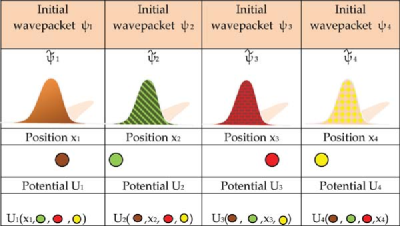
Figure 5: For $4$ interacting particles without exchange interaction, the present algorithm needs $N=4$ single-particle wave functions, $\psi_{a}(x_{a},t)$. The subindex $a$ of the wave function is associated with the potential $U_{a}(x_{a},\vec{x}_{b}[t],t)$ and the initial wave packet. Each wave function $\psi_{a}(x_{a},t)$ determines the $a$-Bohmian trajectories $x_{a}[t]$. See also Color Insert.

For example, for a system of $N=4$ interacting electrons, as depicted in the scheme of Fig. 5, we need to solve $N=4$ Schrödinger-like equations defined by Eq. (105) to find $N=4$ wave functions $\tilde{\psi}_{a}(x_{a},t)$. Many-particle Bohmian trajectories are computed from the Bohmian velocity Eq. (35) using $\tilde{\psi}_{a}(x_{a},t)$ to compute the current and the square modulus. The term $U_{a}(x_{a},\vec{x}_{b}[t],t)$ can be solved from a Poisson equation (if we deal with Coulomb interaction) and it introduces correlations between particles. The initial wave function $\tilde{\psi}_{a}(x_{a},t=0)$ has to be specified. For example, if we assume that the initial wave function is defined in a region of the space where the many-particle wave function is factorizable, we can use $\tilde{\psi}_{a}(x_{a},0)={\psi}_{a}(x_{a},0)$.

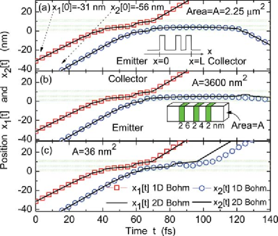
Figure 6: Two-particle interacting Bohmian trajectories in a triple barrier tunneling scenario computed from our 1D approach (symbols) and from exact 2D results (solid line) for three different lateral areas that modify the Coulomb interaction. Reprinted with permission from om.oriolsprl . Copyright 2007 American Physical Society.

We will show now an example of the goodness of this simple approximation. We control the strength of the Coulomb interaction between two electrons by changing the lateral area of a 3D electron device, as described in om.oriolsprl . Figure 6 shows the excellent agreement between exact Bohmian trajectories and those computed with our algorithm. In Fig. 6a, the lateral area is so large that it makes the Coulomb interaction quite negligible. The first electron is transmitted, while the second is reflected. However, as shown in Fig. 6c, the smaller lateral area provides strong Coulomb interaction between the electrons, and the second is finally transmitted because of the presence of the first one in the barrier region.

Certainly, we have used the simplest approximation in Eqs. (103) and (104). Any possible improvement of this approximation will imply an even better agreement between this algorithm and the exact computation.

VI.6.4 Example: Application in interacting many-particle systems with exchange interaction

Now, we generalize the previous result to an arbitrary system with Coulomb and exchange interactions. For simplicity, we will consider only the wave function defined in Eq. (86), that is, only the symmetry of the orbital wave function is considered. A simple Taylor approximation for the terms $G_{a}(x_{a},t)$ and $J_{a}(x_{a},t)$, as we assume in Eq. (103) and Eq. (104), is not valid here. The reason can be easily understood, for example, for a system of (identical) electrons. Due to the Pauli exclusion principle, the modulus of the wave function tends to zero, $R({{x}_{a}},{{\vec{x}}_{b}}[t],t)\to 0$, at every position where ${{x}_{a}}\to{{x}_{k}}[t]$. Thus, the term ${{G}_{a}}({{x}_{a}},{{\vec{x}}_{b}}[t],t)$ has asymptotes at ${{x}_{a}}\to{{x}_{k}}[t]$ that repel other electrons, that is, ${G}_{a}({{x}_{a}},{{\vec{x}}_{b}}[t],t)\to\pm\infty$ at the same particular positions $x_{a}$, invalidating the approximation Eq. (103). For the same reason, ${J}_{a}({{x}_{a}},{{\vec{x}}_{b}}[t],t)\to\pm\infty$.

Here, the strategy is assuming that an antisymmetric wave function, $\Psi(\vec{x},t)$, can be constructed from permutations of a many-particle wave function without any symmetry $\Psi_{\textrm{no-sym}}(\vec{x},t)$:

$$\Psi(\vec{x},{t})=C\sum\limits_{l=1}^{N!}\Psi_{\textrm{no-sym}}(x_{p(l)_{1}},x_{p(l)_{2}},\ldots,x_{p(l)_{N}},t)\;s\left(\vec{p}(l)\right)$$ (107)

The subindex “no-sym” reminds that such wave functions have no spatial symmetric or antisymmetric property. The constant $C$ is a normalization constant that will become irrelevant for the computation of the Bohmian velocity. The sum is over all $N!$ permutations $\vec{p}(l)=\left\{p{{(l)}_{1}},p{{(l)}_{2}},\ldots,p{{(l)}_{N}}\right\}$, and $s\left(\vec{p}(l)\right)=\pm 1$ is the sign of the permutations. Then, each wave function $\Psi_{\textrm{no-sym}}(x_{p(l)_{1}},x_{p(l)_{2}},\ldots,x_{p(l)_{N}},t)$ evaluated at $\vec{x}=\{x_{a},\vec{x}_{b}[t]\}$, can be computed following the previous (no-exchange) algorithm, that is Eqs. (105) and (106). In particular:

$$\Psi_{\textrm{no-sym}}(x_{p(l)_{1}}[t],\ldots,x_{p(l)_{j}},\ldots,x_{p(l)_{N}}[t],t)=\tilde{\psi}_{a,{p}(l)_{j}}(x_{a},t)\exp{(z_{a,\vec{p}(l)}(t))}$$

where the permutation $\vec{p}(l)$ gives $x_{p(l)_{j}}=x_{a}$, that is, ${p(l)_{j}}=a$. Now, we have to use two labels in the subindex of $\tilde{\psi}_{a,h}(x_{a},t)$ to specify the solution of Eq. (105). The first label $a$ accounts for the degree of freedom, that is, the particular trajectory, that we are computing and it also fixes the potential energy $U_{a}(x_{a},\vec{x}_{b}[t],t)$ in Eq. (105). The second label $h$ fixes the initial wave function that we will consider. If the initial many-particle wave function can be defined, in a region without interactions, as:

$$\Psi_{\textrm{no-sym}}(x_{1},\ldots,x_{N},0)=\psi_{1}(x_{1},0)\ldots\psi_{N}(x_{N},0)$$ (109)

then $\tilde{\psi}_{a,{p}(l)_{j}}(x_{a},0)=\psi_{p(l)_{j}}(x_{a},0)$. In other words, identical initial wave functions $\Psi_{i,j}(x_{i},t_{0})=\Psi_{k,j}(x_{k},t_{0})$ can evolve differently when using $U_{i}(x_{i},\vec{x}_{i}[t],t)$ or $U_{k}(x_{k},\vec{x}_{k}[t],t)$.

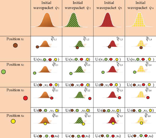
Figure 7: When Coulomb plus exchange interactions are considered, a $4\cdot 4$ matrix of the single-particle wave functions, $\psi_{a,h}(x_{a},t)$ (with $a=1,\ldots,4$ for the potential energies and $j=1,\ldots,4$ for the initial wave packets) is needed to compute (through a Slater determinant) the wave function associated with each Bohmian trajectory. See also Color Insert.

Finally, using Eq. (106), the many-particle wave function $\phi(x_{a},t)=\Psi(x_{a},\vec{x}_{b}[t],{t})$ can be written as:

$$\phi(x_{a},t)=\Psi(x_{a}\vec{x}_{b}[t],{t})=C\sum_{l=1}^{N!}\tilde{\psi}_{a,{p}(l)_{j}}(x_{a},t)\exp{(z_{a,\vec{p}(l)}(t))}\;s\left(\vec{p}(l)\right)$$ (110)

Here, the angles $z_{a,\vec{p}(l)}(t)$ are relevant and cannot be ignored (only a global phase can be ignored). We emphasize that $j$ is selected according to the condition ${p(l)_{j}}=a$, which depends on the index $l$ of the permutations.

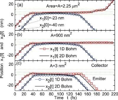
Figure 8: Two-particle Bohmian trajectories with Coulomb and exchange interactions computed from our 1D approach (symbols) and from 2D exact results (solid line) for three lateral areas. Reprinted with permission from om.oriolsprl . Copyright 2007 American Physical Society.

In fact, we can guarantee the expected symmetry of the quantum wave function by defining appropriately the phases. It is quite simple to realize that the following definition of the angles:

$$\exp{(z_{a,\vec{p}(l)}(t))}=\prod^{N}_{k=1,k\neq a}\tilde{\Psi}_{a,p(l)_{k}}(x_{k}[t],t)$$ (111)

accomplishes the symmetry requirements. Finally, putting Eq. (111) into Eq. (110), we obtain the final wave function:

$$\phi(x_{a},t) = C\sum\limits_{l=1}^{N!}{{{\tilde{\Psi}}}_{1,p{{(l)}}_{1}}}({{x}_{1}}[t],t)\ldots{{{\tilde{\Psi}}}_{a,p{{(l)}}_{a}}}({{x}_{a}},t)\ldots{{{\tilde{\Psi}}}_{N,p{{(l)}}_{N}}}{({{x}_{N}}[t],t)s(\vec{p}(l))}$$

This Eq. (LABEL:om.prl_fin) can be simply computed from a (Slater) determinant of the $N\cdot N$ matrix, $\tilde{\psi}_{a,h}(x_{a},t)$ with $a=1,\ldots,4$ and $j=1,\ldots,4$ for the initial wave packets, which are defined in Fig. 7.

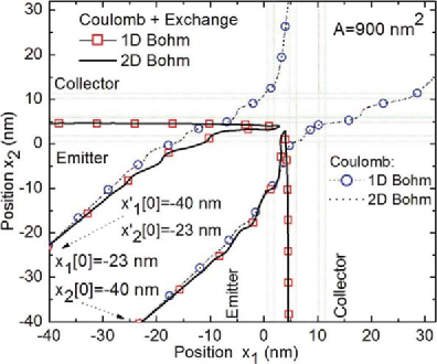
Figure 9: Two-particle Bohmian trajectories with Coulomb and exchange interactions computed from our 1D approach (symbols) and from 2D exact results (solid line) when initial positions are interchanged. Reprinted with permission from om.oriolsprl . Copyright 2007 American Physical Society.

The reader can wonder why we need $N^{2}$ different wave functions and not $N!$. The reason is because the term $U_{a}(x_{a},\vec{x}_{b}[t],t)$ in Eq. (105) does not change when we interchange the positions of two of the trajectories in $\vec{x}_{b}[t]$ (only the interchange between $x_{a}[t]$ and a trajectory of $\vec{x}_{b}[t]$ becomes relevant). Figure 8 shows the excellent agreement between the exact Bohmian trajectories and those computed from this second algorithm. See details in om.oriolsprl .

In order to clarify the meaning of indistinguishable particles in the Bohmian language, in Fig. 9, we simulate Bohmian trajectories with the initial positions and with interchanged initial positions. By our own construction of the wave function of Eq. (LABEL:om.prl_fin), the velocity has symmetry when we interchange particles, as discussed in Sec. VI.4. Therefore, although we can distinguish each electron by its own trajectories, one cannot discern between them in the final observable results. For example, the number of events where the first trajectory is transmitted and the other reflected is exactly identical to the events where the first is reflected, while the second is transmitted. On the contrary, as seen in Fig. 9, this symmetry is broken without the exchange interaction algorithm.

VII Bohmian Explanation of the Measurement Process

The Bohmian explanation of a quantum measurement process is, perhaps, the most attractive (and also ignored) feature of the Bohmian explanation of the quantum nature om.bell1990 ; om.Durrllibre ; om.Goldsteinobserver ; om.Bell1966 ; om.bomhhiley1993 ; om.reviewabc ; om.llibreph . Let us start by noting that Bell disliked the word “measurement” om.bell1990 . He preferred the word “experiment” because “when it is said that something is measured it is difficult not to think of the result as referring to some pre-existing property of the object in question.” On the contrary, in an experiment, it is natural to think that everything can change (time-evolve), because of the interactions. Once we admit that the system itself can be modified during the measurement, we can easily understand that the output of a measurement depends on the duration and strength of the measurement process, on the previous measurements, etc.

VII.1 The measurement problem

We have previously talked about the so-called measurement problemom.Dieter ; om.maudlin ; om.bohm66 but, what is in fact this measurement problem? It is a problem related to the application of the superposition law in quantum systems. Quantum states of a particle are represented by vectors in a Hilbert space such that linear combinations of them, for example a superposition of macroscopically distinguishable states, also correspond to valid states of the Hilbert space. However, such superposition of states is not always compatible with measurements om.bohm66 ; om.nikolic . The measurement problem can be formulated as the impossibility for a physical quantum theory (in empirical agreement with experiments) to simultaneously satisfy the following three assumptions om.maudlin .

1. The wave function always evolves deterministically according to the linear and unitary Schrödinger equation.

2. A measurement always finds the physical system in a localized state, not in a superposition of macroscopically distinguishable states.

3. The wave function is a complete description of a quantum system.

A theory that includes all three assumptions is not empirically compatible with the experimental results. Different physical theories are developed depending on which assumption is ignored om.herbert . The measurement problem appears because none of the proposed solutions fully satisfies the whole scientific community.

The first type of solutions argues that the unitary and linear evolution of the Schrödinger equation is not always valid (such solutions ignore the (1) assumption). For instance, in the instantaneous collapse theories om.bassi13 (like the GRW interpretation om.ghirardi86 ), a new stochastic equation is used that breaks the superposition principle at the macroscopic level, while still keeping it at the microscopic one om.bassi13 . Another possibility is substituting the linear Schrödinger equation by a non-linear collapse law only when a measurement is performed om.bohr20 . This is the well-known orthodox or Copenhagen solution. The dissatisfaction with the Copenhagen solution is that the theory does not clearly specify when, in which circumstances, the linear or non-linear equation has to be used.

A second type of solution ignores the (2) assumption that a measurement always finds the physical system in a localized state. One then concludes that there are different worlds where different states of the superposition are found. This is the many worlds solution om.Everett57 ; om.wallace12 in which the famous Schrödinger’s cat is found alive in one world and dead in another.

There is a final kind of solutions that assumes that the wave function alone does not provide a complete description of the quantum state, that is, it ignores the (3) assumption and includes additional elements (hidden variables) in the theory. The most spread of these approaches is Bohmian mechanics explained in this book. In a spatial superposition of two disjoint states for a single-particle system, only the one whose support contains the position of the particle becomes relevant for the dynamics. Notice that, in Bohmian mechanics, it is not mandatory to define which interactions are considered a measurement and which are not. All interactions (implying a measurement or not) are treated identically.

Let us discuss in more detail the differences between an orthodox and a Bohmian measurement. As we have already explained, in Bohmian mechanics, the evolution of the wave function is determined by the Schrödinger equation (when the appropriate Hamiltonian is used). This is not true for the orthodox formulation of the measurement because one linear equation (the Schrödinger equation) is used for non-measuring interactions, while a different non-linear equation (the collapse law) is needed to tackle measuring interactions.

VII.1.1 The orthodox measurement process

In any attempt to study a quantum system, one usually separates the quantum system itself and the rest. The separation is arbitrary, but mandatory in any practical computation since it is impossible to deal with all degrees of freedom of the system and the rest. This separation is also typical in the modeling of a quantum measurement. Let us notice that, in principle, the origin of the separation between the quantum system and the measuring apparatus is technical; it is not a direct consequence of the quantum theory that we select to describe the quantum world. However, it is true that, because of the ontology of the Copenhagen theory, the measurement process is explained by a proper separation between the system and the measuring apparatus (see Fig. 10b), while the Bohmian theory tends to consider system and apparatus altogether (see Fig. 10a).

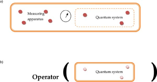
Figure 10: (a) The Bohmian measurement is better explained by assuming that the quantum system and the measuring apparatus are two interacting systems. (b) The typical orthodox measurement is better explained by assuming that only the quantum system is explicitly simulated, while the measuring apparatus is substituted by a proper operator acting on the wave function of the system.

The typical orthodox prediction of some experimental property of the quantum system is described through the use of a proper operator $\hat{G}$ whose eigenvalues give the possible outcomes of the measurement. When we measure a particular eigenvalue, the initial wave function is transformed into an eigenfunction of the operator. This is the so-called von Neumman (or projective) measurement. Thus, the time evolution of the wave function of a quantum system is governed by two (quite) different laws:

1. The first dynamical evolution is given by the Schrödinger equation. This dynamical law is deterministic in the sense that the final wave function of the quantum system is perfectly determined when we know the initial wave function and the Hamiltonian of the quantum system.

2. The second dynamical law is called the collapse of the wave function. The collapse is a process that occurs when the wave function interacts with a measuring apparatus. The initial wave function before the measurement is substituted by one of the eigenstates of the particular operator $\hat{G}$​. Contrarily to the dynamical law given by the Schrödinger equation, the collapse is not deterministic, since the final wave function is randomly selected among the operator’s eigenstates.

The duality in the equation of motions (linear or non-linear) of a quantum system in the orthodox interpretation is certainly a persistent controversial issue. There are many scientist unsatisfied with this solution of the measurement problem om.bell1990 . As repeatedly stressed by Bell, the orthodox theory is unprofessional because it does not explain with total accuracy which parts of the entire quantum system form the measuring apparatus and which the quantum system itself. It is even not clear if the measuring apparatus needs some kind of human activity (with a PhD? om.bell1990 ) to be accepted as a proper measuring apparatus. The problematical way in which measurement is treated in the orthodox formulation has been stressed by Bell om.Bell1987 :

The concept of “measurement” becomes so fuzzy on reflection that it is quite surprising to have it appearing in physical theory at the most fundamental level. Less surprising perhaps is that mathematicians, who need only simple axioms about otherwise undefined objects, have been able to write extensive works on quantum measurement theory-which experimental physicists do not find it necessary to read. […] Does not any analysis of measurement require concepts more fundamental than measurement? And should not the fundamental theory be about these more fundamental concepts?

In short, Bell argued that the separation between the quantum system and the measuring apparatus in Fig. 10b is arbitrary. For practical computations, the encapsulation of the rest of the world (except the quantum system) into a mathematical entity called an operator, $\hat{G}$​, is a very clever trick that allows for straightforward calculations of the results of quantum measurements om.Durrnaive ; om.goldstein without considering the rest of the world. However, conceptually, the role played by the operator $\hat{G}$ as a fundamental part of the orthodox theory is at the origin of the criticism against the orthodox solution of the measurement problem.

The reader can argue that, since we have said that the separation between the system and the rest is always arbitrary, one can always enlarge what we consider as a system (see Fig. 10a) also in the orthodox formulation of the measurement. This would not solve the measurement problem in the orthodox formulation. Certainly, we can enlarge the system in the orthodox quantum formulation of the measurement process by including as a system part of what was defined previously as an apparatus. The degrees of freedom of the new system will interact with the degrees of freedom of the old system through a linear equation of motion (Schrödinger equation). Therefore, we will always need something external to the enlarged system (some new operator $\hat{G}$​) to provide the collapse of the wave function of the enlarged system.

VII.1.2 The Bohmian measurement process

In Bohmian theory, the measurement process is treated just as any other quantum process of interacting particles and the previous measurement difficulties of the orthodox interpretation simply disappear. At least, from a conceptual point of view. There is no need to introduce operators om.Durrnaive ; om.Durrllibre ; om.goldstein ; om.reviewabc ; om.llibreph . Here, the entire quantum system is described by a many-particle trajectory plus a many-particle wave function (rather than a wave function alone). The wave function and the trajectory are both associated with the entire system, that is, the quantum system plus the measuring apparatus. Then, there is one dynamical law for the evolution of the wave function and another for the evolution of the trajectory:

1. The Schrödinger equation (with the appropriate Hamiltonian of the quantum system plus the measuring apparatus) determines the time evolution of the wave function independently of whether a measurement process takes place or not.

2. The time evolution of the particle is determined by the time integration of the Bohmian velocity independently of whether a measurement process takes place or not.

For example, imagine that some kind of pointer indicates the measured quantity; then, the particles (degrees of freedom) that form the pointer must be present in the Hamiltonian. In this sense, in Bohmian mechanics, a physical quantum system must be described by a many-particle Hamiltonian. Once the Bohmian trajectories associated with the positions of the pointer are known, the value of the measurement is already predicted. We just need knowledge of the positions of the pointer particles. Again, Bell provided us with one of his didactic sentences om.Bell1987 :

In physics the only observations we must consider are position observations, if only the positions of instrument pointers. It is a great merit of the de Broglie–Bohm picture to force us to consider this fact. If you make axioms, rather than definitions and theorems, about the “measurement” of anything else, then you commit redundancy and risk inconsistency.

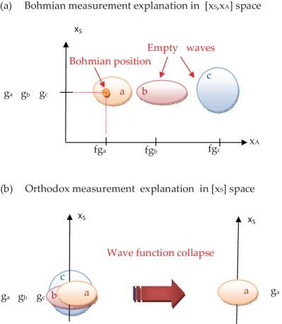
Figure 11: (a) Bohmian measurement in the $[x_{S},x_{A}]$ space: From the nonoverlapping many-particle (system + apparatus) wave function, only the $g_{a}$ part of the wave function where the trajectory is present is needed to compute the evolution of the Bohmian system. (b) Orthodox measurement in the $[x_{S}]$ space: The (system) wave function collapses into the $g_{a}$ part when the measurement takes place. See also Color Insert.

Therefore, a proper modeling of a Bohmian measurement just needs the explicit consideration of the degrees of freedom of the pointer in the many-particle wave function and many-particle Bohmian trajectories that define the entire system. See Fig. 11. In particular, we have to introduce into the Hamiltonian the interaction of the particles of the pointer with the rest of the particles of the system. The back reaction of the measurement process on the wave function is trivially considered. Certainly, a Hamiltonian with or without the measuring apparatus will provide a different evolution of the quantum system wave function. For this reason, Bell preferred the word “experiment” instead of “measurement.”

The Bohmian and the orthodox explanations of a measurement produce the same probabilistic predictions. However, the mathematical implementation of the equations of motion in each case is quite different. The orthodox quantum theory requires an operator to describe the effect of the measuring apparatus, but this operator is not needed in the Bohmian explanation.

To be fair, the simplicity of the Bohmian measurement is true at the conceptual level explained above. However, any practical attempt to directly implement the Bohmian protocol will have to face with the many body problem discussed in Sec. VI.1. A pointer in a measuring apparatus is a macroscopic object with a number of particles on the order of Avogadro’s number ($\approx 10^{23}$ particles). Can we simulate such large number of particles and look at the “position of the instrument pointers” to get the measured valued as suggested by Bell? From a practical point of view, the answer is no because of the computational burden. Approximations reducing the simulated degrees of freedom, implying the artificial separation of the whole Bohmian system (as depicted in Fig. 10b) into systems plus apparatus (as depicted in Fig. 10a), will be mandatory.

VII.2 Theory of the Bohmian measurement process

Now, we provide a mathematical demonstration of the equivalence between orthodox and Bohmian measurements for a typical ensemble over identical experiments. In the standard interpretation of quantum theory, the von Neumann (projective) measurement process is defined in a particular quantum region, which is defined through the degrees of freedom $\vec{x}_{S}$. See Fig. 11b. The state of the quantum system in this particular region is determined through the wave function $\psi_{S}(\vec{x}_{S},t)$. The process of measuring a particular magnitude is mathematically defined through an operator, for example $\hat{G}$, acting on the wave function. The possible outcomes of the measurement process correspond to one of the possible eigenvalues $g$ of this operator that satisfy the equation $\hat{G}\psi_{g}(\vec{x}_{S})=g\psi_{g}(\vec{x}_{S})$ with $\psi_{g}(\vec{x}_{S})$, an eigenvector of this operator. The set $\psi_{g}(\vec{x}_{S})$ forms an orthonormal basis of the Hilbert space of the quantum system so that the arbitrary initial wave function can be written as:

$$\psi_{S}(\vec{x}_{S},t)=\sum_{g}c_{g}(t)\psi_{g}(\vec{x}_{S})$$ (113)

with $c_{g}(t)=\int\psi_{S}(\vec{x}_{S},t)\psi_{g}^{*}(\vec{x}_{S})$ a complex value with the only restriction $\sum_{g}|c_{g}(t)|^{2}=1$ in order to ensure that $\psi_{S}(\vec{x}_{S},t)$ is well normalized. When measuring the eigenvalue $g_{a}$ the total wave function $\psi_{S}(\vec{x}_{S},t)$ collapses into $\psi_{g_{a}}(\vec{x}_{S})$. Then, the probability of obtaining $g_{a}$ in the measuring apparatus is just $P_{g_{a}}=|c_{g_{a}}(t)|^{2}$. To avoid unnecessary complications, hereafter, we have assumed that the basis $\psi_{g}(\vec{x}_{S})$ has no degeneracy.

In order to understand how this (von Neumann) measurement can be described by means of Bohmian mechanics, we use the Schrödinger equation plus a trajectory, defined both in the enlarged configuration space that includes the quantum system and the measuring apparatus. There is no privileged status for the observer, that is, the measuring apparatus, over the quantum system. This is the reason why some authors describe Bohmian theory under the title of “quantum mechanics without observers” om.Goldsteinobserver .

Surprisingly, this idea was, somehow, anticipated in the book Quantum Theory, published in 1951 om.bohmbook , by Bohm. Although in this book Bohm followed an orthodox presentation of quantum mechanics, he also provided a detailed and conceptually intricate treatment of the measurement process in chapter 22. First, Bohm demanded in unequivocal terms a quantum theoretical treatment of the entire process of measurement within the Schrödinger equation. In particular, he argued that a good measuring apparatus will force the wave function to decouple into several nonoverlapping wave packets. Each one of these wave packets can be associated to one particular value of the measurement process. Second, he supplemented his measurement process by adding some obscure discussion about decoherence where only one of the several wave packets survives (as we mentioned at the end of Sec. VII.1.1, even after enlarging the system, one has to invoke somehow the collapse of the wave function). After 1951, when Bohm presented his “hidden variables” theory om.bohm1952a ; om.bohm1952b , he kept the first part of his previous explanation of the measurement process and then provided a simple explanation about the final selection of the available wave packets: the selected wave packet is the one that contains the trajectory, see Fig. 1.10(a).

Our mathematical demonstration on how Bohmian mechanics explains the (von Neumann) measurement follows om.Holand1993 ; om.bomhhiley1993 ; om.Durrnaive ; om.Durrllibre ; om.llibreph . In order to be able to define the measurement process in the Bohmian formalism, apart from the degrees of freedom $\vec{x}_{S}$, we need the degrees of freedom of the positions $\vec{x}_{A}$ of the pointer belonging to a measuring apparatus. Thus, we define a total wave function $\Phi_{T}(\vec{x}_{S},\vec{x}_{A},t)$ in a larger configuration space that includes the quantum region plus the measuring region, $\{\vec{x}_{S},\vec{x}_{A}\}$. According to the Bohmian postulates, we do also select a trajectory $\{\vec{x}_{S}[t],\vec{x}_{A}[t]\}$ in this larger configuration space. The (Bohmian) time evolution of the total wave function and the total trajectory is what we need to explain the (von Neumann) measurement process described earlier .

There are some necessary conditions that the time-evolution of the entire Bohmian system has to satisfy to say that a measuring apparatus is able to correctly determine the eigenvalues $g$. First, the pointer positions $\vec{x}_{A}[t]$ of such an apparatus have to be restricted to a particular region, $\vec{x}_{A}[t]\in S_{g_{1}}$, every time that the quantum system is in the eigenstate $\psi_{g_{1}}(\vec{x}_{S})$. Let us define $\Phi_{g_{1}}(\vec{x}_{S},\vec{x}_{A},t)$ as the total wave function that fits with the property that any experiment whose quantum system is described by $\psi_{g_{1}}(\vec{x}_{S})$ implies that the pointer points in the particular region, $\vec{x}_{A}[t]\in S_{g_{1}}$. A second necessary condition for a good measuring apparatus of the eigenvalue $g$ is that $S_{g1}\cap S_{g2}=0$ when we measure. We have defined the restricted region allowed by the pointer positions associated with a second eigenstate, $\psi_{g_{2}}(\vec{x}_{S})$, as $\vec{x}_{A}[t]\in S_{g_{2}}$. This implies that the states $\Phi_{g_{1}}(\vec{x}_{S},\vec{x}_{A},t)$ and $\Phi_{g_{2}}(\vec{x}_{S},\vec{x}_{A},t)$ do not overlap in the larger configuration space during the measurement.

Since the eigenstates $\psi_{g}(\vec{x}_{S})$ form a complete basis, we can decomposed any function, and in particular each $\Phi_{g}(\vec{x}_{S},\vec{x}_{A},t)$, into the following sum:

$$\Phi_{g}(\vec{x}_{S},\vec{x}_{A},t)=\sum_{g^{\prime}}f_{g^{\prime}}(\vec{x}_{A},t)\;\psi_{g^{\prime}}(\vec{x}_{S}),$$ (114)

with $f_{g}(\vec{x}_{A},t)=\int\Phi_{g}(\vec{x}_{S},\vec{x}_{A},t)\psi^{*}_{g}(\vec{x}_{S})d\vec{x}_{S}$. However, from our previous discussion about the properties of a “good” von Neumann measurement apparatus, $\Phi_{g}(\vec{x}_{S},\vec{x}_{A},t)$ cannot be a sum over different eigenstates $\psi_{g}(\vec{x}_{S})$ in Eq. (114) because then the measuring apparatus would provide the same pointer position $\vec{x}_{A}[t]\in S_{g}$ for different eigenstates. Thus, during the time of the measurement, the only good decomposition for $\Phi_{g}(\vec{x}_{S},\vec{x}_{A},t)$ is:

$$\Phi_{g}(\vec{x}_{S},\vec{x}_{A},t)=f_{g}(\vec{x}_{A},t)\;\psi_{g}(\vec{x}_{S})$$ (115)

We emphasize that $f_{g}(\vec{x}_{A},t)$ is a normalized function because $\Phi_{g}(\vec{x}_{S},\vec{x}_{A},t)$ and $\psi_{g}(\vec{x}_{S})$ are also normalized functions in their respective configurations spaces. By its own construction, $f_{g_{1}}(\vec{x}_{A},t)\cap f_{g_{2}}(\vec{x}_{A},t)=0$ during the measuring time. Thus, even if $\psi_{g_{1}}(\vec{x}_{S})$ and $\psi_{g_{2}}(\vec{x}_{S})$ overlap, the states $\Phi_{g_{1}}(\vec{x}_{S},\vec{x}_{A},t)$ and $\Phi_{g_{1}}(\vec{x}_{S},\vec{x}_{A},t)$ do not overlap in the larger configuration space. See Fig. 11a. Thus, we can ensure that a general function in the quantum system, Eq. (113), can be rewritten in the whole, that is, quantum plus measuring, configuration space associated to a good measuring apparatus as:

$$\Phi_{T}(\vec{x}_{S},\vec{x}_{A},t)=\sum_{g}c_{g}(t)\;\;f_{g}(\vec{x}_{A},t)\;\psi_{g}(\vec{x}_{S})$$ (116)

In summary, during the time of measurement, the only total wave functions that can live in the entire quantum system that includes a good (in this case a projective or Von-Neumann type) measuring apparatus of the eigenvalues $g$ are the ones written in Eq. (116). An example of such wave functions is depicted in Fig. 11a. It is important to notice that Eq. (116) implies no restriction on the wave function $\psi_{S}(\vec{x}_{S},t)$ but only on the total wave function $\Phi_{T}(\vec{x}_{S},\vec{x}_{A},t)$. If these restrictions are not respected, we can find other types of total wave functions in the configuration space $\{\vec{x}_{S},\vec{x}_{A}\}$, but they would be incompatible with stating that we have an apparatus that is able to measure the eigenavalue $g$ with certainty at time $t$.

After this discussion, we can show quite trivially how the von Neumann measurement is exactly reproduced with Bohmian mechanics. As we have mentioned, apart from the wave function in Eq. (116), we have to select an initial trajectory $\{\vec{x}_{S}[0],\vec{x}_{A}[0]\}$. Such a trajectory will evolve with the total wave function, and during the measurement, the particle trajectory $\{\vec{x}_{S}[t],\vec{x}_{A}[t]\}$ will be situated in only one of the nonoverlapping wave packets of Eq. (116), for example $f_{g_{a}}(\vec{x}_{A},t)\psi_{g_{a}}(\vec{x}_{S})$ as depicted in Fig. 11a. Thus, the pointer positions will be situated in $\vec{x}_{A}[t]\in S_{g_{a}}$ and we will conclude with certainty that the eigenvalue of the quantum system is $g_{a}$. In addition, the subsequent evolution of this trajectory can be computed from $f_{g_{a}}(\vec{x}_{A},t)\psi_{g_{a}}(\vec{x}_{S})$ alone. In other words, we do not need the entire wave function Eq. (116) because the particle velocity can be computed from $f_{g_{a}}(\vec{x}_{A},t)\psi_{g_{a}}(\vec{x}_{S})$. The rest of circles of Fig. 11a are empty waves that do not overlap with $f_{g_{a}}(\vec{x}_{A},t)\psi_{g_{a}}(\vec{x}_{S})$ so that they have no effect on the velocity of the Bohmian particle. This is the simple explanation of how the complicated orthodox collapse is interpreted within Bohmian mechanics. This discussion is depicted in Fig. 11

We have mentioned before that the von Neumann measurement predicts that the probability of finding $g_{a}$ is $P_{g_{a}}=|c_{g_{a}}(t)|^{2}$. We can easily recover this result from our Bohmian picture. This probability is obtained after the repetition of the same experiment, with the same $\Phi_{T}(\vec{x}_{S},\vec{x}_{A},t)$, many times. The second (quantum equilibrium) postulate of Bohmian mechanics (see Sec. VI.5) ensures that the modulus of the wave function will be reproduced by the trajectories when we repeat the same experiment many times. Then, the probability of finding the eigenvalue $g_{a}$, that is, the eigenstate $\psi_{g_{a}}(\vec{x}_{S})$, is just:

$$P_{g_{a}} = \frac{\int\int|c_{g_{a}}(t)f_{g_{a}}(\vec{x}_{A},t)\psi_{g_{a}}(\vec{x}_{S})|^{2}d\vec{x}_{S}d\vec{x}_{A}}{\int\int\sum_{g}|c_{g}(t)f_{g}(\vec{x}_{A},t)\psi_{g}(\vec{x}_{S})|^{2}d\vec{x}_{S}d\vec{x}_{A}}=\frac{|c_{g_{a}}(t)|^{2}}{\sum_{g}|c_{g}(t)|^{2}}=|c_{g_{a}}(t)|^{2}$$ (117)

where we have explicitly used the condition that the each $\Phi_{g_{1}}(\vec{x}_{S},\vec{x}_{A},t)$ does not overlap with the others for the computation of the modulus of the total wave function, $|\Phi_{T}(\vec{x}_{S},\vec{x}_{A},t)|^{2}$, in the denominator. Additionally, we use $\int|\psi_{g}(\vec{x}_{S})|^{2}d\vec{x}_{S}=1$, $\int|f_{g}(\vec{x}_{A},t)|^{2}d\vec{x}_{A}=1$, and $\sum_{g}|c_{g}(t)|^{2}=1$. Thus, the same probabilistic predictions are obtained from Bohmian and orthodox quantum formulations when a von Neumann measurement is performed.

We want to enlarge the explanation of the role played by the empty waves belonging to the wave packet of Eq. (116), which do not contain the particle. In principle, one can argue that such empty waves can evolve and, in later times, overlap with the original wave that contains the particle. If we are interested in doing subsequent (i.e., two times) quantum measurements, a good measuring apparatus has to avoid these “spurious” overlaps. This can be understood as an additional condition for qualifying our measuring apparatus as a good apparatus. In the examples of the subsequent subsections VII.2.1 and VII.2.2, we will realize that the assumption of nonoverlapping between empty and full waves can be very reasonable in many practical implementations of the measuring apparatus. In fact, in a real system with a very large number of particles associated to the apparatus (or the environment), the probability that such overlap occurs in the configuration space of all the particles is almost null. See a discussion on page 79 in Ref. om.bomhhiley1993 . If the empty wave packets later coincide (by putting some reflected mirrors for example), then, the apparatus described above would not be a good apparatus to measure eigenvalues. On the contrary, this apparatus (with the mirrors) would be a very interesting/enlightening design to test quantum interference effects with waves and particles. The double-slit experiment is the most famous example of interference effects between empty and full wave packets.

Finally, let us mention that we have only considered von Neumann (i.e., projective) measurements. Other types of measurements are also possible, which do not collapse into an eigenstate (for example, the generalized or weak measurements). Obviously, such generalized measurements can also be explained within Bohmian mechanics with an extension of the simple ideas for projective measurements discussed here om.bomhhiley1993 ; om.Durrnaive ; om.Durrllibre .

VII.2.1 Example: Bohmian measurement of the momentum

Let us explain the momentum measurement of the stationary state of an electron initially in an energy eigenstate of a square well of size $L$. For example, $\psi_{n}(x)=C\;\sin(n\pi x/L)$ within the well and zero elsewhere, $C$ being the normalization constant and $n$ an integer (denoting the vibrational state). Since the wave function is real, we obtain $p=\partial S(x)/\partial x=0$. Thus, the Bohmian particle is at rest, meaning that its velocity and kinetic energy are zero. However, we know that for a high enough value of $n$, the previous wave function $\psi(x)$ can be roughly approximated by a sum of two momentum eigenstates with eigenvalues $\pm n\hbar/L$. Therefore, when we do a (Copenhagen) momentum measurement, we will obtain an outcome $\pm n\hbar/L$ and the previous wave function will collapse into one of the two momentum eigenstates.

We have shown that the Bohmian measurement has to provide the same eigenvalues and eigenstates. How? The answer is that according to the Bohmian measurement, we have to specify in detail how the measurement process develops; which is the Hamiltonian that provokes the measurement.

A measurement of the momentum, for example, can be undertaken by removing the walls that form the well and detecting the electron somewhere in a screen far from the initial walls. The time interval between removing the walls and detecting the particles will allow us a computation of the “electron velocity.” The time-dependent process of removing the walls will imply that the stationary wave function will evolve into two time-dependent wave packets moving on opposite directions, which will become completely separated in space. The particle will end in one wave packet or the other with a momentum very close to $\pm n\hbar/L$, the sign depending on which wave packet the initial position of the particle enters om.bohm1952b . Finally, the electron will be detected far from the walls after the appropriate interval of time. For this particular experiment, we are sure that the empty wave will not affect the wave that carries the particle. As mentioned earlier, the relevant point is that we have been able to measure the same eigenstates and eigenvalues predicted by the orthodox interpretation without invoking the collapse of the wave function as a fundamental law.

In order to understand the Bohmian explanation of this experiment, it is important to discuss the roles played by the kinetic and quantum potentials. The initial Bohmian kinetic energy is zero, while the initial quantum potential is $Q(x,t)=(n\hbar/L)^{2}/(2m)$ for the initial state $\psi(x)=C\;sin(n\pi x/L)$. On the contrary, the final energy of the system appears in the form of kinetic energy of electrons $(n\hbar/L)^{2}/(2m)$, while the final quantum potential from Eq. (6) is negligible $Q(x,t)\sim 0$. See problem 10.

The reader will realize that we have not follow all the indications of the previous section. In principle, for a formal Bohmian discussion of measurement, we would have to discuss the wave function and particles of the whole quantum plus measuring apparatus system. However, in this section we have avoided the wave function and trajectory related to the measuring apparatus. In this example, the screen is the measuring apparatus of the position of the system’s particle. The part of the measuring process involving the screen has not been explicitly described in our example (we could obviously explain why a proper coupling of the degrees of freedom of the system and the screen will imply that after impinging with the screen, the system wave function becomes a wave packet highly localized around the position of the measurement, but we have not done it because it is quite obvious).

This example clearly shows that what we get from a measurement depends on the measurement itself. We have explained an experiment to measure the velocity of the particle. In fact, the Bohmian particle was at rest (with zero velocity) before we start the measurement. However, because of the type of measurement that we have designed, the Bohmian particle acquires a non-zero velocity. What we get from the measurement is exactly this non-zero value of the velocity, but this is not the pre-existing velocity of the particle before the measurement. Contrarily to a classical measurement, in the quantum world, in general, we cannot get information of a quantum system from a measurement without providing some type of perturbation on it. This property of quantum phenomena is named contextuality.

VII.2.2 Example: Sequential Bohmian measurement of the transmitted and reflected particles

We provide another didactic example of how Bohmian mechanics explains sequential measurements. The wave packets in Fig. 12 represent the solution of the (unitary) Schrödinger equation for a wave packet incident upon a tunneling barrier, at three different times. The initial wave packet (with norm equal to one) is divided into a transmitted plus a reflected wave packet. According to the Copenhagen interpretation, when the system is measured at time $t_{1}$, a nonunitary evolution appears in the wave function. Thus, randomly, for example the reflected wave packet disappears. Only the transmitted wave packet describes the electron at time $t_{1}$. Then, when the system is measured again at $t_{2}$, the electron is only represented by the transmitted wave packet.

Alternatively, the same evolution can be explained with Bohmian mechanics. The initial position of the Bohmian trajectory is selected according to the quantum equilibrium hypothesis at the initial time $t_{0}$. Let us assume that we select an initial position that corresponds to a trajectory that is finally transmitted. Then, at times $t_{1}$ and $t_{2}$, the evolution of the trajectory is only determined by the transmitted wave packet because the reflected wave packet is an “empty wave” that has no effect on the evolution of the trajectory. Here, we have implicitly assumed that the eigenstates of the measuring apparatus are transmitted wave packets for positive currents, and reflected ones for negative currents.

As expected, the probability of measuring, first, the particle as being transmitted at time $t_{1}$ and measuring, after, the same particle as being reflected at time $t_{2}$ is zero either with orthodox or Bohmian mechanics.

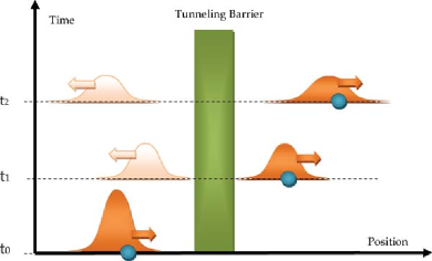
Figure 12: Schematic explanation of the ability of Bohmian mechanics to discuss the unitary and nonunitary evolution of a wave packet incident upon a tunneling barrier for three different times $t_{0}<t_{1}<t_{2}$.

Again, the reader can argue that we have not enlarged the system including the measuring apparatus. Next, we provide a more formal description of the Bohmian measurement of the charge for a tunneling electron including the quantum system plus the measuring apparatus. The quantum system is defined by an electron labeled as $x_{1}[t]$ impinging on a tunneling barrier. Behind the barrier there is a measuring device named the “transmitted charge detector” and modeled as a single degree of freedom $x_{2}[t]$, which can detect the successful transmission of an electron. The dynamic of the system plus apparatus includes, first, an interaction of the electron with the potential barrier and, subsequently, an interaction with the transmitted charge detector. It is important to stress that both interactions are regarded at the very same level within Bohmian mechanics. The measurement interaction introduces a channelization of the wave function in the configuration space such that the desired property of the quantum system (here, whether the electron is reflected or transmitted) can be read off from the final position $x_{2}[t]$ of a particle, which plays the role of the pointer of the apparatus. The interaction between the electron and the pointer can be modeled as:

$$H_{int}=\lambda Q(x_{1})P_{x_{2}}=-i\hbar\lambda Q(x_{1})\frac{\partial}{\partial x_{2}},$$ (118)

where $P_{x_{2}}=-i\hbar\partial/\partial x_{2}$ is the momentum operator of the detector and $\lambda=50\;nm/ps$ is the interaction constant. $Q(x_{1})$ is a function that is equal to zero when the electron is outside the detector, ($x_{1}<75\;nm$ in Fig. 13), and is equal to one when the particle is inside the detector ($x_{1}>75\;nm$). In Fig. 13 the region in the configuration space in which $Q(x_{1})$ is different from zero is represented by a rectangle in the right of the figure. The many-particle Schrödinger equation reads

$$i\hbar\frac{\partial\Psi(x_{1},x_{2},t)}{\partial t}=\Big{(}-\frac{\hbar^{2}}{2m}\frac{\partial^{2}}{\partial x_{1}^{2}}-\frac{\hbar^{2}}{2M}\frac{\partial^{2}}{\partial x_{2}^{2}}+U(x_{1})-i\hbar\lambda Q(x_{1})\frac{\partial}{\partial x_{2}}\Big{)}\Psi(x_{1},x_{2},t),$$

(119)

where $m$ is the effective mass of the electron, $M$ is the mass of the apparatus pointer and $U(x_{1})$ is the external potential energy barrier seen as a vertical line in the middled of Fig. 13.

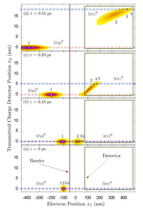
Figure 13: Time evolution of the squared modulus of $\Psi(x_{1},x_{2},t)$ at four different times. The configuration space region where the transmitted charge detector is present is indicated by a rectangle and the barrier by a solid line. The $+$ line indicates the squared modulus of the conditional wave function $|\psi_{R}|^{2}=|\Psi(x_{1},x_{2}^{\alpha=1}[t],t)|^{2}$, while the $\odot$ line corresponds to $|\psi_{T}|^{2}=|\Psi(x_{1},x_{2}^{\alpha=3}[t],t)|^{2}$. Four trajectories $\{x_{1}^{\alpha}[t],x_{2}^{\alpha}[t]\}$ with different initial positions are presented with $[]$, $*$, $\times$ and $+$. The actual detector position associated with the reflected trajectory ($+$) with $\alpha=1$ does not move because there is no interaction between this trajectory and the detector. Reprinted with permission from om.albareda . Copyright 2013 Springer Nature.

The main feature of a transmitted charge detector is that the center of mass of the wave function in the $x_{2}$ direction has to move if the electron is transmitted and it has to be at rest if the electron is reflected. We solve Eq. (119) numerically considering as initial wave function the products of two gaussian wave packets, i.e. $\Psi(x_{1},x_{2},0)=\psi(x_{1},0)\phi(x_{2},0)$. All details of this simulation can be found in Ref. om.albareda ; om.2marian . In particular we are considering $M=75000\;m$. In Fig. 13 the numerical solution of the squared modulus of $\Psi(x_{1},x_{2},t)$ is plotted at four different times. At the initial time $t=0$, Fig. 13 (a), the entire wave function is at the left of the barrier. At a later time $t_{0}$ the wave function has split up into reflected and transmitted parts due to the barrier, see Fig. 13 (b). Then, because the electron has not yet arrived at the transmitted charge detector, the wave function has the following form:

$$\Psi(x_{1},x_{2},t_{0})=\left[\psi_{T}(x_{1},t_{0})+\psi_{R}(x_{1},t_{0})\right]\phi(x_{2},t_{0}).$$ (120)

After that, Figs. 13 (c) and (d), the interaction of the detector with the transmitted part of the wave function appears. For time $t>t_{0}$ the transmitted part of the wave function is shifted up in the $x_{2}$ direction while the reflected part does not move. The interaction with the apparatus thus produces two channels in the configuration space, one corresponding to the electron being transmitted and the other corresponding to the electron being reflected, getting an entangled superposition among the electron and the apparatus.

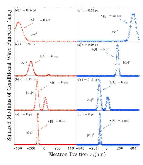
Figure 14: The $+$ line in (a), (b), (c) and (d) is the time evolution of the squared modulus of the conditional wave function associated to the trajectory $\alpha=1$ in Fig. 13, i.e. $\psi_{R}=|\Psi(x_{1},x_{2}^{\alpha=1}[t],t)|$. The $\odot$ line in (e), (f), (g) and (h) is the squared modulus of the conditional wave function associated to the trajectory $\alpha=3$ in Fig. 13. i.e. $\psi_{T}=|\Psi(x_{1},x_{2}^{\alpha=3}[t],t)|$. The actual detector position $x_{2}[t]$ is plotted at each time in order to compare these results with those in Fig. 13. Reprinted with permission from om.albareda . Copyright 2013 Springer Nature.

In Fig. 13 we also plot the actual positions of the system and detector $\{x_{1}[t],x_{2}[t]\}$ for four different possible initial positions $\{x_{1}[0],x_{2}[0]\}$, corresponding to four distinct runs of the experiment (labelled by $\alpha=1,...,4$). Of the four possible evolutions shown, three show the electron being transmitted ($\alpha=2,3,4$) and one being reflected ($\alpha=1$). While the pointer position $x_{2}[t]$ does not move for the reflected particle, its evolution for the transmitted ones clearly shows a movement. In conclusion, looking at the detector position we can perfectly certify if the particle has been reflected ($x_{1}[t]<-50\;nm$ and $x_{2}[t]=0\;nm$) or transmitted ($x_{1}[t]>-50\;nm$ and $x_{2}[t]\approx 15\;nm$). We hope the reader will realize how trivially we have been able to explain the measurement, using only a channelized (unitary) time-evolution of 2D wave function plus two Bohmian trajectories in the physical space, one trajectory for the system and another for the measuring apparatus.

Once we have solved the complete problem of the measurement in the (2D) configuration space, we can describe the same measurement in (1D) physical space with the help of the conditional wave function. The key point illustrated here is that the collapse of the one-particle wave function for the electron arises naturally and automatically in Bohmian mechanics. It is simply a consequence of slicing the unitary-evolving (2D) wave function $\Psi$ along the (moving) line $x_{2}=x_{2}[t]$, resulting $\psi_{1}(x_{1},t)=\Psi(x_{1},x_{2}[t],t)$. In Fig. 13 we have plotted two solid horizontal lines corresponding to a slice of the wave function at two different values of $x_{2}[t]$. In Fig. 14 we report the evolution of these (time-dependent) slices of the many-particle wave function, the conditional wave function for the electron, for the trajectories $\alpha=1$ and $\alpha=3$ from Fig. 13. We clearly see that if the particle is reflected, as it is the case for $\alpha=1$, the position of the pointer does not change with time and, after the interaction with the detector has been performed, the electron’s conditional wave function includes only a reflected part. See Figs. 14 (c) and (d). On the other hand, when the particle is transmitted (e.g., $\alpha=3$), it is the reflected part of the conditional wave function which collapses away, leaving only the transmitted packet. See Figs. 14 (g) and (h). Note that the evolution of $\psi_{1}(x_{1},t)$ (the electron’s conditional wave function) is not unitary, even though the evolution of $\Psi$ is.

While a wave function formulation of quantum mechanics provides only statistical information about the experimental results, with the help of the Bohmian trajectories, we have been able to recover the individual result of each experiment. In fact for each experiment the pointer of the detector is either moving (corresponding to a transmitted electron) or not (reflected electron), while an ensemble of repeated experiments (where the initial positions of the particles, both the electron $x_{1}[0]$ and the detector $x_{2}[0]$, are selected according to the squared modulus of the wave function at the initial time $|\Psi(x_{1},x_{2},0)|^{2}$) reproduce the same statistical results.

Finally, by looking at figures 13 and 14, we conclude that the Bohmian theory provides a quite simple explanation on when, why and how the (conditional) wave function collapses. The Bohmian explanation of the measurement, with waves and particles, demystifies the orthodox postulate of the collapse law by explaining it as a trivial result of making a transition from a large configuration space (quantum system plus apparatus) to a smaller one (quantum system alone). To be fair, in spite of its extraordinary simplicity to explain the collapse law, the model explained here for measuring the transmitted charge has still an important approximation. We have assumed that the pointer is just one degree of freedom $x_{2}[t]$. As we have already mentioned, a realistic model for the pointer has to involve a very large number of particles (on the order of Avogadro’s number $\approx 10^{23}$). Then, we will also be able to conclude that the macroscopic pointer has a classical behavior. However, such type of simulation involves facing again with the many body problem mentioned in Sec. VI.1. Some preliminary discussions on the classical-quantum transition for macroscopic objects can be found in Refs. om.clasic1 ; om.clasic2 ; om.4marian ; om.3xavier ; om.1xavier .

VII.3 The evaluation of a mean value in terms of Hermitian operators

VII.3.1 Why Hermitian operators in Bohmian mechanics?

In the previous section, we have emphasized the ability of Bohmian mechanics to address quantum phenomena just from the Schrödinger equation and the equation of motion of the trajectories. The operators, which are an indispensable tool in the orthodox formulation of quantum mechanics to deal with the measurement process, become unnecessary in the Bohmian formulation. Once one realizes that operators are unnecessary, the conceptual difficulties associated with the wave function collapse of the orthodox formulation disappear (as we have seen in passing from Fig. 13 to Fig. 14). However, we have mentioned that the Bohmian measurement process explained above (with an idealized single-particle pointer) has limited practical utility. Including the measuring apparatus into the entire Hamiltonian is not an easy task, because it implies increasing the number of degrees of freedom. The exact Bohmian simulation of the measurement process is, most of the time, a quite difficult computational task.

In these circumstances, the use of a Hermitian operator acting only on the wave function of the quantum system with the ability of providing the outcomes of the measurement process without the explicit simulation of the measuring apparatus is very welcomed. Let us emphasize that we are talking only at the computational level. In simple words, operators are not needed in Bohmian mechanics (the operators are part of the Copenhagen ontology, but they are not part of the Bohmian ontology), but they are a very helpful mathematical trick in practical computational issues. These ideas are emphasized by Goldstein, Dürr, Teufel, and coworkers when they refer to the “naive realism about operators” om.Durrnaive ; om.Durrllibre ; om.goldstein . Somehow, we are arguing here that the Copenhagen theory can be transformed into an effective model of the Bohmian theory where trajectories are deliberatively ignored for computational/practical proposals. Then, although we have a computational ignorance about the position of such electron, the idea of an (unmeasured) electron traversing a tunneling barrier would be fully supported by such effective quantum theory.

VII.3.2 Mean value from the list of outcomes and their probabilities

We now want to reproduce the mean value, obtained from orthodox Hermitian operators, within Bohmian mechanics. Someone who dislikes what we have explained up to here about the Bohmian measurement can just focus on how Bohmian trajectories exactly reproduce the mean value of orthodox Hermitian operators. For simplicity, we will consider single-particle systems. The generalization to many-particle systems can be done straightforwardly.

First, according to the orthodox measurement, we assume that a particular experiment is described by the quantum system wave function $\psi(x,t)$ alone. After a large number, $M$, of repetitions of the same experiment, we can elaborate a large list $i=1\ldots,I$ of the possible outcomes $\{a_{i}\}$ with their occurrence probabilities $\{P_{i}\}$. From this data we can compute the mean value as:

$$\left\langle\hat{A}\right\rangle_{\psi}=\sum_{i=1}^{I}a_{i}P_{i}$$ (121)

This is the standard (classical or quantum) definition of the mean value.

VII.3.3 Mean value from the wave function and the operators

According to the orthodox quantum theory, an observable is associated with a Hermitian operator $\hat{A}$ that describes the measurement process. Such an operator fulfills $\hat{A}|u_{i}\rangle=a_{i}|u_{i}\rangle$, $\{|u_{i}\rangle\}$ being its eigenstates. Therefore, $P_{i}=\langle\psi|u_{i}\rangle\langle u_{i}|\psi\rangle$ so that we can write:

$$\left\langle\hat{A}\right\rangle_{\psi}=\langle\psi|\left(\sum_{i=1}^{I}a_{i}|u_{i}\rangle\langle u_{i}|\right)|\psi\rangle=\left\langle\psi\vphantom{\hat{A}\psi}\right|\hat{A}\left|\psi\vphantom{\psi\hat{A}}\right\rangle$$ (122)

where we have used $a_{i}|u_{i}\rangle=\hat{A}|u_{i}\rangle$ and we have identified the expression $\sum_{i=1}^{I}|u_{i}\rangle\langle u_{i}|$ as the identity because of the orthonormality of the eigenstates. Therefore, we can compute the mean value of an ensemble of experiments from Eq. (122) by only knowing the wave function and the operator (without knowing either the eigenstates or the outcome values and their probabilities). Thus, we have been able to compute mean values within the orthodox quantum interpretation without directly mentioning the wave function collapse.

VII.3.4 Mean value from Bohmian mechanics in the position representation

We can always write the Hermitian operator $\hat{A}$ and the mean value $\left\langle\hat{A}\right\rangle_{\psi}$ in the position representation. Then, the mean value of this operator over the wave function $\psi(x,t)$ is given by:

$$\left\langle\hat{A}\right\rangle_{\psi}=\int_{-\infty}^{\infty}\psi^{*}(x,t)\hat{A}\left(x,-i\hbar\frac{\partial}{\partial x}\right)\psi(x,t)dx$$ (123)

Alternatively, the same mean value can be computed from Bohmian mechanics by defining a spatial average of a “local” magnitude $A_{B}(x)$ weighted by $R^{2}(x,t)$:

$$\left\langle\hat{A}\right\rangle_{\psi}=\int_{-\infty}^{\infty}R^{2}(x,t)A_{B}(x)dx$$ (124)

In order to obtain the same value with Eqs. (123) and (124), we can easily identify the local mean value $A_{B}(x)$ as:

$$A_{B}(x)=Real\left(\left[\frac{\psi^{*}(x,t)\hat{A}\left(x,-i\hbar\frac{\partial}{\partial x}\right)\psi(x,t)}{\psi^{*}(x,t)\psi(x,t)}\right]_{\psi(x,t)=R(x,t)e^{i\frac{S(x,t)}{\hbar}}}\right)$$ (125)

We take only the real part, $Real()$, because we know that the mean value must be real, and Eq. (125) without $Real()$ could take complex values.

VII.3.5 Mean value from Bohmian trajectories

For practical purposes, we will compute the mean value using Eq. (124) with a large $j=1,\ldots,M$ number of Bohmian trajectories with different initial positions. We will select the initial position $x^{j}[t_{0}]$ of the Bohmian trajectories according to the second postulate. Therefore, we can use Eq. (50) to write $R^{2}(x,t)$ in Eq. (124). Finally, we obtain:

$$\left\langle\hat{A}\right\rangle_{\psi}=\lim_{M\rightarrow\infty}\frac{1}{M}\sum_{j=1}^{M}A_{B}(x^{j}[t]).$$ (126)

By construction, in the limit $M\rightarrow\infty$, the value of Eq. (126) is identical to the value of Eq. (124).

Now, we provide several examples of how some common mean values are computed from the orthodox quantum formalism and from Bohmian trajectories. First, we compute the mean value of the position:

$$\left\langle x\right\rangle_{\psi}=\int_{-\infty}^{\infty}\psi^{*}(x,t)x\psi(x,t)dx$$ (127)

with $x_{B}(x)=x$ so that:

$$\left\langle x\right\rangle_{\psi}=\int_{-\infty}^{\infty}R^{2}(x,t)xdx$$ (128)

Identically, the mean value of the momentum:

$$\left\langle p\right\rangle_{\psi}=\int_{-\infty}^{\infty}\psi^{*}(x,t)\left(-i\hbar\frac{\partial}{\partial x}\right)\psi(x,t)dx$$ (129)

with $p_{B}(x)={\partial S(x,t)}/{\partial x}$:

$$\left\langle p\right\rangle_{\psi}=\int_{-\infty}^{\infty}R^{2}(x,t)\frac{\partial S(x,t)}{\partial x}dx$$ (130)

For the classical potential, we have:

$$\left\langle V\right\rangle_{\psi}=\int_{-\infty}^{\infty}\psi^{*}(x,t)V(x,t)\psi(x,t)dx$$ (131)

with $V_{B}(x,t)=V(x,t)$ so that:

$$\left\langle V\right\rangle_{\psi}=\int_{-\infty}^{\infty}R^{2}(x,t)V(x,t)dx$$ (132)

Now, we compute the mean value of the kinetic energy:

$$\left\langle K\right\rangle_{\psi}=\int_{-\infty}^{\infty}\psi^{*}(x,t)\left(-\frac{\hbar^{2}}{2m}\frac{\partial^{2}}{\partial x^{2}}\right)\psi(x,t)dx$$ (133)

It is important to notice that the local mean value of the kinetic energy takes into account the Bohmian kinetic energy plus the quantum potential. In particular, $K_{B}(x)$ can be obtained from the expression:

$$K_{B}(x)=Real\left(-\frac{R(x,t)e^{-iS(x,t)/\hbar}\frac{\hbar^{2}}{2m}\left(\frac{\partial}{\partial x}\right)^{2}R(x,t)e^{iS(x,t)/\hbar}}{R^{2}(x,t)}\right)$$ (134)

The real part of $K_{B}$ is:

$$K_{B}=\frac{1}{2m}\left(\frac{\partial S(x,t)}{\partial x}\right)^{2}+Q(x,t)$$ (135)

so that, finally, we obtain the Bohmian expression of the mean kinetic energy of the ensemble of trajectories:

$$\left\langle K\right\rangle_{\psi}=\int_{-\infty}^{\infty}R^{2}(x,t)\left(\frac{1}{2m}\left(\frac{\partial S(x,t)}{\partial x}\right)^{2}+Q(x,t)\right)dx$$ (136)

See problem 10 for a detailed calculation and the explanation of the meaning of the two terms.

Finally, we compute the mean value of the current density operator. First, let us remark that the probability density operator can be written as $|x\rangle\langle x|$ and its expected mean value is $\langle\psi|x\rangle\langle x|\psi\rangle=\left|\psi(x,t)\right|^{2}$ or, in the Bohmian language, $\langle\psi|x\rangle\langle x|\psi\rangle=R^{2}(x,t)$. The (Hermitian) current operator can be written as $\hat{J}=1/(2m)(|x\rangle\langle x|\hat{p}+\hat{p}|x\rangle\langle x|)$. It can be easily demonstrated that:

$$\left\langle J\right\rangle_{\psi}=J(x,t)=v(x,t)R^{2}(x,t)=\lim_{M\rightarrow\infty}\frac{1}{M}\sum_{j=1}^{M}v(x^{j}[t])\delta(x-x^{j}[t]).$$ (137)

The average value of the current density depends on the position, and it is equal to the average Bohmian velocity multiplied by the squared modulus of $R(x,t)$. At a particular position “$x$,” this current is just the sum of all particles that reside arround this position $x=x^{j}[t]$ at time $t$, multiplied by the Bohmian velocity at such position and time.

VII.3.6 On the meaning of local Bohmian operators A${}_{\textit{B}}$(x)

It is important to emphasize that the local Bohmian operators $A_{B}(x)$ are not the eigenvalues of the operator $\hat{A}$. In general, the eigenvalues are not position dependent, while $A_{B}(x)$ are. The expression $A_{B}(x)$ is what is needed to compute the mean values of $\hat{A}$ with Eq. (124). This is its exact meaning. We have encapsulated all the effects of the measuring apparatus on the system into $A_{B}(x)$. Somehow, the use of $A_{B}(x)$ seems to emphasize that we are measuring a pre-existent property of the system, while we have learnt during this section devoted to the measurement that an interaction between system and apparatus during the time taken for doing the measurement (see Fig. 13) is mandatory.

There is a well-known example, mentioned in the previous Sec. VII.2.1, that emphasizes the differences between eigenvalues and local Bohmian operators. We consider the particle between two walls, separated by a distance $L$, whose wave function is $\psi(x)=C\;\sin(n\pi x/L)$ within the walls and zero elsewhere. Since the wave function is real, we obtain $p=\partial S(x)/\partial x=0$. Thus, the local Bohmian momentum is $p_{B}(x)={\partial S(x,t)}/{\partial x}=0$, and the mean value in Eq. (130) is also zero. On the contrary, the wave function can be written as:

$$\psi(x)\approx C^{\prime}\left(e^{-i\pi x/L}-e^{i\pi x/L}\right)$$ (138)

We know that $e^{i\;n\pi x/L}$ and $e^{-i\;n\pi x/L}$ are eigenstates of the momentum operator with eigenvalues $a_{1}=n\hbar\pi/L$ and $a_{2}=-n\hbar\pi/L$, respectively. Thus, the probabilities for each of these eigenvalues are identical, and the mean value of the momentum from Eq. (121) is again zero.

In conclusion, in general, $A_{B}(x)$ cannot be identified with $a_{i}$. However, by construction, the mean values computed from $a_{i}$ and $A_{B}(x)$ are identical. A similar discussion about the evaluation of the mean value of the quantum power can be found in Ref. om.quantumpower .

In this Sec. VII.3, we have only discussed how the mean values (i.e., the first moment) obtained from orthodox quantum mechanics can be exactly reproduced within Bohmian mechanics. More complicated higher moments (e.g., the second moment called the variance, whose positive square root is the standard deviation) computed from orthodox quantum mechanics can be equivalently reproduced within Bohmian mechanics, as we anticipated in Sec. VII.2.2 om.Durrnaive ; om.Durrllibre ; om.goldstein . With the appropriate care on the contextuality of quantum phenomena, two-time correlations functions can also be computed in the same way. See also Ref. om.Muga .

VIII Concluding Remarks

In this chapter we have provided a fully comprehensive and didactic overview of the Bohmian formulation of quantum mechanics that can be useful for understanding the following chapters and also for any newcomers interested in using Bohmian mechanics in their daily research activity.

To be fair, most of the research on quantum phenomena is developed with the orthodox machinery, and few significative contributions have been performed with Bohmian mechanics. Many researchers ignore Bohmian mechanics, or they decide not to use it because they believe that someone demonstrated that there is something strange about Bohmian trajectories. In the introduction of this book, we illustrated this situation using Hans Christian Andersen’s tale “The Emperor’s New Clothes.” The tale explains how a naked emperor strolling in procession on the streets believes he is well dressed, until a small child cries out, “The emperor is naked!” Children tales end happily with a moral that pretends to improve their behavior. Almost a century has passed, and we are still somewhere in the middle of the Bohmian tale. Bohm and Bell were the first to show to the scientific community that “Bohmian mechanics is a correct formulation of quantum phenomena.” As in the tale and despite the whispering among the townsfolk, it seems that the idea that the orthodox formulation is the only licit tool to analyze quantum phenomena has gone on and the “orthodox emperor” continues to walk more proudly than ever.

It is still not clear what ending awaits the Bohmian tale and what moral it will teach us. In our opinion, Bohmian mechanics will only be able to have a happy ending once it can be explicitly demonstrated that a particular meaningful quantum problem is better calculated (in terms of computational abilities) or formulated within Bohmian mechanics than within its orthodox counterpart. Perhaps, some new experiments will allow us to elucidate which one better captures the reality underneath. As we have mentioned in the section ”What Is a Quantum Theory” in the introduction, even if we could demonstrate in the future that either the Copenhagen or the Bohmian theories is wrong (or both), the practical utility of these theories in their range of validity would not dismiss.

We hope that a happy ending for the Bohmian theory is not very far and that this chapter (and the entire book) can contribute to shorten the time needed to arrive to it. If so, we might learn a moral similar to the one deduced from Andersen’s tale: “It is useful to look for answers outside of the main stream.” Sometimes the scientific revolutions are hidden there.

IX Problems and solutions

Problem 1

Check that Eq. (22) is fulfilled for a free particle with $V(x,t)=0$. We define the initial time as $t_{0}=0$ and the initial position as $x_{0}=0$.

Solution 1

For a free particle, the Lagrangian is just the kinetic energy with a constant velocity, $v[t]=v_{0}$. We have $S_{\rm p}=K(v_{0})t_{f}$ so that $S_{\rm p}=m{x_{f}}^{2}/(2t_{f})$ and $S_{{\rm p}-\delta t}=m{x_{f}}^{2}/(2(t_{f}+\delta t))$. Notice that modifying the final time, without modifying the final position, means changing the initial velocity. If we use the Taylor expansion $1/(1+x)\simeq 1-x$, then we find $S_{{\rm p}-\delta t}=m{x_{f}}^{2}\;(1-\delta t/t_{f})/(2t_{f})$. Finally, $S_{{\rm p}-\delta t}-S_{\rm p}=-m{x_{f}}^{2}\;\delta t/(2{t_{f}}^{2})$. This is the kinetic energy with a negative sign that, in our simple system, is also the Hamiltonian with a negative sign. Therefore, Eq. (22) is exactly recovered.

Problem 2

Following the example of problem 1, test Eq. (26).

Solution 2

The new value will be $S_{{\rm p}-\delta x}=m(x_{f}+\delta x)^{2}/(2t_{f})$. If we neglect $(\delta x)^{2}$, we obtain $S_{{\rm p}-\delta x}=m{x_{f}}^{2}/(2t_{f})+m{x_{f}}\delta x/t_{f}$. So that $S_{{\rm p}-\delta x}-S_{\rm p}=m\;v\delta\;x$. Finally, Eq. (26) is recovered.

Problem 3

Solve Eq. (27) for the free particle case developed in problems 1 and 2 to find $S(x_{0},t_{0};x,t)$.

Solution 3

Equation Eq. (27) can be rewritten as ${\partial S(x,t)}/{\partial t}=-H(x,t)=-E(v_{0})$. The system is conservative, and the value of the Hamiltonian at any time is equal to the initial kinetic energy $E(v_{0})=mv_{0}^{2}/2$. Therefore, we can transform Eq. (27) into $(\partial S(x,t)/\partial x)^{2}/(2m)=E(v_{0})$ so that $\partial S/\partial x=\pm\sqrt{2mE(v_{0})}=mv_{0}$. If we assume that the initial velocity (energy) is independent of the initial (final) position, then we easily integrate the partial derivatives of $S$ to obtain finally, $S(x,t)=\pm mv_{0}x-E(v_{0})t$.

As expected, this action function corresponds to trajectories with constant velocity $\pm v_{0}$, that is, $x[t]=x_{0}\pm v_{0}\;t$. The important point of our calculation here is that we have found all trajectories with an arbitrary initial position $x_{0}$ but a fixed initial velocity $\partial S/\partial x=\pm mv_{0}$. Let us emphasize that, although the classical function $S$ is multivalued, if the initial velocity was $+v_{0}$, then we can use this knowledge and keep always the positive velocity for such trajectories.

Problem 4

Show that the two real Eqs. (27) and (28) are equivalent to the following complex classical wave equation, also written in Eq. (V.2.7):

$$i\hbar\frac{\partial\psi_{cl}(x,t)}{\partial t} = -\frac{\hbar^{2}}{2m}\frac{{\partial}^{2}\psi_{cl}(x,t)}{\partial x^{2}}+V(x,t)\psi_{cl}(x,t)+\frac{\hbar^{2}}{2m}\frac{{\partial}^{2}|\psi_{cl}(x,t)|/\partial x^{2}}{|\psi_{cl}(x,t)|}\psi_{cl}(x,t)$$

Solution 4

We start the formal demonstration by introducing the polar form of the wave function, $\psi_{cl}(x,t)=R(x,t)exp(iS(x,t)/\hbar)$, into Eq. (V.2.7). We have explicitly included the time in the scalar potential of Eq. (V.2.7) in order to compare it with the Schrödinger equation. Then, we evaluate the temporal and spatial derivatives:

$$\frac{\partial}{\partial t}\left(Re^{iS/\hbar}\right) = \left(\frac{\partial R}{\partial t}+\frac{i}{\hbar}R\frac{\partial S}{\partial t}\right)e^{iS/\hbar}$$ (140)

$$\frac{\partial^{2}}{\partial x^{2}}\left(Re^{iS/\hbar}\right) = \!\Bigg{(}\frac{\partial^{2}R}{\partial x^{2}}\,{+}\,2\frac{i}{\hbar}\frac{\partial R}{\partial x}\frac{\partial S}{\partial x}\,{+}\,\frac{i}{\hbar}R\frac{\partial^{2}S}{\partial x^{2}}\,{+}\,\frac{-1}{\hbar^{2}}R\left(\frac{\partial S}{\partial x}\right)^{2}\!\Bigg{)}e^{iS/\hbar}$$

Now, if we introduce Eqs. (140) and (4) into Eq. (V.2.7) and eliminate the factor $e^{iS/\hbar}$, which is present in all terms, we obtain:

$$i\hbar\frac{\partial R}{\partial t}-R\frac{\partial S}{\partial t} = -\frac{\hbar^{2}}{2m}\frac{\partial^{2}R}{\partial x^{2}}-i\frac{\hbar}{m}\frac{\partial R}{\partial x}\frac{\partial S}{\partial x}-i\frac{\hbar}{2m}R\frac{\partial^{2}S}{\partial x^{2}}+\,\frac{1}{2m}R\left(\frac{\partial S}{\partial x}\right)^{2}+V\;R+\frac{\hbar^{2}}{2m}\frac{{\partial}^{2}R}{\partial x^{2}}$$

The real part of Eq. (4) is:

$$-R\frac{\partial S}{\partial t}=\frac{1}{2m}R\left(\frac{\partial S}{\partial x}\right)^{2}+V\;R$$ (143)

which is exactly the Hamilton–Jacobi Eq. (27).

On the other hand, the imaginary part of equation Eq. (4) gives:

$$\frac{\partial R}{\partial t}=-\frac{1}{m}\frac{\partial R}{\partial x}\frac{\partial S}{\partial x}-\frac{1}{2m}R\frac{\partial^{2}S}{\partial x^{2}}$$ (144)

Now, if we multiply both terms of Eq. (144) by $2R$, we directly recover the conservation law of Eq. (28). Notice how the constant $\hbar$ does not appear either in Eq. (143) or in Eq. (144).

Problem 5

Show that $\psi_{cl}(x,t)=exp(i(\pm px-Et)/\hbar)$ is a solution of the classical wave equation of Eq. (V.2.7) for the free-particle system with $V(x,t)=0$.

Solution 5

We compute the first two terms of the classical wave Eq. (V.2.7).

$${i}\hbar\frac{\partial}{\partial t}\left(e^{iS/\hbar}\right) = {i}\hbar\frac{i}{\hbar}Ee^{iS/\hbar}$$ (145)

$$-\frac{\hbar^{2}}{2m}\frac{\partial^{2}}{\partial x^{2}}e^{iS/\hbar} = -\frac{\hbar^{2}}{2m}\left(\frac{i}{\hbar}\right)^{2}p^{2}e^{iS/\hbar}$$ (146)

Since the other two terms are zero, we obtain $E=p^{2}/(2\;m)$. Thus, $\psi_{cl}(x,t)=exp(i(\pm px-Et)/\hbar)$ is a solution of the classical wave Eq. (V.2.7).

Surprisingly, a plane wave, apart from a free-particle quantum solution of the Schrödinger equation, is also a licit solution of a wave equation for classical mechanics. The fact that both classical and quantum solutions are identical is due to the fact that for the particular solution discussed here, $R=1$, the last term of Eq. (V.2.7), that is, the quantum potential, is zero. Whether we want to model a free particle as a plane wave or as an ensemble of trajectories is just a matter of convenience.

Problem 6

Show the following identity for the computation of the Bohmian velocity.

$$v(x,t)=\frac{1}{m}\frac{\partial S(x,t)}{\partial x}=\frac{J(x,t)}{|\psi(x,t)|^{2}}$$

where $J(x,t)$ is defined by Eq. (34).

Solution 6

We start by performing the time derivative of $S(x,t)$:

$$\frac{\partial S(x,t)}{\partial x} = \hbar\frac{\partial}{\partial x}\tan^{-1}\left(\frac{\psi_{i}(x,t)}{\psi_{r}(x,t)}\right)$$

$$\frac{\partial S(x,t)}{\partial x} = \hbar\frac{\frac{\partial}{\partial x}\frac{\psi_{i}(x,t)}{\psi_{r}(x,t)}}{1+\left(\frac{\psi_{i}(x,t)}{\psi_{r}(x,t)}\right)^{2}}$$

$$\frac{\partial S(x,t)}{\partial x} = \hbar\frac{\psi_{r}(x,t)\frac{\partial\psi_{i}(x,t)}{\partial x}-\psi_{i}(x,t)\frac{\partial\psi_{r}(x,t)}{\partial x}}{{\psi_{r}^{2}(x,t)}+{\psi_{i}^{2}(x,t)}}$$

Finally, using the following identity:

$$\psi(x,t)\frac{\partial\psi^{*}(x,t)}{\partial x}-\psi^{*}(x,t)\frac{\partial\psi(x,t)}{\partial x}=\frac{2}{i}\left(\psi_{r}(x,t)\frac{\partial\psi_{i}(x,t)}{\partial x}-\psi_{i}(x,t)\frac{\partial\psi_{r}(x,t)}{\partial x}\right)$$

we obtain that both definitions of the velocity of quantum trajectories are identical:

$$v(x,t)=\frac{1}{m}\frac{\partial S(x,t)}{\partial x}=\frac{J(x,t)}{|\psi(x,t)|^{2}}$$

where $J(x,t)$ is defined by Eq. (34).

Problem 7

Show that the Bohmian velocity definition

$$v(x,t)=\frac{J(x,t)}{|\psi(x,t)|^{2}}$$

given in Eq. (35) fulfills the continuity equation, Eq. (33):

$$\frac{\partial|\psi(x,t)|^{2}}{\partial t}+\frac{\partial J(x,t)}{\partial x}=0$$

$J(x,t)$ being the current defined in Eq. (34):

$$J(x,t)=i\frac{\hbar}{2m}\left(\psi(x,t)\frac{\partial\psi^{*}(x,t)}{\partial x}-\psi^{*}(x,t)\frac{\partial\psi(x,t)}{\partial x}\right)$$

As a conclusion, we learn that a proper (i.e., quantum equilibrium) ensemble of Bohmian trajectories will reproduce $R(x,t)^{2}=|\psi(x,t)|^{2}$ at any time.

Solution 7

We rewrite the continuity equation as:

$$\frac{\partial}{\partial t}\int_{x}^{x+\Delta x}R^{2}(x^{\prime},t)dx^{\prime}+J(x+\Delta x,t)-J(x,t)=0$$

By using the Bohmian definition of the velocity, we rewrite the above equation as:

$$\frac{\partial}{\partial t}\int_{x}^{x+\Delta x}R^{2}(x^{\prime},t)dx^{\prime}=-{R^{2}(x+\Delta x,t)\;v(x+\Delta x,t)+R^{2}(x,t)\;v(x,t)}$$

Now, we make use of the ensemble of Bohmian trajectories by using Eq. (50) to write $R^{2}(x+\Delta x,t)$ and $R^{2}(x,t)$ as a sum of delta functions at $t=t_{0}$. Finally, we obtain:

$$\frac{\partial}{\partial t}\int_{x}^{x+\Delta x}R^{2}(x^{\prime},t)dx^{\prime}= +\lim_{M\rightarrow\infty}\frac{1}{M}\sum_{i=1}^{M}\delta(x-x_{i}[t])v_{i}(t)$$

$$-\lim_{M\rightarrow\infty}\frac{1}{M}\sum_{i=1}^{M}\delta(x+\Delta x-x_{i}[t])v_{i}(t)$$

We can rewrite $\delta$ as time derivatives of the Heaviside (or unit step) functions $\Theta$:

$$\frac{\partial}{\partial t}\int_{x}^{x+\Delta x}R^{2}(x^{\prime},t)dx^{\prime} = +\lim_{M\rightarrow\infty}\frac{1}{M}\sum_{i=1}^{M}\frac{\partial}{\partial t}\left(\Theta(x_{i}[t]-x)\;\Theta(x+\Delta x-x_{i}[t])\right)\quad\qquad$$

Thus, counting the number of Bohmian $i$ particles inside the region $[x,x+\Delta x]$ does exactly reproduce the square modulus of the wave function and its time-dependent variations. In conclusion, if we know that the ensemble of Bohmian trajectories reproduces $R(x,t_{0})$ at the particular time $t_{0}$, then it will reproduce $R(x,t)$ at any other time:

$$R^{2}(x,t)=\lim_{M\rightarrow\infty}\frac{1}{M}\sum_{i=1}^{M}\delta(x-x_{i}[t])$$

This is precisely the reason why it is claimed that Bohmian mechanics exactly reproduces the position measurement of orthodox quantum mechanics. Since an ensemble of Bohmian trajectories reproduces $\psi(x,t)$ at any time, the ensemble of trajectories will also reproduce the mean value of other observables when they are written in the position representation.

Problem 8

Demonstrate using Bohmian trajectories that the (average) dwell time $\left\langle\tau\right\rangle$ that a particle described by the wave function $\psi(\vec{r},t)$ spends in a particular region $\vec{r}\in\Omega$ can be written in an orthodox language as:

$$\left\langle\tau\right\rangle=\int^{\infty}_{-\infty}dt\int_{\Omega}dv|\psi(\vec{r},t)|^{2}$$ (149)

Solution 8

For a particular Bohmian trajectory $\vec{r}_{k}[t]$, the time spent in a particular region $\tau_{k}$ for this $k$-particle can be unambiguously written as:

$$\tau_{k}=\int^{t_{k}^{o}}_{t_{k}^{i}}dt=\int^{\infty}_{-\infty}dt\Theta(t-t_{k}^{i})\Theta(t_{k}^{o}-t)$$

where $t_{k}^{i}$ and $t_{k}^{o}$ are the times when the electron enters and leaves the volume $\Omega$, respectively. The function $\Theta(t)$ is a Heaviside function (or unit step function). We can relate the Heaviside function to the delta function $\delta$ as:

$$\Theta(t-t_{k}^{i})\Theta(t_{k}^{o}-t)=\int_{\Omega}dv\delta(\vec{r}-\vec{r}_{k}[t])$$

In order to obtain the average value of the dwell time, $\left\langle\tau\right\rangle$, we have to make a sum over the ensemble $k=1,\ldots,M$ of Bohmian trajectories:

$$\left\langle\tau\right\rangle=\lim_{M\to\infty}\frac{1}{M}\sum^{M}_{k=1}\tau_{k}=\lim_{M\to\infty}\frac{1}{M}\sum^{M}_{k=1}\int^{\infty}_{-\infty}dt\int_{\Omega}dv\delta(\vec{r}-\vec{r}_{k}[t])$$

Finally, by noting that the ensemble of Bohmian trajectories reproduces the modulus of the wave function:

$$|\psi(\vec{r},t)|^{2}=\lim_{M\to\infty}\frac{1}{M}\sum^{M}_{k=1}\delta(\vec{r}-\vec{r}_{k}[t])$$

we obtain the expected results, Eq. (149). See more information on tunneling times in om.extra14 ; om.oriolstime .

Problem 9

Let us consider a single Bohmian trajectory $x_{k}[t]$ accounting for the quantum dynamics of a 1D particle in a potential $V(x)$. Show that the left probability density:

$$P_{L}\equiv\int_{-\infty}^{x_{k}[t]}\left|\psi(x,t)\right|^{2}dx$$

is constant, which, in turn, means that 1D Bohmian trajectories do not cross each other.

Solution 9

We are interested in showing that:

$$\frac{dP_{L}}{dt}=\frac{d}{dt}\int^{x_{k}[t]}_{-\infty}dx|\psi(x,t)|^{2}=0$$

We know that:

$$\frac{d}{dt}\int^{x_{k}[t]}_{-\infty}dx|\psi(x,t)|^{2}=|\psi(x,t)|^{2}\frac{dx_{k}[t]}{dt}+\int^{x_{k}[t]}_{-\infty}dx\frac{\partial|\psi(x,t)|^{2}}{\partial t}=0$$

By the continuity equation, Eq. (33), with the current density in Eq. (34), we obtain:

$$\frac{d}{dt}P_{L}=|\psi(x,t)|^{2}\frac{dx_{k}[t]}{dt}-\int^{x_{k}[t]}_{-\infty}dx\frac{\partial J(x,t)}{\partial x}=0$$

We finally obtain $\frac{d}{dt}P_{L}=0$, that is, $P_{L}$ is a constant when the Bohmian trajectory moves according to:

$$\frac{dx_{k}[t]}{dt}=\frac{J(x_{k}[t],t)}{|\psi(x_{k}[t],t)|^{2}}$$

This is exactly the Bohmian velocity of Eq. (42).

Problem 10

Show that the expected value of the kinetic energy, where the kinetic operator is given by $\hat{T}=-(\hbar^{2}/2m)\nabla^{2}$, yields:

$$\left\langle\hat{T}\right\rangle=\left\langle Q\right\rangle+\frac{\left\langle p^{2}\right\rangle}{2m}$$ (150)

where $Q$ is the quantum potential. Equation (150) indicates that the quantum potential $Q$ could be also interpreted as an additional quantum kinetic energy.

Solution 10

By writing the wave function in polar form, $\psi=Re^{iS/\hbar}$, we calculate the expression of the expected value of the kinetic energy by averaging over all the possible positions of the particle, that is, in a (infinite) volume $V$:

$$\left\langle\hat{T}\right\rangle = \int\psi^{*}\hat{T}\psi dV=\int\psi^{*}\left[-\frac{\hbar^{2}}{2m}\nabla^{2}\psi\right]dV$$

$$= \int Re^{-iS/\hbar}\left[-\frac{\hbar^{2}}{2m}\nabla^{2}(Re^{iS/\hbar})\right]dV$$

$$= \int Re^{-iS/\hbar}\left[-\frac{\hbar^{2}}{2m}\vec{\nabla}\cdot\left(\vec{\nabla}Re^{iS/\hbar}+\frac{i}{\hbar}R\vec{\nabla}Se^{iS/\hbar}\right)\right]dV$$

$$= \int R\!\left[-\frac{\hbar^{2}}{2m}\!\left(\!\nabla^{2}R+\frac{2i}{\hbar}\vec{\nabla}R\cdot\vec{\nabla}S+\frac{i}{\hbar}R\nabla^{2}S-\frac{1}{\hbar^{2}}R(\nabla S)^{2}\!\right)\!\right]dV$$

$$= \int R^{2}\left(-\frac{\hbar^{2}}{2m}\frac{\nabla^{2}R}{R}\right)dV-\frac{i\hbar}{2m}\int\vec{\nabla}\cdot\left(R^{2}\vec{\nabla}S\right)dV+\int R^{2}\left(\frac{1}{2m}(\vec{\nabla}S)^{2}\right)dV$$

The first and third terms in the r.h.s. of Eq. (LABEL:om.kineticquantum) are, respectively, $\left\langle Q\right\rangle$ and $\frac{\left\langle p^{2}\right\rangle}{2m}$. The application of the divergence theorem on the integral in the second term, leads us to:

$$\int\vec{\nabla}\cdot\left(R^{2}\vec{\nabla}S\right)dV=\oint\left(R^{2}\vec{\nabla}S\right)\cdot\vec{n}dS=0,$$ (152)

$S$ being the surface boundary enclosing the volume of integration and $\vec{n}$ the outward pointing unit vector perpendicular to it. Equation (152) is zero since the population must be conserved, and there can be no flux of probability outside the (infinite) volume $V$.

Thus, we see that the expected value of the quantum kinetic energy operator corresponds to the sum of the expected values of the classical kinetic energy $\frac{\left\langle p^{2}\right\rangle}{2m}$ and the quantum potential. This discussion is related to what we have explained in Sec. VII.2.1.

Problem 11

Show that for a stationary state, $\psi(x,t)=\varphi(x)e^{-iEt/\hbar}$, that is, for an eigenstate of the Hamiltonian, it follows that:

$$P^{2}(x)=2m\left[E-V(x)-Q(x)\right]$$ (153)

where $P(x)={\partial S}/{\partial x}$ is the Bohmian momentum and $E=-\partial S/\partial t$ the energy eigenvalue of the corresponding energy eigenstate. Note that Eq. (153) suggests that the semiclassical (i.e., WKB) approximation for the particle momentum given by $p(x)=\pm\sqrt{2m[E-V(x)]}$ is accurate at those positions where the quantum potential is relatively small.

Solution 11

For an eigenstate of the Hamiltonian, it follows that:

$$\frac{\partial R}{\partial t}=0$$

$$\frac{\partial S}{\partial t}=-E$$

Then, by using the quantum Hamilton–Jacobi Eq. (39):

$$\frac{\partial S}{\partial t}=-V-\frac{1}{2m}\left(\frac{\partial S}{\partial x}\right)^{2}-Q$$

with

$$Q=-\frac{\hbar^{2}}{2m}\frac{1}{R}\frac{\partial^{2}R}{\partial x^{2}}$$

one obtains

$$P^{2}(x)=2m\left[E-V(x)-Q(x)\right]$$

where we have used the Bohmian definition of the momentum $P(x)={\partial S}/{\partial x}$.

Problem 12

Recently, there have been several investigations where a quantum trajectory extension of Bohmian mechanics has been performed taking the quantum action $S$ to be complex om.imaginaryaction ; om.imaginaryactionprl . Assuming the following expression for the wave function:

$$\psi(x,t)=e^{i\frac{S(x,t)}{\hbar}}$$

derive the complex quantum Hamilton–Jacobi equation associated with it.

Then, assuming that $v(x,t)\equiv(\vec{\nabla}S(x,t))/m$ and taking the time derivate of this Hamilton–Jacobi equation, obtain the Newtonian-like equation of motion for the velocity:

$$\frac{dv[x_{0},t]}{dt}=-\frac{\vec{\nabla}V}{m}+\frac{i\hbar}{2m}\nabla^{2}v$$ (154)

where the quantum features, such as nonlocality, are manifested in the second term of the r.h.s. of Eq. (154).

Solution 12

Casting $\psi(x,t)=e^{i\frac{S(x,t)}{\hbar}}$ into the time-dependent Schrödinger equation yields:

$$\frac{\partial S}{\partial t}+\frac{1}{2m}(\vec{\nabla}S)^{2}+V=\frac{i\hbar}{2m}\nabla^{2}S$$

where

$$Q_{C}\equiv-\frac{i\hbar}{2m}\nabla^{2}S$$

is the “new” quantum potential. The first step to obtain the “new” Newtonian-like equation of motion is to take the spatial derivative of the complex quantum Hamilton–Jacobi equation:

$$m\left(\frac{\partial v}{\partial t}+v\vec{\nabla}v\right)-\frac{i\hbar}{2}\vec{\nabla}^{2}v=-\vec{\nabla}V$$

Then, by identifying the total derivative of the velocity:

$$\frac{dv}{dt}=\frac{\partial v}{\partial t}+v\vec{\nabla}v$$

one finally arrives at

$$\frac{dv[x_{0},t]}{dt}=-\frac{\vec{\nabla}V}{m}+\frac{i\hbar}{2m}\nabla^{2}v$$

The terms at the r.h.s. can be identified as the classical and the quantum force acting on the particle, respectively.

Problem 13

The Gross–Pitaevskii equation governs the dynamics of a Bose–Einstein condensate (BEC) in the so-called mean field approximation. In the zero temperature limit, it reads:

$$i\hbar\frac{\partial\psi(\vec{r},t)}{\partial t}=\left[-{\frac{\hbar^{2}}{2m}}\nabla^{2}+V(\vec{r},t)+g\left|\psi(\vec{r},t)\right|^{2}\right]\psi(\vec{r},t)$$ (155)

where $g$ is the nonlinear interaction between the atoms of the BEC, $V(\vec{r},t)$ is the trapping potential, and the BEC wave function is normalized to the number of atoms as $\int d^{3}\vec{r}\left|\psi(\vec{r},t)\right|^{2}=N$. Note that for $g=0$, one formally recovers the Schrödinger equation. Apply Madelung’s formulation to the BEC by writing down its wave function as $\psi({\vec{r}},t)=\sqrt{n({\vec{r}},t)}e^{i\theta(\vec{r},t)}$ and obtain the continuity and Hamilton–Jacobi equations associated with Eq. (155).

Solution 13

First of all, notice that following the usual nomenclature of the literature on this Eq. (155), $\psi({\vec{r}},t)=\sqrt{n({\vec{r}},t)}e^{i\theta(\vec{r},t)}$, here we use different functions for the role of $R(\vec{r},t)$ and $S(\vec{r},t)$ that are related, but not identical, to $=n({\vec{r}},t)$ and $\theta(\vec{r},t)$, respectively. Following the same steps as in Sec. V.3.4, it is straightforward to obtain:

$$m\frac{\partial\vec{v}}{\partial t} = -\vec{\nabla}\left(V+ng+\frac{1}{2}mv^{2}-\frac{\hbar}{2m}\frac{1}{\sqrt{n}}\nabla^{2}\sqrt{n}\right)$$ (156)

$$\frac{\partial n}{\partial t} = -\vec{\nabla}({n{\vec{v}}})$$ (157)

where we have defined ${\vec{v}({\vec{r}},t)}\equiv\frac{\hbar}{m}\vec{\nabla}\theta(\vec{r},t)$. Equation (156) is the classical Euler equation for an inviscid compressible fluid with an additional pressure term whose origin is purely quantum (the last term in this expression) that is very often called quantum pressure. These equations will be used later in chapter 3.

Problem 14

Use the many-particle Schrödinger Eq. (52) to deduce a many-particle local continuity equation.

Solution 14

In order to find a local continuity equation, let us work with $\psi(\vec{x},t)$ and its complex conjugate $\psi^{*}(\vec{x},t)$. In particular, we can rewrite Eq. (30) as:

$$\psi^{*}(\vec{x},t)i\hbar\frac{\partial\psi(\vec{x},t)}{\partial t} = \psi^{*}(\vec{x},t)\left(\sum_{k=1}^{N}-\frac{\hbar^{2}}{2m}\frac{\partial^{2}}{\partial x_{k}^{2}}\psi(\vec{x},t)\right)+\,\psi^{*}(\vec{x},t)V(x,t)\psi(\vec{x},t)$$

and the complex conjugate as:

$$-\psi(\vec{x},t)i\hbar\frac{\partial\psi^{*}(\vec{x},t)}{\partial t} = \psi(\vec{x},t)\left(\sum_{k=1}^{N}-\frac{\hbar^{2}}{2m}\frac{\partial^{2}}{\partial x_{k}^{2}}\psi^{*}(\vec{x},t)\right)+\,\psi(\vec{x},t)V(x,t)\psi^{*}(\vec{x},t)$$

When the first equation is subtracted from the second, we obtain:

$$\frac{\partial|\psi(\vec{x},t)|^{2}}{\partial t}+\sum_{k=1}^{N}J_{k}(\vec{x},t)=0$$

where we have used:

$$-\psi^{*}(\vec{x},t)\frac{\hbar^{2}}{2m}\frac{\partial^{2}}{\partial x_{k}^{2}}\psi(\vec{x},t)+\psi(\vec{x},t)\frac{\hbar^{2}}{2m}\frac{\partial^{2}}{\partial x_{k}^{2}}\psi^{*}(\vec{x},t)$$

$$=\frac{\hbar^{2}}{2m}\frac{\partial}{\partial x_{k}}\left(\psi(\vec{x},t)\frac{\partial}{\partial x_{k}}\psi^{*}(\vec{x},t)-\psi^{*}(\vec{x},t)\frac{\partial}{\partial x_{k}}\psi(\vec{x},t)\right)\qquad$$

and defined:

$$J_{k}(\vec{x},t)=i\frac{\hbar}{2m}\left(\psi(\vec{x},t)\frac{\partial\psi^{*}(\vec{x},t)}{\partial x_{k}}-\psi^{*}(\vec{x},t)\frac{\partial\psi(\vec{x},t)}{\partial x_{k}}\right)$$

as the $k$-th component of the current density.

Problem 15

Use the continuity equation to show the following relation for the modulus of a wave function $\psi(x,t)$ evaluated at the position $x^{\alpha}[t_{1}]$ at time $t_{1}$ and at the position $x^{\alpha}[t_{2}]$ at time $t_{2}$:

$$|\psi(x^{\alpha}[t_{2}],t_{2})|=exp\left(-\int_{t_{1}}^{t_{2}}\left[\frac{1}{2}\frac{\partial v(x,t)}{\partial x}\right]_{x^{\alpha}[t]}dt\right)|\psi(x^{\alpha}[t_{1}],t_{1})|$$

Notice that we are discussing the evolution of $|\psi(x^{\alpha}[t],t)|$ along a single trajectory $x^{\alpha}[t]$.

Solution 15

From the continuity equation, we get:

$$\frac{\partial|\psi(x,t)|^{2}}{\partial t}+\frac{\partial}{\partial x}\left(|\psi(x,t)|^{2}v(x,t)\right)=0$$

which can be rewritten as:

$$2|\psi(x,t)|\frac{\partial|\psi(x,t)|}{\partial t}+|\psi(x,t)|^{2}\frac{\partial v(x,t)}{\partial x}+2v(x,t)|\psi(x,t)|\frac{\partial|\psi(x,t)|}{\partial x}=0$$

For one particular trajectory $x^{\alpha}[t]$ then $v(x^{\alpha}[t],t)=\frac{dx^{\alpha}[t]}{dt}$. Then, we get:

$$\frac{d|\psi(x^{\alpha}[t],t)|}{dt}= \frac{\partial|\psi(x^{\alpha}[t],t)|}{\partial t}+v(x^{\alpha}[t],t)\left[\frac{\partial|\psi(x,t)|}{\partial x}\right]_{x^{\alpha}[t]}=$$

$$= -|\psi(x^{\alpha}(t),t)|\frac{1}{2}\left[\frac{\partial v_{B}(x,t)}{\partial x}\right]_{x^{\alpha}[t]}$$

Then, finally:

$$\frac{d}{dt}ln\left(|\psi(x^{\alpha}[t],t)|\right)=-\frac{1}{2}\left[\frac{\partial v(x,t)}{\partial x}\right]_{x^{\alpha}[t]}$$

which means that:

$$|\psi(x^{\alpha}[t_{2}],t_{2})|=exp\left(-\int_{t_{1}}^{t_{2}}\left[\frac{1}{2}\frac{\partial v(x,t)}{\partial x}\right]_{x^{\alpha}[t]}dt\right)|\psi(x^{\alpha}[t_{1}],t_{1})|$$

Problem 16

Use the Hamilton–Jacobi equation to show the following relation for the quantum action $S(x,t)$ evaluated at the position $x^{\alpha}[t_{1}]$ at time $t_{1}$ and at the position $x^{\alpha}[t_{2}]$ at time $t_{2}$:

$$S(x^{\alpha}[t_{2}],t_{2})=S(x^{\alpha}[t_{1}],t_{1})+\int_{t_{1}}^{t_{2}}\left(\frac{1}{2}m\cdot v(x^{\alpha}[t],t)^{2}-V(x^{\alpha}[t],t)-Q(x^{\alpha}[t],t)\right)dt$$

Solution 16

We get:

$$\frac{dS(x^{\alpha}[t],t)}{dt}=\left[\frac{\partial S(x,t)}{\partial x}\right]_{x^{\alpha}[t]}v(x^{\alpha}[t],t)+\left[\frac{\partial S(x,t)}{\partial t}\right]_{x^{\alpha}[t]}$$

where $\frac{\partial S(x,t)}{\partial x}=m\cdot v(x,t)$ and $\frac{\partial S(x,t)}{\partial t}=-m\cdot v(x,t)^{2}/2-V(x,t)-Q(x,t)$. Then, we get:

$$\frac{dS(x^{\alpha}[t],t)}{dt}=m\cdot v(x^{\alpha}[t],t)^{2}-m\cdot v(x^{\alpha}[t],t)^{2}/2-V(x^{\alpha}[t],t)-Q(x^{\alpha}[t],t)$$

and finally:

$$S(x^{\alpha}[t_{2}],t_{2})=S(x^{\alpha}[t_{1}],t_{1})+\int_{t_{1}}^{t_{2}}\left(\frac{1}{2}m\cdot v(x^{\alpha}[t],t)^{2}-V(x^{\alpha}[t],t)-Q(x^{\alpha}[t],t)\right)dt$$

Problem 17

Use the continuity equation and the Hamilton–Jacobi equation to show the following relation for the wave function $\psi(x,t)$ evaluated at the position $x^{\alpha}[t_{1}]$ at time $t_{1}$ and at the position $x^{\alpha}[t_{2}]$ at time $t_{2}$:

$$\frac{\psi(x^{\alpha}[t_{2}],t_{2})}{\psi(x^{\alpha}[t_{1}],t_{1})}=exp\left(\int_{t_{1}}^{t_{2}}\left[\frac{i}{\hbar}\left(\frac{1}{2}m\cdot v(x,t)^{2}-V(x,t)-Q(x,t)\right)-\frac{1}{2}\frac{\partial v(x,t)}{\partial x}\right]_{x^{\alpha}[t]}dt\right)$$

Notice that we are discussing the evolution of $\psi(x^{\alpha}[t],t)$ along a single trajectory $x^{\alpha}[t]$.

Solution 17

We write $\psi(x^{\alpha}[t_{2}],t_{2})=|\psi(x^{\alpha}[t_{2}],t_{2})|exp(\frac{i}{\hbar}S(x^{\alpha}[t_{2}],t_{2}))$ and use the results of problem 15 for the modulus and the results of problem 16 for the quantum action to write:

$$\frac{\psi(x^{\alpha}[t_{2}],t_{2})}{\psi(x^{\alpha}[t_{1}],t_{1})}=exp\left(\int_{t_{1}}^{t_{2}}\left[\frac{i}{\hbar}\left(\frac{1}{2}m\cdot v(x,t)^{2}-V(x,t)-Q(x,t)\right)-\frac{1}{2}\frac{\partial v(x,t)}{\partial x}\right]_{x^{\alpha}[t]}dt\right)$$

Once we have finished the demonstration, it is interesting to realize the differences between the expression above and the typical Feynman path integral developed in Sec. V.5 evaluated at $x^{\alpha}[t_{2}]$:

$$\psi(x^{\alpha}[t_{2}],t_{2})=\int_{-\infty}^{\infty}G(x_{0},t_{0};x^{\alpha}[t_{2}],t_{2})\psi(x_{0},t_{0})dx_{0}$$

The evaluation of $\psi(x^{\alpha}[t_{2}],t_{2})$ does only require the value of $\psi(x^{\alpha}[t_{1}],t_{1})$ and the knowledge of $v(x,t)$, $V(x,t)$, $Q(x,t)$ and $\frac{1}{2}\frac{\partial v(x,t)}{\partial x}$ along the path of the single trajectory $x^{\alpha}[t]$. No information about other trajectories departing from different positions $x\neq x^{\alpha}[t_{1}]$ at time $t_{1}$ are required.

X Appendix: Numerical Algorithms for the Computation of Bohmian Mechanics

In this section, we will describe the basic numerical algorithms available in the literature for the computation of Bohmian mechanics. An excellent source of information on this issue can be found in Ref. om.wyatt2005 . There are many possible algorithms that can be classified following different schemes. One can distinguish between analytical or synthetic algorithms. An analytical algorithm, first, solves the Schrödinger equation and, then, evaluates the Bohmian velocity directly from the numerical wave function. In such algorithms, the computational difficulties are directly related to the numerical solution of the Schrödinger equation. Alternatively, one can choose computational algorithms where the Schrödinger equation is substituted by the quantum Hamilton–Jacobi equation (synthetic approach). Then, the difficulties of the algorithms are intrinsic to the numerical resolution of the (nonlinear) Hamilton–Jacobi scheme. In addition, the quantum Hamilton–Jacobi equation can be solved with or without trajectories. Another classification divides algorithms between time-dependent and time-independent ones. From a computational point of view, the former is basically related to an eigenvalue problem, while the latter is related to an initial value problem. Finally, a classification between 1D spatial grids and 2D (or even 3D) is also possible. In Table (1), we have summarized the characteristics of the numerical algorithms that we discuss.

Table 1: 1D and 2D Bohmian computational algorithms (TD $=$ time dependent; TI $=$ time independent; SE $=$ Schrödinger equation; QHJE $=$ quantum Hamilton–Jacobi equation; BT $=$ Bohmian trajectries).

		Analytical		Synthetic
		no-trajectory	trajectory	no-trajectory	trajectory
Spatial 1D	Time-dependent	—	TDSE1D $+$ BT	TDQHJE1D	TDQHJE1D $+$ BT
	Time-independent	—	TISE1D $+$ BT	TIQHJE1D	TIQHJE1D $+$ BT
Spatial 2D	Time-dependent	—	TDSE2D $+$ BT	TDQHJE2D	TDQHJE2D $+$ BT
	Time-independent	—	TISE2D $+$ BT	TIQHJE2D	TIQHJE2D $+$ BT

Much of our attention in this section will be devoted to time-dependent scenarios. In such scenarios, either the Schrödinger equation or the quantum Hamilton–Jacobi equation can be written as a first-order differential equation in time of the form:

$$\frac{dW(t)}{dt}=f(W(t),t)$$ (158)

where $W(t)$ can take the role of $\psi(x,t)$, $R(x,t)$ and $S(x,t)$). $f(W(t),t)$ is a generic function that depends on $W(t)$ and time $t$. We define a mesh for the time variable $t_{j}=j\Delta t$ for $j=1,\ldots,M$ and assume that the initial value of $W(0)$ is known. Then, one can use an explicit finite difference of the time derivative:

$$\left.\frac{dW(t)}{dt}\right|_{t=t_{j}}\approx\frac{W(t_{j+1})-W(t_{j})}{\Delta t}$$ (159)

giving a simple and explicit numerical solution of the time-dependent Eq. (158) as:

$$W(t_{j+1})=W(t_{j})+f(W(t_{j}),t_{j})\Delta t$$ (160)

where the solution $W(t_{j+1})$ at $t_{j+1}$ can be found directly from the knowledge of $W(t_{j})$ and $f(W(t_{j}),t_{j})$ at the previous time $t_{j}$. These kinds of solutions are named explicit solutions (also known as forward Euler method) and are, in general, unstable because the accumulated error during successive time integrations grows exponentially. Only for a very dense time mesh, that is, a very small $\Delta t$, the solution becomes conditionally stable.

On the contrary, we can look for an implicit approximation of the derivative:

$$\left.\frac{dW(t)}{dt}\right|_{t=t_{j}}\approx\frac{W(t_{j})-W(t_{j-1})}{\Delta t}$$ (161)

that provides an implicit solution (also known as backward Euler method) of the time-dependent Eq. (158) as:

$$W(t_{j})=W(t_{j-1})+f(W(t_{j}),t_{j})\Delta t$$ (162)

The practical numerical solution of Eq. (162) depends on the type of equation. For instance, for the Schrödinger equation, the function $f(W(t_{j}),t_{j})$ is linear with respect to $W(t_{j})$, and then, the relationships between $W(t_{j})$ and $W(t_{j-1})$ can be written as a set of coupled linear equations, one for each grid point. Then, the entire system of linear equations can be written as the product of a (known) matrix and an (unknown) vector. The (unknown) vector is formed by the unknown value of $W(t_{j})$ at each grid point. The solution follows from inverting the matrix. On the contrary, for the quantum Hamilton–Jacobi equation, where $f(W(t_{j}),t_{j})$ is nonlinear, one has to look for the numerical solution of $W(t_{j})-W(t_{j-1})-f(W(t_{j}),t_{j})\Delta t=0$ through a Newton-like procedure. Apart from the important increase of the computational burden, both types of implicit solutions provide a nongrowing error independently of the value of $\Delta t$. For this reason, they are called unconditionally stable algorithms. See a summary of the classification in Table (2).

Table 2: Bohmian time-dependent computational algorithms.

	Type of solution	SE$\rightarrow$ linear $f(W(t),t)$	QHJE$\rightarrow$ nonlinear $f(W(t),t)$
Implicit $\frac{dW(t)}{dt}$	Unconditional stable	Matrix inversion	Newton-like algorithm
Explicit $\frac{dW(t)}{dt}$	Conditional stable	Explicit solution	Explicit solution
	Unstable	No solution	No solution

Hereafter, we will explain in detail some of these numerical algorithms, discussing their main advantages and drawbacks. We will mention some very simple algorithms that can be useful for those newcomers who are just interested in computing Bohmian trajectories.

X.1 Analytical computation of Bohmian trajectories

According to the first postulate of Bohmian mechanics, the computation of trajectories is quite simple once the wave function is known. As we mentioned in the introduction, here, the utility of using Bohmian trajectories is that allows for an intuitive and different explanation of many quantum phenomena. In particular, in this section, we will discuss three simple numerical methods for solving the 1D Schrödinger equation:

$$i\hbar\frac{\partial\psi(x,t)}{\partial t}=-\frac{\hbar^{2}}{2m}\frac{{\partial}^{2}\psi(x,t)}{\partial x^{2}}+V(x,t)\psi(x,t)$$ (163)

X.1.1 Time-dependent Schrödinger equation for a 1D space (TDSE_1D-BT) with an explicit method

In this subsection, we will explain a very simple explicit algorithm to compute the time-dependent Schrödinger equation. Apart from a mesh in the time variable, an additional mesh is imposed on the 1D spatial degree of freedom with a constant step, $\Delta x$, that is, $x_{k}=k\;\Delta x$ for $k=1,\ldots,N$. Then, we define $\psi(x,t)|_{x=x_{k};t=t_{j}}=\psi_{j}(x_{k})$, and the temporal and spatial derivatives present in the time-dependent Schrödinger equation can be approximated by:

$$\left.\frac{\partial\psi\left(x,t\right)}{\partial t}\right|_{x=x_{k};t=t_{j}} \approx \frac{\psi_{j+1}(x_{k})-\psi_{j-1}(x_{k})}{2\Delta t}$$ (164)

$$\left.\frac{{{\partial}^{2}}\psi\left(x,t\right)}{\partial{{x}^{2}}}\right|_{x=x_{k};t=t_{j}} \approx \frac{\psi_{j}(x_{k+1})-2\psi_{j}(x_{k})+\psi_{j}(x_{k-1})}{{\Delta x}^{2}}$$ (165)

Inserting Eqs. (164) and (165) into Eq. (163), we obtain the following simple recursive expression:

$$\psi_{j+1}(x_{k}) = \psi_{j-1}(x_{k})+i\frac{\hbar\Delta t}{{{\Delta x}^{2}}m}\left(\psi_{j}(x_{k+1})-2\psi_{j}(x_{k})+\psi_{j}(x_{k-1})\right)-\,i\frac{2\Delta t}{\hbar}V_{j}(x_{k})\psi_{j}(x_{k})$$

Once we know the wave function at the particular times $t_{j}$ and $t_{j-1}$ for all spatial positions in the mesh, we can compute the wave function at next time $t_{j+1}$, using Eq. (LABEL:om.finite-difference_recurs). This algorithm solves an initial-value problem. The recursive application of Eq. (LABEL:om.finite-difference_recurs) provides the entire time evolution of the wave packet. Equation (LABEL:om.finite-difference_recurs) is not valid for the first, $x_{1}$, and last, $x_{N}$, points. To avoid discussions on the boundary conditions, we can use a very large spatial simulating box so that the entire wave packet is contained in it at any time. Then the wave function at the borders is negligible.

As indicated in Tables 1 and 2, this explicit solution can be unstable, and its error grows in each recursive application of Eq. (LABEL:om.finite-difference_recurs). To provide a (conditional) stable solution we have to deal with small values of $\Delta t$ and $\Delta x$. For example, to study electron transport in nanoscale structures as depicted in Figs. 15 and 16, this recursive procedure provides accurate results (the norm of the wave packets is conserved with high precision) when $\Delta x$ is on the order of $1$ or $2$ Å   and the temporal step, $\Delta t$, is around $10^{-16}$s.

In order to define the initial value of the wave function, we can consider that the wave packet at times $t=\{t_{1},t_{1}+\Delta t\}$ evolves in a flat potential region contained in a much larger simulation box. Then, for example, we can define the initial wave function as a time-dependent Gaussian wave packet om.cohen :

$$\psi(x,t) = {{\left(\frac{2{{a}^{2}}}{\pi}\right)}^{1/4}}\frac{{{e}^{i\phi}}{e}^{i(k_{c}(x-x_{0}))}}{{{\left({{a}^{4}}+\frac{4{{\hbar}^{2}}{{(t-{{t}_{1}})}^{2}}}{{{m}^{2}}}\right)}^{1/4}}}\exp\left(-\frac{{{\left[x-{{x}_{0}}-\frac{\hbar{{k}_{c}}}{m}(t-{{t}_{1}})\right]}^{2}}}{{{a}^{2}}+\frac{2i\hbar(t-{{t}_{1}})}{m}}\right)$$

where $a$ is the spatial dispersion of the wave packet, $m$ the particle effective mass, $x_{0}$ the central position of the wave packet at the initial time $t_{1}$, ${k}_{c}=\sqrt{\frac{2mE}{{\hbar}^{2}}}$ the central wave vector in the $x$ direction related with the central energy $E$, and $\phi=-\theta-{\hbar{k_{C}}^{2}t}/{(2m)}$ with $\tan(2\theta)={2\hbar t}/{(m{{a}^{2}})}$ (see om.cohen ). In particular, at the initial time $t=t_{1}$, we obtain the simplified expression:

$$\psi(x,t=t_{1})={{\left(\frac{2}{\pi{{a}^{2}}}\right)}^{1/4}}{{e}^{i\left({{k}_{c}}(x-{{x}_{0}})\right)}}\exp\left(-\frac{{{(x-{{x}_{0}})}^{2}}}{{{a}^{2}}}\right)$$ (168)

We define the wave packet spatial dispersion ${{\sigma}_{x}}=a/\sqrt{2}$ and the wave packet width in the reciprocal space as ${{\sigma}_{k}}=1/{{\sigma}_{x}}$.

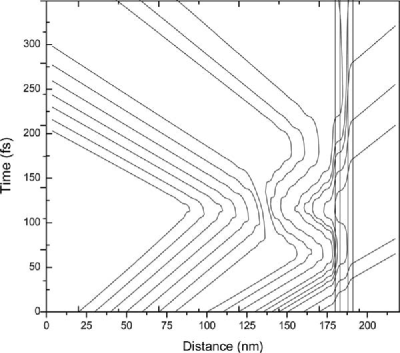
Figure 15: Representative Bohmian trajectories associated with double-packet scattering in a double-barrier potential. The position of the barriers is indicated by vertical lines. Reprinted with permission from om.oriolstime . Copyright 1996 American Physical Society.

To finish this practical computation of Bohmian trajectories from the direct solution of the time-dependent wave function, we can discuss some features of Bohmian trajectories related to the fact that they do not cross in the configuration space. We consider a quite “exotic” initial wave packet. We use a sum of two Gaussian wave packets defined by Eq. (LABEL:om.finite-difference_innitial) with different central positions and central (momenta) wave vectors om.oriolstime . The wave packet is certainly quite exotic because it describes just one particle. In Figs. 15 and 16 we see that Bohmian trajectories can be reflected for two different reasons: first, because of their interaction with the classical potential (the particles collide with the barrier) and, second, because of the collision with other trajectories traveling in the opposite direction (Bohmian trajectories do not cross). The second process is responsible for the reflection of those particles of the first packet, which never reach the barrier, and for the reflection of the entire second packet. These collisions between Bohmian particles are related to the quantum potential in regions where the classical potential is zero, but for them to occur, there should be particles coming from right to left. In this regard, if the initial wave packet is prepared as a superposition of eigenstates incident from left to right (as is always assumed in scattering thought experiments), and the classical potential is zero on the left-hand side (l.h.s.) of the barrier, then finding particles coming from the r.h.s. in this region will be at least very uncommon.

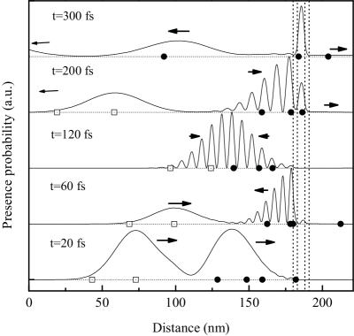
Figure 16: Picture motion of the same double-packet wave function considered in Fig. 15, calculated by numerical integration of the time-dependent Schrödinger equation. Five representative “snapshots” obtained at different times are shown with the vertical scale arbitrarily changed in each case for clarity. Although the norm of the wave function is always unity, it does not seem so because of the changes in the scale. The marks are visual aids that indicate the position of some related Bohmian trajectories shown in Fig. 15. The double-barrier position is indicated by the vertical dashed lines, and the arrows indicate the sense of motion of the two packets. Reprinted with permission from om.oriolstime . Copyright 1996 American Physical Society.

X.1.2 Time-independent Schrödinger equation for a 1D space (TISE_1D) with an implicit (matrix inversion) method

Next, we consider another very simple computational algorithm similar to the one discussed in the previous section (1D, analytic and explicit) but for time-independent systems. First, let us discuss under which circumstances we can expect that a time-independent Schrödinger equation can provide a reasonable physical description. Let us assume that the wave function $\psi(x,t)$ can be written as a product of a spatial function $\varphi(x)$ and a temporal function $\zeta(t)$, that is, $\psi(x,t)=\varphi(x)\zeta(t)$. Then, the Schrödinger equation, Eq. (163), with a time-independent potential $V(x)$ can be written as:

$$\frac{i\hbar\frac{\partial\zeta(t)}{\partial t}}{\zeta(t)}=\frac{-\frac{\hbar^{2}}{2m}\frac{{\partial}^{2}\varphi(x)}{\partial x^{2}}+V(x)\varphi(x)}{\varphi(x)}$$ (169)

Since the l.h.s. of Eq. (169) only depends on $t$ and the r.h.s. of Eq. (169) only depends on $x$, both sides are equal to a constant that we refer as $E$. Therefore, we obtain two separate equations:

$$i\hbar\frac{\partial\zeta(t)}{\partial t}=E\zeta(t)$$ (170)

$$-\frac{\hbar^{2}}{2m}\frac{{\partial}^{2}\varphi(x)}{\partial x^{2}}+V(x)\varphi(x)=E\varphi(x)$$ (171)

The first of these equations has a trivial analytical solution $\zeta(t)=e^{i\frac{Et}{\hbar}}$. However, the time-independent Schrödinger equation needs a numerical method to be solved for arbitrary shapes of the potential $V(x)$.

The second-order derivative can be approximated as:

$$\left.\frac{{{\partial}^{2}}\varphi\left(x\right)}{\partial{{x}^{2}}}\right|_{x=x_{k}}\approx\frac{\varphi(x_{k+1})-2\varphi(x_{k})+\varphi(x_{k-1})}{{\Delta x}^{2}}$$ (172)

Then, Eq. (171) can be written in a matrix representation as:

$$\left(-\frac{\hbar^{2}}{2m}\hat{\nabla}^{2}+\left(V(x_{k})-E\right)\hat{I}\right)\vec{\varphi}=0$$ (173)

where $\vec{\varphi}=(\varphi(x_{2}),\ldots,\varphi(x_{N-1}))^{T}$ is a $N-2$ vector, $\hat{{I}}$ is the $(N-2)\times(N-2)$ identity matrix and $\hat{\nabla}^{2}$ is the $(N-2)\times(N-2)$ matrix constructed from Eq. (172) as:

$$\hat{\nabla}^{2}=\frac{1}{{\Delta x}^{2}}\left(\begin{array}[c]{ccccc}-2&1&0&0&\ddots\\ 1&-2&1&0&\ddots\\ \ddots&\ddots&\ddots&\ddots&\ddots\\ \ddots&0&1&-2&1\\ \ddots&0&0&1&-2\end{array}\right)$$ (174)

The solution of $\vec{\varphi}$ can be found by inverting the matrix equation, Eq. (173). The (nonzero) solution of Eq. (173) requires that the determinant of the matrix be equal to zero. The determinant requirement is called the characteristic equation (less often, the secular equation). In our case, the determinant can only be zero for some particular values of the energy $E$ (i.e., quantized energies). Thus, this algorithm finds the eigenvalues $E$ and eigenvectors $\vec{\varphi}$, typical of a boundary value problem.

In the previous vector definition, $\vec{\varphi}$, only $N-2$ unknowns are considered. We have assumed that $\varphi(x_{1})=0$ and $\varphi(x_{N})=0$. This implies that $\vec{\varphi}$ is a real vector. Then, if we select an eigenstate, we realize that the current density is zero, $J(x,t)=0$, because $\varphi(x_{k})=\varphi(x_{k})^{*}$. All Bohmian velocities are zero, $\partial S/\partial x=0$, meaning that Bohmian trajectories do not “move.” This result is obviously consistent with the fact that the amplitude $R(x,t)$ of the global wave function $\psi(x,t)=\varphi(x)e^{-iEt/\hbar}$ is time independent. One is tempted to affirm that there is no kinetic energy for these Bohmian trajectories. However, as we see in Eq. (136), the evaluation of the mean value of the kinetic energy takes into account not only the Bohmian velocity but also the quantum potential. We can explain this point, differently, from the quantum Hamilton–Jacobi equation, Eq. (39). In our particular time-independent case, we have an energy conservation law:

$$V(x)-\frac{\hbar^{2}}{2m}\frac{{\partial}^{2}R(x)/\partial x^{2}}{R(x)}=E$$

where we have used $\partial S/\partial t=-E$ in Eq. (39). Then, we can obtain the following (time-independent Schrödinger-like) equation for the real wave function $R(x)$:

$$-\frac{\hbar^{2}}{2m}\frac{{\partial}^{2}R(x)}{\partial x^{2}}+V(x)R(x)=E\;R(x)$$ (175)

Comparing this expression with the previous Eq. (171), we realize that in this particular problem (for which all Bohmian trajectories have zero velocity), the quantum potential takes the role of a “kinetic” energy.

X.1.3 Time-independent Schrödinger equation for a 1D space (TISE_1D) with an explicit method

We can also look for a very simple explicit algorithm to find the solution $\vec{\varphi}$ of the time-independent Schrödinger equation. Equation (171) is a homogeneous second-order differential equation that can be written as:

$$\frac{{d}^{2}}{d{x}^{2}}\varphi(x)=f(x)\psi(x)$$ (176)

where $f(x)$ is the constant of proportionality between the solution and the second derivative at each point:

$$f(x)=\frac{2m}{{\hbar}^{2}}(V(x)-{E})$$ (177)

From the Taylor expansion for $\varphi(x_{k+1})$ around $x_{k}$, we get:

$$\varphi(x_{k+1})= \varphi(x_{k})+\Delta x\left.\frac{d\varphi(x)}{dx}\right|_{x=x_{k}}+\frac{\Delta x^{2}}{2!}\left.\frac{d^{2}\varphi(x)}{dx^{2}}\right|_{x=x_{k}}+\,\left.\frac{\Delta x^{3}}{3!}\frac{d^{3}\varphi(x)}{dx^{3}}\right|_{x=x_{k}}$$ (178)

$$+\frac{\Delta x^{4}}{4!}\left.\frac{d^{4}\varphi(x)}{dx^{4}}\right|_{x=x_{k}}+\,\frac{\Delta x^{5}}{5!}\left.\frac{d^{5}\varphi(x)}{dx^{5}}\right|_{x=x_{k}}+{O}(h^{6})$$

Identically, for $\varphi(x_{k-1})$ around $x_{k}$, we get:

$$\varphi(x_{k-1})= \varphi(x_{k})-\Delta x\left.\frac{d\varphi(x)}{dx}\right|_{x=x_{k}}+\frac{\Delta x^{2}}{2!}\left.\frac{d^{2}\varphi(x)}{dx^{2}}\right|_{x=x_{k}}-\,\frac{\Delta x^{3}}{3!}\left.\frac{d^{3}\varphi(x)}{dx^{3}}\right|_{x=x_{k}}$$ (179)

$$+\frac{\Delta x^{4}}{4!}\left.\frac{d^{4}\varphi(x)}{dx^{4}}\right|_{x=x_{k}}-\,\frac{\Delta x^{5}}{5!}\left.\frac{d^{5}\varphi(x)}{dx^{5}}\right|_{x=x_{k}}+{O}(\Delta x^{6})$$

The sum of these two equations gives:

$$\varphi(x_{k+1})+\varphi(x_{k-1})= 2\varphi(x_{k})+{\Delta x^{2}}\left.\frac{d^{2}\varphi(x)}{dx^{2}}\right|_{x=x_{k}}+\,\frac{\Delta x^{4}}{12}\left.\frac{d^{4}\varphi(x)}{dx^{4}}\right|_{x=x_{k}}+{O}(\Delta x^{6})$$

We use Eq. (176) to define, directly, the second-order derivative. We compute the fourth-order derivative from a second-order derivative written as a difference quotient. Finally, we find a recursive expression for the wave function $\varphi(x_{k-1})$:

$$\varphi(x_{k-1})=\frac{\left[2+\frac{10}{12}{\Delta x}^{2}f(x_{k})\right]\varphi(x_{k})-\left[1-\frac{{\Delta x}^{2}}{12}f(x_{k+1})\right]\varphi(x_{k+1})}{1-\frac{{\Delta x}^{2}}{12}f(x_{k-1})}$$ (181)

We have explicitly written $\varphi(x_{k-1})$ in Eq. (181) because later, in a numerical example, we will be interested in specifying the boundary conditions of $\varphi(x)$ at $x\rightarrow\pm\infty$. The Numerov method om.numrov1 ; om.numrov2 provides a numerical algorithm to solve ordinary differential equations of the second order in which the first-order term does not appear. It is a fourth-order linear multistep method. The above expression, Eq. (181), allows a simple solution of $\varphi(x_{k-1})$ once we know $\varphi(x_{k})$, $\varphi(x_{k+1})$, $f(x_{k})$, $f(x_{k+1})$, and $f(x_{k-1})$. Finally, repeating the process, we can determine the entire solution.

We will apply this last explicit computational algorithm for tunneling scenarios. For the numerical simulations, we will use $\Delta x=1$ Å. Again, the amplitude of the global wave function $\psi(x,t)=\varphi(x)e^{-iEt/\hbar}$ is time independent. Thus, the current density $J(x,t)$, from Eq. (34), is also time independent. Therefore, from the continuity equation, Eq. (28), we deduce that $J(x,t)$ is also uniform (position-independent). Then, the velocity $v(x)=$ constant$/R^{2}(x)$ does not depend on time but depends on position. We have $S(x,t)\neq 0$. The velocity can be computed from:

$$\frac{\partial S(x,t)}{\partial x}=\sqrt{2m(E-V(x)-Q(x))}$$ (182)

See problem 11 for a detailed calculation. This quantum expression, Eq. (182), is different from the similar expression extracted from the classical Hamilton–Jacobi equation ${\partial S(x,t)}/{\partial x}=\sqrt{2m(E-V(x))}$. When $E<V(x)$, we will not be able to find a (real) velocity in a classical system (classical particles are unable to pass through spatial regions where the potential barrier is higher than its energy). Interestingly, when $E<V(x)$ in Eq. (182), we will still find (real) velocities because of the term $Q(x)$ in Eq. (182) (Bohmian particles are able to pass through spatial regions where the potential barrier is higher than its energy). This is the well-known tunneling effect.

As a numerical example, let us concentrate on (time- independent) scattering states traveling from left to right in a double-barrier structure. For a simulation box $0<x<40\;\rm nm$, these states can be written as:

$$\varphi(x)=\frac{1}{\sqrt{2\pi}}\left(e^{ikx}+r(k)e^{-ikx}\right)\;\;;\;\;\;x<0\;\rm nm$$ (183)

$$\varphi(x)=\frac{1}{\sqrt{2\pi}}\left(t(k)e^{ikx}\right)\;\;;\;\;\;x>40\;\rm nm$$ (184)

where $r(k)$ and $t(k)$ are (unknown) complex coefficients accounting for reflection and transmission, respectively. However, up to an irrelevant (complex) constant that can be fixed by “normalization,” we know the results $\varphi(x)$ at $x\rightarrow\pm\infty$. In the central region, we can use the Numerov numerical method using the fact that the wave function and its derivative have to be continuous in the matching points between the regions where we have analytical or numerical knowledge of the wave functions.

In Fig. 17, we have represented one Bohmian trajectory for a state incident from left to right upon a double-barrier potential profile. Its energy $E=0.05$ eV corresponds to the first resonant level of the double barrierom.oriols_sst . In this particular case, where the transmission coefficient is very close to unity, the results obtained within the Bohmian approach are quite compatible with our intuitive understanding of the tunneling phenomenon: the particle is transmitted, and its velocity decreases in the well. We do also plot the total potential-that is, the sum $V(x)+Q(x)$-which is lower than the electron energy $E=0.05$ eV.

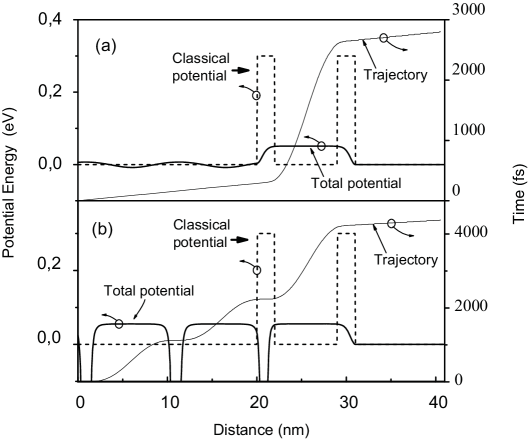
Figure 17: Bohmian trajectories associated with stationary scattering states impinging on a typical GaAs/AlGaAs RTD with 2 nm barriers of 0.3 eV separated by a 7 nm well. The classical potential and the total potential (the sum of classical and quantum terms) are also depicted in dashed and solid lines, respectively. (a) Resonant eigenstate, $E_{k}=0.05$ eV; (b) nonresonant eigenstate, $E_{k}=0.0$6 eV. Reprinted with permission from om.oriols_sst . Copyright 1996 Elsevier. Abbreviation: RTD, resonant tunneling diode.

However, the situation is far from intuitive for nonresonant states. In Fig. 17b, we have represented one of these nonresonant trajectories for the same potential profile. Now, although the transmission coefficient is much smaller than unity for the nonresonant states, they present the same features as the resonant ones: all Bohmian trajectories are transmitted through the barrier. This fact can be easily understood from a mathematical point of view. As we mentioned, the current and particle densities are time independent and positive everywhere. So, the Bohmian velocity is always positive. In this regard, although Bohmian trajectories associated with scattering states perfectly reproduce the presence probability and the current density, they do not reproduce our particle-intuitive understanding of the tunneling phenomenon, since in principle, we would expect reflected as well as transmitted trajectories. The origin of this lack of intuitive behavior of Bohmian trajectories is only due to the initial wave function that we select. The velocity of Bohmian particles is neither related to the incident electron nor related to the reflected one but to the average of both because the wave function itself is defined as a weighted sum of waves with positive and negative momentum. In particular, if the barrier is infinitely high, then the reflection coefficient is equal to one and Bohmian’s velocity is zero (one would expect positive and negative electron velocities). Transport is better formulated as a time-dependent process. A time dependent picture of transport involves a wave packet with a well defined initial velocity and, after the interaction, a well-defined reflected (or transmitted) velocity, but not a unique velocity with an average of incident and reflected velocities.

All the 1D numerical algorithms previously discussed can be easily generalized to 2D and 3D systems (see, for example, the solution of the Schrödinger equation for computing Bohmian trajectories in atomic scenarios in Refs. om.mompart1 ; om.mompart2 ). However, the computational burden of such techniques with finite-difference meshes is enormous, and the solution using adaptative meshes seems interesting. For example, the triangular mesh generated using an algorithm inspired by Ref. om.Persson , with Delaunay refinement algorithms, yields a final mesh that is surprisingly well shaped, resulting in an excellent support to solve partial differential equations, as it was remarked in Ref. om.Pinto .

X.2 Synthetic computation of Bohmian trajectories

Up to here, we have only discussed analytical algorithms to find Bohmian trajectories. However, it is possible to compute Bohmian trajectories without knowing the wave function. The key point is using the polar form $\psi(\vec{r},t)=R(\vec{r},t)\exp(iS(\vec{r},t)/\hbar)$ to obtain the quantum Hamilton–Jacobi equations. As we anticipated, these new equations are nonlinear in $R(\vec{r},t)$ and $S(\vec{r},t)$. We will now discuss the advantages and disadvantages of numerically solving the quantum Hamilton–Jacobi equation, Eq. (39). Hereafter, we will analyze two different algorithms to solve numerically Eq. (39). First, directly solving these equations (the Eulerian formalism) or some equivalent variable change . Second rewriting the Hamilton–Jacobi equations within the Langrangian formalism and solving them.

The first point that we want to clarify is that, although the function $S(\vec{r},t)$ is in principle multivalued, the numerical solution of $S(\vec{r},t)$ has a unique value at each point $\vec{r}$ and $t$. The reason is because of an important theorem on the existence and uniqueness of solutions to first-order equations with given initial-value problems. See page 70 in om.perko .

X.2.1 Time-dependent quantum Hamilton–Jacobi equations (TDQHJE_1D) with an implicit (Newton-like fixed Eulerian mesh) method

In the Eulerian formalism, we use a fixed grid. We are interested in providing a discussion valid for 1D, 2D, and 3D spatial scenarios. Therefore, we define a grid in real space through a set of discrete vectors $\vec{p}_{i}$ for $i=1,\ldots,N$-in particular, $\vec{p}_{i}=(x_{i},y_{i},z_{i})$ for a 3D space, $\vec{p}_{i}=(x_{i},y_{i})$ for a 2D space, and $\vec{p}_{i}=(x_{i})$ for 1D. In order to provide a compact notation, we define:

$$\vec{R}_{j}=\left(R_{j}(\vec{p}_{1}),\ldots,R_{j}(\vec{p}_{N})\right)^{T}$$ (185)

$$\vec{S}_{j}=\left(S_{j}(\vec{p}_{1}),\ldots,S_{j}(\vec{p}_{N})\right)^{T}$$ (186)

$$\vec{V}_{j}=\left(V_{j}(\vec{p}_{1}),\ldots,V_{j}(\vec{p}_{N})\right)^{T}$$ (187)

where $R_{j}(\vec{p}_{i})=R(\vec{r},t)$ at $t=t_{j}$ and $\vec{r}=\vec{p}_{i}$ (identically for $S_{j}(\vec{p}_{i})=S(\vec{r},t)$ and $V_{j}(\vec{p}_{i})=V(\vec{r},t)$). We have also used a mesh in time $t_{j}=j\Delta t$ for $j=1,\ldots,M$

In the definition of the temporal derivatives of the quantum Hamilton–Jacobi, we can use an implicit expression, Eq. (162), or an explicit one, Eq. (160). The explicit expression will lead to an algorithm similar to the one described in Sec. X.1.1 with the same advantages (simplicity) and disadvantages (i.e., conditional stable). In this section, we will explore the implicit route. Then, the discrete version of the quantum Hamilton–Jacobi equations, Eq. (39), reads:

$$\frac{\vec{R}_{j}^{2}-\vec{R}_{j-1}^{2}}{\Delta t}+\hat{\nabla}\left(\frac{\vec{R}_{j}^{2}\hat{\nabla}\vec{S}_{j}}{m}\right)=0$$

$$\frac{\vec{S}_{j}-\vec{S}_{j-1}}{\Delta t}+\frac{(\hat{\nabla}\vec{S}_{j})^{2}}{2m}-\frac{\hbar^{2}}{2m}\frac{\hat{\nabla}^{2}\vec{R}_{j}}{\vec{R_{j}}}+\vec{V_{j}}=0$$

The operations such as power, multiplication, and division between the vectors $\vec{X}_{j}$ and $\vec{Y}_{j}$ are understood over each point in the spatial mesh, that is:

$$\vec{X}_{j}\vec{Y}_{j}=[X_{j}(\vec{p}_{1})Y_{j}(\vec{p}_{1}),\ldots,X_{j}(\vec{p}_{N})Y_{j}(\vec{p}_{N})]^{T}$$ (189)

Here the symbol $\hat{\nabla}$ is the matrix representation of the differential operator $\vec{\nabla}$ in the 1D, 2D, or 3D spatial mesh. The representation of $\hat{\nabla}$ depends in general on the choice of the spatial mesh and on how the spatial derivatives are approximated. For example, in a 1D system with a uniform mesh step size $\Delta x$, the discrete version of the spatial derivative in one dimension is:

$$\frac{\partial R(x,t)}{\partial x}=\frac{R_{j}(\vec{p}_{i+1})-R_{j}(\vec{p}_{i-1})}{2\Delta x},$$ (190)

with $\vec{p}_{i}=x_{0}+i\Delta x$. Then, the nabla operator in one dimension $\hat{\nabla}_{1D}$ is represented by the following matrix:

$$\hat{\nabla}_{1D}=\frac{1}{2\Delta x}\left(\begin{array}[c]{ccccc}2&-2&0&0&\ddots\\ 1&0&-1&0&\ddots\\ \ddots&\ddots&\ddots&\ddots&\ddots\\ \ddots&0&1&0&-1\\ \ddots&0&0&-2&2\end{array}\right)$$ (191)

Notice that we have changed the definition of the spatial derivative from Eq. (190) in $x_{1}$ and $x_{N}$. In two or three dimensions the matrices still have many zeros with the entries $1$ and $-1$ properly located.

Hereafter, as we mentioned, we only discuss the computational problems of the implicit solution of the Hamilton–Jacobi equations. Such an equation is nonlinear with respect to $\vec{R}_{j}$ and $\vec{S}_{j}$, and the matrix inversion explained in Sec. X.1.2 cannot be done. Then, in order to find the numerical solution of the discrete version of Eq. (X.2.1), we have to employ some Newton-like method. If we rewrite in compact form the Eq. (X.2.1) as:

$$F(\vec{R}_{j},\vec{S}_{j})=0$$ (192)

then we have to find the roots (zeros) of the nonlinear expression in Eq. (192). It is proved that the sequence:

$$\left(\begin{array}[c]{c}\vec{R}_{j}^{(h+1)}\\ \vec{S}_{j}^{(h+1)}\end{array}\right)=-J_{F}^{-1}(\vec{R}_{j}^{(h)},\vec{S}_{j}^{(h)})\left(\begin{array}[c]{c}\vec{R}_{j}^{(h)}\\ \vec{S}_{j}^{(h)}\end{array}\right)$$ (193)

where $J_{F}(\vec{R}_{j}^{(h)},\vec{S}_{j}^{(h)})$ is the Jacobian of $F(\vec{R}_{j}^{(h)},\vec{S}_{j}^{(h)})$, for suitable initial vectors $\vec{R}_{j}^{(0)}$ and $\vec{S}_{j}^{(0)}$, converges quadratically to the solution of Eq. (192) for $h\rightarrow\infty$. Thus the key of this approach is to solve the linear system in Eq. (193). However evaluating explicitly the Jacobian:

$$J_{F}(\vec{R}_{j},\vec{S}_{j})=\left(\!\begin{array}[c]{@{}c@{\ }c@{}}\frac{2}{\Delta t}\hat{diag}(\vec{R}_{j})+\hat{\nabla}\left(\hat{diag}\left(\frac{2\vec{R}_{j}\hat{\nabla}\vec{S}_{j}}{m}\right)\right)&\hat{\nabla}\hat{diag}\left(\frac{\vec{R}_{j}^{2}}{m}\right)\hat{\nabla}\\ -\frac{\hbar^{2}}{2m}\hat{diag}\left(\!\frac{1}{\vec{R}_{j}}\!\right)\hat{\nabla}^{2}-\hat{diag}\left(\!\frac{\hat{\nabla}^{2}\vec{R}_{j}}{\vec{R}_{j}^{2}}\!\right)&\frac{1}{\Delta t}\hat{diag}(\vec{S}_{j})+\hat{diag}\left(\frac{\hat{\nabla}\vec{S}_{j}}{m}\right)\hat{\nabla}\end{array}\!\right)$$ (196)

where:

$$\hat{diag}(\vec{X}_{j})=\left(\begin{array}[c]{ccccc}{X}_{j}(\vec{p}_{1})&0&0&0&\ddots\\ 0&{X}_{j}(\vec{p}_{2})&0&0&\ddots\\ \ddots&\ddots&\ddots&\ddots&\ddots\\ \ddots&0&0&{X}_{j}(\vec{p}_{N-1})&0\\ \ddots&0&0&0&{X}_{j}(\vec{p}_{N})\end{array}\right)$$ (198)

we can readily recognize that for small components of $\vec{R}_{j}$, the Jacobian is ill conditioned and the system of Eq. (193) is impossible to be solved numerically. Unfortunately this is the case of localized particles where $\vec{R}_{j}$ become exponentially small far from the central position of the particles. This problem does not appear with the explicit algorithm for solving the quantum Hamilton–Jacobi equations. The problem can also be avoided by choosing the variable change $\psi(\vec{r},t)=\exp(C(\vec{r},t)+iS(\vec{r},t)/\hbar)$ allowing to the equations:

$$\frac{\partial}{\partial t}C(\vec{r},t)=-\frac{1}{2m}\left(\nabla^{2}S(\vec{r},t)+2\vec{\nabla}S(\vec{r},t)\cdot\vec{\nabla}C(\vec{r},t)\right)$$

$$\frac{\partial}{\partial t}S(\vec{r},t)=-\frac{(\vec{\nabla}S(\vec{r},t))^{2}}{2m}+\frac{\hbar^{2}}{2m}\left(\nabla^{2}C(\vec{r},t)+(\vec{\nabla}C(\vec{r},t))^{2}\right)-V(\vec{r},t)$$

However, the advantage of this method carries out also its disadvantage. The limitation of this approach is that the functions $S(\vec{r},t)$ and $C(\vec{r},t)$ strongly vary in the entire simulation space. Thus when we account for a realistic situation for which a large simulation space is used, the computational problem can become very hard because the number of space mesh points $\vec{p}_{k}$ will be quite large to obtain an accurate solution.

X.2.2 Time-dependent quantum Hamilton–Jacobi equations (TDQHJE_1D) with an explicit (Lagrangian mesh) method

A different approach to solve the quantum Hamilton–Jacobi equation is based on the Lagrangian picture. The basic idea is to use as a grid the Bohmian trajectories themselves. In this picture, the point $\vec{p}_{k}$ is no longer a fixed spatial point but a time-dependent point $\vec{p}_{k}=\vec{p}_{k}(t)$ with $k=1,\ldots,N$ moving with instantaneous velocity $\vec{v}_{k}(t)$. For a detailed analysis see Refs. om.Wyatt1 ; om.Wyatt2 ; om.Wyatt3 ; om.Frederick .

To pass from the Eulerian to the Lagrangian hydrodynamic picture, we must be careful with the time derivative of the functions $R(\vec{p}_{k}(t),t)$, $S(\vec{p}_{k}(t),t)$ and $V(\vec{p}_{k}(t),t)$. We have to use the chain rule:

$$\frac{d}{dt}=\frac{\partial}{\partial t}+\vec{v}(\vec{r},t)\cdot\vec{\nabla}$$ (200)

which includes the convective term $\vec{v}(\vec{r},t)\cdot\vec{\nabla}$ with the velocity defined:

$$\vec{v}(\vec{r},t)=\frac{1}{m}\vec{\nabla}S(\vec{r},t)$$ (201)

The new equations derived from the quantum Hamilton–Jacobi equations (or equivalently from Eq. (X.2.1)) can be written as:

$$\frac{d}{dt}\vec{p}_{k}(t)=\vec{v}(\vec{p}_{k}(t),t)$$ (202)

$$\frac{d}{dt}S(\vec{p}_{k}(t),t)=\frac{(\vec{\nabla}S(\vec{p}_{k}(t),t))^{2}}{2m}+\frac{\hbar^{2}}{2m}\frac{\nabla^{2}R(\vec{p}_{k}(t),t)}{R(\vec{p}_{k}(t),t)}-V(\vec{p}_{k}(t),t)$$ (203)

$$\vec{v}(\vec{p}_{k}(t),t)=\frac{1}{m}\vec{\nabla}S(\vec{p}_{k}(t),t)$$ (204)

$$\frac{d}{dt}R(\vec{p}_{k}(t),t)=-\frac{1}{2}R(\vec{p}_{k}(t),t)\vec{\nabla}\cdot\vec{v}(\vec{p}_{k}(t))$$ (205)

The differential system in Eqs. (202–205) is written for the trajectory $\vec{p}_{k}(t)$ with a particular initial position $\vec{p}_{k}(0)$. However to (numerically) reproduce the wave function $\psi(\vec{r},t)=R(\vec{r},t)\exp(iS(\vec{r},t)/\hbar)$ defined in the entire space, we have to deal with $k=1,\ldots,N$ trajectories with $N\rightarrow\infty$. The distribution of their initial positions $\vec{p}_{k}(0)$ has to be obtained according to the squared modulus of the initial wave function $|\psi(\vec{p}_{k}(0),0)|^{2}$, that is, the quantum equilibrium hypothesis described in Sec. V.6. See also Ref. om.Holand1993 . Thus, by construction we are using a mesh that is continuously adapting to the wave function time evolution because the Bohmian trajectories themselves follow the wave function.

In this picture the strategy to solve Eqs. (202–205) can be very complicated om.Wyatt1 ; om.Wyatt2 ; om.Wyatt3 ; om.Frederick . However, some simple consideration can be done in order to understand the limits of this approach. The method widely used om.Wyatt1 ; om.Wyatt2 ; om.Wyatt3 ; om.Frederick to integrate Eqs. (202–205) is to solve them in cascade with the following approximations: at time $t_{j}$ the new trajectories positions are computed through:

$$\vec{p}_{j,k}=\vec{p}_{j-1,k}+\Delta t\vec{v}_{j-1,k}$$ (206)

with $\vec{p}_{j,k}=\vec{p}_{k}(t_{j})$. In the updated grid defined by $\vec{p}_{j,k}$, the variables ${S}_{j}(\vec{p}_{j,k})$, $\vec{v}_{j}(\vec{p}_{j,k})$, and $\vec{R}_{j}(\vec{p}_{j,k})$ are evaluated by:

$${S}_{j}(\vec{p}_{j,k}) = {S}_{j-1}(\vec{p}_{j,k})+\Delta t\Bigg{[}\frac{(\hat{\nabla}_{j-1}{S}_{j-1}(\vec{p}_{j,k}))^{2}}{2m}+\,\frac{\hbar^{2}}{2m}\frac{\hat{\nabla}_{j-1}^{2}{R}_{j-1}(\vec{p}_{j,k})}{{R}_{j-1}(\vec{p}_{j,k})}-\vec{V}_{j-1}(\vec{p}_{j,k})\Bigg{]}$$

$${R}_{j}(\vec{p}_{j,k}) = {R}_{j-1}(\vec{p}_{j,k})-\Delta t\left[\frac{1}{2m}{R}_{j-1}(\vec{p}_{j,k})\hat{\nabla}_{j-1}^{2}\vec{S}_{j-1}(\vec{p}_{j,k})\right]$$

$${v}_{j}(\vec{p}_{j,k}) = \frac{1}{m}\hat{\nabla}_{j}\vec{S}_{j}(\vec{p}_{j,k})$$

where $\hat{\nabla}_{j}$ is the gradient operator evaluated in $\vec{p}_{j,k}$ through efficient interpolation methods om.Wyatt1 ; om.Wyatt2 ; om.Wyatt3 ; om.Frederick . It can be realized that we have used an (unstable) explicit (forward Euler) time integration method om.Striwerda to avoid the computational burden associated with implicit methods with nonlinear equations discussed before. This limitation (small temporal step to ensure stable solutions) is made worse since the time step must be further reduced when some trajectory approaches points for which the potential $V$ and/or the quantum potential $Q$ strongly varies provoking large variations of some $\vec{v}_{j}$.

The variables $S$ and $\vec{v}$ vary in the entire simulation space; thus when we account for a realistic situation such that a large simulation space is used, the computational problem can become very hard due to the fact that the number of space mesh points $\vec{p}_{k}$ can diverge to obtain an accurate solution. On the contrary, this method has some fundamental advantage over methods using fix grid points. In the latter, the extension of 1D algorithms to 2D and 3D algorithms means increasing exponentially the number of grip points. However, in the former methods (i.e., when the grid points are Bohmian trajectories), the number of points can be chosen by the user. Thus, for exemple, one can simulate a 1D system with 1,000 Bohmian trajectories (grid points) and a 2D system with  3,000 Bohmian trajectories (grid points).

X.3 More elaborated algorithms

We have presented very simple and easily implementable codes for computing Bohmian trajectories in simple scenarios. These algorithms can be used for newcomers to be introduced to the computation of quantum dynamics with Bohmian mechanics. Certainly, there are many more elaborated and “professional” computational algorithms in the literature. An excellent source of information on this issue can be found in the book written by R. E. Wyatt entitled Quantum Dynamics with Trajectories: Introduction to Quantum Hydrodynamics om.wyatt2005 .

To end this section, we want to briefly mention some original and powerful techniques, inspired by Bohmian mechanics, available in the literature, whose explicit description is far from the scope of this introductory appendix. Recently, B. Poirier showed how Bohmian trajectories can be computed for 1D eigenstates without the wave function om.poirier . The work of N. Makri shows the possibility of using imaginary time algorithms to estimate eigenstates and eigenvalues om.imaginarytime . With a similar goal, I. P. Christov uses quantum trajectories to develop time-dependent quantum Monte Carlo algorithms om.ivan ; om.ivan2 . We also mention the work of E. L. Bittner om.extra16 developed in chapter 5 in this book. The work presented in Sec. VI.6 can also be interpreted as an approximating technique for computing many-particle systems om.oriolsprl . This last work has been used by the group of Oriols to develop a powerful quantum electron transport simulator. ( http://europe.uab.es/bitlles). See Refs. om.oriolsexample1 ; om.oriolsexample2 or chapter 6 for practical results on electron correlation in nanoelectronics. Another line of work is also devoted to the approximation of the quantum potential. See, for example, the work of S. Garashchuk and V. A. Rassolov om.gara . The correlation between classical and quantum systems has also been studied extensively. See, for example, Ref. om.extra13 ; om.5marian ; om.6colomes . We do also highlight the work by D. J. Tannor and coworkers on the use of imaginary quantum trajectories (complex action) for quantum dynamics om.imaginaryaction ; om.imaginaryactionprl . We also want to notice the important amount of work done by many people in the field of ab-initio molecular dynamics, specially for tackling the coupled electron-nuclear motion in nonadiabatic electronic transitions om.extra18 ; om.extra19 ; om.extra20 ; om.extra21 ; om.extra22 ; om.extra23 ; om.extra24 . Finally, we mention the more recent work by L. B. Madsen and co-workers in the field of bosonic systems om.extra25 .

All the works mentioned have been elaborated during the past 18 years after the pioneering work of Wyatt om.Wyatt1 ; om.extra17 . Much work is still needed to evaluate the real capability of synthetic applications of Bohmian mechanics as a computational tool.

References

- (1) M. Planck, On the Law of Distribution of Energy in the Normal Spectrum, Annalen der Physik 4, 553 (1901).
- (2) A. Einstein, ber einen die Erzeugung und Verwandlung des Lichtes betreffenden heuristischen Gesichtspunkt, Annalen der Physik 17, 132 (1905).
- (3) N. Bohr, On the Constitution of Atoms and Molecules, Part I, Philosophical Magazine 26, 1 (1913).
- (4) N. Bohr, On the Constitution of Atoms and Molecules, Part II Systems Containing Only a Single Nucleus, Philosophical Magazine 26, 476 (1913).
- (5) N. Bohr, On the Constitution of Atoms and Molecules, Part III Systems Containing Several Nuclei, Philosophical Magazine 26, 857 (1913).
- (6) L. de Broglie, Recherches sur la théorie des quantas, Ann. de Physique 3, 22 (1925).
- (7) L. de Broglie La mécanique ondulatorie et la structure atomique de la matière et du rayonnement, Journal de Physique et du Radium 8, 225 (1927).
- (8) D. Bohm, A suggested interpretation of the quantum theory in terms of “hidden” variables I, Phys. Rev. 85, 166 (1952).
- (9) D. Bohm, A suggested interpretation of the quantum theory in terms of “hidden” variables II, Phys. Rev. 85, 180, (1952).
- (10) M. Born, Zur Quantenmechanik der Sto vorgänge, Zeitschrift für Physik 37, 863 (1926).
- (11) W. Heisenberg, Über quantentheoretishe Umdeutung kinematisher und mechanischer Beziehungen, Zeitschrift für Physik 33, 879 (1925); English translation in Ref. om.waerden .
- (12) J. von Neumann, Mathematische Grundlagen der Quantenmechanik (Springer Verlag, Berlin 1932); English translation by: R. T. Beyer, Mathematical Foundations of Quantum Mechanics (Princeton University Press, Princeton 1955).
- (13) J. S. Bell, 1987, Speakable and Unspeakable in Quantum Mechanics (Cambridge University Press, Cambridge 1987).
- (14) A. Einstein, Physics and reality Journal of the Franklin Institute 221(3), 349 (1936).
- (15) E. Wigner, The Unreasonable Effectiveness of Mathematics in the Natural Sciences, Communications on Pure and Applied Mathematics 13, 1 (1960).
- (16) N. Herbert, Quantum reality (Anchor Books, New York 1984).
- (17) “If, in some cataclysm, all of scientific knowledge were to be destroyed, and only one sentence passed on to the next generations of creatures, what statement would contain the most information in the fewest words? I believe it is the atomic hypothesis (or the atomic fact, or whatever you wish to call it) that all things are made of atoms—little particles that move around in perpetual motion, attracting each other when they are a little distance apart, but repelling upon being squeezed into one another. In that one sentence, you will see, there is an enormous amount of information about the world, if just a little imagination and thinking are applied.” R. P. Feynman, R. B. Leighton and M. Sands, Feynman Lectures on Physics (Addison-Wesley, Caltech USA 1965).
- (18) G. Binnig, H. Rohrer, C. Gerber, and E.Weibel, Surface Studies by Scanning Tunneling Microscopy, Physical Review Letters 49, 57 (1982).
- (19) Private exchange of letters between S. Goldstein and S. Weinberg; http://www.mathematik.uni-muenchen.de/~bohmmech/BohmHome/weingold.htm
- (20) R. E. Wyatt Quantum Dynamics with Trajectories: Introduction to Quantum Hydrodynamics (Springer, 2005).
- (21) A. Valentini, Pilot-Wave Theory: An Alternative Approach to Modern Physics (Cambridge University Press, Cambridge 2006).
- (22) G. Bacciagaluppi and A. Valentini, Quantum Theory at the Cross-roads: Reconsidering the 1927 Solvay Conference (Cambridge University Press, Cambridge 2009).
- (23) D. Peat Infinite Potential: the life and times of David Bohm (Helix Books, Addison-Wesley Publishing Company, Inc. 1997)
- (24) P. R. Holland, The Quantum Theory of Motion: An account of the de Broglie-Bohm Causal Interpretation of Quantum mechanics (Cambridge University Press, Cambridge 1993).
- (25) S. W. Saunders et al. Everett and his Critics (Oxford University Press, 2009) and arXiv: quant-ph/0811081.
- (26) J. T. Cushing, A. Fine and S. Goldstein, Bohmian Mechanics and Quantum Theory: An Appraisal (Kluwer Academic Publishers, 1996)
- (27) Private communication with Basile Hiley and David Peat
- (28) D. Bohm and B. J. Hiley. The Uundivided Universe: An Ontological Intepretation of Quantum Theory (Routledge & Kegan Paul, London, 1993).
- (29) E. Madelung, Quantentheorie in hydrodynamischer Form, Z. Phys. 40, 322 (1926).
- (30) http://www.isiknowledge.com/
- (31) L. de Broglie, Recherches sur la théorie des quantas, PhD thesis, University of Paris (1924); see also om.dB_AnnPhys .
- (32) G. N. Lewis, The Conservation of Photons, Nature 118(2), 874 (1926); See also http://www.nobeliefs.com/photon.htm
- (33) B. L. van der Waerden, Sources of Quantum Mechanics (Dover Publications, 1968).
- (34) W. Heisenberg, Über den anschaulichen Inhalt der quantentheoretischen Kinematik und Mechanik, Zeitschrift für Physik 43(3–4), 172 (1927).
- (35) M. Born and P. Jordan, Zur Quantenmechanik, Zeitschrift für Physik 34, 858 (1925); English translation in Ref. om.waerden .
- (36) M. Born, W. Heisenberg, and P. Jordan, Zur Quantenmechanik II, Zeitschrift für Physik 35, 557 (1925); English translation in Ref. om.waerden .
- (37) E. Schrödinger, An Undulatory Theory of the Mechanics of Atoms and Molecules, Physical Review 28, 1049 (1926).
- (38) B. L. van der Waerden, From Matrix Mechanics and Wave Mechanics to Unified Quantum Mechanics, Notices of the AMS 44, 323 (1997).
- (39) D. Bohm, Quantum Theory (Dover Publications, New York, 1951).
- (40) N. D. Mermin, What’s Wrong with This Pillow?, Physics Today 42(4), 9 (1989).
- (41) N. D. Mermin, Could Feynman Have Said This?, Physics Today 57(5), 10 (2004).
- (42) L. de Broglie, Tentative d’interpretation causale et non-lineairie de la mecanique ondulatorie (Gauthier-Villars, Paris, 1956).
- (43) http://www.alberteinstein.info/db/ViewDetails.do?DocumentID = 34338; explained also in om.Hollaneinstein .
- (44) P. R, Holland, What’s Wrong with Einstein’s 1927 Hidden-Variable Interpretation of Quantum Mechanics?, Foundations of Physics, 35(2) 177 (2005).
- (45) D. Bohm, on an interview in 1987; see http://www.fdavidpeat.com/interviews/bohm.htm
- (46) A. Einstein, B. Podolsky, and N. Rosen, Can Quantum Mechanical Description of the Physical Reality Be Considered Complete? Physics Review 47, 777 (1935).
- (47) C. Cohen-Tanoudji, B. Diu, and F. Laloë, Quantum Mechanics (Wiley, New York, 1977).
- (48) H. Nikolic, Would Bohr Be Born if Bohm Were Born before Born?, Am. J. Phys. 76, 143 (2008).
- (49) M. Gell-Mann, The Nature of the Physical Universe: The 1976 Nobel Conference (Wiley, New York, 1979); M. Gell-Mann presented his Nobel lecture but did not submit the manuscript for inclusion in the official volume. He explains: I did have a written version of the lecture that I gave in Sweden, but I was not satisfied with it and did not submit it …I tried to write a better one, including an adequate discussion of quarks, and agonized over it for months, but in the end, I did not finish it in time for it to be included in the volume..
- (50) J. S. Bell, On the Einstein Podolsky Rosen Paradox Physics 1, 195 (1964).
- (51) J. S. Bell, On the Impossible Pilot Wave, Foundations of Physics 12, 989 (1982). Reprinted in om.Bell1987 .
- (52) J. S. Bell, Against Measurement, Physics World 3, 33 (1990).
- (53) H. P. Stapp, Are Superluminal Connections Necessary?, Il Nuovo Cimento 40B, 191 (1977).
- (54) A. Aspect, P. Grangier, and G. Roger, Experimental Realization of Einstein-Podolsky-Rosen-Bohm Gedankenexperiment: A New Violation of Bell’s Inequalities, Physical Review Letters 49(2), 91 (1982).
- (55) D. Kleppner and R. Jackiw, One Hundred Years of Quantum Physics, Science 289(5481), 893 (2000).
- (56) T. Takabayasi, On the Formulation of Quantum Mechanics Associated with Classical Pictures, Progress of Theoretical Physics 8, 143 (1952).
- (57) It is written in Ref. om.Bohmian1996 by Professor J. T. Cushing, himself, that he submitted a research proposal to the US National Science Foundation for theoretical work to be done, within the framework of Bohm’s version of quantum theory, on some foundational questions in quantum mechamics and received the following evaluation The subject under consideration, the rival Copenhagen and causal (Bohm) interpretations of the quantum theory, has been discussed for many years and in the opinion of several members of the Physics Division of the NSF, the situation has been settled. The causal interpretation is inconsistent with experiments which test Bell’s inequalities. Consequently …funding …a research program in this area would be unwise.
- (58) G. Brida, E. Cagliero, G. Falzetta, M. Genovese, M. Gramegna, and E. Predazzi, Biphoton Double-Slit Experiment, Physical Review A 68, 033803 (2003).
- (59) X. Oriols, Comment on “Biphoton Double-Slit Experiment”, Physical Review A 71, 017801 (2005).
- (60) P. A. Schilpp, Discussion with Einstein on epistemological problems in atomic physics in The Library of Living Philosophers, Volume 7. Albert Einstein: Philosopher-Scientist, pp. 199–241 (Open Court, La Salle-Illinois).
- (61) D. Bohm, Proof that Probability Density Approaches in Causal Interpretation of Quantum Theory, Physical Review 89, 458 (1953).
- (62) W. Struyve, The de Broglie–Bohm Pilot-Wave Interpretation of Quantum Theory PhD thesis, Universiteit Gent (2004) and also in arXiv:quant-ph/0506243.7
- (63) D. Dürr, S. Goldstein, R. Tumulka, and N. Zanghì, Bohmian Mechanics and Quantum Field Theory, Physical Review Letters 93(9), 090402 (2004).
- (64) D. Dürr, S. Goldstein, R. Tumulka, and N. Zanghì, Trajectories and Particle Creation and Annihilation in Quantum Field Theory, Journal of Physics A - Matemathical and General 36(14), 4143 (2003).
- (65) R. P. Feynman, R. B. Leighton, and M. Sands, The Feynman Lectures on Physics, I, II and III (Addison-Wesley, New York, 1963).
- (66) H. M. Wiseman, Grounding Bohmian mechanics in weak values and bayesianism New Journal of Physics 9, 165 (2007).
- (67) D. Marian, N. Zanghì, X. Oriols, Weak Values from Displacement Currents in Multiterminal Electron Devices, Phys. Rev. Lett. 116, 110404 (2016) and also in arXiv:1508.00248.
- (68) E. Colomés, Z.Zhan, X. Oriols Comparing Wigner, Husimi and Bohmian distributions: Which one is a true probability distribution in phase space?, Journal of Computational Electronics 14, 894 (2015) and also in arXiv1507.07828.
- (69) W. Struyve, Pilot-wave theory and quantum fields, Reports on Progress in Physics 73 106001 (2010).
- (70) P. R. Holland, Uniqueness of Paths in Quantum Mechanics, Physical Review A 60, 4326 (1999).
- (71) P. R. Holland and C. Philippidis, Implications of Lorentz Covariance for the Guidance Equation in Two-Slit Quantum Interference, Physical Review A 67, 062105 (2003).
- (72) D. Dürr and S. Teufel, Bohmian Mechanics: The Physics and Mathematics of Quantum Theory (Spinger, 2009).
- (73) A. Benseny, G. Albareda, A. S. Sanz, J. Mompart, and X. Oriols, Applied Bohmian mechanics, Eur. Phys. Journal D 68, (2014).
- (74) D. Dürr, S. Goldstein, and N. Zanghì, Quantum Mechanics without Quantum Philosophy (Springer-Verlag, Berlin 2013).
- (75) C. Philippidis, C. Dewdney, and B. J. Hiley, Quantum Interference and the Quantum Potential, Il Nuovo Cimento 52B, 15, (1979).
- (76) S. Goldstein and W. Struyve, On the Uniqueness of Quantum Equilibrium in Bohmian Mechanics, Journal of Statistical Physics 1285, 1197 (2007).
- (77) D. Dürr, S. Goldstein, and N. Zanghì, Quantum Equilibrium and the Origin of Absolute Uncertainty, Journal of Statistical Physics 67(5–6), 843 (1992).
- (78) A. Solé, X. Oriols, D. Marian, and N. Zanghì, How Does Quantum Uncertainty Emerge from Deterministic Bohmian Mechanics?, Fluct. Noise Lett. 15, 1640010 (2016).
- (79) S. Colin and W. Struyve, Quantum Non-Equilibrium and Relaxation to Equilibrium for a Class of the de Broglie–Bohm-Type Theories, New Journal of Physics 12, 043008 (2010).
- (80) R. P. Feynman and A. R. Hibbs,Quantum Mechanics and Path Integrals (McGraw-Hill, New York, 1965).
- (81) P. A. M. Dirac, Quantum Mechanics of Many-Electron Systems, Proceedings of the Royal Society of London A 123, 714 (1929).
- (82) M. Born, The Classical Mechanics of the Atom (Ungar, New York, 1960).
- (83) P. Hohenberg and W. Kohn, Inhomogeneous Electron Gas, Physical Review 136(3B), B864 (1964).
- (84) W. Kohn and L. J. Sham, Self-Consistent Equations Including Exchange and Correlation Effects, Physical Review 140(4A), A1133 (1965).
- (85) D. R. Hartree, The Wave Mechanics of an Atom with a Non-Coulomb Central Field. Part I. Theory and Methods Mathematical Proceedings of the Cambridge Philosophical Society 24(01), 89 (1928).
- (86) D. R. Hartree, The Wave Mechanics of an Atom with a Non-Coulomb Central Field. Part II. Some Results and Discussion Mathematical Proceedings of the Cambridge Philosophical Society 24(01), 111 (1928).
- (87) V. Fock, Näherungsmethode zur Lösung des quanten mechanichanischen Mehrkörperproblems , Zeitschrift für Physik 61, 126 (1930).
- (88) L. D. Landau and E. M. Lifschitz, Quantum Mechanics Non-Relativistic Theory (Pergamon Press, London, 1958).
- (89) C. Colijn and E. R. Vrscay, Spin-Dependent Bohm Trajectories for Hydrogen Eigenstates, Physical Letters A 300, 334 (2002).
- (90) J. J. Sakurai, Modern Quantum Mechanics (Addison-Wesley, 1994).
- (91) M. D. Towler, N. J. Russell, and A. Valentini, Time scales for dynamical relaxation to the Born rule, Proc. R. Soc. A 468 990 (2011).
- (92) T. Norsen, The Theory of (Exclusively) Local Beables, Foundations of Physics 40, 1858 (2010).
- (93) T. Norsen, D. Marian, X. Oriols, Can the wave function in configuration space be replaced by single-particle wave functions in physical space?, Synthese 192 (10), 3125 (2015).
- (94) X. Oriols, Quantum-Trajectory Approach to Time-Dependent Transport in Mesoscopic Systems with Electron-Electron Interactions, Physical Review Letters 98, 066803 (2007).
- (95) D. Bohm and B. J. Hiley, The Undivided Universe (Routledge, New York, 1993).
- (96) S. Goldstein, Quantum mechanics without observers-part one, Physics Today 51(3), 42 (1998).
- (97) J. S. Bell, On the Problem of Hidden Variables in Quantum Theory, Rev. Mod. Phys. 38, 447 (1966); reprinted in om.Bell1987 .
- (98) H. D. Zeh, On the Interpretation of Measurement in Quantum Theory, Found. Physics 1, 69 (1970).
- (99) T. Maudlin, Three measurement problems, Topoi 14, 7 (1995).
- (100) D. Bohm and J. Bub, A Proposed Solution of the Measurement Problem in Quantum Mechanics by a Hidden Variable Theory, Rev. Mod. Phys. 38, 453 (1966).
- (101) H. Nikolić, Classical mechanics without determinism, Found. Phys. Lett. 19, 553 (2006).
- (102) A. Bassi, K. Lochan, S. Satin, T.P. Singh and H. Ulbricht, Models of wave-function collapse, underlying theories, and experimental tests, Rev. Mod. Phys. 85, 471 (2013).
- (103) G. C. Ghirardi, A. Rimini, and T. Weber, Unified Dynamics for Microscopic and Macroscopic System, Phys. Rev. D 34, 470 (1986).
- (104) N. Bohr, Uber die Serienspektra der Element, Z. Phys. 2, 423 (1920).
- (105) H. Everett, Relative State Formulation of Quantum Mechanics, Rev. Mod. Phys. 29, 454 (1957).
- (106) D. Wallance, Chaos, Decoherence, and Branching, in The Emergent Multiverse: Quantum Theory according to the Everett Interpretation, Oxford University Press, Oxford (2012).
- (107) M. Daumer, D. Dürr, S. Goldstein, and N. Zanghì, Naive Realism about Operators, Probability, Dynamics and Causality 45(2–3), 379 (1997).
- (108) D. Dürr, S. Goldstein and N. Zanghì, Quantum Equilibrium and the Role of Operators as Observables in Quantum Theory, Journal of Statistical Physics 116, 9595 (2004).
- (109) G. Albareda, D. Marian, A. Benali, S. Yaro, N. Zanghì, X. Oriols Time-resolved Electron Transport with Quantum Trajectories J. Comput. Electron. 12, 405 (2013).
- (110) D. Marian, E. Colomés, Z.Zhan, X. Oriols, Quantum Noise from a Bohmian perspective: fundamental understanding and practical computation in Electronic Devices, Journal of Computational Electronics 14, 114 (2015) and also in arXiv:1410.0530.
- (111) Xavier Oriols and Albert Benseny, Conditions for the classicality of the center of mass of many-particle quantum states, New Journal of Physics 19 063031 (2017) and also in arXiv:1602.03988.
- (112) A Benseny, D Tena, X Oriols, On the Classical Schrodinger Equation, Fluctuation and Noise Letters 15 (03) 1640011 (2016) and also in arXiv1607.00168.
- (113) X. Oriols, Can decoherence make quantum theories unfalsifiable? Understanding the quantum-to-classical transition without it, Journal of Physics: Conference Series 701, 12004 (2016).
- (114) X Oriols, Special Issue on Quantum and Classical Frontiers of Noise, Fluctuations and Noise Letters 15, 1602001 (2016).
- (115) D. H. Kobe, Quantum Power in de Broglie–Bohm Theory, Journal of Physics A: Mathematical Theoretical 40, 5155 (2007).
- (116) J. G. Muga, J. P. Palao, and R. Sala, Average local values and local variances in quantum mechanics, Physics Letters A 238, 90, (1998).
- (117) B. V. Numerov, A Method of Extrapolation of Perturbations Monthly Notices of the Royal Astronomical Society 84, 592 (1924).
- (118) B. V. Numerov, Note on the Numerical Integration of , Astronomische Nachrichten 230, 359 (1927).
- (119) C. R. Leavens, Time of Arrival in Quantum and Bohmian Mechanics, Physical Review A 582, 840 (1998).
- (120) X. Oriols, F. Martín, and J. Suñé, Implications of the Noncrossing Property of Bohm Trajectories in One-Dimensional Tunneling Configurations, Physical Review A 54, 2594 (1996).
- (121) X. Oriols, F. Martín, and J. Suñé, Oscilatory Bohm Trajectories in Ressonant Tunneling Structures, Solid State Communication 99, 123 (1996)
- (122) A. Benseny, J. Bagudà, S. Fernández-Vidal, R. Corblán, A. Picón, L. Roso, G. Birkl, and J. Mompart, Atomtronics with Holes: Coherent Transport of an Empty Site in a Triple-Well Potential, Physical Review A 82, 013604 (2010).
- (123) A. Picón, A. Benseny, J. Mompart, J. R. Vázquez Aldana, L. Plaja, G. F. Calvo, and L. Roso, Transferring Spin and Orbital Angular Momenta of Light to Atoms, New Journal of Physics 12, 083053 (2010).
- (124) P. O. Persson and G. Strang, A Simple Mesh Generator InMatlab, SIAM Review 46(2), 329 (2004).
- (125) M. R. Pinto, Comprehensive Semiconductor Device Simulation for Silicon ULSI, PhD thesis, Stanford University (1990).
- (126) L. Perko, Differential Equations and Dynamical Systems (Springer Verlag, New York, 1991).
- (127) C. L. Lopreore and R. E. Wyatt, Quantum Wave Packet Dynamics with Trajectories, Physical Review Letters 82, 5190 (1999).
- (128) R. E. Wyatt and E. R. Bittner, Quantum Wave Packet Dynamics with Trajectories: Implementation with Adaptive Lagrangian Grids, Journal of Chemical Physics 113, (2000).
- (129) R. E. Wyatt, D. J. Kouri, and D. K. Hoffman, Quantum Wave Packet Dynamics with Trajectories: Implementation with Distributed Approximating Functionals, Journal of Chemical Physics 112, 10730 (2000).
- (130) D. Nerukh and J. H. Frederick, Multidimensional Quantum Dynamics with Trajectories: A Novel Numerical Implementation of Bohmian Mechanics, Chemical Physics Letters 332(1–2), 145 (2000).
- (131) J. C. Striwerda, Finite Difference Scheme and Partial Differential Equation (Wadsworth & Brooks/Cole, 1989).
- (132) Y. Goldfarb, I. Degani, and D. J. Tannor, Bohmian Mechanics with Complex Action: A New Trajectory-Based Formulation of Quantum Mechanics, Journal of Chemical Physics 125, 231103 (2006).
- (133) B. Poirier, Bohmian mechanics without pilot waves, Chemical Physics 3760, 4 (2010).
- (134) W. Koch, F. Grossmann, and D. J. Tannor, Trajectory Based Non-Markovian Dissipative Tunneling, Physical Review Letters 105, 230405 (2010).
- (135) J. Liu and N. Makri, Bohm’s Formulation in Imaginary Time: Estimation of Energy Eigenvalues, Molecular Physics 103, 1083 (2005).
- (136) I. P. Christov, Time Dependent Quantum Monte Carlo: Preparation of the Ground State, New Journal of Physics 9, 70 (2007).
- (137) I. P. Christov, Dynamic Correlations with Time-Dependent Quantum Monte Carlo, Journal of Chemical Physics 128, 244106 (2008).
- (138) E. R. Bittner, Quantum Tunneling Dynamics Using Hydrodynamic Trajectories, Journal of Chemical Physics 112 22, 9703 (2000).
- (139) S. Garashchuk and V. A. Rassolov, Quantum Dynamics with Bohmian Trajectories: Energy Conservation Approxiamtion to the Quantum Potential Chemical Physics Letters 376, 358 (2003).
- (140) G. Albareda, H. López, X. Cartoixà, J. Suñé, and X. Oriols, Time-Dependent Boundary Conditions with Lead-Sample Coulomb Correlations: Application to Classical and Quantum Nanoscale Electron Device Simulators, Physical Review B 82, 085301 (2010).
- (141) G. Albareda, J. Suñé, and X. Oriols, Many-Particle Hamiltonian for Open Systems with Full Coulomb Interaction: Application to Classical and Quantum Time-Dependent Simulations of Nanoscale Electron Devices, Physical Review B 79, 075315 (2009).
- (142) E. Gindensperger, C. Meier, and J. A. Beswick, Mixing Quantum and Classical Dynamics Using Bohmian Trajectories, Journal of Chemical Physics 113 21, 9369 (2000).
- (143) D. Marian, E. Colomés, X. Oriols, Time-dependent exchange and tunneling: detection at the same place of two electrons emitted simultaneously from different sources, Journal of Physics: Condensed Matter 27, 245302 (2015) and also in arXiv:1408.1990.
- (144) E. Colomés, D. Marian, X. Oriols, Quantum noise with exchange and tunneling: Predictions for a two-particle scattering experiment with time-dependent oscillatory potentials, Journal of Statistical Mechanics: Theory and experiment 5, 054009 (2016) and also in arXiv:1511.00608.
- (145) B.E.F Curchod, I. Tavernelli, and U. Rothlisberger, Trajectory-based solution of the nonadiabatic quantum dynamics equations: an on-the-fly approach for molecular dynamics simulations Physical Chemistry Chemical Physics 13, 3231 (2011).
- (146) G. Albareda, et al. , Conditional Born–Oppenheimer Dynamics: Quantum Dynamics Simulations for the Model Porphine The journal of physical chemistry letters 6, 1529 (2015).
- (147) G. Albareda, et al. , Correlated electron-nuclear dynamics with conditional wave functions Physical Review letters 113, 083003 (2014).
- (148) G. Albareda, A. Abedi, I. Tavernelli, A. Rubio, Universal steps in quantum dynamics with time-dependent potential-energy surfaces: Beyond the Born-Oppenheimer picture Physical Review A 94, 062511 (2016).
- (149) B. Gu, and I. Franco, Partial hydrodynamic representation of quantum molecular dynamics The Journal of Chemical Physics 146, 194104 (2017).
- (150) E. Gindensperger, C. Meier, J. A. Beswick, Mixing Quantum and Classical Dynamics Using Bohmian Trajectories J. Chem. Phys. 113, 9369 (2000).
- (151) O. V. Prezhdo and C. Brooksby, Quantum Backreaction through the Bohmian Particle Phys. Rev. Lett. 86, 3215 (2001).
- (152) T. A. Elsayed, K. Mølmer, L. B. Madsen, Solving the Quantum Many-Body Problem with Bohmian Trajectories in arXiv:1706.00818.
- (153) R. E. Wyatt, Wave Packet Dynamics on Adaptive Moving Grids, Journal of Chemical Physics 117 21, 9569 (2002).